Reduced-Order Model Predictive Control of a Fish Schooling Model

Abstract

We study the problem of model predictive control (MPC) for the fish schooling model proposed by Gautrais et al. (Annales Zoologici Fennici, 2008). The high nonlinearity of the model attributed to its attraction/alignment/repulsion law suggests the need to use MPC for controlling the fish schooling’s motion. However, for large schools, the hybrid nature of the law can make it numerically demanding to perform finite-horizon optimizations in MPC. Therefore, this paper proposes reducing the fish schooling model for numerically efficient MPC; the reduction is based on using the weighted average of the directions of individual fish in the school. We analytically show how using the normalized eigenvector centrality of the alignment-interaction network can yield a better reduction by comparing reduction errors. We confirm this finding on the weight and numerical efficiency of the MPC with the reduced-order model by numerical simulations. The proposed reduction allows us to control a school with up to 500 individuals. Further, we confirm that reduction with the normalized eigenvector centrality allows us to improve the control accuracy by factor of five when compared to that using constant weights.

organization=Graduate School of Information Science and Technology, Osaka University,city=Suita, postcode=565-0871, state=Osaka, country=Japan

1 Introduction

Swarming behaviors [1, 2] are exhibited by various biological populations including ant colonies [3], birds flocks [4], fish schools [5], traffic flows [6], and migration [7]. A fundamental reason for the emergence of swarming behaviors is that their advantages cannot be achieved by a single individual; the examples of these advantages include fault tolerance, parallelism, robustness, and flexibility. These advantages are specifically useful for performing complex tasks such as gathering and processing information, protection from predators, and distributed resource allocation. Therefore, engineers in various disciplines have been investigating swarming behaviors to develop systems with the aforementioned advantages. For example, particle swarm optimization [8] is a successful application in mathematical optimization inspired by swarming behaviors. Another prominent example is swarm robotics [9, 10], which is an emerging approach for collective robotics supported by inspirations from swarming behaviors. In the literature on systems and control theory, distributed and adaptive control laws for multiagent systems inspired by honeybees swarms have been reported [11, 12]. Besides the aforementioned engineering applications, swarming models offer the emerging field of social physics [13] a major tool for modeling and analyzing social phenomena [14].

Schooling [5] is a typical swarming behavior exhibited by fish. It provides fish populations with several benefits, such as protection from predators, efficient foraging, and higher rates of finding a mate. Motivated by these direct advantages and their remarkable benefits in evolutionary processes, researchers have focused on working toward modeling, analysis, and control of fish schools from a wide range of perspectives. In the context of fish biology, several mathematical models for fish schooling have been proposed [15, 16, 17, 18, 19] to better model and understand the fish schooling phenomena, which lays the foundations for recent data-driven analysis [20] of fish schools. There exists an ongoing research trend in the field of river engineering to guide fish schools to prevent them from being trapped into harmful objects such as water diversions [21]. Another fish guidance problem of practical importance can be found in fishery engineering, where researchers investigate methods to improve the selectivity of net fisheries by modifying schooling behaviors with light guidance devices [22, 23]. Finally, in the context of swarm intelligence, the authors in [24] proposed a search algorithm called fish school search, which is known for its high-dimensional search ability, automatic selection between exploration and exploitation, and self-adaptability.

Although several control theoretical frameworks exist for analyzing and controlling swarming behaviors [25, 26, 27, 28], many are not necessarily tailored to fish schooling because the aforementioned works do not explicitly consider the short-distance repulsion, middle-range alignment, and long-distance attraction rule used commonly in the mathematical modeling of the motion of fish schools [15, 16, 17, 18, 19]. One exception is the work by Li et al. [29], where the authors proposed a method to design decentralized controllers utilizing an attraction/alignment/repulsion law for a swarm of mobile agents to achieve a collective group behavior. However, the method assumes a decentralized controller for each individual in a swarm, and therefore, it is not necessarily easy to apply for the control of fish schools.

We study the model predictive control (MPC) [30] of a fish schooling model proposed by Gautrais et al. [19] to fill in the gap between the current results in the systems and control theory and the standard modeling practice of fishes in mathematical biology. We choose this model because it is built on a standard model [16] for swarming behaviors, and furthermore, its treatment of the behavioral noises of individuals within the swarm is improved compared with that of the original model. The model has a discontinuity arising from short-distance repulsion, middle-range alignment, and long-distance attraction rule; therefore it is not necessarily realistic to use the model directly to perform MPC. Therefore, we first propose a low-dimensional reduction of the schooling model based on the weighted average of individual directions. In the reduced-order model, the alignment effects are encoded as another set of multiplicative weights equal to the inverse of the out-degrees of the alignment-interaction network, whereas the attraction effects are reduced to a single additive input term. Furthermore, our analysis of the reduction error suggests the effectiveness of setting the weight on directions to be the normalized eigenvector centrality of the alignment-interaction network of fish schooling. Then, we perform an MPC of fish schooling using the reduced model for prediction. We illustrate the effectiveness of using the normalized eigenvector centrality and the numerical efficiency from model reduction via numerical simulations.

The contributions of the paper can be summarized as follows. First, the paper presents reduced-order models and their reduction errors analytically for the fish schooling model proposed by Gautrais et al. [19]. One reduction uses static weights to aggregate variables within the school, while the other uses dynamically changing weights determined by the normalized eigenvector centrality of an interaction network within the school. Second, we introduce several formulas for analyzing the difference between the original and reduced-order models for evaluating the reduction errors. Third, we both analytically and numerically confirm the superiority of the latter reduction using the normalized eigenvector centrality by extensive MPC simulations.

This research is motivated by the increasing attention [21] received by light guidance devices for modifying fish school behaviors to prevent them from being trapped into harmful objects such as water diversions. Several experimental research studies confirm repulsive [31, 32] and attractive [33, 34, 35] actions of fish against light guidance devices, which suggest the devices’ potential applications toward the control of fish behaviors. However, there is scarce theoretical research that leverages qualitative findings in the aforementioned experimental research to understand how light guidance devices should be actuated for achieving a prescribed objective on the movement of fish schools. This research aims to shed light on the problem from the perspective of systems and control theory as well as network science.

This paper is organized as follows. In Section 2, we overview related works. In Section 3, we present an overview of the fish schooling model by Gautrais et al. [19] and formulate the tracking control problem studied in this paper. In Section 4, we present reduced-order models for the fish schooling model based on static weights and centrality-based weights, respectively. Numerical simulations are presented in Section 5.

2 Related Work

Although MPC approach [30] offers many advanced features over classical control techniques, the approach suffers from an important and fundamental challenge of computational complexity in optimization. This complexity is caused by MPC’s nature of receding horizon, which requires that optimization problems be solved in real time. One approach to solve this problem is model reduction and it can reduce the complexity of the optimization problems. Hovland et al. [36] presented a framework for the constrained optimal real-time MPC of linear systems combined with model reduction in the output feedback implementation. A reduced-order model is derived from a goal-oriented formulation that enables efficient control. Lohning et al. [37] presented a novel MPC scheme for linear systems based on reduced-order models for prediction and combined them with an error-bounding system. Explicit time- and input-dependent bounds on the model-order reduction error are employed for realizing constraint satisfaction, recursive feasibility, and asymptotic stability. Recently, Lorenzetti et al. [38] proposed a reduced-order MPC scheme to solve robust output feedback constrained optimal control problems for high-dimensional linear systems. They introduced a projected reduced-order model, which improves computational efficiency and provides robust constraint satisfaction and stability guarantees.

Some results on the MPC of nonlinear systems using model reduction have been reported in the literature. For example, Wiese et al. [39] presented an MPC method for gas turbines. They specifically developed a lower-order internal model from a physics-based higher-order model using rigorous time-scale separation arguments that can be extended to various gas turbine systems. Zhang and Liu [40] considered the problem of the economic model predictive control of wastewater treatment plants based on model reduction. Their reduction is based on a technique called reduced-order trajectory segment linearization. The authors showed via numerical simulations that, while the proposed methods lead to improved computational efficiency, they do not involve reduced control performance.

Network science has introduced various types of centrality measures to determine the relative importance of nodes in a network under respective circumstances [41]. Given this context, the interplay between control and centrality has been actively investigated. Liu et al. [42] introduced the concept of control centrality to quantify the ability of a single node to control the entire network. Inspired by the relationship between control centrality and the hierarchical structure in networks, the authors designed efficient attack strategies against the controllability of malicious networks. Fitch et al. [43] showed that the tracking performance of any leader set within a multiagent system can be quantified by a novel centrality measure called joint centrality. For both single and multiple leaders, the authors have analytically proven the effectiveness of the centrality measure for leader selection.

3 Fish Schooling Model

In this section, we provide an overview of the fish schooling model presented by Gautrais et al. [19] in Section 3.1. Then, we present a model of a controlled fish schooling model in Section 3.2. Finally, in Section 3.3, we state the tracking problem studied in this paper.

3.1 Autonomous Model

The mathematical models of swarming behavior can be divided into two categories: the Eulerian approach [44] and the Lagrangian approach [45, 46]. The Eulerian approach considers the swarm to be a continuum described by its density, and its time evolution is described by a partial differential equation. The Lagrangian approach considers the state of each individual (position, instantaneous velocity, and instantaneous acceleration) and its relationship to other individuals in the swarm. It is an individual-based approach, and therefore, velocity and acceleration can be influenced by the spatial coordinates of the individuals. The time evolution of the state is described by ordinary or stochastic differential equations.

The fish schooling model by Gautrais et al. [19] employs the Lagrangian approach and consists of a set of fish considered as point masses in the three dimensional Euclidean space $\mathbb{R}^{3}$. We denote the number of fish by $N$. Within the model, fish agents move in the three dimensional space $\mathbb{R}^{3}$ in discrete time steps. For each index $i\in\{1,\dotsc,N\}$ and time $k=0,1,2,\dots$, we let $x_{i}(k)\in\mathbb{R}^{3}$ denote the position of the $i$th fish, and we let $V_{i}(k)\in\mathbb{R}^{3}$ denote the unit vector that represents the direction of the $i$th fish. In the schooling model, the positions of fish are dynamically updated by

$$x_{i}(k+1)=x_{i}(k)+\tau vV_{i}(k),\ i=1,\dotsc,N,$$ (1)

where $v>0$ denotes the speed per unit time of fish and $\tau>0$ represents the length of the interval for discretizing the motion of fish.

In the schooling model, each fish recognizes its neighbor fish to dynamically update its direction. The $i$th fish is assumed to have the following mutually disjoint sets for recognizing other fishes: the region of repulsion $Z_{r,i}(k)\subset\mathbb{R}^{3}$, region of orientation $Z_{o,i}(k)\subset\mathbb{R}^{3}$, and region of attraction $Z_{a,i}(k)\subset\mathbb{R}^{3}$. Using these sets, we define the set of neighbors of the $i$th fish by

$$\mathcal{N}_{r,i}(k) =\{j\in\{1,\dotsc,N\}\backslash\{i\}\mid x_{j}(k)\in Z_{r,i}(k)\},$$

$$\mathcal{N}_{o,i}(k) =\{j\in\{1,\dotsc,N\}\backslash\{i\}\mid x_{j}(k)\in Z_{o,i}(k)\},$$

$$\mathcal{N}_{a,i}(k) =\{j\in\{1,\dotsc,N\}\backslash\{i\}\mid x_{j}(k)\in Z_{a,i}(k)\}.$$

We then define the forces of repulsion, orientation, and attraction that can act on the $i$th fish at time $k$ by

$${E}_{i}(k) =-\sum_{j\in\mathcal{N}_{r,i}(k)}\phi(x_{j}(k)-x_{i}(k)),$$ (2)

$$O_{i}(k) =\sum_{j\in\mathcal{N}_{o,i}(k)}V_{j}(k),$$ (3)

$$A_{i}(k) =\sum_{j\in\mathcal{N}_{a,i}(k)}\phi(x_{j}(k)-x_{i}(k)),$$ (4)

where

$$\phi\colon\mathbb{R}^{3}\backslash\{0\}\to\mathbb{R}^{3}\backslash\{0\}\colon x\mapsto\frac{x}{\lVert x\rVert}$$ (5)

is the normalization operator with respect to the Euclidean norm $\lVert\cdot\rVert$. These forces are used to determine the desired direction of the $i$th fish at time $k$ as

$$D_{i}(k)=\begin{cases}{E}_{i}(k),&\mbox{if $\mathcal{N}_{r,i}(k)\neq\emptyset$,}\\ O_{i}(k)+\eta A_{i}(k),&\mbox{if $\mathcal{N}_{r,i}(k)=\emptyset$ and~{}$\mathcal{N}_{o,i}(k)\cup\mathcal{N}_{a,i}(k)\neq\emptyset$,}\\ V_{i}(k),&\mbox{otherwise,}\end{cases}$$ (6)

where $\eta>0$ is a constant. Equation (6) implies that the repulsion force $E_{i}$ prevails if there is at least one neighbor in the region of repulsion. The $i$th fish tends to align its direction with the neighbors in the region of orientation or to stay close to the neighbors in the region of attraction when there is no neighbor in the region of repulsion but some neighbor exist in the regions of orientation or attraction, If there are no neighbors within any of the regions, the $i$th fish desires to maintain its direction.

The authors in [19] introduce the following update law for the direction of fish. In the update law, the fish first rotates toward the desired direction with a turning rate $\theta>0$, and then, it performs a random rotation. Let us first introduce some notations to formulate the update law. For a vector $x\in\mathbb{R}^{3}$ and a constant $\theta\geq 0$, we define the operator

$$R_{x,\theta}\colon\mathbb{R}^{3}\backslash\{0\}\to\mathbb{R}^{3}\backslash\{0\}$$

that rotates a given nonzero vector toward the direction of $x$ by angle $\theta\geq 0$. The rotation caused by $R_{x,\theta}$ is not supposed to terminate at the direction of $x$; therefore, $R_{x,2\pi}$ coincides with the identity operator. We further introduce the following notation to denote the angle between vectors:

$$\angle(x,y)=\begin{cases}0,&\mbox{if $x=0$ or $y=0$},\\ \mbox{angle between $x$ and~{}$y$},&\mbox{otherwise}.\end{cases}$$

Now, the update law for the direction of fish can be stated as

$$V_{i}(k+1)=R_{\chi_{i}(k){,\epsilon_{i}(k)}}R_{D_{i}(k){,\phi_{i}(k)}}V_{i}(k),$$ (7)

where

$$\phi_{i}(k)=\min\bigl{(}\angle\left(V_{i}(k),D_{i}(k)\right),\tau\theta\bigr{)}$$

represents the rotation angle toward the desired direction with turning rate $\theta$, $\epsilon_{i}(k)$ represents the angle of the random rotation, and $\chi_{i}(k)$ represents the random vector drawn from the uniform distribution over the sphere. The random rotation is introduced to model internal errors and external disturbances arising from, for example, the lack of precision in the perception processes.

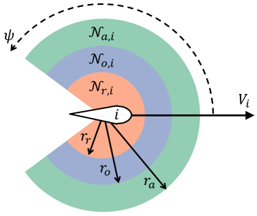
Figure 1: An individual is assumed to be able to evaluate the relative positions of other individuals within the sensing region that has radius $r_{a}$ and cone angle $2\psi$. The sensing region is divided into the region of repulsion, orientation, and attraction.

Finally, we describe the definitions of the regions of repulsion, orientation, and attraction used in [19]. We first introduce a constant $\psi>0$, which represents the viewing angle of the fishes. Then, we define the cone $C_{i}(k)=\{z\in\mathbb{R}^{3}\mid\angle(V_{i}(k),z-x_{i}(k))\leq\psi\}$. Under this notation, the authors in [19] adopt the definition (see Fig. 1 for an illustration)

$$Z_{r,i}(k) =C_{i}(k)\cap\{z\in\mathbb{R}^{3}\mid 0<\lVert z-x_{i}(k)\rVert\leq r_{r}\},$$

$$Z_{o,i}(k) =C_{i}(k)\cap\{z\in\mathbb{R}^{3}\mid r_{r}<\lVert z-x_{i}(k)\rVert\leq r_{o}\},$$

$$Z_{a,i}(k) =C_{i}(k)\cap\{z\in\mathbb{R}^{3}\mid r_{o}<\lVert z-x_{i}(k)\rVert\leq r_{a}\},$$

where the positive constants $r_{r}$, $r_{o}$, and $r_{a}$ are called the radius of repulsion, orientation, and attraction, respectively, and they are supposed to satisfy $0<r_{r}<r_{o}<r_{a}$. The angle $\psi$ is assumed to be strictly less than $\pi$ to model a blind zone in the visual field of fish.

The current model extends the well-known Boid model [47] by focusing on fish schooling. Further, the current model extends a previous model [16] for swarming behaviors by improving the treatment of noise. In the current model, a noise is designed to always affect the direction of fish, which is not the case in the model presented in [16].

3.2 Controlled Model

The fish schooling model proposed by Gautrais et al. [19] does not consider the possibility of external stimulus to the fish school. In this paper, we adopt a simple modification of the model to incorporate external stimulus. For simplicity, we assume that the stimulus attracts the $i$th fish to the direction of a unit vector $u_{i}\in\mathbb{R}^{3}$. Further, we assume that each fish has its own sensitivity parameter $\xi_{i}\geq 0$, which can account for the heterogeneity within the swarm of fishes. We then propose that the original equation (6) for the desired direction be modified as

$$D_{i}(k)=\begin{cases}O_{i}(k)+\eta A_{i}(k)+\xi_{i}u_{i}(k),&\mbox{if $\mathcal{N}_{r,i}(k)=\emptyset$,}\\ {E}_{i}(k),&\mbox{otherwise.}\end{cases}$$ (8)

We introduce the notation $u_{i}$ for the generality of the theory developed in this paper; although the notation $u_{i}$ suggests the possibility of applying stimulus $u_{i}$ designed independently for each individual, realizing such a stimulus is not realistic. In reality, the degree of freedom in designing the set of stimulus $\{u_{i}\}_{i=1}^{N}$ can be severely limited.

3.3 Tracking Problem

We consider a tracking problem for the controlled schooling model introduced in the last subsection. Assume that a reference set $\mathcal{R}\subset\mathbb{R}^{3}$ is given. Our objective is to design the external stimulus $u_{i}$ ($i=1,\dotsc,N$) appearing in (8) to guide the fish school and make the mass center

$$c=\frac{1}{N}\sum_{i=1}^{N}x_{i}$$ (9)

of the fish school lie on the set $\mathcal{R}$. The closeness is measured by the distance

$$e(k)=\operatorname{dist}(c(k),\mathcal{R}),$$ (10)

where $\operatorname{dist}(\cdot,\cdot)$ denotes the distance between a vector and a subset of $\mathbb{R}^{3}$ and is defined by $\operatorname{dist}(y,\mathcal{Z})=\inf\{\lVert y-z\rVert\mid z\in\mathcal{Z}\}$.

The following control problem is considered in this paper. We assume that, at every $T$ discrete steps (i.e., at every $T\tau$ units of time in the continuous time), we can observe the fish school to obtain positions and directions of all fish. Further, we assume that we can update the value of the external stimulus $u_{i}$ only at the time of these observations; i.e., for all $i\in\{1,\dotsc,N\}$ and $\ell\geq 0$, we impose the constraint

$$u_{i}(\ell T)=u_{i}(\ell T+1)=\cdots=u_{i}((\ell+1)T-1).$$ (11)

We use the observation $\{x_{i}(\ell T),V_{i}(\ell T)\}_{i=1,\dotsc,N}$ at the $\ell$th step for determining the stimulus within the subsequent sampling interval (i.e., at times $k=(\ell+1)T,(\ell+1)T+1,\dotsc,(\ell+2)T-1$). Therefore, it is required that the stimulus computation finishes within $T\tau$ units of time in the continuous time.

The high nonlinearity of the schooling model suggests that the framework of the MPC is appropriate to determine the stimulus. Therefore, let us consider the scenario where we determine the stimulus by iteratively solving finite-horizon optimization problems to minimize the cost function

$$\sum_{k=(\ell+1)T}^{(\ell+1)T+T_{h}}{e(k)},$$

where $T_{h}>0$ denotes the length of the optimization horizon.

One obvious option for prediction is to use the original schooling model. In this prediction model, one can use the original schooling dynamics as is except with the rotation dynamics (7) replaced by

$$V_{i}(k+1)=R_{D_{i}(k){,\phi_{i}(k)}}V_{i}(k),$$ (12)

where the random rotation operator $R_{\chi_{i}(k){,\epsilon_{i}(k)}}$ is set to the identity operator. This prediction model, denoted by $\Sigma_{\operatorname{orig}}$, results in the following optimization problem to be solved during the continuous-time interval $[\ell T\tau,(\ell+1)T\tau)$:

$$\operatorname*{\ \ \ minimize\ \ \ }_{\{u(k)\}_{k=(\ell+1)T}^{(\ell+1)T+T_{h}-1}} \sum_{k=(\ell+1)T}^{(\ell+1)T+T_{h}}{e(k)}$$ (13)

$$\operatorname*{\ \ \ subject\ to\ \ \ }$$ 1, 2, 3, 4, 8, 11, 12, 9 and 10

for determining the control input $\{u(k)\}_{k=(\ell+1)T}^{k=(\ell+2)T-1}$ to be used in the next (continuous-time) interval $[(\ell+1)T\tau,(\ell+2)T\tau)$. A schematic of the control algorithm is illustrated in Fig. 2. Although the optimization problem (13) based on $\Sigma_{\operatorname{orig}}$ could allow us to realize precise tracking by the fish school, a natural concern in this context is the computational cost for performing predictions, because the number of inter-fish interactions in the model grows quadratically with respect to the size $N$ of the school. This potential numerical difficulty is illustrated in Section 5. Thus, it is desirable to construct reduced-order prediction models for performing numerically efficient MPC.

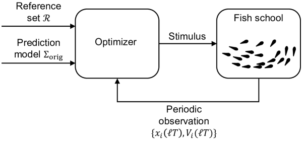
Figure 2: Schematic of MPC with the original schooling model $\Sigma_{\operatorname{orig}}$. The positions and directions of each individual are measured periodically. Using the measurement, reference set $\mathcal{R}$, and model $\Sigma_{\operatorname{orig}}$, the optimizer periodically updates the stimulus applied to individuals.

4 Reduced-order MPC

We present reduced-order models for the fish schooling model based on static weights and centrality-based weights, respectively. Based on the reductions, we then present reduced-order MPC algorithms for solving the tracking problem introduced in the last section. Throughout this section, we use the following notation. For a set of vectors $v_{1},\dotsc,v_{N}$ with the same dimension and scalars $\alpha_{1},\dotsc,\alpha_{N}$, we write

$$\langle v\rangle_{\alpha}=\sum_{i=1}^{N}\alpha_{i}v_{i}.$$

In the special case where $\alpha_{1}=\cdots=\alpha_{N}=p$ for a constant $p$, we write

$$\langle v\rangle_{p}=p\sum_{i=1}^{N}v_{i}.$$ (14)

4.1 Static Weight

We propose a static weight-reduction of the model $\Sigma_{\operatorname{orig}}$ for predicting the trajectory of the mass center $c(k)$. We begin by outlining our overall idea. Under notation (14), we have

$$c(k+1)=c(k)+\tau v\langle V(k)\rangle_{1/N}.$$ (15)

Therefore, if we could construct an update low for $\langle V\rangle_{1/N}$ in terms of $c$ and $\langle V\rangle_{1/N}$, then the update law in conjunction with (15) serves as a reduced-order model for predicting the movement of the mass center. To proceed, let us tentatively consider the scenario in which the rotation speed $\theta$ is relatively high. In this situation, one can expect that the fish in the school can easily rotate to align with their desired directions. Indeed, for a sufficiently large $\theta$, equation (12) implies $V_{i}(k+1)=\phi(D_{i}(k))$, which further implies

$$\langle V(k+1)\rangle_{1/N}=\langle\phi(D(k))\rangle_{1/N}.$$

Therefore, approximation of $\langle\phi(D(k))\rangle_{1/N}$ in terms of $c$ and $\langle V\rangle_{1/N}$ allows us to construct a reduced-order model for prediction of the mass center.

Motivated by this observation, we propose an approximation formula for computing the quantity $\langle\phi(D(k))\rangle_{1/N}$. For the sake of generality of the theoretical development, we allow the weight $1/N$ to be arbitrary nonnegative numbers $\alpha_{1}$, …, $\alpha_{N}$ satisfying

$$\sum_{i=1}^{N}\alpha_{i}=1.$$ (16)

4.1.1 Reduction Error Analysis

We present some notations. Let $i,j\in\{1,\dotsc,N\}$ and $k\geq 0$ be arbitrary. For the $i$th fish, let

$$n_{i}(k)=\lvert\mathcal{N}_{o,i}(k)\rvert$$

denote the number of its neighbors within the region of orientation. Define $\omega_{ij}(k)\in\{0,1\}$ by

$$\omega_{ij}(k)=\begin{cases}1,&\mbox{if $j\in\mathcal{N}_{o,i}(k)$},\\ 0,&\mbox{otherwise.}\end{cases}$$

In addition, let $\theta_{ij}(k)=\angle(V_{i}(k),V_{j}(k))$ denote the angle between the directions of the $i$th and $j$th fish. Then, for a vector $y=[y_{1},\,\dotsc,y_{N}]^{\top}\in\mathbb{R}^{N}$, we define a quadratic function of the angles as

$$\begin{multlined}Q_{i,y}(k)=\frac{1}{n_{i}(k)^{2}}\sum_{j=1}^{N}\sum_{j^{\prime}=1}^{N}\frac{\lvert\omega_{ij}(k)-y_{j}\rvert\lvert\omega_{ij^{\prime}}(k)-y_{j}^{\prime}\rvert}{2}\theta_{jj^{\prime}}(k)^{2}.\end{multlined}Q_{i,y}(k)=\frac{1}{n_{i}(k)^{2}}\sum_{j=1}^{N}\sum_{j^{\prime}=1}^{N}\frac{\lvert\omega_{ij}(k)-y_{j}\rvert\lvert\omega_{ij^{\prime}}(k)-y_{j}^{\prime}\rvert}{2}\theta_{jj^{\prime}}(k)^{2}.$$

Further, we introduce constants that play an important role in our analysis. First, define

$$\tilde{\pi}_{i}(k)=1-\pi_{i}(k)\in[0,1],$$

where $\pi_{i}(k)=\lVert O_{i}(k)\rVert/n_{i}(k)\in[0,1]$ represents the polarization [48, 16, 19] of the fish in the region of orientation $Z_{o,i}(k)$. We use the constant $\tilde{\pi}_{i}(k)$ to quantify how aligned the directions of the fish in the region of orientation $Z_{o,i}(k)$ are; the smaller $\tilde{\pi}_{i}(k)$, the more aligned are the directions of the fish in the region. Similarly, we define

$$\tilde{\pi}_{\alpha}(k)=1-\lVert\langle V(k)\rangle_{\alpha}\rVert\in[0,1],$$

which quantifies how aligned the directions of all the fish are when weighted with $\alpha$. We define the ratio

$$\rho_{i}(k)=\frac{\lVert\eta A_{i}(k)+\xi_{i}u_{i}(k)\rVert}{\lVert O_{i}(k)\rVert}\geq 0.$$

This quantity measures how dominant the force of orientation is in the desired direction (8) when repulsion is absent. For example, if $\rho_{i}(k)=0$, both $A_{i}(k)$ and $u_{i}(k)$ are zero, and therefore, the movement of the $i$th fish is completely determined by the orientation term $O_{i}(k)$.

Our objective is to propose an approximation formula for $\langle\phi(D(k))\rangle_{\alpha}$ weighted by $\alpha$. Let us consider the approximation

$$\langle\phi(D(k))\rangle_{\alpha}\approx\lVert\langle V(k)\rangle_{\alpha}\rVert\,\phi\bigl{(}\langle V(k)\rangle_{\alpha}+A(k)+u(k)\bigr{)}$$ (17)

with vectors

$$A(k)=\sum_{i=1}^{N}\frac{\alpha_{i}}{n_{i}(k)}\eta A_{i}(k),\ u(k)=\sum_{i=1}^{N}\frac{\alpha_{i}}{n_{i}(k)}\xi_{i}u_{i}(k)$$ (18)

which represent the aggregated force of attraction and external stimulus, respectively. Now, the following theorem provides a bound for the approximation (17). Within the theorem, the dependence of relevant variables on the time index $k$ is omitted for brevity.

Theorem 4.1.

Assume that

$$\mathcal{N}_{r,i}=\emptyset$$ (19)

and

$${n_{i}>0,}\quad O_{i}\neq 0$$ (20)

for all $i=1,\dotsc,N$. Let $\alpha_{1}$, …, $\alpha_{N}$ be nonnegative constants satisfying (16). If $\langle V\rangle_{\alpha}\neq 0$, then the norm of the residual vector

$$\epsilon_{\alpha}=\langle\phi(D)\rangle_{\alpha}-\lVert\langle V\rangle_{\alpha}\rVert\,\phi\bigl{(}\langle V\rangle_{\alpha}+A+u\bigr{)}$$ (21)

satisfies

$$\begin{multlined}\lVert\epsilon_{\alpha}\rVert\leq 2\frac{\lVert A+u\rVert^{2}}{\lVert\langle V\rangle_{\alpha}\rVert}+\sum_{i=1}^{N}\alpha_{i}\left(\tilde{\pi}_{i}+\sqrt{Q_{i,n_{i}\alpha}}\right)\\ +2\sum_{i=1}^{N}\alpha_{i}\rho_{i}\left(\tilde{\pi}_{\alpha}+\rho_{i}+2\tilde{\pi}_{i}+\sqrt{Q_{i,n_{i}\alpha}}\right).\end{multlined}\lVert\epsilon_{\alpha}\rVert\leq 2\frac{\lVert A+u\rVert^{2}}{\lVert\langle V\rangle_{\alpha}\rVert}+\sum_{i=1}^{N}\alpha_{i}\left(\tilde{\pi}_{i}+\sqrt{Q_{i,n_{i}\alpha}}\right)\\ +2\sum_{i=1}^{N}\alpha_{i}\rho_{i}\left(\tilde{\pi}_{\alpha}+\rho_{i}+2\tilde{\pi}_{i}+\sqrt{Q_{i,n_{i}\alpha}}\right).$$ (22)

Proof.

See A. ∎

Remark 4.2.

Condition (19) in Theorem 4.1 is motivated and supported by our empirical finding that the repulsion term $R_{i}(k)$ defined in (2) does not become active frequently. Similarly, the second condition (20) is not very restrictive when a given group of fish form one school.

Before presenting the proof of the theorem, we briefly provide an interpretation of the bound. The bound suggests the following two scenarios in which the approximation (17) is precise:

• The force of attraction $\eta A_{i}$ and the stimulus $\xi_{i}u_{i}$ are small

• The direction of individuals are aligned

Specifically, the following corollary illustrates which terms in the bound are critical in these two situations.

Corollary 4.3.

Let $\alpha_{1}$, …, $\alpha_{N}$ be nonnegative constants satisfying (16). Assume that inequalities (19) and (20) hold. If $A_{i}=u_{i}=0$ for all $i\in\{1,\dotsc,N\}$, then

$$\lVert\epsilon_{\alpha}\rVert\leq\sum_{i=1}^{N}\alpha_{i}\left(\tilde{\pi}_{i}+\sqrt{Q_{i,n_{i}\alpha}}\right).$$ (23)

On the other hand, if $\theta_{ij}=0$ for all $i,j\in\{1,\dotsc,N\}$, then

$$\lVert\epsilon_{\alpha}\rVert\leq 2\left(\lVert A+u\rVert^{2}+\sum_{i=1}^{N}\alpha_{i}\lVert\eta A_{i}+\xi_{i}u_{i}\rVert^{2}\right).$$ (24)

4.1.2 Prediction Model

Our discussion at the beginning of this section and Theorem 4.1 suggest the approximation

$$\langle V(k+1)\rangle_{{1/N}}\approx\lVert\langle V(k)\rangle_{{1/N}}\rVert\,\phi\bigl{(}\langle V(k)\rangle_{{1/N}}+A(k)+u(k)\bigr{)}.$$ (25)

This approximation motivates us to construct the following lower-order prediction model, which we denote by $\Sigma_{\operatorname{stc}}$. In this model, at an observation time $k=\ell T$, the estimated center of mass $\hat{c}$ is initialized as

$$\hat{c}(\ell T)=\frac{1}{N}\sum_{i=1}^{N}x_{i}(\ell T),$$ (26)

and it is dynamically updated by the difference equation

$$\hat{c}(k+1)=\hat{c}(k)+\tau v\hat{V}(k),$$ (27)

where $\hat{V}$ represents the estimated direction of the center of mass and is dynamically updated as in (25) by

$$\begin{multlined}\hat{V}(k+1)=\lVert\hat{V}(k)\rVert\,\phi\bigg{(}\hat{V}(k)+\sum_{i=1}^{N}\frac{{1/N}}{n_{i}(\ell T)}\eta A_{i}(\ell T)+\sum_{i=1}^{N}\frac{{1/N}}{n_{i}(\ell T)}\xi_{i}u_{i}(k)\bigg{)}\end{multlined}\hat{V}(k+1)=\lVert\hat{V}(k)\rVert\,\phi\bigg{(}\hat{V}(k)+\sum_{i=1}^{N}\frac{{1/N}}{n_{i}(\ell T)}\eta A_{i}(\ell T)+\sum_{i=1}^{N}\frac{{1/N}}{n_{i}(\ell T)}\xi_{i}u_{i}(k)\bigg{)}$$ (28)

for $k\geq\ell T$ under the initialization

$$\hat{V}(\ell T)=\frac{1}{N}\sum_{i=1}^{N}V_{i}(\ell T)$$ (29)

at time $k=\ell T$. Therefore, the optimization problem to be solved during the continuous-time interval $[\ell T\tau,(\ell+1)T\tau)$ to determine the stimulus to be used in the next interval $[(\ell+1)T\tau,(\ell+2)T\tau)$ is

$$\operatorname*{\ \ \ minimize\ \ \ }_{\{u(k)\}_{k=(\ell+1)T}^{(\ell+1)T+T_{h}-1}} \sum_{k=(\ell+1)T}^{(\ell+1)T+T_{h}}\operatorname{dist}(\hat{c}(k),\mathcal{R})$$ (30)

$$\operatorname*{\ \ \ subject\ to\ \ \ }$$ 26, 27, 28 and 29.

A schematic of the control algorithm is illustrated in Fig. 3. The quantities required to solve this optimization problem are the observations $\{x_{i}(\ell T),V_{i}(\ell T)\}_{i=1}^{N}$ and the parameters $\psi$, $\eta$, $\xi_{i}$, $N$, $\tau$, $v$, $r_{r}$, $r_{o}$, and $r_{a}$. If the exact values of the parameters are not available, they can be replaced with estimates.

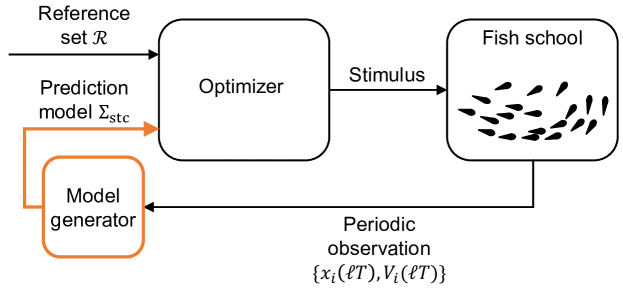
Figure 3: A schematic of MPC with the reduced-order model $\Sigma_{\operatorname{stc}}$. The positions and directions of each individual are measured periodically. Using the measurement, we construct reduced-order model $\Sigma_{\operatorname{stc}}$ for prediction. Using the model in place of $\Sigma_{\operatorname{orig}}$, the optimizer periodically updates the stimulus applied to individuals.

4.2 Dynamic Weight

We closely analyzed the error from a dimension reduction of the controlled fish school model and introduced a reduced-order prediction model for the schooling. In the reduction, the weights for aggregating the directions of the fish in the school were assumed to be constant. Then, the natural question is to ask whether allowing the weights to change dynamically over time dependent on the state of the school would lead to a more precise reduction of the model.

To provide an affirmative answer to the aforementioned question, in this section, we present a dynamic weight-reduction of the controlled fish schooling model and, then, present yet another model for predicting the mass center of the fish school. We show that the reduction weighted by the normalized eigenvector centrality of the interaction network induced by forces of orientation allows us to improve the error bound (22) for static weights.

Let us recall the definition of the normalized eigenvector centrality of directed networks. Let $\mathcal{G}=(V,E)$ be a directed and unweighted graph having nodes $V=\{1,\dotsc,N\}$. We denote an directed edge from node $i$ to node $j$ by $(i,j)$. For each $i\in V$, let $d_{\operatorname{out}}(i)$ denote the outdegree of node $i$. The normalized adjacency matrix of $\mathcal{G}$ is the $N\times N$ matrix defined by

$$W_{ij}=\begin{cases}{1}/{d_{\operatorname{out}}(i)},&\mbox{if $(i,j)\in E$,}\\ 0,&\mbox{otherwise.}\end{cases}$$

If $\mathcal{G}$ is strongly connected, the normalized eigenvector centrality of $\mathcal{G}$ is defined as the positive vector $\beta=[\beta_{1}\ \cdots\ \beta_{N}]^{\top}$ satisfying $W^{\top}\beta=\beta$ and $\beta_{1}+\cdots+\beta_{N}=1$.

4.2.1 Reduction Error Analysis

We first provide a brief discussion to demonstrate the need for using the normalized eigenvector centrality of the interaction network induced by forces of orientation. We consider the scenario where the orientation force $O_{i}(k)$ is a dominant term in the desired direction $D_{i}(k)$. In this scenario, we can invoke the rough approximation $\lVert D_{i}(k)\rVert\approx n_{i}(k)$, which leads to

$${D_{i}(k)\approx\frac{1}{n_{i}}(O_{i}+\eta A_{i}+\xi_{i}w_{i}).}$$ (31)

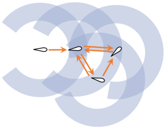
Figure 4: Interaction network $\mathcal{G}_{o}$ of a fish school with $N=4$ individuals. Blue areas represent the regions of orientation of each individuals.

Now, we define the interaction network $\mathcal{G}_{o}(k)$ induced by forces of orientation as the directed and unweighted network in which nodes are fish in the school and edge $(i,j)$ exists if and only if $j\in\mathcal{N}_{o,i}(k)$ (Fig. 4). Let $W_{o}(k)$ denote the normalized adjacency matrix of the network $\mathcal{G}_{o}(k)$. Then, a straightforward calculation shows

$$\sum_{i=1}^{N}\alpha_{i}\frac{1}{n_{i}(k)}O_{i}(k) =\sum_{i=1}^{N}\alpha_{i}\frac{1}{n_{i}(k)}\sum_{j=1}^{N}\omega_{ij}(k)V_{j}(k)$$ (32)

$$=\langle V(k)\rangle_{W_{o}(k)^{\top}\alpha}.$$

Therefore, from (31), we obtain

$$\langle D(k)\rangle_{\alpha}\approx\langle V(k)\rangle_{W_{o}(k)^{\top}\alpha}+A(k)+u(k),$$

where $A(k)$ and $u(k)$ are defined in (18). This approximate relationship contains a potential inconsistency in the weights on the desired direction $D$ and the direction $V$. The inconsistency can be resolved if weight $\alpha$ satisfies $\alpha=W_{o}(k)^{\top}\alpha$, i.e., if $\alpha$ equals the normalized eigenvector centrality of network $\mathcal{G}_{o}(k)$. This discussion suggests that the aggregation of direction $V$ by the normalized eigenvector centrality can allow us to construct a reduced-order model with a higher accuracy.

The following theorem provides a theoretical confirmation on the potential superiority of model reduction with the normalized eigenvector centrality over the one with a static weight. The dependence of relevant variables on the time index $k$ is omitted for brevity, as in Theorem 4.1.

Theorem 4.4.

Assume that (19) and (20) hold true for all $i=1,\dotsc,N$. Suppose that $\alpha$ equals the normalized eigenvector centrality of $\mathcal{G}_{o}$. If $\langle V\rangle_{\alpha}\neq 0$, then the vector $\epsilon_{\alpha}$ defined in (21) satisfies

$$\begin{multlined}\lVert\epsilon_{\alpha}\rVert\leq 2\frac{\lVert A+u\rVert^{2}}{\lVert\langle V\rangle_{\alpha}\rVert}+\sum_{i=1}^{N}\alpha_{i}\tilde{\pi}_{i}+2\sum_{i=1}^{N}\alpha_{i}\rho_{i}\left(\tilde{\pi}_{\alpha}+\rho_{i}+2\tilde{\pi}_{i}+\sqrt{Q_{i,n_{i}\alpha}}\right).\end{multlined}\lVert\epsilon_{\alpha}\rVert\leq 2\frac{\lVert A+u\rVert^{2}}{\lVert\langle V\rangle_{\alpha}\rVert}+\sum_{i=1}^{N}\alpha_{i}\tilde{\pi}_{i}+2\sum_{i=1}^{N}\alpha_{i}\rho_{i}\left(\tilde{\pi}_{\alpha}+\rho_{i}+2\tilde{\pi}_{i}+\sqrt{Q_{i,n_{i}\alpha}}\right).$$ (33)

Proof.

See Appendix B. ∎

The bound of the reduction error in (33) does not have the term $\sum_{i=1}^{N}\alpha_{i}\sqrt{Q_{i,n_{i}\alpha}}$, which is a major term in estimates (22) and (23) from using static weights. This fact suggests that using the normalized eigenvector centrality as the weight for reduction can lead to a more precise prediction of fish schooling.

The following corollary is the dynamic-weight counterpart of Corollary 4.3 and explicitly shows the improvement of estimate (23).

Corollary 4.5.

Assume that (19) and (20) hold true for all $i=1,\dotsc,N$. Suppose that $\alpha$ equals the normalized eigenvector centrality of $\mathcal{G}_{o}$. If $A_{i}=u_{i}=0$ for all $i\in\{1,\dotsc,N\}$, then

$$\lVert\epsilon_{\alpha}\rVert\leq\sum_{i=1}^{N}\alpha_{i}\tilde{\pi}_{i}.$$

On the other hand, if $\theta_{ij}=0$ for all $i,j\in\{1,\dotsc,N\}$, then inequality (24) holds.

4.2.2 Prediction Model

We present our second reduced-order model $\Sigma_{\operatorname{dyn}}$ based on Theorem 4.4. In this model, although the estimated center of mass $\hat{c}$ is initialized and updated by equations (26) and (27) as in the first model $\hat{\Sigma}_{\operatorname{stc}}$, the update law for the estimated direction $\hat{V}$ is distinct and given by

$$\begin{multlined}\hat{V}(k+1)=\lVert\hat{V}(k)\rVert\,\phi\bigg{(}\hat{V}(k)+\sum_{i=1}^{N}\frac{\beta_{i}(\ell T)}{n_{i}(\ell T)}\eta A_{i}(\ell T)+\sum_{i=1}^{N}\frac{\beta_{i}(\ell T)}{n_{i}(\ell T)}\xi_{i}u_{i}(k)\bigg{)}\end{multlined}\hat{V}(k+1)=\lVert\hat{V}(k)\rVert\,\phi\bigg{(}\hat{V}(k)+\sum_{i=1}^{N}\frac{\beta_{i}(\ell T)}{n_{i}(\ell T)}\eta A_{i}(\ell T)+\sum_{i=1}^{N}\frac{\beta_{i}(\ell T)}{n_{i}(\ell T)}\xi_{i}u_{i}(k)\bigg{)}$$ (34)

for $k=\ell T,\ell T+1,\dotsc$, where $\beta_{1}(\ell T)$, …, $\beta_{N}(\ell T)$ denote the normalized eigenvector centrality of the network $\mathcal{G}_{o}(\ell T)$. In this construction, we implicitly utilize the approximation $\langle V\rangle_{\alpha}\approx\langle V\rangle_{1/N}$. Therefore, we use the same initialization (29) of $\hat{V}$ as in $\Sigma_{\operatorname{stc}}$. Hence, the optimization problem to be solved during the continuous-time interval $[\ell T\tau,(\ell+1)T\tau)$ for determining the stimulus to be used in the next interval $[(\ell+1)T\tau,(\ell+2)T\tau)$ is

$$\operatorname*{\ \ \ minimize\ \ \ }_{\{u(k)\}_{k=(\ell+1)T}^{(\ell+1)T+T_{h}-1}} \sum_{k=(\ell+1)T}^{(\ell+1)T+T_{h}}\operatorname{dist}(\hat{c}(k),\mathcal{R})$$ (35)

$$\operatorname*{\ \ \ subject\ to\ \ \ } \lx@cref{creftypeplural~refnum}{eq:hatxinitialize},\lx@cref{refnum}{eq:hatxupdate},\lx@cref{refnum}{eq:isreferred_hatvupdateddyn}and~\lx@cref{refnum}{eq:initialCond}.$$

Although the prediction model $\Sigma_{\operatorname{dyn}}$ is more elaborated than $\Sigma_{\operatorname{stc}}$, the set of quantities we require to solve this optimization problem is the same as the one for the optimization problem (30).

Theorem 4.4 suggests the possibility that model $\Sigma_{\operatorname{dyn}}$ achieves smaller prediction errors compared with the static weight-based model $\Sigma_{\operatorname{stc}}$ because we can expect that the MPC with the model $\Sigma_{\operatorname{dyn}}$ can be better than the one with $\Sigma_{\operatorname{stc}}$. We confirm the superiority of the prediction model $\Sigma_{\operatorname{dyn}}$ in the next section.

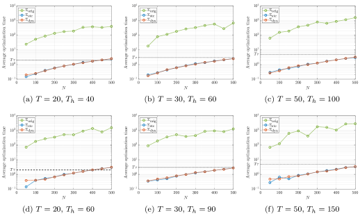
Figure 5: Average of optimization times in one instance of MPC with prediction models $\Sigma_{\operatorname{orig}}$, $\Sigma_{\operatorname{stc}}$, and $\Sigma_{\operatorname{dyn}}$. The reference set has radius $r_{{\operatorname{ref}}}=2000$. The optimization with the raw prediction model $\Sigma_{\operatorname{orig}}$ does not complete within the required $T\tau$ seconds in any of the cases, whereas the MPC with the reduced-order prediction models is both successful for fish schools with up to $N=350$ individuals for any pair $(T,T_{h})$.

5 Numerical Simulation

In this section, we present numerical simulations and illustrate the effectiveness of the MPC with the reduced-order prediction models. Further, we numerically show that the dynamic-weight prediction model allows us to perform better tracking than that with the static-weight prediction model. Simulations have been performed with MATLAB 2021a on a desktop computer with Xeon Gold 5218R processors and 96 GB DRAMs. We used the nonlinear programming solver of fmincon to solve the optimization problems (13), (30), and (35).

In this numerical simulation, we assume that the fish school consists of homogeneous individuals with the same sensitivity; i.e., we suppose the existence of a positive constant $\xi$ such that $\xi_{1}=\cdots=\xi_{N}=\xi$. We further assume, for the purpose of simplicity and illustration, that the same control input is uniformly applied to all individuals in the school. Therefore, we assume $u_{1}(k)=\cdots=u_{N}(k)$ for all $k$. We follow the reference [19] and set the relevant parameters of the fish school as $v=50$, $\psi={3\pi/4}$, $\theta=0.69$ [rad], $\eta=1$, $r_{r}=50$, $r_{o}=750$, and $r_{a}=$1000$$. We set the noise level to be 10 times of the one suggested by the authors in [19] to make the tracking harder. We set the sampling interval for discretization to be $\tau=0.1$; the common sensitivity parameter is set as $\xi=10$.

We suppose that reference set $\mathcal{R}$ is the surface of a sphere centered at the origin with radius $r_{{\operatorname{ref}}}$. To determine the initial positions of fish in the school, we first place each fish by drawing from the uniform distribution in a sphere with radius $r_{a}/2$. Then, the entire set of fish is uniformly shifted so that the mass center $c(0)$ of the school is located on a point on the reference set $\mathcal{R}$. Our choice of the radius $r_{a}/2$ guarantees that the initial fish school is sufficiently large so that both orientation (3) and the attraction (4) forces are in effect, while ensuring that each pair of fish is within the interaction distance to avoid the fragmentation of the school.

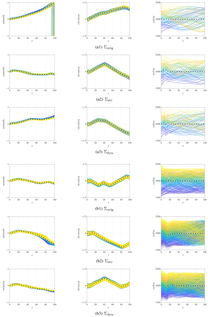
Figure 6: Azimuth (left), elevation (middle), and radius (right) of positions $x_{i}(k)$ of individual fish (solid lines) controlled with prediction models $\Sigma_{\operatorname{orig}}$, $\Sigma_{\operatorname{stc}}$, and $\Sigma_{\operatorname{dyn}}$. Dashed line represent the mass center $c(k)$ of fish school. The reference set has radius $r_{{\operatorname{ref}}}=2000$. a1-a3: $N=100$. b1-b3: $N=300$.

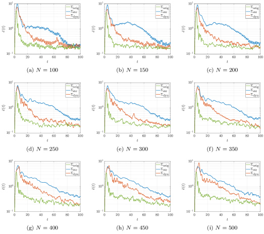
Figure 7: Average tracking errors in the MPC with prediction models $\Sigma_{\operatorname{orig}}$ (green), $\Sigma_{\operatorname{stc}}$ (blue), and $\Sigma_{\operatorname{dyn}}$ (red). The reference set has radius $r_{{\operatorname{ref}}}=2000$. Overall, the MPC with the prediction model $\Sigma_{\operatorname{dyn}}$ performs better than the one with model $\Sigma_{\operatorname{stc}}$ using static weights. Furthermore, the MPC with the prediction model $\Sigma_{\operatorname{dyn}}$ performs asymptotically as good as the one with the original prediction model $\Sigma_{\operatorname{orig}}$.

5.1 Computation Time

We investigate the amount of reduction in computation time required to perform the MPC. Let the radius of the reference sphere be $r_{{\operatorname{ref}}}=2r_{a}=$2000$$. We examine the following three different scenarios on period $T$ of observation and actuation: $T=20$, $30$, and $50$. For each $T$, we consider two different lengths of the optimization horizon $T_{h}$: $T_{h}=2T$ and $T_{h}=3T$. For all six cases, we perform the following simulation. We randomly set the initial positions and directions of schools of fish with $N=50$, $100$, $150$, …, $500$ individuals. We then perform one instance of MPC using the three prediction models $\Sigma_{\operatorname{orig}}$, $\Sigma_{\operatorname{stc}}$, and $\Sigma_{\operatorname{dyn}}$ on the discrete-time interval $\{0,1,\dotsc,1000\}$ (i.e., the continuous-time interval $[0,100]$). Then, we measure the average of the computation time of finite-horizon optimizations.

In Fig. 5, we present the average of the computation time of finite-horizon optimizations with each of the prediction models (i.e., the optimization problems in (13), (30), and (35)) and for the six pairs $(T,T_{h})$. Optimization with the raw prediction model $\Sigma_{\operatorname{orig}}$ does not complete within the required $T\tau$ seconds in any case. The MPC with the reduced-order prediction models is both successful for fish schools with up to $N=350$ individuals for any case, which confirms the computational effectiveness of model reduction.

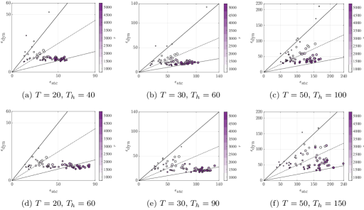
Figure 8: Asymptotic cumulative tracking errors $\epsilon_{\operatorname{stc}}$ and $\epsilon_{\operatorname{dyn}}$ from MPC with static and dynamic weight-prediction models, respectively. Each circle represents data from performing 100 control trials for a fixed pair $(N,r_{{\operatorname{ref}}})$. Area of each circle is proportional to $N$. Colors of markers represent $r_{{\operatorname{ref}}}$. Solid, dashed, and dotted lines represent the straight lines $\epsilon_{\operatorname{dyn}}=\epsilon_{\operatorname{stc}}$, $\epsilon_{\operatorname{dyn}}=\epsilon_{\operatorname{stc}}/2$, and $\epsilon_{\operatorname{dyn}}=\epsilon_{\operatorname{stc}}/5$, respectively. Overall, the errors from the dynamic weight-model is smaller than the ones from the static weight-model for most of the cases.

5.2 Tracking Performance

We compare the tracking performances. To this end, we fix $r_{{\operatorname{ref}}}=2000$ and perform the MPC of the fish school consisting of $N=100$ and $300$ individuals. The simulation results are illustrated in Fig. 6. We show the azimuth, elevation, and radius of the position of all individuals and the mass center. For both school sizes, we confirm that the MPC with all prediction models realize stable tracking to the sphere.

We vary the school sizes and observe the average tracking errors to further compare the tracking performance of the MPC with the three prediction models. We perform 100 instances of MPC over the same time interval with different initial positions and directions for each school size $N$. Then, we calculate the empirical average $\bar{e}$ of the tracking error $e$ defined in (10). The obtained empirical averages of the tracking errors are presented in Fig. 7. We observe an overall trend in which the MPC with $\Sigma_{\operatorname{dyn}}$ performs better than the one with $\Sigma_{\operatorname{stc}}$ using static weights. We also find that the MPC with $\Sigma_{\operatorname{dyn}}$ performs asymptotically as good as the one with $\Sigma_{\operatorname{orig}}$. These trends suggest the effectiveness of dynamically changing the weights on model reduction, which confirms our theoretical findings on the reduction errors in Theorems 4.1 and 4.4.

Let us perform a more thorough comparison of the MPC with $\Sigma_{\operatorname{dyn}}$ and $\Sigma_{\operatorname{stc}}$. We focus on these two models because the MPC with $\Sigma_{\operatorname{orig}}$ does not complete within the required time as observed in Fig. 5. We specifically compare the average of the asymptotic and cumulative tracking error

$$\epsilon=\int_{50}^{100}\bar{e}(t)\,dt$$

for various pairs $(N,r_{{\operatorname{ref}}})$ of the parameters. In this simulation, we vary $N$ within the set $\{50,100,\dotsc,500\}$, while we vary the radius $r_{{\operatorname{ref}}}$ of the reference sphere $\mathcal{R}$ within the set $\{1000,1500,\dotsc,5000\}$. For each pair $(N,r_{{\operatorname{ref}}})$, we run 100 instances of MPC on the discrete-time interval $\{0,1,2,\dotsc,1000\}$ using each prediction model. We plot errors $\epsilon_{\operatorname{dyn}}$ and $\epsilon_{\operatorname{stc}}$ from the dynamic and static prediction models, respectively, in Fig. 8. The errors from the dynamic weight-model are smaller than those from the static weight-model for most cases, which confirms the effectiveness of using the dynamic weight-model for prediction. We also remark that, while $\epsilon_{\operatorname{dyn}}$ is not heavily dependent on the optimization horizon $T_{h}$, $\epsilon_{\operatorname{stc}}$ becomes larger for the longer optimization horizon $T_{h}=3T$. This phenomena can be attributed to the relative inaccuracy of the static prediction model $\Sigma_{\operatorname{stc}}$. Further, we observe the trend that the larger the radius $r_{\operatorname{ref}}$ of the reference set $\mathcal{R}$, the smaller is the relative accuracy $\epsilon_{\operatorname{dyn}}/\epsilon_{\operatorname{stc}}$ of the MPC with dynamic weights. From this trend, we can infer that the MPC with the dynamic weights exhibit its superiority for tracking a reference set with a small curvature. Further, for small schools, the MPC with dynamic weights does not necessarily outperform the one with static weights.

Therefore, we have confirmed the superiority of the prediction model $\Sigma_{\operatorname{dyn}}$. The confirmation is limited to a case in which parameters of the schooling model coincide with the ones in [19]. The parameters in [19] have a certain degree of biologically plausibility, and therefore, the superiority confirmed so far is of practical significance. However, it is important to observe how robust the superiority is with respect to changes in the model parameters. Therefore, we perform the following simulations. Within the simulations, we fix $(T,T_{h})=(30,90)$ and repeat the same set of simulations as Fig. 8 with different system parameters. We vary each parameter $\xi$, $\psi$, $\theta$, $r_{o}$, and $r_{a}$ while others are fixed. In the simulations, we consider the following ten cases: (a) $\xi=15$, (b) $\xi=5$, (c) $\theta=0.92$, (d) $\theta=0.23$, (e) $\psi=7\pi/8$, (f) $\psi=5\pi/8$, (g) $r_{o}=875$, (h) $r_{o}=625$, (i) $r_{a}=1125$, and (j) $r_{a}=875$. The results of the simulations are presented in Fig. 9. Overall, MPC with $\Sigma_{\operatorname{dyn}}$ is more effective than the one with $\Sigma_{\operatorname{stc}}$.

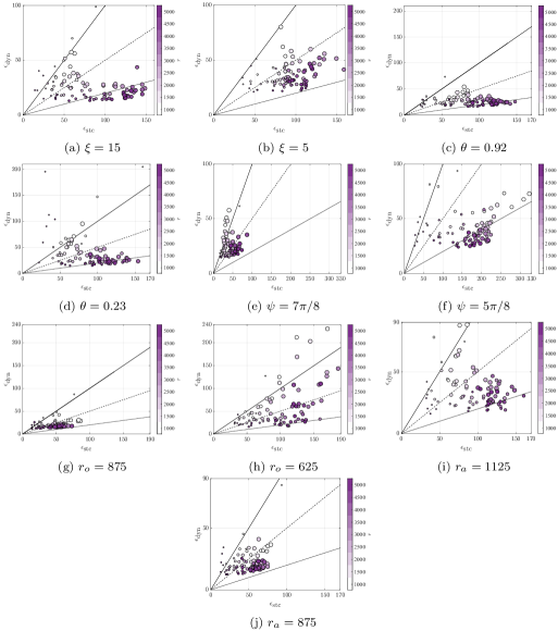
Figure 9: Comparison of asymptotic cumulative tracking errors $\epsilon_{\operatorname{stc}}$ and $\epsilon_{\operatorname{dyn}}$. Each circle represents data from performing 100 control trials for a fixed pair $(N,r_{{\operatorname{ref}}})$. The area of each circle is proportional to $N$. The colors of markers represent $r_{{\operatorname{ref}}}$. Solid, dashed, and dotted lines represent the straight lines $\epsilon_{\operatorname{dyn}}=\epsilon_{\operatorname{stc}}$, $\epsilon_{\operatorname{stc}}/2$, and $\epsilon_{\operatorname{stc}}/5$, respectively. Overall, errors from the dynamic weight-model are smaller than the ones from the static weight-model for most cases.

5.3 Discussion

We investigated the reduced-order MPC of the fish schooling model reported by Gautrais et al. [19]. For the schooling model, we proposed reduced-order models based on the weighted average of the directions of individual fish. We then carefully analyzed the reduction errors, which suggested that the normalized eigenvector centrality of the alignment-interaction network within the school lead to better MPC. Finally, this finding and numerical efficiency of the MPC based on reduced-order models are confirmed by extensive simulations, in which we considered various scenarios with different school sizes $N$ and the curvature of the reference set $\mathcal{R}$. Therefore, this paper expands the applicability of reduced-order nonlinear MPC [39, 40] to the fish schooling model. This paper also strengthens the existing connection [42, 43] between control and centrality measures.

Although bounds (22) and (33) on the approximation errors suggest a robust MPC formulation [49], the current bounds do not directly allow us to employ such a formulation. The bounds do not allow us to evaluate the approximation error within the whole prediction horizon if its length is longer than one because error bounds (22) and (33) are not closed in the variable $\langle V\rangle_{\alpha}$ (i.e., $\hat{V}$) within the prediction model. Further, the current error bounds do not enable us to formulate MPC with a guaranteed tracking performance. To incorporate the error bounds into the MPC, it is necessary to derive other error bounds closed in the variable $\langle V\rangle_{\alpha}$.

Toward future application of the proposed method for the control of actual fish schools, it is important to analyze the robustness of the method against external disturbances and model uncertainties that are common in practice. For the disturbances, random rotations incorporated into the current model can be considered to represent external disturbances with relatively short time constants. Furthermore, we confirmed the effectiveness of the proposed method for the model whose magnitude of random rotation is set as ten times large as the parameter adopted in the original model [19]. Therefore, the proposed method has a certain degree of robustness against external disturbances with small time constants. On the other hand, analyzing robustness of the proposed method to external disturbances with long time constants, such as unexpected steady flow in water, remains an open problem. Likewise, analysis of robustness to model uncertainties is not discussed in this paper. Performing such analysis and clarifying the proposed method’s sensitivity with respect to parameter errors is important because the sensitivity indicates which parameter needs to be correctly identified to obtain better control performance.

We finally remark the limited applicability of the proposed prediction models for small-scale fish schools although the control of small-scale schools is not within the scope of the current research. We numerically observed the violation of the connectivity condition $n_{i}>0$ in (20) when controlling small-scale schools, typically for those with less than 20 individuals. We found that this phenomenon occurs because of poor connectivity within small-scale schools. We leave the development of a reduced-order prediction model without requiring condition (20) as an open problem.

6 Conclusion

We studied the MPC of fish schools. We presented a reduced-order prediction model based on the weighted sum of directions with the weight being the normalized eigenvector centrality of the orientation-based attraction network in the fish school. We then numerically confirmed the effectiveness of the MPC with the reduced-order model. The proposed approach allowed the control of the fish school with hundreds of individuals and achieved smaller tracking errors than the MPC with the reduce-order model based on uniform weights.

There exist several future research directions that should be pursued. A research direction of practical importance is realizing reduced-order MPC with a guaranteed tracking performance, as such MPC is difficult to perform with the proposed prediction model. Another practically important research direction is generalization for the MPC of higher-order variables because the proposed method is limited to the control of the center of mass. Such a generalization would allow us to achieve complex fish behaviors such as milling. More realistic models of fish schooling such as the one in [50] that can account for water flows also need to be considered. From the theoretical side, it is important to examine the generalizability of the current reduction approach to other swarm models.

Appendix A Proof of Theorem 4.1

For the ease of presentation, we omit the time variable $k$ if no confusion is expected. We start by proving the following technical lemma on the normalization operator $\phi$ defined in (5).

Lemma A.1.

For all $x,y\in\mathbb{R}^{3}$ such that $x\neq 0$ and $x+y\neq 0$, define

$${\delta\phi(x,y)=\phi(x+y)-\left(\phi(x)+\frac{1}{\lVert x\rVert}y-\frac{y^{\top}x}{\lVert x\rVert^{3}}x\right).}$$ (36)

Then,

$${\lVert\delta\phi(x,y)\rVert\leq\frac{2}{\lVert x\rVert^{2}}\lVert y\rVert^{2}}$$ (37)

for all $x\neq 0$ and $y\in\mathbb{R}^{3}\backslash\{-x\}$.

Proof.

Let us first consider the the special case of $x=e_{1}$, where $e_{1}=[1\ 0\ 0]^{\top}$ denotes the first element of the canonical basis of $\mathbb{R}^{3}$. Let $y\in\mathbb{R}^{3}\backslash\{-x\}$ be arbitrary. Define $z=y+x$ and let $z_{1}$, $z_{2}$, and $z_{3}$ denote the first, second, and third entries of vector $z$, respectively. Because $\lVert x\rVert=\lVert e_{1}\rVert=1$, $y=z-e_{1}$, and $\delta\phi(x,y)=\phi(z)-[1\ z_{2}\ z_{3}]^{\top}$, to prove the lemma, we show

$$\lVert\phi(z)-[1\ z_{2}\ z_{3}]^{\top}\rVert^{2}\leq 4\lVert z-e_{1}\rVert^{4}$$ (38)

for all nonzero $z$.

Let us write $R=\lVert z\rVert$ and $r=z_{1}$. Then, an algebraic manipulation shows

$$\lVert\phi(z)-[1\ z_{2}\ z_{3}]^{\top}\rVert^{2}=2+R^{2}-r^{2}-2\frac{R^{2}-r^{2}+r}{R}$$ (39)

and

$$\lVert z-e_{1}\rVert^{4}=(R^{2}-2r+1)^{2}.$$ (40)

Because $r$ can take any value within the interval $[-R,R]$, we introduce an auxiliary variable $s\in[-1,1]$ and write $r=sR$. Then, using equations (39) and (40), we can show that the difference $\Delta=4\lVert z-e_{1}\rVert^{4}-\lVert\phi(z)-[1\ z_{2}\ z_{3}]^{\top}\rVert^{2}$ admits the representation

$$\Delta=a(R)s^{2}+b(R)s+c(R),$$

where $a(R)=17R^{2}-2R$, $b(R)=-16R^{3}-16R+2$, and $c(R)=4R^{4}+3R^{2}+2$. Therefore, to prove (38), we need to show that $\Delta\geq 0$ holds for all $R\geq 0$ and $s\in[-1,1]$. Let us first consider the case $R\leq 1/4$. In this case, because $c(R)\geq 0$, we have $\Delta\geq-\lvert a(R)\rvert-\lvert b(R)\rvert+c(R)$. We can show that function $R\mapsto{-\lvert a(R)\rvert-\lvert b(R)\rvert+c(R)}$ is nonnegative on the interval $[0,1/4]$, and therefore, we conclude that $\Delta\geq 0$ holds for all $s$. Next, let us consider the case $R\geq 1/4$. In this case, we can show that $a(R)>0$ and $b(R)^{2}-4a(R)c(R)\leq 0$. This shows that $\Delta$, as a quadratic function of $s$, is nonnegative. This observation implies $\Delta\geq 0$ for the case $R\geq 1/4$ as well. Hence, we showed that (37) holds if $x=e_{1}$ for all $y\neq e_{1}$

Let us consider a general $x$. Take an orthogonal matrix $M$ such that $x=\lVert x\rVert{M}e_{1}$. A simple calculation shows $\delta\phi(x,y)=M\,\delta\phi(e_{1},\lVert x\rVert^{-1}{M}^{\top}y)$. Therefore, we can show

$$\lVert\delta\phi(x,y)\rVert =\left\lVert\delta\phi(e_{1},\lVert x\rVert^{-1}{M}^{\top}y)\right\rVert$$

$$\leq 2\left\lVert\lVert x\rVert^{-1}{M}^{\top}y\right\rVert^{2}$$

$$=({2}/{\lVert x\rVert^{2}})\lVert y\rVert^{2},$$

as desired. ∎

We also prove the following lemma.

Lemma A.2.

For all $i\in\{1,\dotsc,N\}$, the vector

$$\delta_{\alpha}O_{i}=O_{i}-n_{i}\langle V\rangle_{\alpha}$$

satisfies

$$\lVert\delta_{\alpha}O_{i}\rVert\leq n_{i}\sqrt{Q_{i,n_{i}\alpha}}.$$ (41)

Proof.

For all $i,j\in\{1,\dotsc,N\}$, define $\sigma_{ij}=1-V_{i}^{\top}V_{j}$. Definition (3) of the vector $O_{i}$ shows $\delta_{\alpha}O_{i}=\sum_{j=1}^{N}(\omega_{ij}-n_{i}\alpha_{j})V_{j}$. Therefore,

$$\lVert\delta_{\alpha}O_{i}\rVert^{2}=-\sum_{j=1}^{N}\sum_{j^{\prime}=1}^{N}(\omega_{ij}-n_{i}\alpha_{j})(\omega_{ij^{\prime}}-n_{i}\alpha_{j^{\prime}})\sigma_{jj^{\prime}},$$ (42)

where we use equality $\sum_{j=1}^{N}(\omega_{ij}-n_{i}\alpha_{j})=0$. Therefore, equation (42) and the trivial inequality $\sigma_{ij}\leq\theta_{ij}^{2}/2$ prove $\lVert\delta_{\alpha}O_{i}\rVert^{2}\leq\sum_{j=1}^{N}\sum_{j^{\prime}=1}^{N}\lvert\omega_{ij^{\prime}}-n_{i}\alpha_{j^{\prime}}\rvert\,\lvert\omega_{ij}-n_{i}\alpha_{j}\rvert\theta_{jj^{\prime}}^{2}/2=n_{i}^{2}Q_{i,n_{i}\alpha}$, as desired. ∎

Using Lemmas A.1 and A.2, we prove the following preliminary error-bound for proving Theorem 4.1.

Proposition A.3.

Let $i\in\{1,\dotsc,N\}$. Assume that (20) holds. Define

$$w_{i}=\eta A_{i}+\xi_{i}u_{i}.$$ (43)

If $\langle V\rangle_{\alpha}\neq 0$, then the norm of the vector $\zeta_{i}$ defined by

$$\zeta_{i}=\phi(D_{i})-\left(\langle V\rangle_{\alpha}+\frac{w_{i}}{n_{i}}-\frac{w_{i}^{\top}\langle V\rangle_{\alpha}}{n_{i}\lVert\langle V\rangle_{\alpha}\rVert^{2}}\langle V\rangle_{\alpha}\right)$$ (44)

satisfies

$$\begin{multlined}\lVert\zeta_{i}\rVert\leq 2\tilde{\pi}_{\alpha}\rho_{i}+2\rho_{i}^{2}+\tilde{\pi}_{i}(1+4\rho_{i})+(1+2\rho_{i})\sqrt{Q_{i,n_{i}\alpha}}.\end{multlined}\lVert\zeta_{i}\rVert\leq 2\tilde{\pi}_{\alpha}\rho_{i}+2\rho_{i}^{2}+\tilde{\pi}_{i}(1+4\rho_{i})+(1+2\rho_{i})\sqrt{Q_{i,n_{i}\alpha}}.$$

Proof.

Let us first show that the vector $\zeta_{i}$ can be decomposed as

$$\zeta_{i}=\zeta_{i,1}+\zeta_{i,2}+\zeta_{i,3}+\zeta_{i,4}+\zeta_{i,5}+\zeta_{i,6},$$ (45)

where vectors $\zeta_{i,1}$, …, $\zeta_{i,6}$ are defined by

$$\zeta_{i,1} =\delta\phi(O_{i},w_{i}),$$

$$\zeta_{i,2} =\phi(O_{i})-\langle V\rangle_{\alpha},$$

$$\zeta_{i,3} =({\lVert O_{i}\rVert^{-1}-n_{i}^{-1}})w_{i},$$

$$\zeta_{i,4} =-(\lVert O_{i}\rVert^{-3}-n_{i}^{-3})(w_{i}^{\top}O_{i})O_{i},$$

$$\zeta_{i,5} =\frac{w_{i}^{\top}\langle V\rangle_{\alpha}}{n_{i}\lVert\langle V\rangle_{\alpha}\rVert^{2}}\langle V\rangle_{\alpha}-\frac{w_{i}^{\top}\langle V\rangle_{\alpha}}{n_{i}}\langle V\rangle_{\alpha},$$

$$\zeta_{i,6} =\frac{w_{i}^{\top}\langle V\rangle_{\alpha}}{n_{i}}\langle V\rangle_{\alpha}-\frac{w_{i}^{\top}O_{i}}{n_{i}^{3}}O_{i}.$$

By definition (36) of the mapping $\delta\phi$ and identity $D_{i}=O_{i}+w_{i}$, we can show $\delta\phi(O_{i},w_{i})+\phi(O_{i})+\lVert O_{i}\rVert^{-1}w_{i}-\lVert O_{i}\rVert^{-3}(w_{i}^{\top}O_{i})O_{i}=\phi(O_{i}+w_{i})=\phi(D_{i})$. Therefore, a simple algebraic manipulation yields

$$\zeta_{i,1}+\zeta_{i,2}+\zeta_{i,3}+\zeta_{i,4}=\phi(D_{i})-\langle V\rangle_{\alpha}-n^{-1}w_{i}+n_{i}^{-3}(w_{i}^{\top}O_{i})O_{i}.$$

We can also easily see that

$$\zeta_{i,5}+\zeta_{i,6}=\frac{w_{i}^{\top}\langle V\rangle_{\alpha}}{n_{i}\lVert\langle V\rangle_{\alpha}\rVert^{2}}\langle V\rangle_{\alpha}-\frac{w_{i}^{\top}O_{i}}{n_{i}^{3}}O_{i}.$$

Hence, from (44), we can confirm the decomposition (45), as required.

Next, let us evaluate the norm of each of these vectors. Lemma A.1 shows

$$\lVert\zeta_{i,1}\rVert \leq 2\lVert O_{i}\rVert^{-2}\lVert w_{i}\rVert^{2}=4\rho_{i}^{2}.$$ (46)

Because $\zeta_{i,2}=(\lVert O_{i}\rVert^{-1}-n_{i}^{-1})O_{i}-n_{i}^{-1}\delta_{\alpha}O_{i}$, inequality (41) shows

$$\lVert\zeta_{i,2}\rVert \leq(\lVert O_{i}\rVert^{-1}-n_{i}^{-1})\lVert O_{i}\rVert+\sqrt{Q_{i,n_{i}\alpha}}$$ (47)

$$=\tilde{\pi}_{i}+\sqrt{Q_{i,n_{i}\alpha}}.$$

Similarly, we can show

$$\lVert\zeta_{i,3}\rVert \leq({\lVert O_{i}\rVert^{-1}-n_{i}^{-1}})\lVert w_{i}\rVert=\tilde{\pi}_{i}\rho_{i},$$ (48)

and

$$\lVert\zeta_{i,4}\rVert \leq(\lVert O_{i}\rVert^{-3}-n_{i}^{-3})\lVert w_{i}\rVert\lVert O_{i}\rVert^{2}$$ (49)

$$=\rho_{i}(1-\pi_{i}^{3})$$

$$\leq 3\tilde{\pi}_{i}\rho_{i}.$$

Furthermore, it follows that

$$\lVert\zeta_{i,5}\rVert \leq(1-\lVert\langle V\rangle_{\alpha}\rVert^{2})\lVert w_{i}\rVert n_{i}^{-1}$$ (50)

$$\leq 2\tilde{\pi}_{\alpha}\rho_{i}.$$

By using the triangle inequality and inequality (41), we can show

$$\lVert\zeta_{i,6}\rVert \leq 2\lVert w_{i}\rVert n_{i}^{-1}\sqrt{Q_{i,n_{i}\alpha}}$$ (51)

$$\leq 2\rho_{i}\sqrt{Q_{i,n_{i}\alpha}}.$$

Finally, inequalities 46, 47, 48, 49, 50 and 51 complete the proof. ∎

We can now prove Theorem 4.1. Let $w=A+u$. From definition (43) of vector $w_{i}$, we have $\sum_{i=1}^{N}({\alpha_{i}}/{n_{i}})w_{i}=w$. Therefore, taking the weighted summation with respect to $i$ in equation (44) shows

$$\langle\zeta\rangle_{\alpha} =\begin{multlined}\langle\phi(D)\rangle_{\alpha}-\left(\langle V\rangle_{\alpha}+w-\frac{w^{\top}\langle V\rangle_{\alpha}}{\lVert\langle V\rangle_{\alpha}\rVert^{2}}\langle V\rangle_{\alpha}\right)\end{multlined}\langle\phi(D)\rangle_{\alpha}-\left(\langle V\rangle_{\alpha}+w-\frac{w^{\top}\langle V\rangle_{\alpha}}{\lVert\langle V\rangle_{\alpha}\rVert^{2}}\langle V\rangle_{\alpha}\right)$$

$$=\begin{multlined}\langle\phi(D)\rangle_{\alpha}-\lVert\langle V\rangle_{\alpha}\rVert\,\phi\bigl{(}\langle V\rangle_{\alpha}+w\bigr{)}+\lVert\langle V\rangle_{\alpha}\rVert\,\delta\phi\bigl{(}\langle V\rangle_{\alpha},w\bigr{)},\end{multlined}\langle\phi(D)\rangle_{\alpha}-\lVert\langle V\rangle_{\alpha}\rVert\,\phi\bigl{(}\langle V\rangle_{\alpha}+w\bigr{)}+\lVert\langle V\rangle_{\alpha}\rVert\,\delta\phi\bigl{(}\langle V\rangle_{\alpha},w\bigr{)},$$

where in the last equation we used (36). Therefore,

$$\epsilon_{\alpha}=\langle\zeta\rangle_{\alpha}-\lVert\langle V\rangle_{\alpha}\rVert\,\delta\phi\bigl{(}\langle V\rangle_{\alpha},w\bigr{)}.$$ (52)

Hence, the triangle inequality as well as Proposition A.3 and Lemma A.1 complete the proof of inequality (22).

Appendix Appendix B Proof of Theorem 4.4

Define vector $\zeta_{i}$ as in (44). Assume that $\alpha$ equals the normalized eigenvector centrality of $\mathcal{G}_{o}(k)$. Let us decompose vector $\langle\zeta\rangle_{\alpha}=\sum_{i=1}^{N}\alpha_{i}\zeta_{i}$ as $\langle\zeta\rangle_{\alpha}=\omega_{1}+\omega_{2}+\omega_{3}+\omega_{4}+\omega_{5}+\omega_{6}$, where $\omega_{\ell}=\sum_{i=1}^{N}\alpha_{i}\zeta_{i,\ell}$ for all $\ell=1,\dotsc,6$. We bound the norm of vectors $\omega_{1}$, $\omega_{3}$, $\omega_{4}$, $\omega_{5}$, and $\omega_{6}$ using inequalities (46) and (48)–(51). Let us evaluate $\lVert\omega_{2}\rVert$ in a different manner. Because $\alpha$ is assumed to be equal to the normalized eigenvector centrality of $\mathcal{G}_{o}(k)$, from equation (32) we can show

$$\omega_{2}=\sum_{i=1}^{N}\alpha_{i}(\phi(O_{i})-\langle V\rangle_{\alpha})=\sum_{i=1}^{N}\alpha_{i}(\phi(O_{i})-n_{i}^{-1}O_{i}).$$

Thus, we obtain $\lVert\omega_{2}\rVert\leq\sum_{i=1}^{N}\alpha_{i}\tilde{\pi}_{i}$. This inequality as well as inequalities (46) and (48)–(51) show

$$\begin{multlined}\lVert\langle\zeta\rangle_{\alpha}\rVert\leq\sum_{i=1}^{N}\alpha_{i}\bigg{(}2\tilde{\pi}_{\alpha}\rho_{i}+2\rho_{i}^{2}+\tilde{\pi}_{i}(1+4\rho_{i})+2\rho_{i}\sqrt{Q_{i,n_{i}\alpha}}\bigg{)}.\end{multlined}\lVert\langle\zeta\rangle_{\alpha}\rVert\leq\sum_{i=1}^{N}\alpha_{i}\bigg{(}2\tilde{\pi}_{\alpha}\rho_{i}+2\rho_{i}^{2}+\tilde{\pi}_{i}(1+4\rho_{i})+2\rho_{i}\sqrt{Q_{i,n_{i}\alpha}}\bigg{)}.$$

Therefore, equality (52) as well as Proposition A.3 and Lemma A.1 complete the proof of the theorem, as desired.

References

- [1] M. Perc, P. Grigolini, Collective behavior and evolutionary games - An introduction, Chaos, Solitons and Fractals 56 (2013) 1–5.
- [2] N. E. Leonard, Multi-agent system dynamics: Bifurcation and behavior of animal groups, Annual Reviews in Control 38 (2014) 171–183.
- [3] J. L. Burton, N. R. Franks, The foraging ecology of the army ant Eciton rapax: an ergonomic enigma?, Ecological Entomology 10 (1985) 131–141.
- [4] J. T. Emlen, Flocking behavior in birds, The Auk 69 (1952) 160–170.
- [5] J. K. Parrish, S. V. Viscido, D. Grünbaum, Self-organized fish schools: An examination of emergent properties, Biological Bulletin 202 (2002) 296–305.
- [6] C. Feliciani, K. Nishinari, Empirical analysis of the lane formation process in bidirectional pedestrian flow, Physical Review E 94 (2016) 032304.
- [7] A. Berdahl, A. van Leeuwen, S. A. Levin, C. J. Torney, Collective behavior as a driver of critical transitions in migratory populations, Movement Ecology 4 (2016) 18.
- [8] J. Kennedy, R. Eberhart, Particle swarm optimization, in: 1995 IEEE International Conference on Neural Networks, 1995, pp. 1942–1948.
- [9] M. Brambilla, E. Ferrante, M. Birattari, M. Dorigo, Swarm robotics: A review from the swarm engineering perspective, Swarm Intelligence 7 (2013) 1–41.
- [10] S. Mayya, P. Pierpaoli, G. Nair, M. Egerstedt, Localization in densely packed swarms using interrobot collisions as a sensing modality, IEEE Transactions on Robotics 35 (2019) 21–34.
- [11] R. Gray, A. Franci, V. Srivastava, N. E. Leonard, Multiagent decision-making dynamics inspired by honeybees, IEEE Transactions on Control of Network Systems 5 (2018) 793–806.
- [12] L. Stella, D. Bauso, Bio-inspired evolutionary dynamics on complex networks under uncertain cross-inhibitory signals, Automatica 100 (2019) 61–66.
- [13] M. Jusup, P. Holme, K. Kanazawa, M. Takayasu, I. Romić, Z. Wang, S. Geček, T. Lipić, B. Podobnik, L. Wang, W. Luo, T. Klanjšček, J. Fan, S. Boccaletti, M. Perc, Social physics, Physics Reports 948 (2022) 1–148.
- [14] M. Perc, J. J. Jordan, D. G. Rand, Z. Wang, S. Boccaletti, A. Szolnoki, Statistical physics of human cooperation, Physics Reports 687 (2017) 1–51.
- [15] A. Huth, C. Wissel, The simulation of the movement of fish schools, Journal of Theoretical Biology 156 (1992) 365–385.
- [16] I. D. Couzin, J. Krause, R. James, G. D. Ruxton, N. R. Franks, Collective memory and spatial sorting in animal groups, Journal of Theoretical Biology 218 (2002) 1–11.
- [17] H. Kunz, C. K. Hemelrijk, Artificial fish schools: Collective effects of school size, body size, and body form, Artificial Life 9 (2003) 237–253.
- [18] S. V. Viscido, J. K. Parrish, D. Grünbaum, Individual behavior and emergent properties of fish schools: A comparison of observation and theory, Marine Ecology Progress Series 273 (2004) 239–250.
- [19] J. Gautrais, C. Jost, G. Theraulaz, Key behavioural factors in a self-organised fish school model, Annales Zoologici Fennici 45 (2008) 415–428.
- [20] D. S. Calovi, U. Lopez, P. Schuhmacher, H. Chaté, C. Sire, G. Theraulaz, Collective response to perturbations in a data-driven fish school model, Journal of The Royal Society Interface 12 (2015) 20141362.
- [21] J. B. Poletto, D. E. Cocherell, T. D. Mussen, A. Ercan, H. Bandeh, M. L. Kavvas, J. J. Cech, N. A. Fangue, Fish-protection devices at unscreened water diversions can reduce entrainment: Evidence from behavioural laboratory investigations, Conservation Physiology 3 (2015) cov040.
- [22] M. Virgili, C. Vasapollo, A. Lucchetti, Can ultraviolet illumination reduce sea turtle bycatch in Mediterranean set net fisheries?, Fisheries Research 199 (2018) 1–7.
- [23] A. Bielli, J. Alfaro-Shigueto, P. D. Doherty, B. J. Godley, C. Ortiz, A. Pasara, J. H. Wang, J. C. Mangel, An illuminating idea to reduce bycatch in the Peruvian small-scale gillnet fishery, Biological Conservation 241 (2020) 108277.
- [24] C. J. Filho, F. B. de Lima Neto, A. J. Lins, A. I. Nascimento, M. P. Lima, Fish school search, Studies in Computational Intelligence 193 (2009) 261–277.
- [25] R. Olfati-Saber, Flocking for multi-agent dynamic systems: Algorithms and theory, IEEE Transactions on Automatic Control 51 (2006) 401–420.
- [26] W. Li, Stability analysis of swarms with general topology, IEEE Transactions on Systems, Man, and Cybernetics, Part B: Cybernetics 38 (2008) 1084–1097.
- [27] K. Bakshi, D. D. Fan, E. A. Theodorou, Schrodinger approach to optimal control of large-size populations, IEEE Transactions on Automatic Control 66 (2020) 2372–2378.
- [28] D. A. Paley, N. E. Leonard, R. Sepulchre, D. Grunbaum, J. K. Parrish, Oscillator models and collective motion, IEEE Control Systems Magazine 27 (2007) 89–105.
- [29] X. Li, Z. Cai, J. Xiao, Stable swarming by mutual interactions of attraction/alignment/repulsion: fixed topology, in: 17th IFAC World Congress, 2008, pp. 5143–5148.
- [30] J. Rossiter, Model-Based Predictive Control, CRC Press, 2017.
- [31] N. S. Richards, S. R. Chipps, M. L. Brown, Stress response and avoidance behavior of fishes as influenced by high-frequency strobe lights, North American Journal of Fisheries Management 27 (2007) 1310–1315.
- [32] C. K. Elvidge, C. H. Reid, M. I. Ford, M. Sills, P. H. Patrick, D. Gibson, S. Backhouse, S. J. Cooke, Ontogeny of light avoidance in juvenile lake sturgeon, Journal of Applied Ichthyology 35 (2019) 202–209.
- [33] M. Marchesan, M. Spoto, L. Verginella, E. A. Ferrero, Behavioural effects of artificial light on fish species of commercial interest, Fisheries Research 73 (2005) 171–185.
- [34] M. I. Ford, C. K. Elvidge, D. Baker, T. C. Pratt, K. E. Smokorowski, M. Sills, P. Patrick, S. J. Cooke, Preferences of age-0 white sturgeon for different colours and strobe rates of LED lights may inform behavioural guidance strategies, Environmental Biology of Fishes 101 (2018) 667–674.
- [35] J. Kim, C. Bondy, C. M. Chandler, N. E. Mandrak, Behavioural response of juvenile common carp (Cyprinus carpio) and juvenile channel catfish (Ictalurus punctatus) to strobe light, Fishes 4 (2019) 29.
- [36] S. Hovland, C. Løvaas, J. T. Gravdahl, G. C. Goodwin, Stability of model predictive control based on reduced-order models, in: 47th IEEE Conference on Decision and Control, 2008, pp. 4067–4072.
- [37] M. Löhning, M. Reble, J. Hasenauer, S. Yu, F. Allgöwer, Model predictive control using reduced-order models: Guaranteed stability for constrained linear systems, Journal of Process Control 24 (2014) 1647–1659.
- [38] J. Lorenzetti, A. McClellan, C. Farhat, M. Pavone, Linear reduced-order model predictive control, IEEE Transactions on Automatic Control 67 (2022) 5980–5995.
- [39] A. P. Wiese, M. J. Blom, C. Manzie, M. J. Brear, A. Kitchener, Model reduction and MIMO model predictive control of gas turbine systems, Control Engineering Practice 45 (2015) 194–206.
- [40] A. Zhang, J. Liu, Economic MPC of wastewater treatment plants based on model reduction, Processes 7 (2019) 682.
- [41] P. Boldi, S. Vigna, Axioms for centrality, Internet Mathematics 10 (2014) 222–262.
- [42] Y.-Y. Liu, J.-J. Slotine, A.-L. Barabási, Control centrality and hierarchical structure in complex networks, PLoS ONE 7 (2012) e44459.
- [43] K. Fitch, N. Ehrich Leonard, Joint centrality distinguishes optimal leaders in noisy networks, IEEE Transactions on Control of Network Systems 3 (2016) 366–378.
- [44] A. Bayen, R. Raffard, C. Tomlin, Adjoint-based control of a new eulerian network model of air traffic flow, IEEE Transactions on Control Systems Technology 14 (2006) 804–818.
- [45] S. A. Kumar, J. Vanualailai, B. Sharma, A. Prasad, Velocity controllers for a swarm of unmanned aerial vehicles, Journal of Industrial Information Integration 22 (2021) 100198.
- [46] S. A. Kumar, B. Sharma, J. Vanualailai, A. Prasad, Stable switched controllers for a swarm of UGVs for hierarchal landmark navigation, Swarm and Evolutionary Computation 65 (2021) 100926.
- [47] C. W. Reynolds, Flocks, herds, and schools: A distributed behavioral model, in: 14th Annual Conference on Computer Graphics and Interactive Techniques, 1987, pp. 25–34.
- [48] T. Vicsek, A. Czirók, E. Ben-Jacob, I. Cohen, O. Shochet, Novel type of phase transition in a system of self-driven particles, Physical Review Letters 75 (1995) 1226–1229.
- [49] D. Mayne, Robust and stochastic model predictive control: Are we going in the right direction?, Annual Reviews in Control 41 (2016) 184–192.
- [50] A. Filella, F. Nadal, C. Sire, E. Kanso, C. Eloy, Model of collective fish behavior with hydrodynamic interactions, Physical Review Letters 120 (2018) 198101.