Traffic State Estimation with Anisotropic Gaussian Processes from Vehicle Trajectories

Abstract

Accurately monitoring road traffic state and speed is crucial for various applications, including travel time prediction, traffic control, and traffic safety. However, the lack of sensors often results in incomplete traffic state data, making it challenging to obtain reliable information for decision-making. This paper proposes a novel method for imputing traffic state data using Gaussian processes (GP) to address this issue. We propose a kernel rotation re-parametrization scheme that transforms a standard isotropic GP kernel into an anisotropic kernel, which can better model the propagation of traffic waves in traffic flow data. This method can be applied to impute traffic state data from fixed sensors or probe vehicles. Moreover, the rotated GP method provides statistical uncertainty quantification for the imputed traffic state, making it more reliable. We also extend our approach to a multi-output GP, which allows for simultaneously estimating the traffic state for multiple lanes. We evaluate our method using real-world traffic data from the Next Generation simulation (NGSIM) and HighD programs. Considering current and future mixed traffic of connected vehicles (CVs) and human-driven vehicles (HVs), we experiment with the traffic state estimation scheme from 5% to 50% available trajectories, mimicking different CV penetration rates in a mixed traffic environment. Results show that our method outperforms state-of-the-art methods in terms of estimation accuracy, efficiency, and robustness.

I Introduction

Intelligent transportation systems (ITS) rely heavily on traffic state information, which is typically collected using a variety of detectors, such as loop detectors, video cameras, probe vehicles, and, more recently, connected vehicles (CVs). However, each type of detector has its limitations in terms of coverage and completeness of data. For instance, loop detectors are stationary sensors that only provide data at fixed locations, while video cameras require significant time and resources to process footage and must be installed on a high building or a gantry. As a result, these sensors are sparsely distributed in the traffic network, resulting in limited spatial coverage. In recent years, mobile sensors such as probe vehicles and CVs that can provide real-time traffic information, including speed and location, are playing an ever-important role in TSE. However, because of the low penetration rate of CVs, the trajectories of CVs is sparse in both space and time. Therefore, an imputation method is needed to obtain the traffic state information in the entire spatiotemporal space, which would enable more accurate traffic control and management in ITS.

Traffic state estimation (TSE) refers to the inference of traffic state variables, such as density, speed, or other relevant variables, in a spatiotemporal domain by utilizing partially observed traffic data from detectors [1]. Generally, there are two types of TSE approaches: model-based and data-driven. Model-based TSE methods rely on traffic flow models and require strong prior knowledge, such as the capacity of the road, to accurately infer traffic state variables. Typical methods include first-order Lighthill-Whitham-Richards (LWR) model [2, 3] and high-order Payne-Whitham (PW) model [4, 5]. However, model-based TSE may not always be accurate because it may not fully capture the complexity of real-world traffic. Conversely, with massive traffic data and machine learning techniques available, TSE can be achieved in a purely data-driven manner, as demonstrated by some recent works [6, 7]. However, the training of a data-driven approach typically requires a large external training dataset and a validation dataset with full information. For example, many deep-learning-based TSE models [7] are first trained on a traffic simulation dataset, and then applied to a real-world TSE problem. However, it may not always be possible to obtain an appropriate training dataset, and the external dataset may not be representative of the road segment with missing values. Therefore, there is a need to develop a data-driven TSE method without any external training dataset. For cases where the observed data is extremely sparse, we expect the TSE could also be able to provide statistical uncertainty quantification for the estimation.

To address the above research gap, we propose using Gaussian processes (GPs) [8] for TSE. GPs are non-parametric Bayesian models that have been widely used for spatiotemporal kriging/imputation, providing a data-driven TSE approach that does not require an external training dataset. Additionally, GPs offer statistical uncertainty quantification for TSE. However, conventional GP models are inadequate in modeling traffic flow data due to the non-stationarity and anisotropy caused by traffic wave propagation. Taking Fig. 2 (a) as an example, the congestion wave propagates backward, generating directional spatiotemporal correlations that traditional GP kernels cannot model. To capture the anisotropic correlation in traffic wave propagation, we re-parameterized the GP kernel with a rotation angle. The kernel rotation angle indicates the speed of congestion propagation in traffic waves and can be estimated from partially observed data. We address the scalability issue of the GP model with variational sparse GP. Moreover, we propose using a multi-output GP model to simultaneously enable TSE on multiple lanes, rather than using several individual GPs. To test the TSE performance, we compare the proposed rotated GP with other imputation methods in NGSIM and highD datasets under a wide range of percentages of observed traffic information, which can also be regarded as CV penetration rates in the mixed traffic environment. Experimental results demonstrate that the proposed rotated GP significantly outperforms other methods regarding accuracy and robustness for TSE under low CV penetration rates.

The contributions of this paper are summarized as follows:

• A new approach is proposed for TSE using Gaussian process (GP) models with rotated anisotropic kernels that can capture the anisotropic correlation in traffic wave propagation. The rotation angle can be estimated from partially observed data and provides insight into the speed of congestion propagation in traffic waves.

• The proposed GP-based TSE method is a purely data-driven approach that does not require an external training dataset and provides statistical uncertainty quantification for the estimation, which is important for TSE under low CV penetration rates.

• The multi-output GP model is proposed for TSE on multiple lanes, which leverages the correlation between the traffic states of different lanes to improve TSE accuracy.

• Extensive experiments on two real-world datasets and different CV penetration rates demonstrate that the proposed GP-based TSE method outperforms other state-of-the-art methods in terms of accuracy and robustness.

The remainder of the paper is organized as follows. We review related work on TSE in Section II. In Section III, we describe the problem and the proposed method. The experimental settings and results are presented in Section IV. Finally, we conclude the paper and discuss future research directions in Section V.

II Related work

We can broadly classify existing traffic state estimation (TSE) models into model-based and data-driven methods, specifically model-based, data-driven, and streaming data-driven strategies [1]. Model-based approaches adopt microscopic traffic flow models mathematically to depict the traffic states; these models include first-order traffic models like the Lighthill-Whitham-Richards (LWR) model [2, 3], high-order traffic models like Payne-Whitham (PW) model [4, 5] and the Aw-Rascle-Zhang (ARZ) model [9, 10, 11], and their extensions. The model-based approach often performs the Data Assimilation (DA) or estimation with the traffic observation via the filter-based method. The most utilized one is the Kalman filter (KF) and its variants - KF-like techniques (e.g., the extended/unscented/ensembled Kalman filter) [12, 13, 14, 15, 16, 17]. Other methods are not oriented from the Kalman filter, such as particle filter (PF) [18], adaptive smoothing filter (ASF) [19], or others. A comprehensive review of the above methods can be found in [1]. Although the model-based techniques can follow the traffic principles, these models rely a lot on the assumptions of traffic physics that can lead to numerical biases or approximation errors when the premises are not coherent with real-world data. In addition, model-based methods require substantial prior information on traffic dynamics.

Due to the availability of massive traffic data and the development of machine learning techniques, data-driven models get more attraction. Data-driven models usually utilize statistical or machine-learning approaches to infer traffic states from the spatiotemporal characteristics extracted from historical data (e.g., from sensors like loop detectors, cameras, or connected vehicles). For example, various research incorporates the spatiotemporal features into data-driven models utilizing the following techniques like the auto-regressive integrated moving average (ARIMA) [20], Bayesian network (BN) [21], Kernel regression (KR) [22], k-nearest neighbors (kNN) [23], convolutional neural networks (CNN) and deep neural networks (DNN) [24, 7, 25, 26, 27, 28], graph embedding generative adversarial network (GE-GAN) [29], tensor decomposition [6], and principal component analysis [30] et al. Besides, streaming-data-driven approaches are regarded as more robust against uncertainties while requiring a large amount of streaming data to perform the prediction. Some research contributes to the streaming-data-driven models, such as [31] and [32]. One of the advantages of data-driven models is that they require less prior info on traffic dynamics and can be more accurate than model-based methods. The other advantage is that they do not need rigid assumptions for traffic principles, which may cause unexplainable estimation. Meanwhile, the data-driven models often depend on a large amount of training data.

In terms of data sources. Most research discussed thus far utilized static data from fixed-location sensors like loop detectors or static data combined with mobile data obtained from probe vehicles [12, 33, 34]. Recently, more and more researchers investigated the trajectory-based TSE methods from the data. For example, utilized the trajectory data of probe vehicles or connected-automated vehicles (CAVs) to estimate the traffic state of freeways Seo et al. [35], Kyriacou et al. [36], Seo and Kusakabe [33], Wang et al. [6]. Moreover, there is a trend that combines model-based and data-driven models to develop “physics-informed” machine learning models for TSE [27, 37, 28].

Traditional fixed sensors are expensive to install and maintain throughout the road. With the development of Connected Vehicle (CV) technology, there exists an opportunity that such moving sensors can provide data sources at a relatively cheaper cost all over the road. Therefore, we still have to deal with the scenario where data is sparse because not all cars are CVs to provide information. There is some research about the TSE using CV technology. Chen and Levin [38] estimated traffic states like flow, density, and speed by proposing an algorithm based on CV Basic Safety Message (BSM) data. This study tested the Kalman Filter and cell transmission algorithm in a simulator. Fountoulakis et al. [39] proposed microscopic simulation research of the TSE with mixed traffic (CVs and conventional vehicles) via CV and spot-sensor data. At the same time, Bekiaris-Liberis et al. [40] developed a model-based TSE approach for per-lane density estimation and an on-ramp and off-ramp flow estimation in the presence of connected vehicles. There have also been works discussed online and offline TSE with CV data in a Bayesian model [36].

As presented here, the most similar research to our work is the adaptive smoothing interpolation (ASM) by Treiber et al. [41]. The authors used the anisotropic features of traffic waves and developed a smoothing method to estimate the traffic speed profile. However, their work lacks a well-defined method to determine the model parameters and the uncertainties of the estimation. In our study, the proposed GP approach is a probabilistic model that can learn the parameters and uncertainties from the data. Besides, the proposed method can be applied to the TSE problem with sparse data.

III Methodology

III-A Problem formulation

We aim to estimate the traffic state (speed in this paper) of a highway segment over a period of time, using data collected from fixed or moving sensors such as loop detectors and CVs. For a single lane of the highway segment, we denote $s$ as the spatial coordinate on the segment, $t$ as the temporal coordinate, and $y(s,t)$ as the traffic speed at location $s$ and time $t$. In practice, $s$ and $t$ are usually defined as discrete values on an $S\times T$ spatiotemporal grid. However, for our purposes, we can consider a general continuous space with a subscript $i$ such that $y_{i}=y(\mathbf{x}_{i})$, where $\mathbf{x}_{i}=[s_{i},t_{i}]^{\top}$ is a vector representing the spatiotemporal coordinate.

Assume we can obtain the traffic speed $\mathbf{y}_{o}=\left\{y_{i}\right\}_{i=1}^{n}$ at a set of spatiotemporal locations $X_{o}=\left\{\mathbf{x}_{i}\right\}_{i=1}^{n}$ using loop detectors or probe vehicles, where $n$ is the number of observations. Our goal is to estimate the traffic speed distribution $p\left(\mathbf{y}_{*}\right)$ at unknown spatiotemporal locations $X_{*}$ given the observed data $\left\{X_{o},\mathbf{y}_{o}\right\}$. For a highway segment with multiple lanes, the problem becomes estimating the joint distribution $p\left(\mathbf{y}^{1},\cdots,\mathbf{y}_{*}^{L}\right)$ from observations $\left\{X_{o}^{1},\mathbf{y}_{o}^{1},\cdots,X_{o}^{L},\mathbf{y}_{o}^{L}\right\}$, where $L$ is the number of lanes.

III-B Gaussian process regression

For a single lane of the highway segment, we assume the observed traffic state $y_{i}$ consists of a ground truth value $f_{i}$ and a noise term $\varepsilon_{i}$:

$$y_{i}=f_{i}+\varepsilon_{i},$$ (1)

where $\varepsilon$ is an independent and identically distributed (i.i.d.) Gaussian noise with zero mean and variance $\sigma_{\varepsilon}^{2}$.

Assume the ground truth traffic state $f$ is a function of the spatiotemporal coordinate $\mathbf{x}$. Next, we can impose a GP prior [8] to the function $f(\mathbf{x})\sim\mathcal{GP}\left(\mu,k\right)$, meaning any finite collection of $\mathbf{f}\in\mathbb{R}^{n}$ at $X$ has a joint Gaussian distribution:

$$\mathbf{f}=f(X)=\left[f(\mathbf{x}_{1}),\cdots,f(\mathbf{x}_{n})\right]^{\top}\sim\mathcal{N}(\bm{\mu},K),$$ (2)

where the mean is often set to be zero $\bm{\mu}=\mathbf{0}$, and the covariance matrix $K$ is defined by a kernel function $k$ such that $K\left[i,j\right]=k(\mathbf{x}_{i},\mathbf{x}_{j})$. For example, the commonly used squared exponential (SE) kernel takes the form:

$$k_{\mathrm{SE}}(\mathbf{x}_{i},\mathbf{x}_{j})=\sigma^{2}\exp\left(-\frac{1}{2\ell^{2}}\|\mathbf{x}_{i}-\mathbf{x}_{j}\|^{2}\right),$$ (3)

where the length scale $\ell$ determines how far apart two points in the input space can still be considered similar; the kernel variance $\sigma^{2}$ determines how far the function values can be from the mean. The kernel hyper-parameters and the noise variance $\bm{\theta}=\left\{\sigma^{2},\ell,\sigma_{\varepsilon}^{2}\right\}$ can be estimated from the observed data using Maximum Marginal likelihood (MML) estimation.

Taking advantage of the conditional Gaussian distribution, the posterior distribution of traffic state $\mathbf{f}_{*}$ at the unknown spatiotemporal locations $\mathbf{X}_{*}$ given observed data can be obtained by:

$$p\left(\mathbf{f}_{*}|X_{*},X_{o},\mathbf{y}_{o}\right) \sim\mathcal{N}\left(\bar{\mathbf{f}}_{*},\mathrm{cov}(\mathbf{f}_{*})\right),$$ (4)

$$\bar{\mathbf{f}}_{*} =K_{n*}^{\top}\left(K_{nn}+\sigma_{\varepsilon}^{2}I\right)^{-1}\mathbf{y}_{o},$$ (5)

$$\mathrm{cov}(\mathbf{f}_{*}) =K_{**}-K_{n*}^{\top}\left(K_{nn}+\sigma_{\varepsilon}^{2}I\right)^{-1}K_{n*},$$ (6)

where matrices $K_{nn}$, $K_{**}$, $K_{n*}$ represent the kernel evaluated at observed locations, unknown locations, and between observed and unknown locations, respectively. Next, the distribution of $\mathbf{y}_{*}$ can be readily obtained by Eq. (1).

III-C Rotated anisotropic kernel

Most GP kernels, such as the SE kernel in Eq. (3), are isotropic, meaning the covariance is only a function of $\|\mathbf{x}_{i}-\mathbf{x}_{j}\|$ and is invariant to the directions between $\mathbf{x}_{i}$ and $\mathbf{x}_{j}$. However, the traffic wave is anisotropic because the traffic wave propagates along a certain direction in the spatiotemporal grid. Although an isotropic kernel can have anisotropic properties by using different length scales on different dimensions (i.e., implementing automatic relevance determination (ARD) [42]), the ARD kernel is a very limited form and is still incapable of modeling the correlation propagates along a spatiotemporal direction.

Without loss of generality, let us consider the “squared distance” between $\mathbf{x}_{i}$ and $\mathbf{x}_{j}$ in an ARD kernel:

$$d(\mathbf{x}_{i},\mathbf{x}_{j})^{2}=(\mathbf{x}_{i}-\mathbf{x}_{j})^{\top}M(\mathbf{x}_{i}-\mathbf{x}_{j}),$$ (7)

where $M$ is a diagonal matrix with the $d$-th diagonal element being $\ell_{d}^{-2}$, specifying the dimension-specific length-scale. The diagonal structure of $M$ makes the length-scale along the spatial and temporal directions independent. To account for the traffic wave propagation, we introduce a rotation angle $\alpha$, a new hyper-parameters, which is the angle between the traffic wave and the space direction, as shown in Fig. 1. Then, we can measure the directional covariance using the following rotated squared distance: Then, we can measure the directional covariance using the following rotated squared distance:

$$\begin{split}d_{\mathrm{rot}}\left(\mathbf{x}_{i},\mathbf{x}_{j}\right)^{2}&=\left(R\left(\mathbf{x}_{i}-\mathbf{x}_{j}\right)\right)^{\top}M\left(R\left(\mathbf{x}_{i}-\mathbf{x}_{j}\right)\right)\\ &=(\mathbf{x}_{i}-\mathbf{x}_{j})^{\top}\left(R^{\top}MR\right)(\mathbf{x}_{i}-\mathbf{x}_{j}),\\ \end{split}$$ (8)

$$R =\left[\begin{array}[]{cc}\cos\alpha&-\sin\alpha\\ \sin\alpha&\cos\alpha\end{array}\right].$$ (11)

The matrix $R$ is a rotation matrix. Eq. 8 can be used in general kernel functions. For example, the rotated squared distance can be used to define a rotated anisotropic SE kernel:

$$k_{\mathrm{SE}}(\mathbf{x}_{i},\mathbf{x}_{j})=\sigma^{2}\exp\left(-\frac{1}{2}d_{\mathrm{rot}}(\mathbf{x}_{i},\mathbf{x}_{j})^{2}\right).$$ (12)

The same transformation applies to other kernel functions, such as Matérn kernels and the rational quadratic kernel.

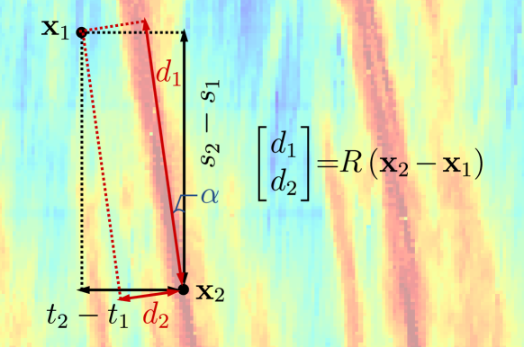
Figure 1: Illustration of the rotated coordinates.

A graphical illustration of our method is shown in Fig. 1. The intuition behind the proposed kernel is the rotation of the coordinates. The rotation angle $\alpha$ can be used to measure the speed of congestion propagation in the traffic wave. Similar to other hyper-parameters, the angle $\alpha$ can be estimated from the observed data.

III-D Model inference with variational sparse GP

The computational complexity of an MML estimation of GP scales cubically with the number of data points, which limits its applicability to large datasets. Therefore, we use the variational sparse GP (VSGP) [43] for scalable inference. VSGP introduces a set of $m$ inducing points at $Z=\left\{\mathbf{z}_{1},\cdots,\mathbf{z}_{m}\right\}$ that act as a sparse approximation to the full Gaussian process. The model assumes that the function values at the inducing points follow the same GP prior, and the posterior distribution of the function values is approximated by a Gaussian distribution conditioned on the inducing variables. The locations of inducing points can be optimized as other hyper-parameters.

The model parameters, including hyper-parameters $\bm{\theta}$ and the locations of inducing variables $Z$, are learned by maximizing the evidence lower bound (ELBO), which is a lower bound of the log marginal likelihood of the observed data. The ELBO of VSGP derived by Titsias [43] is:

$$\log p(\mathbf{y}_{o})\geq\log\mathcal{N}\left(\mathbf{y}_{o}|\mathbf{0},Q_{nn}+\sigma_{\varepsilon}^{2}I\right)-\frac{1}{2\sigma_{\varepsilon}^{2}}\operatorname{tr}\left(K_{nn}-Q_{nn}\right),$$ (13)

where $Q_{nn}=K_{nm}K_{mm}^{-1}K_{nm}^{\top}$, matrices $K_{mm}$ and $K_{nm}$ are the kernel evaluated at the inducing points, and between the observed locations and inducing points, respectively. We can interpret the ELBO as the sum of the approximate log marginal likelihood and a regularization term $-\frac{1}{2\sigma_{\varepsilon}^{2}}\operatorname{tr}\left(K_{nn}-Q_{nn}\right)$. The regularization term minimizes the squared error of predicting the training latent function values $\mathbf{f}_{n}$ from the inducing variables. Eq. (13) can be simplified with the Woodbury matrix identity, and the time complexity of VSGP is $O(mn^{2})$.

The posterior distribution of function values at unknown location $\mathbf{x}_{*}$ is given by the integral $p(\mathbf{f}_{*})=\int p(\mathbf{f}_{*}|\mathbf{f}_{z})p(\mathbf{f}_{z})d\mathbf{f}_{z}$, which is a Gaussian distribution with the mean and covariance:

$$\bar{\mathbf{f}}_{*} =K_{*m}K_{mm}^{-1}\bar{\mathbf{f}}_{z},$$ (14)

$$\operatorname{cov}(\mathbf{f}_{*}) =K_{**}-K_{m*}^{\top}K_{mm}^{-1}K_{m*}+K_{m*}^{\top}K_{mm}^{-1}\Lambda K_{mm}^{-1}K_{m*},$$ (15)

where $\bar{\mathbf{f}}_{z}=\sigma_{\varepsilon}^{-2}\Lambda^{-1}K_{mm}^{-1}K_{mn}\mathbf{y}_{o}$ is the posterior mean of the inducing variables, and $\Lambda=K_{mm}^{-1}+\sigma_{\varepsilon}^{-2}K_{mm}^{-1}K_{mn}K_{nm}K_{mm}^{-1}$ is the posterior precision matrix of the inducing variables.

III-E Multi-output GP

The TSE in a highway segment with multiple lanes can be naturally modeled using a multi-output GP model [44, 45], also known as a coregionalized GP or co-kriging. Unlike using independent GP models for each lane, a multi-output GP model can leverage the correlation between the traffic states of different lanes to improve estimation accuracy. In Section IV-F, we will demonstrate that the multi-output GP model can estimate traffic speed during a long period that has no observations in a lane, by utilizing information from the other lane.

The probe vehicles from different lanes locate at different spatiotemporal locations, which is referred to as heterotopic data in the multi-output GP literature. We model the traffic states of $L$ different lanes as a multi-output function $\bm{f}\left(\mathbf{x}\right)=\left[f^{1}(\mathbf{x}),\cdots,f^{L}(\mathbf{x})\right]^{\top}$ with a GP prior. The covariance of the $i$-th output at $\mathbf{x}$ and the $j$-th output at $\mathbf{x}^{\prime}$ is given by the kernel function:

$$k_{\operatorname{multi}}\left(f^{i}(\mathbf{x}),f^{j}(\mathbf{x}^{\prime})\right)=k(\mathbf{x},\mathbf{x}^{\prime})B\left[i,j\right],$$ (16)

where $B$ is an $L\times L$ symmetric and positive-definite matrix parametrized by $B=AA^{\top}$, and $A\in\mathbb{R}^{L\times r}$ is a parameter to learn, $r$ is the rank of $A$. This kernel parametrization is also called the intrinsic model of coregionalization [44] in the geostatistics literature. One can view the multi-output kernel $k_{\operatorname{multi}}$ as functions on an extended input space with the index of the lane, which allows for using the same inference procedure as the single-output GP model.

IV Case Study

In this section, we evaluate the proposed GP-based TSE method on two real-world datasets: the NGSIM [46] traffic trajectory data and the HighD [47] naturalistic vehicle trajectory data. Then, considering current and future mixed traffic of CVs and HVs, we compare TSE performance under different CV penetration rates and compare the proposed rotated GP method with other benchmark models, including adaptive smoothing interpolation method (ASM) [41], Spatiotemporal Hankel Low-Rank Tensor Completion (STH-LRTC) [6], and standard GP with ARD kernel. We also explore the use of multi-output rotated GP for TSE on multiple lanes.

IV-A Data and experimental setup

We test the proposed rotated GP TSE using the trajectories from two real-world datasets, namely NGSIM [46] and HighD [47]. Both datasets provide detailed information about each vehicle’s trajectory, such as vehicle ID, recording frame, time, location, velocity, lane, etc. This allows us to use the ground truth traffic state to evaluate the accuracy of TSE. In the case of NGSIM, we focus on the traffic data from lane 2 of US Highway 101. For HighD, we utilize data from two lanes of a German highway. The specific details of the two datasets are provided below:

• The NGSIM data: We use vehicle trajectories extracted from video cameras on lane 2 of US highway 101. In contrast to the previous work by Wang et al. [6], our experiment covers a longer road segment of 600 meters and a larger time range of 2500 seconds. We extract the complete data and focus on the traffic state at a $200\times 500$ spatiotemporal grid with a resolution of 3 meters and 5 seconds, where the traffic state is defined as the average vehicle speed in each grid cell. Fig. 2 (a) and (b) show the traffic speed maps of the entire dataset and samples of observed trajectories under a 5% penetration rate, respectively.

• The HighD data: This dataset provides naturalistic vehicle trajectories recorded on German highways using drones. The dataset includes 60 recordings from six different locations; each recording is identified by track ID. In our study, we focus on the recording with track ID 25. Where the full drive length of vehicles during the road segment is 1120346.1 meters, and the time range is 80676.08 seconds. To make the most of the data, we extract traffic state in a spatiotemporal grid of size $100\times 220$ with a resolution of 4 meters and 5 seconds, representing a domain of 400 meters and 1100 seconds. The average vehicle speed is calculated to describe the traffic state at each cell. We use the data from lane 4 for the TSE of a single lane in Table. II, and we use the data from lane 3 and lane 4 to test using multi-output GP for TSE.

For each dataset, we set 5%, 10%, 20%, 30%, 40%, and 50% as the penetration rate of CVs and assume only the trajectories of CVs are observed (i.e., the training data). Under each CV penetration rate, we repeat the experiment 10 times with different random draws of trajectories. Note that we define spatiotemporal grids to make an easy comparison with other models, although GP can make TSE on a continuous space without defining grids. Overall, the NGSIM and HighD datasets provide rich sources of data for evaluating the effectiveness and efficiency of our approach and baselines under different scenarios.

IV-B Baseline models and hyper-parameters

To compare the performance of the proposed GP based on rotated kernels (GP-rotated) with other methods, we use the following baselines:

• The adaptive smoothing interpolation method (ASM) [41]: It is an interpolation method for estimating smooth spatiotemporal traffic states. This method resembles the proposed rotated GP in terms of considering the traffic wave propagation using an anisotropic interpolation. We set the propagation speed of congestion to be -15km/h and the propagation speed of free traffic to be 70 km/h, which are adopted from the authors [41].

• Spatiotemporal Hankel Low-Rank Tensor Completion (STH-LRTC) [6]: It transforms the original speed matrix into a tensor using spatial and temporal delay embedding. Then, the approach estimated the traffic state matrix by conducting inverse Hankelization on the delay-embedding tensor imputed by a low-rank model. The key parameters include the embedding lengths $\tau_{s}$ and $\tau_{t}$. We adopt the same hyper-parameter settings $\tau_{s}=40$ and $\tau_{t}=30$ as the author. But we do find the method produces poor results in certain cases with extremely low CV penetration rates. Therefore, we increase the $\tau_{s}$ and $\tau_{t}$ with case-specific tuning, as noted in Table III.

• Gaussian process regression with standard ARD Matérn kernels (GP-ARD): It extends the basic GP by allowing the kernel function to have a separate length scale parameter for each input dimension, which enables the model to automatically determine the importance of each input variable in predicting the output variable. The hyper-parameters are learned from data using the VSGP approach.

In the following, we refer to the proposed method “GP-rotated”. And we use Matérn kernel [8] as the basic kernel function for all GP models. We set the number of inducing points $m=\min\left(0.02n,500\right)$, and the initial locations of inducing points are randomly distributed on the grid. As introduced in Section III-D, the hyper-parameters of GP-rotated can be learned from the observed data, which could be time-consuming for a large dataset. However, one may not need to repeatedly learn the hyper-parameters for the same highway segment in reality. Therefore, we also test the performance of the proposed GP using pre-trained hyper-parameters, referred to as “P-GP-rotated”.

We perform TSE only for the cells without any CV trajectories. For cells with observed trajectories, we directly use the speed from the training data. It’s worth noting that the training data (obtained from CVs) and test data (obtained from all vehicles) for a cell with CV trajectories may differ since the speed may be calculated from different numbers of vehicles in the training and test data. Finally, we use the root mean squared error (RMSE) and mean absolute error (MAE) as shown in the following to evaluate the performance of different TSE models:

RMSE $$=\sqrt{\frac{\sum_{l}\sum_{s}\sum_{t}(y^{l}(s,t)-\hat{y}^{l}(s,t))^{2}}{STL}},$$ (17)

MAE $$=\frac{\sum_{l}\sum_{s}\sum_{t}|y^{l}(s,t)-\hat{y}^{l}(s,t)|}{STL}.$$ (18)

IV-C Performance evaluation: NGSIM and HighD

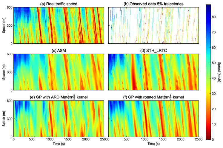
Figure 2: An TSE experiment on the NGSIM dataset with 5% CVs penetration rate. The observed trajectories are superimposed on the TSE results. (a) The traffic speed of the full dataset. (b) The traffic speed of observed trajectories. (c) The traffic speed estimated by the ASM method. (d) The traffic speed estimated by the STH-LRTC method. (e) The traffic speed estimated by the GP with ARD Matérn$\frac{5}{2}$ kernel. (f) The traffic speed estimated by the GP with the proposed rotated Matérn$\frac{5}{2}$ kernel.

We begin by visually examining the TSE performance of different methods under a 5% CV penetration rate using the NGSIM dataset. Figure 2 displays the results. Figure 2 (a) shows the ground truth traffic speed map of all trajectories, exhibiting complex traffic dynamics evolution with shock waves, making it a suitable dataset for experimentation. Figure 2 (b) displays one of the randomly selected 5% training datasets from ten independent experiments.

By comparing Fig. 2 (e) and (f). We can observe that the proposed GP-rotated captures the directional traffic speed correlations that traditional GP-ARD cannot model. When comparing the ASM in Fig. 2 (c) with the proposed GP-rotated, we can find they both capture the congestion propagation in the traffic wave because they both use the idea of anisotropic kernels. However, the congestion speed estimated by the ASM is generally lower than the ground truth speed, which is caused by the “smoothing” operation in the ASM. The STH-LRTC in Fig. 2 (d) also captures the congestion propagation in the traffic wave, but it performs poorly when there is a long period without CV trajectories (e.g., 550s-750s).

Next, we perform more extensive experiments to quantify the performance of the proposed method and the baselines under different penetration rates. For each penetration rate (percentage of trajectories). For each penetration rate (5%, 10%, 20%, 30%, 40%, and 50%), we repeat the experiments ten times with randomly selected vehicle trajectories from the complete dataset as the training set (see Section IV-A). The experiments were conducted on the NGSIM and HighD datasets. Table I and Table II display the average MAE (m/s) and RMSE (m/s) with standard deviation for each method under various penetration rates and datasets.

TABLE I: Performance of the proposed method and baselines under different penetration rates. (NGSIM), mean (std).

Method	ASM		STH-LRTC		GP-ARD		GP-rotated		P-GP-rotated
Rate	MAE	RMSE	MAE	RMSE	MAE	RMSE	MAE	RMSE	MAE	RMSE
0.05	5.59(0.36)	7.81(0.56)	5.51(1.36)	7.94(2.38)	6.02(0.36)	8.62(0.56)	4.85(0.31)	6.74(0.56)	4.97(0.29)	6.74(0.47)
0.1	4.42(0.17)	6.28(0.27)	4.19(1.39)	7.43(5.62)	4.35(0.30)	6.42(0.58)	3.82(0.22)	5.44(0.47)	3.79(0.13)	5.19(0.22)
0.2	3.53(0.10)	5.31(0.14)	3.01(1.26)	6.16(7.14)	3.07(0.14)	4.61(0.26)	2.81(0.10)	4.10(0.19)	2.98(0.08)	4.28(0.12)
0.3	2.93(0.06)	4.69(0.10)	2.09(0.05)	3.17(0.12)	2.43(0.06)	3.77(0.11)	2.27(0.05)	3.43(0.10)	2.48(0.05)	3.75(0.08)
0.4	2.44(0.06)	4.21(0.10)	1.75(0.05)	2.81(0.12)	2.03(0.06)	3.35(0.11)	1.92(0.05)	3.08(0.09)	2.09(0.05)	3.37(0.09)
0.5	1.99(0.06)	3.75(0.09)	1.43(0.04)	2.46(0.11)	1.67(0.04)	2.96(0.10)	1.58(0.04)	2.71(0.09)	1.71(0.04)	2.98(0.07)

TABLE II: Performance of the proposed method and baselines under different penetration rates. (HighD), mean (std).

Method	ASM		STH-LRTC		GP-ARD		GP-rotated		P-GP-rotated
Rate	MAE	RMSE	MAE	RMSE	MAE	RMSE	MAE	RMSE	MAE	RMSE
0.05	5.58(0.37)	6.37(0.63)	55.9(29.3)	121.5(51.1)	5.18(1.59)	7.19(2.04)	4.48(0.50)	6.27(0.94)	4.43(0.27)	6.06(0.43)
0.1	3.39(0.13)	4.81(0.18)	3.19(0.10)	4.49(0.21)	3.22(0.17)	4.55(0.28)	3.18(0.16)	4.45(0.25)	3.55(0.18)	5.00(0.30)
0.2	2.61(0.08)	3.91(0.13)	2.15(0.11)	3.12(0.18)	2.23(0.09)	3.26(0.15)	2.23(0.09)	3.25(0.13)	2.43(0.07)	3.52(0.11)
0.3	2.13(0.03)	3.41(0.05)	1.65(0.04)	2.49(0.06)	1.71(0.05)	2.62(0.10)	1.71(0.05)	2.61(0.10)	1.89(0.05)	2.90(0.09)
0.4	1.72(0.04)	2.95(0.07)	1.31(0.04)	2.07(0.07)	1.36(0.04)	2.14(0.09)	1.35(0.03)	2.14(0.08)	1.49(0.03)	2.39(0.06)
0.5	1.40(0.05)	2.59(0.10)	1.05(0.03)	1.75(0.07)	1.09(0.03)	1.80(0.07)	1.09(0.03)	1.80(0.06)	1.19(0.03)	2.03(0.05)

Table I and Table II illustrate that the performance of the STH-LRTC method is the best when the proportion of observed trajectories (penetration rate) is over 30%. This is because the GP-based methods cannot capture the fine-grained texture in traffic flow, which is shown in Section IV-D. However, for the cases with sparse observations (CV penetration from 5% to around 20%), our proposed GP-rotated performs the best on both NGSIM and HighD datasets. As the decrease of CV penetration rate, the STH-LRTC may fail due to a large block of missing information, which can be observed in the HighD data under the 5% rate. The corresponding MAE and RMSE values can be as high as 55.9 m/s and 121.5 m/s, respectively. The STH-LRTC may be unstable under low penetration rates, with high standard deviation in MAE and RMSE values. In contrast, our proposed GP method provides a very robust estimation, regardless of the percentage of probe vehicles. In the early stages of a mixed traffic environment with a low CV penetration rate, such as 5% to 20%, our proposed method is a suitable choice.

Our proposed method consistently outperforms the ASM benchmark. An advantage of ASM is that it considers the traffic propagation of both congestion flow and free flow. Therefore, ASM could produce a more natural traffic flow pattern, as demonstrated in high-speed region (top left corner) of in Fig. 2 (c). However, the ASM struggles to impute small shock waves during the first 500 seconds (bottom left corner). Our proposed GP methods, on the other hand, consistently demonstrate superior performance compared to ASM, regardless of the penetration rate. The average gaps in MAE (m/s) and RMSE (m/s) between ASM and GP-rotated are around 0.3-0.9 m/s, highlighting the superiority of our approach.

We also compare the GP-ARD and GP-rotated methods using the Matérn$\frac{5}{2}$ kernel in Tables I and II. Our results show that the GP-rotated method consistently outperforms the GP-ARD method in terms of average MAE and RMSE, regardless of whether we use the pre-trained parameters or not. This can be attributed to the fact that the ARD kernel is isotropic, meaning it uses distance to measure covariance. However, traffic waves are anisotropic and propagate in spatiotemporal directions. Although GP-ARD can apply different length scales to different dimensions, it still fails to capture the directional covariance of traffic waves. On the other hand, our proposed anisotropic GP-rotated method with a directional hyper-parameter $alpha$ accurately models the directional covariance of traffic waves. Furthermore, we observed that the numerical differences in MAE and RMSE between GP-ARD and GP-rotated decrease with an increase in the observation rate. This is because, with more observed trajectories, the GP-ARD method can utilize more information to overcome the directional limitation based on length scale adjustments.

Finally, we observe that the P-GP-rotated method can also achieve satisfactory TSE results and even outperform the GP-rotated in some low-penetration scenarios, possibly due to the overfitting of GP-rotated when the number of observed trajectories is small. However, as the CV penetration rate increases, the performance of P-GP-rotated is not as good as GP-rotated, likely because the inducing point locations in P-GP-rotated are not optimized. The proposed GP kernel hyperparameters, $\alpha$, represent the angle between the traffic wave and the spatial direction, and values learned from the data are around $\alpha=0.108=6.20^{\circ}$ for the NGSIM dataset and $\alpha=0.160=9.16^{\circ}$ for the HighD dataset. After unit conversion with the size of cells, our estimation shows that the congestion propagation speed is approximately -19.87 km/h and -17.86 km/h for the NGSIM and HighD datasets, respectively, which is faster than the -15 km/h value used in Treiber et al. [41].

IV-D Uncertainty quantification

Our research incorporates uncertainty quantification as a crucial aspect to enable reliable and accurate predictions while acknowledging the inherent variability and unpredictability of the system under investigation, which is a lacking feature in existing methods. The GP framework provides a natural way to quantify uncertainty through the predictive covariance matrix, as shown in Eq. (15). We can use the diagonal elements of the covariance matrix (i.e., variance) to quantify the uncertainty of the TSE at each cell. The comparison between the TSE residuals and the uncertainty is presented in Fig. 3, which provides a comprehensive understanding of the uncertainties associated with our findings.

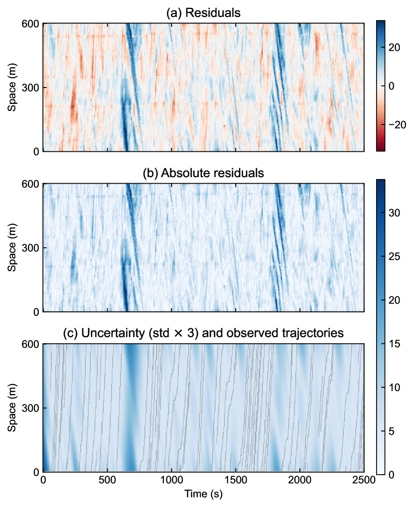
Figure 3: The uncertainty quantification of the GP-rotated estimation method on the NGSIM dataset with 5% observed trajectories. (a) The residuals of the estimation. (b) The absolute residuals of the estimation. (c) The uncertainty and 5% observed trajectories.

The uncertainties (shown by three standard deviations) of the TSE using GP-rotated and the observed trajectories are demonstrated in Fig. 3 (c). First, we can find that the uncertainties are larger for regions with no CV trajectories, such as time ranges of 600 s to 700 s and 1800 s to 1900 s. It is notable that the uncertainty is anisotropic, propagating along the traffic wave, highlighting the need for an approach that can accurately capture this behavior. By comparing Fig. 3 (b) and (c), we can find that the predictive uncertainties are, in general, consistent with the absolute residuals, meaning the predictive variance of GP-rotated is a reliable indicator for uncertainty quantification.

Finally, if we look at Fig. 3 (a), we can find that there are still spatiotemporal correlations in the residuals, meaning that there is still space for improvement in the TSE estimation. For example, we can use the addition of multiple GP kernels, one for the congestion propagation and the other for the free-flow traffic, to capture the complex traffic dynamics. We have accurately tried to use the multiple GP kernels in our research, but the results do not improve. We believe that the reason is that the propagation of free flow speed is not as apparent as the congestion propagation, which does not provide enough information to improve the TSE estimation. But the correlations in the residuals still indicate that a more capable kernel design is needed to capture the complex traffic dynamics.

In conclusion, our research emphasizes the importance of using an approach that can accurately capture the behavior of traffic waves in TSE. The GP-rotated method we propose is crucial in accounting for uncertainty propagation and allows us to provide reliable and accurate predictions. Through our approach, we can evaluate the validity of our model while also providing a measure of confidence in our predictions.

IV-E Computational time

In Table III, we present the running time taken by four different methods, namely ASM, STH-LRTC, GP-rotated, and Pre-trained GP-rotated (P-GP-rotated), on both NGSIM and HighD datasets. Among these methods, the P-GP-rotated approach stands out for its significant shorter computational time. This is because the P-GP-rotated method uses fixed kernel hyperparameters and random inducing points without any learning process. It is worth noting that ASM and STH-LRTC also use fixed parameters without any optimization, which makes it appropriate to compare them with P-GP-rotated rather than GP-rotated.

We can see the running time in the highD dataset is faster than the NGSIM dataset. This is because the highD dataset has a smaller grid size. The computational time of STH-LRTC is considerably higher compared to other methods. For instance, on HighD data, it takes approximately 20 to 60 times longer than the P-GP-rotated method and 15 to 30 times longer than ASM computation. Moreover, the computational efficiency of STH-LRTC drops significantly when the penetration rate is 0.05 and 0.1. This is mainly due to the increase in the spatiotemporal delay embedding lengths ($\tau_{s}$ and $\tau_{t}$), which impacts the computation time substantially. As a result, the computational cost of STH-LRTC becomes extremely high under such scenarios.

We observe that the computational time of ASM, GP-rotated, and P-GP-rotated methods increases as the observation rate increases. This is understandable as more data needs to be processed, leading to higher computation costs due to the increased traffic information. On the other hand, we noticed that the computational time of STH-LRTC decreases as the observation rate increases. This could be because STH-LRTC benefits from the increased amount of observed data, resulting in fewer delay-embedding and interaction steps. However, it is essential to note that this trend might not always hold, and a slight change in the parameters of the delay embedding in STH-LRTC could alter the trend.

TABLE III: Computational time in seconds, mean (std).

NGSIM
Rate	ASM	STH-LRTC	GP-rotated	P-GP-rotated
0.05	7.40 (0.57)	908.21 (38.61)a	27.30 (2.92)	3.84 (0.27)
0.1	14.18 (0.43)	850.90 (19.61)a	77.54 (4.68)	9.25 (0.42)
0.2	26.77 (0.92)	206.72 (1.85)	153.07 (3.67)	13.43 (1.68)
0.3	38.38 (1.38)	199.99 (1.77)	204.61 (2.71)	13.97 (0.19)
0.4	48.15 (3.98)	196.09 (2.66)	245.37 (3.76)	14.94 (0.16)
0.5	54.21 (2.83)	191.46 (1.93)	280.01 (5.28)	15.85 (0.26)
HighD
Rate	ASM	STH-LRTC	GP-rotated	P-GP-rotated
0.05	0.46 (0.03)	67.61 (3.38)	11.97 (1.89)	0.35 (0.05)
0.1	0.87 (0.04)	823.65 (10.74)b	12.54 (0.29)	0.42 (0.05)
0.2	1.67 (0.07)	54.29 (1.39)	19.86 (0.40)	0.83 (0.16)
0.3	2.30 (0.05)	51.46 (1.06)	29.78 (0.66)	1.25 (0.15)
0.4	2.84 (0.08)	49.50 (0.89)	40.46 (0.86)	1.63 (0.21)
0.5	3.22 (0.09)	48.14 (0.82)	50.93 (1.49)	2.27 (0.21)

• Delay-embedding lengths $\tau_{s}=50$, $\tau_{t}=50$.

• Delay-embedding lengths $\tau_{s}=60$, $\tau_{t}=50$.

IV-F TSE in multiple lanes

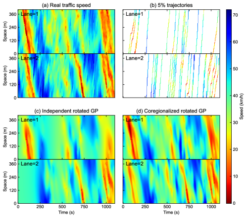
Figure 4: The TSE in multiple lanes on the HighD dataset. (a) The traffic speed profile of the full dataset. (b) The traffic speed profile of the 5% observed trajectories. (c) The traffic state is estimated by the independent rotated GP method. (d) The traffic state is estimated by the coregionalized rotated GP method.

TSE has been an active research area for many years, with many methods proposed for estimating the traffic state on an individual lane. Although some previous works have considered multi-lane TSE, most focus on modeling each lane independently without considering the correlations and interactions between neighboring lanes. This section demonstrates that we propose a novel approach to enhance the TSE by jointly modeling the traffic states on multiple lanes using the multi-output GP. Specifically, we use the trajectories from all lanes as the input features to the multi-output GP model and predict the traffic state for each lane as a separate output dimension. By sharing the same covariance structure across all output dimensions, the multi-output GP model can capture the correlations and dependencies between the traffic states on different lanes, leading to more accurate and robust predictions.

The correlation between traffic speed profiles on different lanes of a highway segment is evident from Fig. 4 (a). The ground truth traffic speed profiles for Lane 1 and Lane 2 demonstrate that these two lanes are correlated, with both lanes experiencing congestion during the first 200 seconds and the last 100 seconds of the observed period. From 250 s to 350 s, the traffic speeds on both lanes are high. However, when we have only 5% of trajectory data for each lane, accurately and simultaneously estimating the traffic state on these two lanes becomes challenging.

In Figure 4 (b), it can be observed that either Lane 1 or Lane 2 has a gap without any observations, lasting from 260 s to 490 s on lane 1 and from 0 to 250 s on lane 2, respectively. When using the independent GP-rotated method to perform TSE, the resulting traffic state profiles are shown in Figure 4 (c). It is evident from the figure that the speed map of Lane 1 does not contain much traffic information during the time period between 250 s and 500 s, while the speed map of Lane 2 loses most of the traffic information between 0 s and 250 s. These results demonstrate that performing independent TSE in each lane cannot achieve high estimation accuracy.

Despite the long periods of missing observations in either Lane 1 or Lane 2, we can observe that the trajectories from the other lane can compensate for the missing period, which is the main idea behind using a multi-output GP to output TSE in multiple lanes. Figure 4 (d) shows that the multi-output GP performs better than the independent GP method. The estimated traffic state profiles are almost identical to the original traffic speed maps. Specifically, during the period between 0 s and 250 s, the multi-output GP can reconstruct the shock wave of Lane 2 using the information from Lane 1, whereas the independent rotated GP fails to rebuild this shock wave, as demonstrated in Figure 4 (c) and (d).

V Conclusion and Discussion

This paper presents a novel approach for traffic speed estimation using Gaussian process regression with a rotated kernel parametrization. The rotated kernel is designed to model anisotropic traffic flow, allowing for capturing the directional dependence of traffic wave propagation. The proposed method is a generalization of the ARD kernel function and can be applied to other kernel functions like Matérn and rational quadratic kernels. To validate the effectiveness of the proposed method, we conduct experiments on two real-world datasets from the NGSIM and HighD programs. The results show that the proposed method outperforms other state-of-the-art methods in terms of both estimation accuracy, robustness, and computational efficiency. The proposed method can accurately capture the direction of traffic wave propagation, which cannot be achieved by traditional GP models with ARD kernels or other baselines. The proposed method also provides statistical uncertainty quantification, which is crucial for data-driven TSE models, especially under limited training data. We also extend the proposed method to conduct the TSE on multiple lanes simultaneously, not limited to just one lane. Overall, the proposed method is a promising approach for traffic speed estimation, offering improved performance and the ability to capture directional traffic flow patterns.

While the proposed method shows promising results in traffic speed estimation, there are some limitations and potential future research directions. First, the current model is only tested on the traffic speed estimation problem, and it may be possible to estimate speed, density, and other traffic state variables simultaneously using multi-output Gaussian process regression. Second, future research can extend the model to assess the traffic wave by incorporating additional information, such as traffic signals and road geometry, to make the model suitable for more scenarios. Third, the proposed method is evaluated on real-world trajectory datasets that simulate the trajectory data obtained from connected vehicles. To further validate the effectiveness of the proposed method, it is suggested to test on commercial CV datasets.

Fan Wu (Student Member, IEEE) received a B.S. degree in Traffic Engineering from Southeast University, Nanjing, China, in 2017, and an M.S. degree in Communication and Transportation Engineering from Harbin Institute of Technology, Harbin, China, in 2019. She is currently working toward a Ph.D. degree in the Department of Civil and Environmental Engineering at the University of Alberta, Edmonton, AB, Canada. Her research interests include intelligent transportation systems, traffic control and operation for connected autonomous vehicles.

Zhanhong Cheng (Member, IEEE) received the B.S. and M.S. degrees from the Harbin Institute of Technology, Harbin, China, and the Ph.D. degree from McGill University, Montreal, QC, Canada, where he is currently a Postdoctoral Researcher with the Department of Civil Engineering. His research interests include public transportation, travel behavior modeling, spatiotemporal forecasting, and machine learning in transportation.

Huiyu Chen received the B.Eng. degree (Yisheng Mao hons.) in transportation engineering from Southwest Jiaotong University, Chengdu, China, in 2015 and M.Sc. degree in transportation engineering from Tongji University, Shanghai, China, in 2018. She is currently working toward the Ph.D. degree in the Department of Civil and Environmental Engineering, University of Alberta, Edmonton, AB, Canada. Her research interests include network modeling and intelligent traffic operation and control for connected and autonomous vehicles.

Tony Z. Qiu is a Professor in the Department of Civil and Environmental Engineering at the University of Alberta (U of A) and holds both the Canada Research Chair in Cooperative Transportation Systems and the NSERC Industrial Research Chair in Intelligent Transportation Systems. Since joining the U of A in 2009, Dr. Qiu founded the Intelligent Transportation Systems (ITS) research lab, now called the Centre for Smart Transportation (CST). He is also the Scientific Director for the Autonomous Systems Initiative (ASI), a multi-million dollar Campus Alberta research program focused on developing Artificial Intelligence and automated systems. Dr. Qiu received his Ph.D. from the University of Wisconsin-Madison in 2007 and his BSc. and MSc. from Tsinghua University of China in 2001 and 2003, respectively. From 2008-2009, he worked as a postdoctoral researcher in the California PATH Program at the University of California, Berkeley. His research focuses on developing analytical models to evaluate and optimize large and complex ITS networks and develop support tools for the agencies that manage these systems. In addition to having completed over 41 research projects totalling more than $6,000,000 in funding, he has published over 160 journal and conference papers, several of which have been chosen for best paper awards. He has also received the 2013 Minister’s Award of Excellence in Process Innovation, the 2015 Faculty of Engineering Research Award from the University of Alberta, an award at the 2016 ITS Canada Annual Conference for research collaboration with the City of Edmonton and was recently named the Young ITS Canada Leadership award for contributions to the advancement of Intelligent Transportation Systems (June 2019). Through his leadership of the CST, Dr. Qiu is working to foster Canadian competitiveness in Connected Vehicle (CV) technology and research by developing Canada’s first CV testbed, ACTIVE-AURORA, a network of six on-road and in-lab test beds equipped and linked with CV technology. ACTIVE-AURORA provides an ITS and CV testing ground and a multi-institutional collaboration platform.

Lijun Sun (Senior Member, IEEE) received the B.S. degree in civil engineering from Tsinghua University, Beijing, China, in 2011, and a Ph.D. degree in civil engineering (transportation) from the National University of Singapore in 2015. He is currently an Assistant Professor with the Department of Civil Engineering and a William Dawson Scholar at McGill University, Montreal, QC, Canada. His research centers on intelligent transportation systems, machine learning, spatiotemporal modeling, travel behavior, and agent-based simulation.

References

- Seo et al. [2017] T. Seo, A. M. Bayen, T. Kusakabe, and Y. Asakura, “Traffic state estimation on highway: A comprehensive survey,” Annual reviews in control, vol. 43, pp. 128–151, 2017.
- Lighthill and Whitham [1955] M. J. Lighthill and G. B. Whitham, “On kinematic waves ii. a theory of traffic flow on long crowded roads,” Proceedings of the Royal Society of London. Series A. Mathematical and Physical Sciences, vol. 229, no. 1178, pp. 317–345, 1955.
- Richards [1956] P. I. Richards, “Shock waves on the highway,” Operations research, vol. 4, no. 1, pp. 42–51, 1956.
- Payne [1971] H. J. Payne, “Model of freeway traffic and control,” Mathematical Model of Public System, pp. 51–61, 1971.
- Whitham [2011] G. B. Whitham, Linear and nonlinear waves. John Wiley & Sons, 2011.
- Wang et al. [2021] X. Wang, Y. Wu, D. Zhuang, and L. Sun, “Low-rank hankel tensor completion for traffic speed estimation,” arXiv preprint arXiv:2105.11335, 2021.
- Thodi et al. [2022] B. T. Thodi, Z. S. Khan, S. E. Jabari, and M. Menéndez, “Incorporating kinematic wave theory into a deep learning method for high-resolution traffic speed estimation,” IEEE Transactions on Intelligent Transportation Systems, 2022.
- Rasmussen et al. [2006] C. E. Rasmussen, C. K. Williams et al., Gaussian processes for machine learning. Springer, 2006, vol. 1.
- Aw and Rascle [2000] A. Aw and M. Rascle, “Resurrection of” second order” models of traffic flow,” SIAM journal on applied mathematics, vol. 60, no. 3, pp. 916–938, 2000.
- Zhang [2002] H. M. Zhang, “A non-equilibrium traffic model devoid of gas-like behavior,” Transportation Research Part B: Methodological, vol. 36, no. 3, pp. 275–290, 2002.
- Vishnoi et al. [2022] S. C. Vishnoi, S. A. Nugroho, A. F. Taha, and C. G. Claudel, “Traffic state estimation for connected vehicles using the second-order aw-rascle-zhang traffic model,” arXiv preprint arXiv:2209.02848, 2022.
- Nanthawichit et al. [2003] C. Nanthawichit, T. Nakatsuji, and H. Suzuki, “Application of probe-vehicle data for real-time traffic-state estimation and short-term travel-time prediction on a freeway,” Transportation research record, vol. 1855, no. 1, pp. 49–59, 2003.
- Mihaylova et al. [2006] L. Mihaylova, R. Boel, and A. Hegyi, “An unscented kalman filter for freeway traffic estimation,” IFAC Proceedings Volumes, vol. 39, no. 12, pp. 31–36, 2006.
- Wang and Papageorgiou [2005] Y. Wang and M. Papageorgiou, “Real-time freeway traffic state estimation based on extended kalman filter: a general approach,” Transportation Research Part B: Methodological, vol. 39, no. 2, pp. 141–167, 2005.
- Work et al. [2010] D. B. Work, S. Blandin, O.-P. Tossavainen, B. Piccoli, and A. M. Bayen, “A traffic model for velocity data assimilation,” Applied Mathematics Research eXpress, vol. 2010, no. 1, pp. 1–35, 2010.
- Van Hinsbergen et al. [2011] C. P. Van Hinsbergen, T. Schreiter, F. S. Zuurbier, J. Van Lint, and H. J. Van Zuylen, “Localized extended kalman filter for scalable real-time traffic state estimation,” IEEE transactions on intelligent transportation systems, vol. 13, no. 1, pp. 385–394, 2011.
- Makridis and Kouvelas [2023] M. A. Makridis and A. Kouvelas, “An adaptive framework for real-time freeway traffic estimation in the presence of cavs,” Transportation Research Part C: Emerging Technologies, vol. 149, p. 104066, 2023.
- Mihaylova et al. [2007] L. Mihaylova, R. Boel, and A. Hegyi, “Freeway traffic estimation within particle filtering framework,” Automatica, vol. 43, no. 2, pp. 290–300, 2007.
- Treiber and Helbing [2002] M. Treiber and D. Helbing, “Reconstructing the spatio-temporal traffic dynamics from stationary detector data,” Cooperative Transportation Dynamics, vol. 1, no. 3, pp. 3–1, 2002.
- Zhong et al. [2004] M. Zhong, P. Lingras, and S. Sharma, “Estimation of missing traffic counts using factor, genetic, neural, and regression techniques,” Transportation Research Part C: Emerging Technologies, vol. 12, no. 2, pp. 139–166, 2004.
- Ni and Leonard [2005] D. Ni and J. D. Leonard, “Markov chain monte carlo multiple imputation using bayesian networks for incomplete intelligent transportation systems data,” Transportation research record, vol. 1935, no. 1, pp. 57–67, 2005.
- Yin et al. [2012] W. Yin, P. Murray-Tuite, and H. Rakha, “Imputing erroneous data of single-station loop detectors for nonincident conditions: Comparison between temporal and spatial methods,” Journal of Intelligent Transportation Systems, vol. 16, no. 3, pp. 159–176, 2012.
- Tak et al. [2016] S. Tak, S. Woo, and H. Yeo, “Data-driven imputation method for traffic data in sectional units of road links,” IEEE Transactions on Intelligent Transportation Systems, vol. 17, no. 6, pp. 1762–1771, 2016.
- Jia et al. [2016] Y. Jia, J. Wu, and Y. Du, “Traffic speed prediction using deep learning method,” in 2016 IEEE 19th international conference on intelligent transportation systems (ITSC). IEEE, 2016, pp. 1217–1222.
- Rempe et al. [2022] F. Rempe, P. Franeck, and K. Bogenberger, “On the estimation of traffic speeds with deep convolutional neural networks given probe data,” Transportation research part C: emerging technologies, vol. 134, p. 103448, 2022.
- Han and Ahn [2021] Y. Han and S. Ahn, “Estimation of traffic flow rate with data from connected-automated vehicles using bayesian inference and deep learning,” Frontiers in Future Transportation, vol. 2, p. 644988, 2021.
- Shi et al. [2021a] R. Shi, Z. Mo, K. Huang, X. Di, and Q. Du, “A physics-informed deep learning paradigm for traffic state and fundamental diagram estimation,” IEEE Transactions on Intelligent Transportation Systems, vol. 23, no. 8, pp. 11 688–11 698, 2021.
- Shi et al. [2021b] R. Shi, Z. Mo, and X. Di, “Physics-informed deep learning for traffic state estimation: A hybrid paradigm informed by second-order traffic models,” in Proceedings of the AAAI Conference on Artificial Intelligence, vol. 35, no. 1, 2021, pp. 540–547.
- Xu et al. [2020] D. Xu, C. Wei, P. Peng, Q. Xuan, and H. Guo, “Ge-gan: A novel deep learning framework for road traffic state estimation,” Transportation Research Part C: Emerging Technologies, vol. 117, p. 102635, 2020.
- Li et al. [2013] L. Li, Y. Li, and Z. Li, “Efficient missing data imputing for traffic flow by considering temporal and spatial dependence,” Transportation research part C: emerging technologies, vol. 34, pp. 108–120, 2013.
- Seo et al. [2015a] T. Seo, T. Kusakabe, and Y. Asakura, “Traffic state estimation with the advanced probe vehicles using data assimilation,” in 2015 IEEE 18th International Conference on Intelligent Transportation Systems. IEEE, 2015, pp. 824–830.
- Florin and Olariu [2016] R. Florin and S. Olariu, “On a variant of the mobile observer method,” IEEE Transactions on Intelligent Transportation Systems, vol. 18, no. 2, pp. 441–449, 2016.
- Seo and Kusakabe [2015] T. Seo and T. Kusakabe, “Probe vehicle-based traffic state estimation method with spacing information and conservation law,” Transportation Research Part C: Emerging Technologies, vol. 59, pp. 391–403, 2015.
- Yuan et al. [2014] Y. Yuan, H. Van Lint, F. Van Wageningen-Kessels, and S. Hoogendoorn, “Network-wide traffic state estimation using loop detector and floating car data,” Journal of Intelligent Transportation Systems, vol. 18, no. 1, pp. 41–50, 2014.
- Seo et al. [2015b] T. Seo, T. Kusakabe, and Y. Asakura, “Estimation of flow and density using probe vehicles with spacing measurement equipment,” Transportation Research Part C: Emerging Technologies, vol. 53, pp. 134–150, 2015.
- Kyriacou et al. [2022] V. Kyriacou, Y. Englezou, C. G. Panayiotou, and S. Timotheou, “Bayesian traffic state estimation using extended floating car data,” IEEE Transactions on Intelligent Transportation Systems, 2022.
- Usama et al. [2022] M. Usama, R. Ma, J. Hart, and M. Wojcik, “Physics-informed neural networks (pinns)-based traffic state estimation: An application to traffic network,” Algorithms, vol. 15, no. 12, p. 447, 2022.
- Chen and Levin [2019] R. Chen and M. W. Levin, “Traffic state estimation based on kalman filter technique using connected vehicle v2v basic safety messages,” in 2019 IEEE Intelligent Transportation Systems Conference (ITSC). IEEE, 2019, pp. 4380–4385.
- Fountoulakis et al. [2017] M. Fountoulakis, N. Bekiaris-Liberis, C. Roncoli, I. Papamichail, and M. Papageorgiou, “Highway traffic state estimation with mixed connected and conventional vehicles: Microscopic simulation-based testing,” Transportation Research Part C: Emerging Technologies, vol. 78, pp. 13–33, 2017.
- Bekiaris-Liberis et al. [2017] N. Bekiaris-Liberis, C. Roncoli, and M. Papageorgiou, “Highway traffic state estimation per lane in the presence of connected vehicles,” Transportation research part B: methodological, vol. 106, pp. 1–28, 2017.
- Treiber et al. [2011] M. Treiber, A. Kesting, and R. E. Wilson, “Reconstructing the traffic state by fusion of heterogeneous data,” Computer-Aided Civil and Infrastructure Engineering, vol. 26, no. 6, pp. 408–419, 2011.
- NEAL [1996] R. NEAL, “Bayesian learning for neural networks,” Lecture Notes in Statistics, 1996.
- Titsias [2009] M. Titsias, “Variational learning of inducing variables in sparse gaussian processes,” in Artificial intelligence and statistics. PMLR, 2009, pp. 567–574.
- Wackernagel [2003] H. Wackernagel, Multivariate geostatistics: an introduction with applications. Springer Science & Business Media, 2003.
- Bonilla et al. [2007] E. V. Bonilla, K. Chai, and C. Williams, “Multi-task gaussian process prediction,” Advances in neural information processing systems, vol. 20, 2007.
- NGSIM [2007] NGSIM, “Us highway 101 dataset,” 2007. [Online]. Available: https://www.fhwa.dot.gov/publications/research/operations/07030/index.cfm
- Krajewski et al. [2018] R. Krajewski, J. Bock, L. Kloeker, and L. Eckstein, “The highd dataset: A drone dataset of naturalistic vehicle trajectories on german highways for validation of highly automated driving systems,” in 2018 21st International Conference on Intelligent Transportation Systems (ITSC), 2018, pp. 2118–2125.