Quantum Steganography via Coherent and Fock State Encoding in an Optical Medium
Abstract
Steganography is an alternative to cryptography, where information is protected by secrecy—being disguised as innocent communication or noise—rather than being scrambled. In this work we develop schemes for steganographic communication using Fock and coherent states in optical channels based on disguising the communications as thermal noise, with a fidelity approaching 1. We derive bounds on their efficiency in terms of the communication rate and the required keyrate in the case of an all-powerful eavesdropper, and provide explicit methods of encoding and error correction for the noiseless channel case.
I Introduction
Covert communication is often associated with military or espionage applications, but some of the earliest applications were for personal use. In Ancient Egypt, hieroglyphs were used by royal scribes to send the pharaoh’s messages covertly. In Roman times, the Caesar cipher, where each letter in a message was “shifted” by a predetermined amount (akin to a secret key), was devised caes , this approach being refined into the Vigenere encoding around the 15th Century brit . Over time, developments became more mathematically and technologically advanced. Famously, the use of the Enigma machine in World War 2 enabled the Germans to communicate covertly until the cipher was cracked by the Allied effort, giving them a strategic information advantage for the rest of the war Enig2 ; cryptorigin .
The Allies were able to replicate, understand, and reproduce the technology of the Enigma machine in order to crack its cipher; thus the practical application of quantum computers and quantum information devices, which represent an additional level of technological sophistication, are evident. The question we would like to explore is how to leverage quantum computers and quantum information, a present and future technological advantage, to communicate covertly in a variety of situations.
The main scenario we will consider is one where the eavesdropper has access to the full contents of the messages being transmitted, but is made to believe they are innocuous, unlike in cryptography where the encrypted text is often nonsensical without a key and so arouses suspicion. This reflects a difference in the situation: in cryptography, the messages are often read secretly, while in steganography the eavesdropper is not secret and maintains everything out in the open. In many ways, this is advantageous—consider the wartime example. If the goal is not to arouse suspicion, it can be markedly more suspicious and dangerous to send messages of gibberish through wartime censors than to have a chat with your friend on the phone about normal topics—only this chat contains some hidden information. Other examples of steganography are an invisible watermark that can only be revealed with a procedure no one would think to do spontaneously cryptorigin , or a secret encoding of information in an audio file audiosteg . Some steganographic encodings are readable by anyone who thinks to look for them, relying on the concealment of the covering message, while others may require a shared secret key between the sender and receiver, just like many cryptosystems. Steganography can even be combined with cryptography as they are effectively independent measures—for example, by using any methods we describe in this paper to transmit an already cryptographically encoded message. This will, in general, require more shared secret key.
A large amount of work has been done on quantum cryptography source1 ; source2 ; source3 . The field of quantum steganography (and, broadly, covert communication) is smaller, but also includes a substantial body of relevant theoretical work. It has recently been shown that over uses of additive white Gaussian noise (AWGN), a number of bits proportional to can be communicated covertly SRL which was later generalized in CovComGain . Furthermore, a number of methods have been devised for such communications using quantum systems, as in qstegref1 ; qstegref2 ; bloch . In this paper we will study the encoding of information in quantum states transmitted over an optical channel in such a way that it imitates thermal noise. This follows the broad approach of Brun and Shaw in SB1 ; SB2 (for qubit channels), and has been studied for optical channels in Wu . Like the latter, our work follows the “secrecy” approach typical of steganography, in which the message is protected by the fact that its existence is concealed. This is as opposed to the “security” approach of standard cryptography, as well as methods such as spread spectrum and chaotic communication that are not generally secret at an information-theoretic standard chaos ; spreadspec . Steganography, as studied in this paper, provides formal guarantees of secrecy based on metrics of fidelity and trace distance, unlike the aforementioned approaches, while also functioning in narrow-band. Compared to Wu , our work is experimentally simpler, though its practical performance at scale remains to be demonstrated. It also does not require any assumptions about the ability of the eavesdropper to detect the noise beyond their expectation of a thermal state, which enables a potentially greater ability to communicate (as quantified by the communication rate and rate of secret key consumption). This current work only treats classical communication, but it shows the kind of methods that could be used in future quantum steganographic encodings for entanglement distribution or quantum communication, perhaps drawing on techniques similar to those in Zhuang . In this work, we prove secrecy by calculating the trace distance or fidelity between the “innocent” (thermal) state and the average state containing hidden information. This approach is sufficient to demonstrate the effectiveness of a steganographic method, and is simpler than the proofs needed to show security in cryptography.
In Sections II and III we develop the machinery required to understand the communication process; in Section IV we develop and analyze some simple encodings; and in Sections V and VI we do a more detailed analysis of their implementation and efficiency. Section VII summarizes the results and discusses future work.
II Important Measures for Steganography
In steganographic protocols such as those we will propose in later sections, there is a key trade-off that must be taken into account: that of the effective communication rate achievable in the channel as opposed to the similarity of the targeted “innocent” state with the actual channel state. In some schemes, such as the Fock encoding we will discuss later, these can be quantified by just two measures: the communication rate (which is given by for a binary channel with a probability of mistaking one symbol for another) and the trace distance between the channel state containing hidden information, represented by the density operator corresponding to the state of the channel over which information is being transmitted, and the “innocent” thermal state . This trace distance is given by
| (1) |
where the above norm is the trace norm. Alternatively, one can use the state fidelity
| (2) |
as another measure of distance that functions similarly to the trace norm, although it is not a metric on the set of density matrices in the formal sense. The trace distance can be used to directly compute the minimum probability of mistaking for using a positive operator-valued measurement (POVM), and is therefore conceptually useful as a representation of secrecy. However, the fidelity is often easier to calculate, and can be used to bound the trace distance fvdg — it also can be interpreted as a probability of mistaking one state for another when at least one of the states is pure. In particular, if the fidelity is 1 (or approaching 1), the trace distance is 0 (or approaching 0) and the two states cannot be distinguished by any measurement.
In schemes where additional practical constraints are imposed to facilitate communication (for example, reducing the choice of possible states used in encoding to make distinguishing them easier, as in some of the coherent state protocols discussed below), we can assume that the sender and receiver draw on a pre-shared secret key, unknown to the eavesdropper. This key could be, for example, a secret string of random bits. This key usage can be quantified by a secret key rate , the number of bits of secret key consumed per channel use. The ratio or difference of the rates give additional measures of the usefulness of the scheme for steganographic communication.
These measures can help us evaluate the effectiveness of different potential protocols. On one extreme, if Alice and Bob simply send the “innocent” state at every time interval (i.e. with probability 1), the fidelity metric will have its highest possible value, which is 1. However, this encoding has no communication rate, . On the other hand, if Alice and Bob use a naive encoding that maps the input bits 0 and 1 to a fixed pair of orthogonal states, it will generally be impossible to have good fidelity with the thermal state, and Eve can easily detect that communication is happening. The goal of a good steganographic protocol is to encode the message—a string of input bits—into a sequence of states, such that after averaging over all possible messages (and also the pre-shared secret key, if any), the fidelity with a string of thermal states is close to 1, but Bob can also retrieve the encoded string with high probability.
The protocols we will consider deal with cases where the fidelity (or trace distance) is very close to 1, at least in an asymptotic sense; the communication rate is nonzero; and the system can be implemented physically via the transmission of physically realizable states. The first example we will discuss is a protocol using coherent states.
III Disguising coherent states as thermal noise in a channel
A coherent state is a state of a quantum oscillator or field mode. It is defined, for some complex , as
| (3) |
which is the result of acting with the displacement operator on the state of a harmonic oscillator. A thermal state is given for the same type of system by
| (4) |
where
| (5) |
is the partition function.
If we describe the thermal state of a mode in a channel in terms of the average number of photons transmitted, known as
| (6) |
we can reformulate the expression for in a simpler way:
| (7) |
We want to represent this using coherent states over the phase space described by , as in the Glauber P-Representation Vourdas :
| (8) | ||||
| (9) |
| (10) |
| (11) |
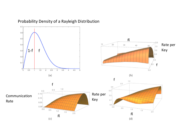
We can integrate over and consider this as a probability distribution over coherent states with , i.e., a Rayleigh distribution:
| (12) |
The median of this distribution is given by , which is a convenient point of separation if we want to send binary messages.
Because the set of coherent states is over-complete, the existence of a coherent-state representation is guaranteed. A related question is how well a set of coherent states with a set of randomly-chosen radii and uniformly random phases can approximate a thermal state. This gives a mixture
| (13) |
The answer is remarkably simple:
| (14) | ||||
where is the average fidelity . This is relevant for “Pairwise” protocols we will discuss later.
Another important bound is on the same kind of setup, but without averaging over . If we instead discretize the circle over —that is, we consider a set of states for sufficiently large —we can do at least as well as the above result. A proof of both these bounds is contained in the appendix.
IV Mappings for Quantum Steganography
In this work we consider four main approaches to encoding information steganographically as states of light: the Fock state encoding, which requires no shared key; an encoding in coherent states without shared key; and two other encodings into coherent states that do require shared key: the Vertical Angles encoding and the Redefined Rayleigh Distribution encoding.
IV.1 Fock State Methods
The scheme for Fock state methods is straightforward and has one clear advantage: Fock states are more easily distinguishable than coherent states, so the communication capacity is higher, although the problem of realizing an arbitrary Fock state in an experimental setting is also more challenging than for coherent states. The protocol we will describe requires only the preparation of multiphoton Fock states, and may be done using probabilistic operations such as photon addition. As such, it can in principle be done using only single photon sources, single photon detectors, and beam splitters, although when is high this may become experimentally difficult due to low observation probability. It should be noted that in that regime, the coherent state methods described in this paper perform more competitively with the Fock state methods due to the greater ease of distinguishing between different coherent states at a higher amplitude. This method, however, requires an encoding system from binary digits to Fock states which depends on the value of , and is described in detail in Section VI and the Appendix. If we are dealing with Fock states in a noiseless channel, the problem is one of translating regular binary strings into binary strings with a certain number of 1s and 0s determined by . It is worth noting as an experimental consideration that, in cases where is low, the weight of the encoded text will be low on average and a sophisticated encoding may not be necessary. In cases where is very large, that may not be the case, and it would require us to define different Fock states as encoding the binary 1 or 0, according to the Boltzmann weights of such Fock states (for example, we might define all states below a certain value of as belonging to 0, and the others to belong to 1). In Section VI we will consider a more intermediate case for communication of a message of length bits and derive bounds on its efficiency.
IV.2 Distribution Coherent State Methods
Since Equation 14 describes the average fidelity, it makes sense to examine different approaches to optimize this quantity, taking into account the non-orthogonality of the coherent states being measured. In all cases we will draw from distributions defined by
| (15) |
representing the transmission of 0 and 1 from the sender.
First, we consider the “distribution” case, which does not require key, where Alice draws a coherent state randomly from or and Bob has to try and guess which distribution it came from. Bob’s ability to do this is bounded by the trace distance between the states and . This is difficult to evaluate, but can be evaluated in terms of the cumulative distribution function of the Poisson processes,
| (16) |
for a process with and for , with the median of the Poisson process (a full derivation is included in the appendix):
| (17) | ||||
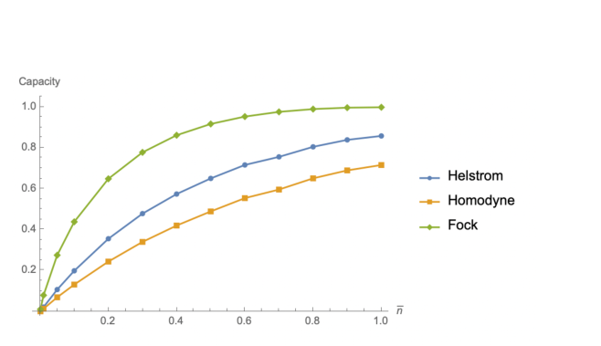
From this we can calculate the probability of error and the communication rate . Since the Poisson process is discrete, this curve has some kinks when increases, as seen in figure 1. When is large, the states and are almost orthogonal; but when is or smaller, the two states have significant overlap and are not perfectly distinguishable. In this case error correction may be necessary, and matching the thermal state may still require shared secret key, as discussed in Section VI. We consider two variations of this idea below.
IV.3 Pairwise Coherent State Methods
A related method is to partition the thermal state as above and select a finite set of states from each half to send. As we showed above, this finite set approximates the thermal state very well and can be distinguished more easily from each other. This method may be easier to implement practically, as only sampling from a subset of is sufficient, but requires more secret key than the distribution methods, which will be quantified in Section VI.
IV.4 Vertical Angles
In this approach, Alice and Bob choose and ahead of time to have opposite phases , i.e. and , where can be chosen arbitrarily. These states correspond to the binary 0 or 1 and are drawn from the distributions and , although since this specific protocol is more useful for the low- case, will likely be sampled more often. Knowledge of the two possible states constitutes a secret key, and the correlation helps distinguish the distributions by minimizing the overlap
This is maximized for , which gives
| (18) |
| (19) | ||||
The associated communication rate is which can be seen in figure 1.
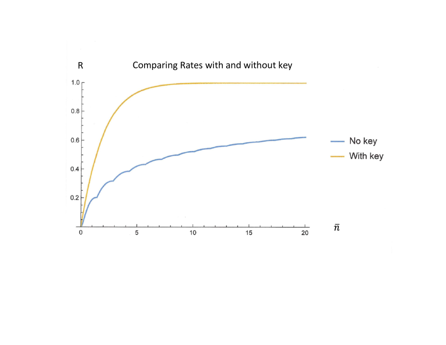
We can think of this setup as using a key, since Alice and Bob must have prior information linking the two values, in contrast to the aforementioned no-key case. Using this key allows a greater rate of communication, since the overlap between the coherent states representing 0 and 1 is minimized. We can see this in figure 1.
IV.5 Redefined Rayleigh Distributions
The final approach involves simply drawing and from the corresponding distributions, communicating them over a channel, and attempting to determine which distribution was sampled from based on the channel measurement. This approach is equivalent to determining the overlap of the distributions and , where we are once again randomizing , but the two are not simultaneously diagonal in any basis and so the optimal measurement to distinguish them is not easy to find with no key. In this section we consider a specific type of measurement and attempt to optimize for a variable parameter which will distinguish between the two states and , although in Section VI we will also consider measurements that saturate the Helstrom bound Helstrom
| (20) |
when discriminating between two states and occurring with probabilities and , respectively.
There is one notable difference between this approach and the previous. For easy distinction, we can without loss of generality choose for our analysis and redefine the distribution as spanning to make it easier to distinguish from , as this essentially rotates about the origin by and creates the greatest possible distance between the means and medians of and by such an operation, while not fundamentally changing the nature of any calculations we will perform.
IV.5.1 Setup
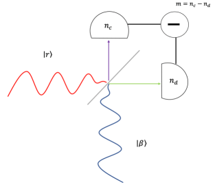
The coherent state-based protocols we are considering use a balanced homodyne measurement of a state . This state is coupled to an oscillator by means of the beam splitter shown in figure 2. If we have the operators and , of which is an eigenket of , and likewise and for , once the states pass through the beam splitter the outcome is characterized by the new operators and . As such, the desired observable is given by .
IV.5.2 Bounds
We can derive bounds using the generalized Markov inequality,
| (21) |
for even , where is a random variable, is its mean, and is its th moment.
Applying this to the distributions for and , we have for a cutoff value that
| (22) | |||
where here and refer to the mean expected values for each distribution, and , respectively.
There is an explicit formula:
| (23) |
We also have the explicit formula for moments of , under the approximation (since only the leading order terms in matter for sufficiently large real ):
| (24) | ||||
where
| (25) |
A derivation of the above is obtained by acting with and equating the Taylor expansions of both sides to each order in . This provides a means to evaluate the higher-moment Markov bound
| (26) | ||||
V Numerical simulation and performance
We expect that for a coherent state, the distribution of will be Gaussian OCW . It is straightforward to compute the mean and variance of in the case where is randomly sampled from the distributions without constraint, rather than being one of two possibilities:
| (27) | ||||
Likewise,
| (28) | ||||
Sampling from a normal distribution with these parameters is simple, so we can empirically determine the optimal value of by simulating the transmission homodyne measurement procedure directly. The results are displayed in figure 3.
The above refers to the case where is randomly sampled from the distributions without constraint, rather than being one of two possibilities. In latter case, where the key designates one of two specific states to be distinguished between by homodyne measurement for each transmitted bit (one state from and one from ), the optimal value calculation for is more straightforward—it derives from optimizing the accumulated probability
| (29) |
at —and gives the result
| (30) | |||
which does not exceed 1/2. We will compare this to the Helstrom bound once we derive a bound for Fock state communication in Section VI, so they can all be seen side-by-side.
VI Particular Encoding Methods
VI.1 Fock State Methods
Continuing from the discussion in section IV, if we denote any Fock states with as the binary 1, we must have a quantity of 0s and 1s in the encoded string, which comes directly from the Fock state representation of . Thus the problem is one of encoding from the set of all binary strings of length to the set of binary strings with such a ratio, of which there are . It is straightforward to calculate the channel capacity using such an encoding, as the number of bits we can encode is simply —this provides evidence for the simplicity of the cases of extreme as noted in section IV.
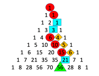
We can approach this rate using a “by value” encoding. Think of an -bit string as representing an integer , and encode this as the th smallest bit string (by value) that satisfies the above criteria for the number of 0s and 1s. We can use a theorem called the “Christmas Stocking Theorem” christmas to efficiently generate the encoding, going from either the least or most significant bit. This theorem states that
| (31) |
which provides a straightforward way of counting down digits. More details and examples are contained in the appendix.
VI.2 Coherent State Methods
We want to emulate the statistics of the thermal state using coherent states sampled from our distributions, and . If we have an equal number of 0s and 1s in the message, this is straightforward: we can sample from the distributions and simply transmit the result. There is a catch, however: since the coherent states are not orthogonal, there is a probability of mistaking for at the time of measurement, which produces something similar to a Pauli X error. We can protect against this by using error correction and encoded keywords; however, this requires secret key, since the encoded messages will no longer appear to be sampled from .
For example, if we use a simple 3-bit Hamming code, there are only 2 codewords (000 and 111) and 8 possible, equally-likely bit-strings we would expect to see if sampling from . We can make these strings appear random again by doing a bitwise XOR with a random 3-bit string, selected by generating a random number between 0 and 7. This scrambled codeword will still protect against a bit-flip error, but it requires that Bob also know the random number that was chosen. So such a scheme requires Alice and Bob to share a secret key in advance. If we wish to cut down on the amount of secret key used, we could use a shared seed for a pseudorandom number generation protocol, such as the rabbit cipher, which is thought to be cryptographically secure rabbit . However, this would reduce the secrecy below the information-theoretic level we have been assuming up to this point.
VI.2.1 Distribution Method
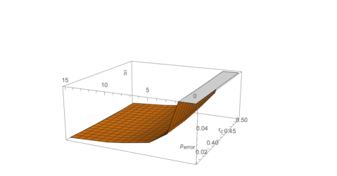
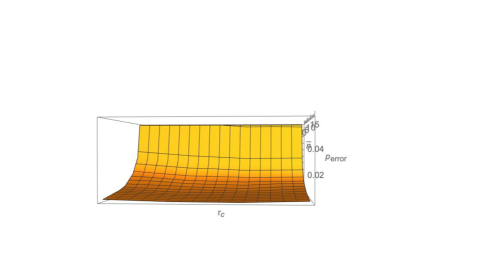
We can quantify the results of the coherent state encoding. Supposing that, instead of splitting the coherent distribution in half radially, we split it so that a fraction of the density is on the right and denotes a binary 1, and a fraction on the left denotes the binary 0, we can find the optimal communication rate in terms of . The results in Fig. 4 show that asymptotically, no secret key is needed for sufficiently large , when we use an -value closer to 0. Interestingly, there is a trade-off between the optimal communication rate in terms of minimizing , and making the states as easy as possible to disguise. The key rate required here is given by
| (32) | ||||
where the probabilities refer to the probability that Bob measures a state he decides is from given that Alice sent a state from . We will derive expressions for these quantities below.
VI.2.2 Pairwise Method
We can also consider this approach from the perspective of using a finite set of states—what we called the “pairwise” protocol earlier. If we use a set of size , with drawn from and drawn from , we should still maintain a fidelity scaling of , since the overall statistics are still the same as before.
If we add factors of in front of and in front of in the expression we previously derived in 30 for under homodyne measurement, with these weightings we now have
| (33) |
and
| (34) | |||
We see that for the value of reverts to .
For optimal generalized (Helstrom) measurements, we consider the quantity
| (35) |
If we orthogonalize the basis using , we can express this as
| (36) | |||
with
| (37) |
Then we have that in this basis
| (38) | ||||
where is the eigenvector of corresponding to the eigenspace.
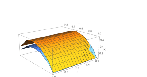
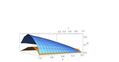
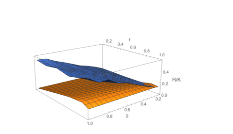
From these quantities we can roughly determine the rate of this communication method, which is limited by the entropy difference between the encoded and decoded information:
| (39) |
and the key rate is set by the entropy difference between a simulated binary symmetric channel and the mutual information of the actual channel
| (40) |
where . Then, we can plot the associated quantities, such as , , and , and we see in Fig. 5 that the ratio is fairly small for the homodyne measurement case but not for the Helstrom case.
We will also need additional shared secret key to specify which pair of states is being used for each transmitted bit. To specify a pair of states, one for each bit value, requires an additional bits of key. The communication rate, however, remains the same as described above. Note that the asymptotic communication rate per bit of key can be demonstrated analytically to exceed 1 by examining the limiting behavior of the expression for .
Note that the value of manifests itself in the specific coherent states that will be drawn from the distributions, rather than being directly visible in the binary transmitted bits as in the Fock case. If the message does not contain a roughly equal number of 1s and 0s, we can use an encoding, such as the one described in the appendix, to compensate for that. However, in that case the message should first be compressed, which increases the entropy of the transmitted string; and if need be, a sublinear amount of secret key can be used to make the message string indistinguishable from a purely random bit string noichris ; noilchris .
VII Discussion and Future Work
As we can see, the Fock state encoding is superior in the noiseless case and also doesn’t require key. Moreover, it is straightforward and the encoding has a clean visual representation based on Pascal’s triangle (as shown in the Appendix). However, coherent states are more resistant to noise and are easier to generate in the lab, although they perform noticeably worse under either ideal (Helstrom limit) or homodyne measurements. In both cases, however, it is viable to communicate information covertly using the above-described methods for any channel parameter , and even in the coherent case the amount of secret key required is low compared to, for example, a one-time pad.
There are many possible future directions to explore to build on this work. An interesting problem is that of modeling noisy channels—for example, one with an existing thermal noise background—and the transmission of coherent states through such a channel (which is a well-understood problem) Vourdas . Such a study would provide a more thorough grounding for this work’s study of coherent state methods, which are suboptimal in the noiseless case we have examined.
Another important problem is that of transmitting quantum information, including entanglement. In this work we have only considered classical information transmission. It is unclear what kinds of encodings can be used for quantum information and how well they preserve the entanglement of the system, both in the noisy and the noiseless case. Such a work might also delve into the potential applications of this communication method to teleportation and superdense coding protocols, for example, and methods of making those more secure under the type of schemes covered in this paper.
A final promising area of study could be different key utilization protocols, with the goal of utilizing the inherent noise protection assumptions of steganography to efficiently scale the encryption process, and using other quantum communications as a vehicle for encoding steganographic information. This aims to get around this work’s requirement that secret key is needed for non-orthogonal state discrimination by exploiting the information difference between Alice, Bob, and Eve to communicate a secret key seed, without compromising the communication rate derived above.
Acknowledgements
The authors would like to thank Jonathan Habif and Haley Weinstein for helpful discussions and insights. This research was supported in part by NSF Grants 1719778 and 1911089.
References
- (1) Wobst, Reinhard (2001). Cryptology Unlocked. Wiley. p. 19.
- (2) Simmons, Gustavus J.. “Vigenère cipher”. Encyclopedia Britannica, 25 Feb. 2023, https://www.britannica.com/topic/Vigenere-cipher. Accessed 28 February 2023.
- (3) Bruen, Aiden A. & Forcinito, Mario A. (2011). Cryptography,Information Theory, and Error-Correction: A Handbook for the 21st Century. John Wiley & Sons. p. 21.
-
(4)
“Origin of Cryptography.” Origin of Cryptography, https://www.tutorialspoint.com/cryptography
/origin_of_cryptography.htm. - (5) Abdulrazzaq, S.T., Siddeq, M.M. & Rodrigues, M.A. A Novel Steganography Approach for Audio Files. SN COMPUT. SCI. 1, 97 (2020). https://doi.org/10.1007/s42979-020-0080-2
- (6) M. Dušek, N. Lütkenhaus, M. Hendrych, Quantum cryptography, Progress in Optics 49 (2006) 381–454.
- (7) Chip Elliott, David Pearson and Gregory Troxel. Quantum Cryptography in Practice, 2003; arXiv:quant-ph/0307049.
- (8) S. Pirandola, U. L. Andersen, L. Banchi, M. Berta, D. Bunandar, R. Colbeck, D. Englund, T. Gehring, C. Lupo, C. Ottaviani, J. L. Pereira, M. Razavi, J. Shamsul Shaari, M. Tomamichel, V. C. Usenko, G. Vallone, P. Villoresi, and P. Wallden, “Advances in quantum cryptography,” Adv. Opt. Photon. 12, 1012-1236 (2020)
- (9) Bash, B., Goeckel, D. & Towsley, D. Square root law for communication with low probability of detection on AWGN channels. 2012 IEEE International Symposium On Information Theory Proceedings. pp. 448-452 (2012)
- (10) Boulat A. Bash, Dennis Goeckel and Don Towsley. Covert Communication Gains from Adversary’s Ignorance of Transmission Time, 2014; arXiv:1403.1013.
- (11) J. Gea-Banacloche, J. Math. Phys. 43, 4531 (2002).
- (12) M. Curty, D. J. Santos, paper presented at the 2nd Bielefeld Workshop on Quantum Information and Complexity, Bielefeld, Germany, 10 October (2004).
- (13) Tahmasbi, M., & Bloch, M. R. (2020). Steganography protocols for quantum channels. Journal of Mathematical Physics, 61(8), 082201. doi:10.1063/5.0004731.
- (14) Bilal A. Shaw and Todd A. Brun. Hiding Quantum Information in the Perfect Code, 2010; arXiv:1007.0793.
- (15) Shaw, B. A., & Brun, T. A. (2011). Quantum steganography with noisy quantum channels. Physical Review A, 83(2). doi:10.1103/physreva.83.022310.
- (16) Ben Wu, Zhenxing Wang, Yue Tian, Mable P. Fok, Bhavin J. Shastri, Daniel R. Kanoff, and Paul R. Prucnal, “Optical steganography based on amplified spontaneous emission noise,” Opt. Express 21, 2065-2071 (2013)
- (17) Riaz, A., & Ali, M. (2008). Chaotic Communications, their applications and advantages over traditional methods of communication. 2008 6th International Symposium on Communication Systems, Networks and Digital Signal Processing. doi:10.1109/csndsp.2008.461080
-
(18)
An Introduction to Spread Spectrum Techniques. https://www.ausairpower.net/OSR-0597.html#: :text=Security%20from%20Eavesdropping.
,almost%20perfect%20immunity%20to%20interception.
Accessed 19 Aug. 2023. - (19) Shi, H., Zhang, Z. & Zhuang, Q. Practical Route to Entanglement-Assisted Communication Over Noisy Bosonic Channels. Phys. Rev. Appl.. 13, 034029 (2020,3)
- (20) Fuchs, C. A. & van de Graaf, J. (1998). Cryptographic distinguishability measures for quantum mechanical states. IEEE Transactions on Information Theory 45(4), 1216–1227. arXiv:quant-ph/9712042.
- (21) Vourdas, A. Optical signals with thermal noise. Phys. Rev. A. 39, 206-213 (1989,1), https://link.aps.org/doi/10.1103/PhysRevA.39.206
- (22) C. W. Helstrom. Quantum detection and estimation theory. Academic Press, New York, 1976.
- (23) Jeffrey H. Shapiro, 6.453 Quantum Optical Communication. Fall 2016. Massachusetts Institute of Technology: MIT OpenCourseWare, https://ocw.mit.edu/. License: Creative Commons BY-NC-SA.
-
(24)
Weisstein, Eric W. “Christmas Stocking Theorem.” From MathWorld–A Wolfram Web Resource. https://mathworld.wolfram.com/
ChristmasStockingTheorem.html - (25) Boesgaard, M., Vesterager, M., Pedersen, T., Christiansen, J., Scavenius, O. (2003). Rabbit: A New High-Performance Stream Cipher. In: Johansson, T. (eds) Fast Software Encryption. FSE 2003. Lecture Notes in Computer Science, vol 2887. Springer, Berlin, Heidelberg. https://doi.org/10.1007/978-3-540-39887-5_23
- (26) Arsal, A. A STUDY ON WIRELESS CHANNEL MODELS: SIMULATION OF FADING, SHADOWING AND FURTHER APPLICATIONS. (2008,8)
- (27) Sutherland, C. & Brun, T. Quantum steganography over noisy channels: Achievability and bounds. Phys. Rev. A. 100, 052312 (2019,11), https://link.aps.org/doi/10.1103/PhysRevA.100.052312
- (28) Sutherland, C. & Brun, T. Quantum steganography over noiseless channels: Achievability and bounds. Phys. Rev. A. 101, 052319 (2020,5), https://link.aps.org/doi/10.1103/PhysRevA.101.052319
*
Appendix A
A.1 Proof of Eq. (14)
We start from the fidelity between
| (41) |
and the thermal state :
| (42) |
If we define the quantity , then we know immediately that since . Then since , we can write
| (43) |
which can be lower-bounded by taking the binomial expansion of the square root. We can then take the ensemble average:
| (44) | ||||
where here
| (45) |
We have that the are independent and that for each one , so if we consider the cases only where all are equal, which we’ll call , we have
| (46) |
which makes the result of Eq. (44)
| (47) |
We can now finally evaluate this trace term:
| (48) | ||||
where we have used that
| (49) |
This makes the final result of Eq. (44)
| (50) |
in the average case.
A.2 Discretizing the Circle
The second bound is when the circle is discretized over . This encoding gives us that for and and
| (51) |
Then we have
| (52) | ||||
since the geometric series sums to . We can now evaluate the fidelity:
| (53) | ||||
This gives the same bound as before:
| (54) |
If we instead consider the distributions and , we can easily show, at least, that as (since the integrals over the distributions are hard to compute) starting from Eq. (44):
| (55) | ||||
A.3 Derivation of Vertical Angle Bound with no Key
We start with the two states, given :
| (56) | ||||
and
| (57) | ||||
The fidelity between these two states is given by
| (58) |
where is the th cumulant of the Poisson process with parameter .
We can rewrite the trace distance as
| (59) | |||
where is such that iff .
We take each term in the sum in turn:
| (60) | ||||
where is the CDF for the Poisson process with .
The second sum is
| (61) | ||||
Combining these sums gives us the final result:
| (62) |
A.4 Encoding Method for Fock States
Elaborating on the results of Section V, we can imagine a particular encoding method for Fock state communication. Let’s consider a particular example. Suppose and Alice wants to communicate the six-bit string 101001, which we can think of as the binary expression for the number 41. (Note that this protocol requires Bob to know the size of the message being communicated). If Alice wants to know how many bits she needs to encode an -bit number with zeroes, she solves the equation
| (63) |
Alice can transmit her string with bits: the condition is that
| (64) |
where we use to denote the value of the message, which is 41. Therefore, Alice’s message should consist of 5 bits of 0, 3 bits of 1, and we can verify that .
As we will show, 41 is encoded by the binary string 10001100, which is the binary expression for 140, the -smallest number with an 8 bit string representation (possibly with leading zeroes) with the appropriate ratio of 1s to 0s. To find this string, we follow a process derived from the “Christmas Stocking Theorem” mentioned above, which we detail in figure 7. First, consider that if we are using bits, of which are 0, there are strings with 1 in the first spot. There are strings with 0 in the first spot and 1 in the second spot. And so on. Alice can subtract these from total possible strings to find the string in question. For example, the first bits have a 1 at the start, and so Alice’s message must start with 1, denoted by the blue square over the 21 in the figure. Then there are strings with 11, so the second bit she sends must be 0, since (denoted by the red square over the 6 in the figure). so the string so far is 10001. Actually, at this point we have reached the largest string so Alice’s message is the largest such string with that prefix, 10001100=140, and the remaining digits are in red in the figure since they correspond to the trailing 0s now that we have allocated all the 1s.
Once Alice knows that this is the encoded string she wants to send, she generates 8 Fock states in a ratio of 5:3 zeroes to ones (where “one” here refers to a mode greater than 0, with the appropriate statistics to emulate the thermal state). Then she sends one of the states for every position corresponding to 1 in the string 10001100 and a state for each 0. Bob measures the Fock states and should receive 1001100 as the most likely string, after inverting the above algorithm, which is straightforward. Eve should see something that looks like a thermal state: after all, it is bitwise random and has the required overall statistics.
A.5 Practical Fidelity Bounds for the Fock Encoding
In practice, the Fock state encoding is not exactly equivalent to a thermal state. While we would like to send the state
| (65) |
in practice we have a finite number of bits, so we are sending either the state
| (66) |
or the state
| (67) |
(whichever maximizes the fidelity). Another way of writing this is, e.g.,
| (68) | ||||
We would like to compute, as a function of ,
| (69) | ||||
where the third order correction is due to Taylor’s theorem. The above chain of inequalities shows that when is fairly large, the fidelity between the encoded state and the thermal state is very close to 1. At the cost of sharing some additional secret key, Alice and Bob can actually make the fidelity (almost) perfect. The gap in fidelity between the encoded state and the thermal state results from using integer approximations to and . But Alice and Bob can, in principle, randomly choose the numbers of 0s and 1s to be used in the encoding, from the binomial distribution with probabilities corresponding to the thermal state: and . By averaging over this choice, one can match the thermal state perfectly.