An Information-Theoretic Characterization of MIMO-FAS: Optimization, Diversity-Multiplexing Tradeoff and $q$-Outage Capacity

Abstract

Multiple-input multiple-output (MIMO) system has been the defining mobile communications technology in recent generations. With the ever-increasing demands looming towards the sixth generation (6G), we are in need of additional degrees of freedom that deliver further gains beyond MIMO. To this goal, fluid antenna system (FAS) has emerged as a new way to obtain spatial diversity using reconfigurable position-switchable antennas. Considering the case with more than one ports activated on a 2D fluid antenna surface at both ends, we take the information-theoretic approach to study the achievable performance limits of the MIMO-FAS. First of all, we propose a suboptimal scheme, referred to as QR MIMO-FAS, to maximize the rate at high signal-to-noise ratio (SNR) via joint port selection, transmit and receive beamforming and power allocation. We then derive the optimal diversity and multiplexing tradeoff (DMT) of MIMO-FAS. From the DMT, we highlight that MIMO-FAS outperforms traditional MIMO antenna systems. Further, we introduce a new metric, namely $q$-outage capacity, which can jointly consider rate and outage probability. Through this metric, our results indicate that MIMO-FAS surpasses traditional MIMO greatly.

I Introduction

I-A Background

Sixth-generation (6G) mobile communication seeks to push the key performance indicators (KPIs) way beyond what the current fifth generation (5G) promises to offer. Such upgrade will require new technologies that can achieve more from the same amount of bandwidth. Presently, the dominating technology has been multiple-input multiple-output (MIMO), which also comes in the form of multiuser MIMO and massive MIMO. In 6G, the desire is to exceed MIMO [1, 2].

To achieve this very ambitious goal, one emerging idea is fluid antenna system (FAS) [3]. FAS represents any software-controllable fluidic, conductive or dielectric structure that can adjust its shape and position to reconfigure the gain, radiation pattern, operating frequency and other radiation characteristics. This is now feasible, thanks to the recent advances in utilizing flexible conductive materials such as liquid metals or ionized solutions [4], switchable pixels [5, 6], and stepper motors for antennas [7, 8]. The concept of fluid antenna includes all forms of movable and non-movable flexible-position antennas.

Unlike traditional antenna that is placed at a fixed location, fluid antenna is able to switch its location almost instantly in a limited space. The most basic single fluid antenna consists of one radio frequency (RF)-chain and $N$ preset locations (also known as ports) that are distributed in a given space [3]. The radiating element of the fluid antenna can switch its position to obtain a higher rate, lower outage probability, less interference and other desirable performance gains depending on the applications. As the ports can be placed closely to each other, the channels of these ports are strongly correlated and thus spatial correlation plays a crucial role in FAS.

The main implementation designs for FAS are: i) liquid-based fluid antenna and ii) RF pixel-based fluid antenna. In the liquid-based fluid antenna, each liquid droplet can precisely switch its position by controlling the electric field using the thin conductive lines on top of the dielectric layer while other technology may use an electronically controlled pump to shift the position of a fluid radiating element in a tube. On the other hand, in the RF pixel-based fluid antenna, the RF pixels can be turned on-and-off instantly regardless of the surface area. One or several pixels when on, form an antenna port for transmission or reception like a standard antenna. Besides, each activated port is connected to an RF-chain, operating like a conventional antenna. In short, the basic principle of FAS is to exploit the dynamic nature of fluid antenna to achieve ultimate flexibility for diversity and multiplexing gains.

Due to its unprecedented benefits, single-user, single-input single-output (SISO)-FAS has recently been investigated under different scenarios and assumptions. Specifically, as the number of ports increases, [9] showed that the outage probability of FAS could be reduced drastically while [10] demonstrated that FAS could significantly improve the ergodic capacity. Motivated by these works, [11] derived the level crossing rate, [12] devised a port selection algorithm by observing the channels of a few ports, [13] investigated the performance of FAS over general correlated channels and [14] analyzed the outage probability of FAS for Terahertz communications while selection combining and maximum gain combining were further considered. Optimistic results were obtained in these works but it was illustrated in [15] that the outage probability of FAS could only be reduced to a floor when a more accurate spatial correlation model was adopted. The recent work [16] explained such limitations at an intuitive level and revealed that the performance of FAS was generally determined by the available space. Furthermore, only in certain cases might FAS achieve a similar outage probability as compared to the classical maximal ratio combining (MRC) system.

The unique ability of switching the antenna position finely in FAS can also be exploited to mitigate interference, which would be impractical in traditional antenna selection systems. Recently, [17] investigated orthogonal multiple access to serve multiple users with fluid antennas while [18] used a space division multiple access approach to minimize the user transmit power. Nevertheless, an arguably more interesting idea is the fluid antenna multiple access (FAMA) scheme [19] where the rationale is to exploit the moment of deep fades in the spatial domain to alleviate inter-user interference. FAMA is classified into slow FAMA and fast FAMA in which the former switches its port when the channel changes [20] and the latter switches its port on a symbol-by-symbol basis [21]. Most recently, the outage probability for two-user FAMA was revisited in [22].

In summary, FAS has shown promises but much is still not well understood. For example, the performance of FAS itself can be lifted if more than one ports are activated. For a point-to-point communication channel, we refer to the system where both ends are equipped with a multi-port FAS, as MIMO-FAS which is also known as fluid MIMO or flexible MIMO in [3]. Note that multiple ports can also be activated in a two dimensional (2D) surface using liquid-based fluid antenna or RF pixel-based fluid antenna. The schematics of the MIMO-FAS designs were discussed in [3]. Compared to a traditional MIMO antenna selection system in which the number of antennas is limited in a given surface (at least half wavelength separation between the antennas) and the antennas are fixed in positions, MIMO-FAS is distinct in the sense that the positions of the radiating elements can be dynamically and finely adjusted and that the number of preset locations (i.e., ports) within a given surface can be arbitrarily large, which yields additional gains. Note that FAS has also been proposed for multiple access recently [20, 21, 22], where the fine resolution of FAS is absolutely essential and conventional antenna selection would be unable to cope.

It is anticipated that the capacity and reliability of MIMO-FAS will be improved over the SISO counterpart. In fact, a related work showed that the capacity of a movable antenna system (which can be interpreted as MIMO-FAS with movable fluid antennas) could be improved up to $30.3\%$ as compared to traditional MIMO systems [23]. In the study, however, spatial correlation due to rich scattering between the antenna positions was not considered. More importantly, the optimal diversity and multiplexing tradeoff (DMT) of MIMO-FAS is unknown.

In information theory, the optimal DMT can be employed as a unified framework to compare the performance of different multiple-antenna systems [24]. More concretely, it focuses on the asymptotic high signal-to-noise ratio (SNR) regime and a scheme is then said to achieve a multiplexing gain of $r$ and a diversity gain of $d\left(r\right)$ if the rate of the system scales like $r\log{\rm SNR}$ and its outage probability decays like ${\rm SNR}^{-d\left(r\right)}$. It is known that $r$ cannot exceed the total degrees of freedom of the channel and $d\left(0\right)$ is limited by the maximal diversity gain, i.e., total number of independent channels. In between the two extremes, a system must tradeoff each type of gains.

I-B Contributions

Motivated by the above, this paper analyzes the performance of MIMO-FAS with the goal of gaining useful insights for designing an efficient MIMO-FAS. To this end, we first develop a system model of MIMO-FAS while taking into account of the spatial correlation effect. To characterize the performance limits of MIMO-FAS, we consider a rich scattering environment since it is well known that multipath can help to improve the diversity and multiplexing gains. We then propose a suboptimal scheme that maximizes the rate of MIMO-FAS through joint port selection, transmit and receive beamforming and power allocation at high SNR. Based on this scheme, we derive the optimal DMT of MIMO-FAS to reveal the fundamental limits of MIMO-FAS from an information-theoretic viewpoint. From the analytical results, we further study the effects of different MIMO-FAS parameters and reveal the superiority of MIMO-FAS over traditional MIMO and MIMO antenna selection in terms of DMT. In addition, we introduce a new metric, referred to as $q$-outage capacity, to showcase the benefits of MIMO-FAS. Our main contributions are summarized as follows:

• We develop a system model for MIMO-FAS with a 2D fluid antenna surface at both ends while taking into account of the spatial correlation of the ports. In particular, we employ a simple yet accurate channel model that considers the spatial correlation in a three-dimensional (3D) scattering environment. Based on this channel model, we introduce several system parameters such as active ports, beamforming matrices and power allocation. The achievable rate of MIMO-FAS is then derived where its expression resembles the rate of a traditional MIMO system.

• Also, we formulate a non-convex optimization problem to maximize the rate of MIMO-FAS via joint port selection, transmit and receive beamforming and power allocation. We show that the global optimal solution can be obtained using an exhaustive search, singular value decomposition (SVD) and waterfilling power allocation, at the expense of a non-polynomial time complexity. To reduce the time complexity, we propose the QR MIMO-FAS scheme that maximizes the rate of MIMO-FAS at high SNR via suboptimal port selection, beamforming and power allocation. It is shown that QR MIMO-FAS has a polynomial time complexity.

• Furthermore, we derive the outer bound of the DMT of MIMO-FAS. By using the outer bound and QR MIMO-FAS, we obtain the optimal DMT of MIMO-FAS. In this process, we prove that the spatial correlation matrix $\boldsymbol{J}_{s}$ can be represented by a finite-size matrix $\boldsymbol{J}_{{\rm red}}^{s}$ even if the number of ports increases to infinity. Afterwards, we propose methods to estimate the size of $\boldsymbol{J}_{{\rm red}}^{s}$ and linearly transform between $\boldsymbol{J}_{s}$ and $\boldsymbol{J}_{{\rm red}}^{s}$ with proof of certificates.

• Extensive results are provided to highlight the effects of several MIMO-FAS parameters. In the discussions, we provide useful insights for designing an efficient MIMO-FAS. Although MIMO-FAS provides rate improvements over the traditional MIMO antenna systems, we highlight that the superiority of MIMO-FAS actually lies in the diversity gain. Specifically, the diversity gain of MIMO-FAS for a fixed $r$ is much greater than that of MIMO and MIMO antenna selection if the total number of active ports or antennas is the same.

• Finally, we introduce a new performance metric, referred to as $q$-outage capacity, that jointly considers both rate and outage probability. We show that MIMO-FAS outperforms the traditional MIMO and MIMO antenna selection in terms of $q$-outage capacity. This result suggests that MIMO-FAS is more reliable in delivering high data rate transmission than the traditional MIMO systems.

I-C Organization and Notations

The remainder of this paper is organized as follows. Section II introduces the system model of MIMO-FAS. Section III details the proposed QR MIMO-FAS scheme that maximizes its rate at high SNR. The optimal DMT of MIMO-FAS is analyzed in Section IV. Section V presents the numerical results to compare MIMO-FAS with the traditional MIMO systems and we conclude the paper in Section VI.

Table I: The meanings of key notations.

Notation	Meaning
$\boldsymbol{A}$	Activation port matrices at both of the transmitter and receiver sides
$\boldsymbol{A}_{s}$	Activation port matrix at side $s$
$C_{{\rm sys}}^{q}$	$q$-outage capacity of a system
$d\left(r\right)$	Diversity gain for $r$ multiplexing gain
$\boldsymbol{G}$	Circularly symmetric complex Gaussian matrix with i.i.d. entries
$\boldsymbol{H}$	Complex channels of MIMO-FAS
$\overset{}{\bar{\boldsymbol{H}}}$	Complex channels of the activated ports
$\boldsymbol{H}_{a}$	Partial channels of the active ports
$\boldsymbol{H}_{i}$	Partial channels of the inactive ports
$\boldsymbol{J}_{s}$	Spatial correlation matrix at side $s$
$\hat{\boldsymbol{J}}_{s}$	Approximated matrix of $\boldsymbol{J}_{s}$
$\boldsymbol{J}_{{\rm red}}^{s}$	Full rank spatial correlation matrix at side $s$
$\boldsymbol{K}$	Input covariance
$n_{s}$	Total number of active ports
$n_{{\rm{max}}}/n_{{\rm{min}}}$	Maximum/minimum of $n_{rx}$ and $n_{tx}$
$N_{{\rm{max}}}/N_{{\rm{min}}}$	Maximum/minimum of $N_{rx}$ and $N_{tx}$
$N_{s}$	Total number of ports at side $s$
$N_{i}^{s}$	Number of ports in the $i$-th dimension at side $s$
$N_{s}^{{}^{\prime}}$	Rank of $\boldsymbol{J}_{{\rm red}}^{s}$
$N_{\min}^{{}^{\prime}}$	Minimum of $N_{rx}^{{}^{\prime}}$ and $N_{tx}^{{}^{\prime}}$
$P_{{\rm sys}}^{{\rm out}}\left({\rm SNR},r\right)$	Outage probability of a system in terms of $r\log{\rm SNR}$
$\bar{P}_{{\rm sys}}^{{\rm out}}\left({\rm SNR},q\right)$	Outage probability of a system for a fixed $q$-transmission rate
$\boldsymbol{P}$	Power allocation matrix
$r$	Multiplexing gain
$R_{{\rm sys}}\left({\rm SNR}\right)$	Rate of a system for a given ${\rm SNR}$
$s\in\left\{tx,rx\right\}$	Subscript/superscript to denote the transmit/receiver side
${\rm SNR}$	Transmit SNR
$\boldsymbol{v}_{l}^{s}$	Certificate between the linear transformation of $\boldsymbol{J}_{s}^{\left(l\right)}$ and $\boldsymbol{J}_{{\rm sub}}^{\left(l-1\right)}$
$W_{s}$	Total area of the fluid antenna at side $s$
$W_{i}^{s}$	Length of the fluid antenna in the $i$-th dimension at side $s$
$\boldsymbol{W}$	Transmit and receive beamforming matrices
$\boldsymbol{W}_{s}$	Beamforming matrix at $s$ side
$\lambda$	Wavelength of the carrier frequency
$\boldsymbol{\Lambda}_{s}$	Matrix whose diagonal entries are the eigenvalues of $\boldsymbol{J}_{s}$
$\boldsymbol{\Sigma}$	Matrix whose diagonal entries are singular values of $\boldsymbol{H}$
$\overset{}{\bar{\boldsymbol{\Sigma}}}$	Matrix whose diagonal entries are singular values of $\boldsymbol{\bar{H}}$
$\boldsymbol{\Omega}$	Special matrix used for port optimization

Throughout this paper, scalar variables are denoted by italic letters (e.g., $c$), vectors are denoted by boldface italic small letters (e.g., $\boldsymbol{c}$) and matrices are denoted by boldface italic capital letters (e.g., $\boldsymbol{C}$). Additionally, $\left(\cdot\right)^{T}$ denotes transpose, $\left(\cdot\right)^{H}$ denotes conjugate transpose while ${\rm det}\left(\cdot\right)$, ${\rm rank\left(\cdot\right)}$ and ${\rm trace}\left(\cdot\right)$ represent the determinant, rank and trace of a matrix, respectively. Moreover, $\left|\cdot\right|$, $\left\|\cdot\right\|_{2}$ and $\left\|\cdot\right\|_{F}$ denote the absolute, Euclidean norm and Frobenius norm operations, respectively. Furthermore, we use $\log(\cdot)$ to denote logarithm with base 2, $\left[\cdot\right]_{c}^{+}$ outputs the argument that is lower bounded by $c$, $\min\left\{\cdot\right\}$ and $\max\left\{\cdot\right\}$ denote the minimum and maximum value of the argument, respectively. ${\mathbb{E}}[\cdot]$ returns the expected value of the input random quantity, and $\otimes$ denotes the Kronecker product. Finally, $\boldsymbol{e}_{k}$ represents an all-zero vector except the $k$-th entry being unity, ${\rm diag}(\cdot)$ denotes a diagonal matrix whose diagonal entries are the inputs, and $(\cdot)^{{\dagger}}$ denotes the pseudoinverse of an input matrix. To help readers follow the mathematical contents, the meanings of the key variables are listed in Table I.

II System Model

As illustrated in Fig. 1, we consider a point-to-point wireless communication channel in which the transmitter and receiver are equipped with a fluid antenna. To facilitate our discussions, we use the subscript/superscript $s$ to denote the parameters at the transmitter or receiver as $tx$ or $rx$, respectively, i.e., $s\in\left\{tx,rx\right\}$. We assume that the fluid antenna takes up a 2D space with an area of $W_{s}$ and has $N_{s}$ ports spread uniformly over the 2D space. A grid structure is considered where $N_{i}^{s}$ ports are uniformly distributed along a linear space of length $\lambda W_{i}^{s}$ for $i\in\left\{1,2\right\}$, so that $N_{s}=N_{1}^{s}\times N_{2}^{s}$ and $W_{s}=\lambda W_{1}^{s}\times\lambda W_{2}^{s}$, where $\lambda$ is the wavelength of the carrier frequency. In this MIMO-FAS, the transmitter and receiver can only activate $n_{s}$ out of $N_{s}$ ports. Note that for SISO-FAS, $n_{s}=1,\forall s$.

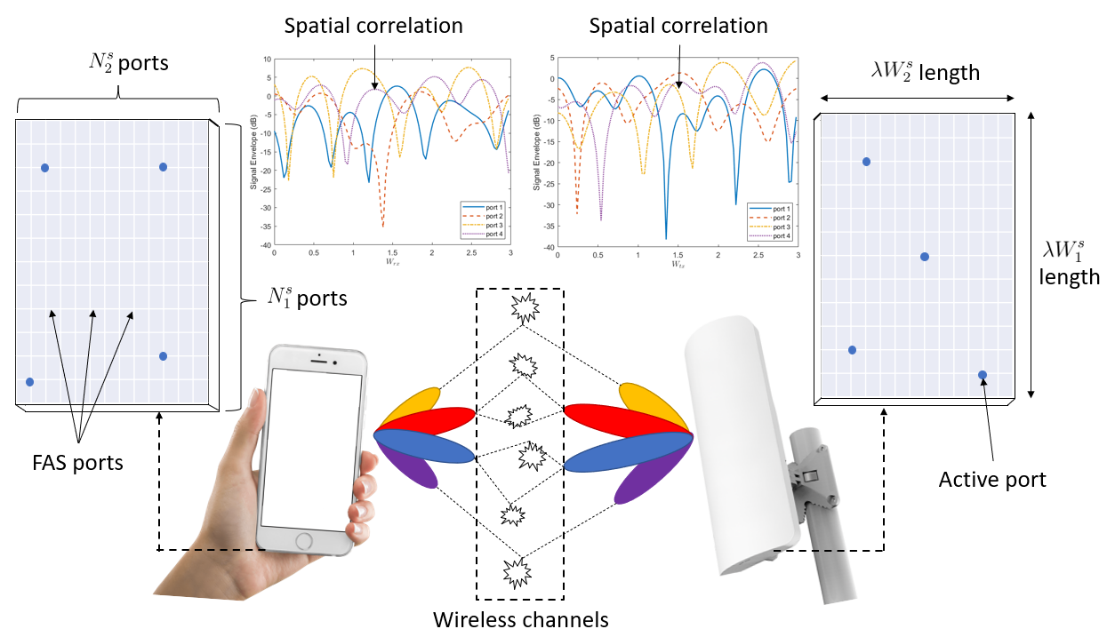
Figure 1: A schematic of point-to-point MIMO-FAS.

Considering a 3D environment under rich scattering, the spatial correlation between the $\left(n_{1}^{s},n_{2}^{s}\right)$-th port and the $\left(\tilde{n}_{1}^{s},\tilde{n}_{2}^{s}\right)$-th port is given by

$$J_{\left(n_{1}^{s},n_{2}^{s}\right),\left(\tilde{n}_{1}^{s},\tilde{n}_{2}^{s}\right)}^{s}$$

$$=j_{0}\left(2\pi\sqrt{\left({\textstyle\frac{\left|n_{1}^{s}-\tilde{n}_{1}^{s}\right|}{N_{1}^{s}-1}W_{1}^{s}}\right)^{2}+\left({\textstyle\frac{\left|n_{2}^{s}-\tilde{n}_{2}^{s}\right|}{N_{2}^{s}-1}W_{2}^{s}}\right)^{2}}\right),$$ (1)

where $j_{0}\left(\cdot\right)$ is the spherical Bessel function of the first kind. A detailed proof can be found in Appendix I. As seen in (1), it is cumbersome to label a port in 2D. To simplify our notations, we use the function ${\rm map}:\mathbb{R}^{2}\rightarrow\mathbb{R}$, e.g., ${\rm map}\left(n_{1}^{s},n_{2}^{s}\right)=l_{s}$, where $l_{s}\in\left\{1,\dots,N_{s}\right\}$.

Using the mapping function, we can express the spatial correlation matrix $\boldsymbol{J}_{s}$ as

$$\boldsymbol{J}_{s}=\left[\begin{array}[]{cccc}J_{1,1}^{s}&J_{1,2}^{s}&\ldots&J_{1,N_{s}}^{s}\\ J_{2,1}^{s}&J_{2,2}^{s}&\ldots&J_{2,N_{s}}^{s}\\ \vdots&\vdots&\ddots&\vdots\\ J_{N_{s},1}^{s}&J_{N_{s},2}^{s}&\ldots&J_{N_{s},N_{s}}^{s}\end{array}\right],$$ (2)

where $J_{k_{s},l_{s}}^{s}$ is the spatial correlation of the $k_{s}$-th and the $l_{s}$-th port at side $s$, and $k_{s}$ and $l_{s}$ are the labels after mapping. Since $J_{k_{s},l_{s}}^{s}=J_{l_{s},k_{s}}^{s}$, (2) can be decomposed into $\boldsymbol{J}_{s}=\boldsymbol{U}_{s}\boldsymbol{\Lambda}_{s}\boldsymbol{U}_{s}^{H}$ where $\boldsymbol{U}_{s}$ is an $N_{s}\times N_{s}$ matrix whose $l$-th column (i.e., $\boldsymbol{u}_{l}^{s}$) is the eigenvector of $\boldsymbol{J}_{s}$ and $\boldsymbol{\Lambda}_{s}={\rm diag}\left(\lambda_{1}^{s},\ldots,\lambda_{N_{s}}^{s}\right)$ is an $N_{s}\times N_{s}$ diagonal matrix whose $l$-th diagonal entries are the corresponding eigenvalues of $\boldsymbol{u}_{l}^{s}$. Without loss of generality, we assume that the values of the eigenvalues in $\boldsymbol{\Lambda}_{s}$ are in descending order, i.e., $\lambda_{1}^{s}\geq\cdots\geq\lambda_{N_{s}}^{s}$. Note that $\boldsymbol{U}_{s}\boldsymbol{\Lambda}_{s}\boldsymbol{U}_{s}^{H}$ is computed independently for each $s\in\left\{tx,rx\right\}$.

Given $\boldsymbol{U}_{s}$ and $\boldsymbol{\Lambda}_{s}$ for $\forall s$, the complex channel of MIMO-FAS can be modelled as

$$\boldsymbol{H}=\delta\>\boldsymbol{U}_{rx}\sqrt{\boldsymbol{\Lambda}_{rx}}\boldsymbol{G}\sqrt{\boldsymbol{\Lambda}_{tx}^{H}}\boldsymbol{U}_{tx}^{H},$$ (3)

where $\boldsymbol{G}=\left[\boldsymbol{g}_{1},\ldots,\boldsymbol{g}_{N_{tx}}\right]$, $\boldsymbol{g}_{l}=\left[g_{1,l},\ldots,g_{N_{rx},l}\right]^{T}$, $g_{k,l}=x_{k,l}+jy_{k,l}$, and $x_{k,l},y_{k,l}$ are independent Gaussian random variables with zero mean and variance of $\frac{1}{2}$, $\forall k,l$, and $\delta^{2}$ is the path loss. Letting $\boldsymbol{h}_{{\rm vec}}={\rm vec}\left(\boldsymbol{H}\right)$, the covariance of $\boldsymbol{h}_{{\rm vec}}$ is $\delta^{2}\left(\boldsymbol{J}_{tx}^{T}\otimes\boldsymbol{J}_{rx}\right)$, where $\boldsymbol{J}_{tx}^{T}\otimes\boldsymbol{J}_{rx}$ is the spatial correlation matrix between the transmit and receive ports.

Next, we denote the activation port matrices at the transmitter and receiver, respectively, as $\boldsymbol{A}_{tx}=\left[\boldsymbol{a}_{1}^{tx},\ldots,\boldsymbol{a}_{n_{tx}}^{tx}\right]$ and $\boldsymbol{A}_{rx}=\left[\boldsymbol{a}_{1}^{rx},\ldots,\boldsymbol{a}_{n_{rx}}^{rx}\right]^{T}$, where $\boldsymbol{a}_{l}^{tx}$ and $\boldsymbol{a}_{l}^{rx}$ are standard basis vector (i.e., $\boldsymbol{a}_{l}^{s}\in\left\{\boldsymbol{e}_{1},\ldots,\boldsymbol{e}_{N_{s}}\right\}$). Since only distinct $n_{s}$ ports can be activated at a time, we have $\boldsymbol{a}_{k}^{tx}\neq\boldsymbol{a}_{l}^{tx}$ and $\boldsymbol{a}_{k}^{rx}\neq\boldsymbol{a}_{l}^{rx}$ if $k\neq l$. Let us further denote $\boldsymbol{W}_{tx}$ and $\boldsymbol{W}_{rx}$ as the transmit and receive beamforming matrices, with the constraint $\left\|\boldsymbol{W}_{s}\right\|_{2}=1$. Then the receive signals of MIMO-FAS can be rewritten as

$$\boldsymbol{W}_{rx}\boldsymbol{A}_{rx}\boldsymbol{Y} =\boldsymbol{W}_{rx}\boldsymbol{A}_{rx}\boldsymbol{H}\boldsymbol{A}_{tx}\boldsymbol{W}_{tx}\boldsymbol{x}+\boldsymbol{W}_{rx}\boldsymbol{A}_{rx}\boldsymbol{w}$$ (4)

$$\Rightarrow\tilde{\boldsymbol{Y}} =\tilde{\boldsymbol{H}}\boldsymbol{x}+\tilde{\boldsymbol{w}},$$ (5)

where $\boldsymbol{x}$ is the information signal and $\boldsymbol{w}$ is the additive white Gaussian noise with zero mean and identity covariance. In (5), we defined $\tilde{\boldsymbol{Y}}\triangleq\boldsymbol{W}_{rx}\boldsymbol{A}_{rx}\boldsymbol{Y}$, $\tilde{\boldsymbol{H}}\triangleq\boldsymbol{W}_{rx}\boldsymbol{A}_{rx}\boldsymbol{H}\boldsymbol{A}_{tx}\boldsymbol{W}_{tx}$ and $\tilde{\boldsymbol{w}}\triangleq\boldsymbol{W}_{rx}\boldsymbol{A}_{rx}\boldsymbol{w}$. For ease of expositions, we denote $\boldsymbol{A}=\left[\boldsymbol{A}_{tx},\boldsymbol{A}_{rx}\right]$, $\boldsymbol{W}=\left[\boldsymbol{W}_{tx},\boldsymbol{W}_{rx}\right]$, $\bar{\boldsymbol{H}}=\boldsymbol{A}_{rx}\boldsymbol{H}\boldsymbol{A}_{tx}$ and $\boldsymbol{K}=\boldsymbol{W}_{tx}\boldsymbol{P}\boldsymbol{W}_{tx}^{H}$ where $\boldsymbol{K}$ is the input covariance and $\boldsymbol{P}=\mathbb{E}\left[\boldsymbol{x}\boldsymbol{x}^{H}\right]$ is the power allocation matrix. Then, the rate of MIMO-FAS is given by

$$R\left(\boldsymbol{A},\boldsymbol{W},\boldsymbol{P}\right)=\log{\rm det}\left(\boldsymbol{I}+\bar{\boldsymbol{H}}\boldsymbol{K}\bar{\boldsymbol{H}}^{H}\right),$$ (6)

where ${\rm trace}\left(\boldsymbol{K}\right)\leq{\rm SNR}$ and ${\rm SNR}$ is the transmit SNR.

III QR MIMO-FAS: Suboptimal Port Selection, Beamforming and Power Allocation

In this section, we aim to maximize the rate of the MIMO-FAS via joint optimal port selection, beamforming and power allocation. The optimization problem is formulated as

$$\max_{\boldsymbol{A},\boldsymbol{W},\boldsymbol{P}}\leavevmode\nobreak\ \leavevmode\nobreak\ R\left(\boldsymbol{A},\boldsymbol{W},\boldsymbol{P}\right)$$ (7a)

$${\rm s.t.}\leavevmode\nobreak\ \leavevmode\nobreak\ \boldsymbol{a}_{l}^{s}\in\left\{e_{1},\ldots,e_{N_{s}}\right\},s\in\left\{rx,tx\right\},\forall l,$$ (7b)

$$\boldsymbol{a}_{k}^{tx}\neq\boldsymbol{a}_{l}^{tx},\text{\,}\text{{if}}\,k\neq l,$$ (7c)

$$\boldsymbol{a}_{k}^{rx}\neq\boldsymbol{a}_{l}^{rx},\,\text{{if}}\,k\neq l,$$ (7d)

$$\left\|\boldsymbol{W}_{tx}\right\|_{2}=\left\|\boldsymbol{W}_{rx}\right\|_{2}=1,$$ (7e)

$${\rm trace}\left(\boldsymbol{K}\right)\leq{\rm SNR}.$$ (7f)

Note that (7) is a non-convex optimization problem because i) the optimization variables are mutually coupled and ii) its domain is non-convex. A systematic way to solve this problem is to employ an exhaustive search [26], SVD and waterfilling power allocation [27]. In particular, the maximum rate of MIMO-FAS can be computed via SVD and waterfilling power allocation over ${\scriptstyle\left(\begin{array}[]{c}N_{tx}\\ n_{tx}\end{array}\right)}\times{\scriptstyle\left(\begin{array}[]{c}N_{rx}\\ n_{rx}\end{array}\right)}$ port combinations. Nevertheless, such a method requires a non-polynomial time complexity of $\mathcal{O}\left(N_{tx}^{n_{tx}}N_{rx}^{n_{rx}}\right)$ which is prohibitively high.

To reduce the time complexity, we propose a suboptimal scheme, namely QR MIMO-FAS, to maximize the rate of MIMO-FAS in the high SNR regime. This scheme is useful for analyzing the DMT of MIMO-FAS. In the proposed scheme, we decouple (7) into two subproblems: i) optimal port selection and ii) optimal beamforming and power allocation. For optimal port selection, (7) can be simplified as

$$\max_{\boldsymbol{A}}R\left(\boldsymbol{A},\boldsymbol{W},\boldsymbol{P}\right)\leavevmode\nobreak\ \leavevmode\nobreak\ {\rm s.t.}\leavevmode\nobreak\ \leavevmode\nobreak\ (\ref{eq:8}),(\ref{eq:9}),(\ref{eq:10}).$$ (8)

However, it is still challenging to solve (8) since the objective function cannot be directly evaluated. To overcome this problem, we exploit the fact that $R\left(\boldsymbol{A},\boldsymbol{W},\boldsymbol{P}\right)$ strongly depends on ${\rm det}(\bar{\boldsymbol{H}}\bar{\boldsymbol{H}}^{H})$ in the high SNR regime [28]. Thus, (8) can be relaxed as

$$\max_{\boldsymbol{A}}{\rm det}(\bar{\boldsymbol{H}}\bar{\boldsymbol{H}}^{H})\leavevmode\nobreak\ \leavevmode\nobreak\ {\rm s.t.}\leavevmode\nobreak\ \leavevmode\nobreak\ (\ref{eq:8}),(\ref{eq:9}),(\ref{eq:10}),$$ (9)

which is unfortunately still an NP-hard problem [29]. However, we can obtain a suboptimal solution by using the strong rank-revealing QR (RRQR) factorization [30].

Specifically, by applying QR factorization with pivoted column on $\boldsymbol{H}^{H}$, we have

$$\boldsymbol{H}^{H}\boldsymbol{\varPi}=\boldsymbol{Q}\boldsymbol{R},$$ (10)

where $\boldsymbol{\varPi}$ is a permutation matrix, $\boldsymbol{Q}$ is an orthogonal matrix and $\boldsymbol{R}$ is an upper triangular matrix where the absolute of leading entries in $\boldsymbol{R}$ are decreasing in values. The upper triangular matrix $\boldsymbol{R}$ can be rewritten as

$$\boldsymbol{R}=\left[\boldsymbol{R}_{1}\leavevmode\nobreak\ \boldsymbol{R}_{2}\right]=\left[\begin{array}[]{cc}\boldsymbol{S}_{1}&\boldsymbol{S}_{2}\\ \boldsymbol{0}&\boldsymbol{S}_{3}\end{array}\right],$$ (11)

where $\boldsymbol{R_{1}}=\left[\boldsymbol{S}_{1}\leavevmode\nobreak\ \boldsymbol{0}\right]^{T}$ and $\boldsymbol{R}_{2}=\left[\boldsymbol{S}_{2}\leavevmode\nobreak\ \boldsymbol{S}_{3}\right]^{T}$. Substituting (11) into (10), we obtain

$$\left[\boldsymbol{H}^{H}\boldsymbol{\varPi}_{a}\leavevmode\nobreak\ \boldsymbol{H}^{H}\boldsymbol{\varPi}_{i}\right]=\left[\boldsymbol{H}_{a}^{H}\leavevmode\nobreak\ \boldsymbol{H}_{i}^{H}\right]=\left[\boldsymbol{Q}\boldsymbol{R}_{1}\leavevmode\nobreak\ \boldsymbol{Q}\boldsymbol{R}_{2}\right],$$ (12)

in which $\boldsymbol{\varPi}=\left[\boldsymbol{\varPi}_{a}\leavevmode\nobreak\ \boldsymbol{\varPi}_{i}\right]$. In (12), the left hand side and right hand side of (10) are separated into two blocks and thus we can interpret $\boldsymbol{H}_{a}^{H}$ and $\boldsymbol{H}_{i}^{H}$ as the MIMO-FAS channels of active and inactive ports, respectively. Since the singular values of $\boldsymbol{H}^{H}$ and $\boldsymbol{R}$ remain the same, it is clear that (12) provides the following properties

$$\prod_{m=1}^{N_{\min}}\sigma_{m}\left(\boldsymbol{H}^{H}\right) =\prod_{m=1}^{n_{s}}\sigma_{m}\left(\boldsymbol{H}_{a}^{H}\right)\prod_{m=n_{s}+1}^{N_{\min}}\sigma_{m}\left(\boldsymbol{H}_{i}^{H}\right)$$

$$=\prod_{m=1}^{n_{s}}\sigma_{m}\left(\boldsymbol{R}_{1}\right)\prod_{m=n_{s}+1}^{N_{\min}}\sigma_{m}\left(\boldsymbol{R}_{2}\right),$$ (13)

where $N_{\min}=\min\left\{N_{rx},N_{tx}\right\}$ and $\sigma_{m}\left(\cdot\right)$ denotes the $m$-th singular value of the matrix argument.

In alignment with (9), our objective here is to maximize $\prod_{m=1}^{n_{s}}\sigma_{m}\left(\boldsymbol{H}_{a}^{H}\right)$ in (13) by permuting the $k$-th column of $\boldsymbol{H}_{a}^{H}$ and the $l$-th column of $\boldsymbol{H}_{i}^{H}$. To facilitate this objective, we employ the matrix $\boldsymbol{\Omega}$ where the $(k,l)$-th entry of $\boldsymbol{\Omega}$ is

$$\Omega_{k,l}=\sqrt{\left|\boldsymbol{S}{}_{1}^{\dagger}\boldsymbol{S}_{2}\right|_{k,l}^{2}+\left\|\boldsymbol{s}_{3,l}\right\|_{2}^{2}+\left\|\boldsymbol{s}_{1,k}^{\dagger,T}\right\|_{2}^{2}},$$ (14)

where $\left|\boldsymbol{S}\right|_{k,l}$ gives the absolute value of the $(k,l)$-th entry of $\boldsymbol{S}$, $\boldsymbol{s}_{s,l}$ is the $l$-th column of $\boldsymbol{S}_{s}$ and $\boldsymbol{s}_{s,k}^{\dagger,T}$ is the $k$-th row of $\boldsymbol{S}_{s}^{\dagger}$. Furthermore, let us denote $\boldsymbol{H}_{a,k,l}^{H}$ (or $\boldsymbol{\varPi}_{a,k,l}$) is the new matrix where the $k$-th column of $\boldsymbol{H}_{a}^{H}$ (or $\boldsymbol{\varPi}_{a}$) and the $l$-th column of $\boldsymbol{H}_{i}^{H}$ (or $\boldsymbol{\varPi}_{i}$) are permuted.

Conventionally, it is necessary to permute all the $\left(k,l\right)$ combinations and find the maximum $\prod_{m=1}^{n_{s}}\sigma_{m}\left(\boldsymbol{H}_{a,k,l}^{H}\right)$ in the presence of spatial correlation. Nevertheless, using (14), we can determine the increase or decrease of $\prod_{m=1}^{n_{s}}\sigma_{m}\left(\boldsymbol{H}_{a,k,l}^{H}\right)$ over $\prod_{m=1}^{n_{s}}\sigma_{m}\left(\boldsymbol{H}_{a}^{H}\right)$ before permuting them. Hence, we can directly permute the $k$-th column of $\boldsymbol{H}_{a}^{H}$ (and $\boldsymbol{\varPi}_{a}$) and the $l$-th column of $\boldsymbol{H}_{i}^{H}$ (and $\boldsymbol{\varPi}_{i}$) and then update $\boldsymbol{H}^{H}=\boldsymbol{H}_{a,k,l}^{H}$ (and $\boldsymbol{\varPi}=\boldsymbol{\varPi}{}_{a,k,l}$) if $\Omega_{k,l}>1$. In this paper, we permute the columns based on the largest $\Omega_{k,l}$ which yields a suboptimal solution. Furthermore, we perform QR factorization to obtain the expression in (10) with the existing $\boldsymbol{\varPi}$. These steps can be repeated until $\Omega_{k,l}\leq 1\leavevmode\nobreak\ \forall k,l$. Using strong RRQR factorization, we can obtain $\boldsymbol{H}_{a}^{H}$ with the maximum $\prod_{m=1}^{n_{s}}\sigma_{m}\left(\boldsymbol{H}_{a}^{H}\right)$ where $\boldsymbol{A}_{rx}^{*}=\boldsymbol{\varPi}_{a}^{T}$. Reapplying strong RRQR factorization on $\boldsymbol{A}_{rx}^{*}\boldsymbol{H}$, we can also obtain $\boldsymbol{A}_{tx}^{*}$ where $\boldsymbol{A}_{tx}^{*}=\boldsymbol{\varPi}_{a}$.

Given $\boldsymbol{A}^{*}$, (7) reduces to the optimal beamforming and power allocation problem which can be formulated as

$$\max_{\boldsymbol{W},\boldsymbol{P}}R\left(\boldsymbol{W},\boldsymbol{P}|\boldsymbol{A}^{*}\right)\leavevmode\nobreak\ \leavevmode\nobreak\ {\rm s.t.}\leavevmode\nobreak\ \leavevmode\nobreak\ (\ref{eq:11}),(\ref{eq:12}).$$ (15)

Interestingly, (15) can be easily solved via SVD and waterfilling power allocation [27]. In particular, the solution to (15) is $\boldsymbol{W}_{r}^{*}=\bar{\boldsymbol{M}}^{H}$ and $\boldsymbol{W}_{t}^{*}=\bar{\boldsymbol{N}}$ where $\bar{\boldsymbol{H}}=\bar{\boldsymbol{M}}\bar{\boldsymbol{\Sigma}}\bar{\boldsymbol{N}}^{H}$, $\bar{\boldsymbol{M}}$ is the left singular matrix of $\bar{\boldsymbol{H}}$, $\bar{\boldsymbol{N}}$ is the right singular matrix of $\bar{\boldsymbol{H}}$, $\bar{\boldsymbol{\Sigma}}={\rm diag}\left(\bar{\Sigma}_{1},\dots,\bar{\Sigma}_{n_{\min}}\right)$ denotes the diagonal matrix whose $l$-th entry is the $l$-th singular value of $\bar{\boldsymbol{H}}$, $\bar{\Sigma}_{1}\geq\cdots\geq\bar{\Sigma}_{n_{\min}}$ and $n_{\min}=\min\left\{n_{tx},n_{rx}\right\}$. In addition, $\boldsymbol{P}^{*}={\rm diag}\left(p_{1}^{*},\dots,p_{n_{\min}}^{*}\right)$, $p_{l}^{*}=\left[\mu-\frac{1}{\overset{}{\bar{\Sigma}_{l}^{2}}}\right]_{0}^{+}$, and ${\rm SNR}=\sum p_{l}^{*}$. Thus, the optimal input covariance is $\boldsymbol{K}^{*}=\boldsymbol{W}_{tx}^{*}\boldsymbol{P}^{*}\boldsymbol{W}_{tx}^{*H}$. Using the above methods, the rate of the QR MIMO-FAS for a given ${\rm SNR}$ can be expressed as

$$R_{{\rm QR}}\left({\rm SNR}\right)=\sum_{l=1}^{n_{\min}}\log\left(1+p_{l}^{*}\bar{\Sigma}_{l}^{2}\right),$$ (16)

where (16) helps analyze the optimal DMT of MIMO-FAS.

1:  Compute (10) via QR factorization with pivoted column

2:  Compute $\boldsymbol{\Omega}$ using (14)

3:  While $\Omega_{k,l}>1$

4:  Permute the $k$-th column of $\boldsymbol{H}_{a}^{H}/\boldsymbol{\varPi}_{a}$ and the $l$-th column of $\boldsymbol{H}_{i}^{H}/\boldsymbol{\varPi}_{i}$ with the largest $\Omega_{k,l}>1$

5:  Update $\boldsymbol{H}^{H}=\boldsymbol{H}_{a,k,l}^{H}$ and $\boldsymbol{\varPi}=\boldsymbol{\varPi}{}_{a,k,l}$

6:  Perform QR factorization using $\boldsymbol{\varPi}$ and return to Step 2

7:  end

8:  Set $\boldsymbol{A}_{r}^{*}=\boldsymbol{\varPi}_{a}^{T}$

9:  Repeat Steps 1–7 by replacing $\boldsymbol{H}^{H}$ with $\boldsymbol{A}_{r}^{*}\boldsymbol{H}$

10:  Set $\boldsymbol{A}_{r}^{*}=\boldsymbol{\varPi}_{a}^{T}$

11:  Compute SVD on $\boldsymbol{A}_{r}^{*}\boldsymbol{H}\boldsymbol{A}_{t}^{*}$ to obtain $\boldsymbol{W}^{*}$

12:  Use bisection to obtain $\boldsymbol{P}^{*}$

Algorithm 1 Pseudocode of QR MIMO-FAS

The pseudocode of the proposed scheme is presented in Algorithm 1. Let us denote $N_{\max}=\max\left\{N_{tx},N_{rx}\right\}$ and $n_{\max}=\max\left\{n_{tx},n_{rx}\right\}$. The worst computational cost of Step 1 is $\frac{4}{3}n_{\max}^{3}-4N_{\max}n_{\max}^{2}+4N_{\max}^{2}n_{\max}$ flops [30]. Steps 2–7 require $\left(1+t_{i}\right)\left[\left(\frac{2}{3}n_{\max}^{3}N_{\max}^{2}+2n_{\max}^{2}N_{\max}^{3}+2N_{\max}^{3}\right)\right]$ flops [31], where $t_{i}$ is a finite number of permutations and it is usually small due to Step 1 [28]. Step 9 has the same total computational cost as Steps 1–7, which is also finite. In addition, Steps 11 and 12 require $21n_{\max}^{3}$ and $\log\left(\frac{\mu_{\max}}{\epsilon_{0}}\right)n_{\max}$ flops, respectively, where $\mu_{\max}$ is the interval for searching $\mu$ and $\epsilon_{0}$ is the tolerance for bisection method. Summing up the computational costs, the proposed scheme has a polynomial time complexity of $\mathcal{{O}}\left(n_{\max}^{3}N_{\max}^{3}\right)$. Compared to the global optimal solution, the proposed scheme significantly reduces the time complexity.

IV Optimal DMT

In this section, we analyze the optimal DMT of MIMO-FAS. As defined in [24], a MIMO scheme is said to achieve a multiplexing gain of $r$ and a diversity gain of $d$ if

$$\lim_{{\rm SNR}\rightarrow\infty}\frac{R_{{\rm sys}}\left({\rm SNR}\right)}{\log{\rm SNR}}=r,$$ (17)

and the outage probability satisfies

$$\lim_{{\rm SNR}\rightarrow\infty}\frac{\log\left(P_{{\rm sys}}^{{\rm out}}\left({\rm SNR},r\right)\right)}{\log{\rm SNR}}=-d\left(r\right),$$ (18)

in which $R_{{\rm sys}}\left({\rm SNR}\right)$ and $P_{{\rm sys}}^{{\rm out}}\left({\rm SNR},r\right)$ are, respectively, the rate and outage probability of the system. Similar to [24], we use the symbol $\dot{=}$ to denote exponential equality. In particular, $f\left({\rm SNR}\right)\dot{=}\leavevmode\nobreak\ {\rm SNR}^{-d}$ if

$$\lim_{{\rm SNR}\rightarrow\infty}\frac{\log\left(f\left({\rm SNR}\right)\right)}{\log{\rm SNR}}=-d.$$ (19)

To obtain the optimal DMT of MIMO-FAS, we present the following lemmas.

Lemma 1.

Given a 2D space with an area of $W_{s}$ where both $W_{1}^{s}\gg 0$ and $W_{2}^{s}\gg 0$, $\boldsymbol{J}_{s}$ in (2) can be represented by $\boldsymbol{J}_{{\rm red}}^{s}$, i.e., a full rank symmetric $N_{s}^{{}^{\prime}}\times N_{s}^{{}^{\prime}}$ finite-size matrix even if $N_{s}\rightarrow\infty$.

Proof:

For a positive $W_{s}$, consider (2) where $N_{s}\rightarrow\infty$. Without loss of generality, we focus on two neighboring ports: the $\left(n_{1}^{s},n_{2}^{s}\right)$-th and $\left(\tilde{n}_{1}^{s},\tilde{n}_{2}^{s}\right)$-th port. In cases where $N_{1}^{s}\rightarrow\infty$, we analyze $\left(\tilde{n}_{1}^{s},\tilde{n}_{2}^{s}\right)=\left(n_{1}^{s}\pm 1,n_{2}^{s}\right)$. The spatial correlation between the $\left(n_{1}^{s},n_{2}^{s}\right)$-th and $\left(\tilde{n}_{1}^{s},n_{2}^{s}\right)$-th port is given by

$$J_{\left(n_{1}^{s},n_{2}^{s}\right),\left(\tilde{n}_{1}^{s},n_{2}^{s}\right)}^{s}=\underset{N_{1}^{s}\rightarrow\infty}{\lim}j_{0}\left(\frac{2\pi}{N_{1}^{s}-1}W_{1}^{s}\right)=1,$$ (20)

since $\underset{N_{1}^{s}\rightarrow\infty}{\lim}\frac{1}{N_{1}^{s}-1}=0$. In other words, the spatial correlation of the $\tilde{n}_{1}^{s}$-th port is identical to that of the $n_{1}^{s}$-th port in the limit. For ease of exposition, let us refer to the spatial correlation of a port as an entry.

For $n_{2}^{s}=\left\{1,\ldots,N_{2}^{s}\right\}$, we can remove the identical entries (e.g., $\tilde{n}_{1}^{s}$ for $\exists n_{1}^{s}$) and obtain $\bar{N}_{1}^{s}$ distinct entries. Next, let us denote the $\left(\dot{n}_{1}^{s},n_{2}^{s}\right)$-th port as the farthest port away from the $\left(n_{1}^{s},n_{2}^{s}\right)$-th port. Since $W_{1}^{s}\gg 0$, it is clear that $J_{\left(n_{1}^{s},n_{2}^{s}\right),\left(\dot{n}_{1}^{s},n_{2}^{s}\right)}^{s}=j_{0}\left(2\pi\dot{c}\right)$ where $\dot{c}\gg 0$ is the distance between the $\left(\dot{n}_{1}^{s},n_{2}^{s}\right)$-th and $\left(n_{1}^{s},n_{2}^{s}\right)$-th ports. By intermediate value theorem, we can conclude there is an $\varepsilon$ such that

$$\varepsilon={\rm inf}\left\{e\left|J_{\left(n_{1}^{s},n_{2}^{s}\right),\left(n_{1}^{s}\pm e,n_{2}^{s}\right)}^{s}\right.\neq 1,\begin{array}[]{l}e\in\mathbb{N},\\ 0<e\leq N_{1}^{s}-1\end{array}\right\}.$$ (21)

Note that one cannot make any assumption on $e$ and $\varepsilon$ except their existence. Let us define $c_{1}^{s}\triangleq\frac{\varepsilon}{N_{1}^{s}-1}W_{1}^{s}$ as the minimal distance required for the spatial correlation between the $\left(n_{1}^{s},n_{2}^{s}\right)$-th and $\left(n_{1}^{s}\pm e,n_{2}^{s}\right)$-th ports to be completely distinct. Then we can verify that $\bar{N}_{1}^{s}$ is finite since $W_{1}^{s}\geq\bar{N}_{1}^{s}c_{1}^{s}>0$. Let us write the $\bar{N}_{1}^{s}$ distinct entries as a vector $\boldsymbol{v}_{n_{2}^{s}}$ for each $n_{2}^{s}\in\left\{1,\ldots,N_{2}^{s}\right\}$. If these vectors are linearly dependent, then we can similarly remove the dependent vectors and obtain $\bar{N}_{2}$ independent vectors. As a result, we can rewrite $\boldsymbol{J}_{s}$ as a symmetric $\bar{N}_{s}\times\bar{N}_{s}$ finite-size matrix with distinct entries where $\bar{N}_{s}=\bar{N}_{1}^{s}\bar{N}_{2}^{s}$.

Using a similar argument, we see that $\boldsymbol{J}_{s}$ can be represented by an $\bar{N}_{s}\times\bar{N}_{s}$ finite-size matrix if $N_{2}^{s}\rightarrow\infty$. Combining the two cases, it is straightforward to see that $\boldsymbol{J}_{s}$ can be rewritten as a symmetric $\bar{N}_{s}\times\bar{N}_{s}$ matrix as $N_{1}^{s}\rightarrow\infty$ and $N_{2}^{s}\rightarrow\infty$ since both $W_{1}^{s}\gg 0$ and $W_{2}^{s}\gg 0$, and we have (21) and

$$\varepsilon_{2}={\rm inf}\left\{e\left|J_{\left(n_{1}^{s},n_{2}^{s}\right),\left(n_{1}^{s},n_{2}^{s}\pm e\right)}^{s}\right.\neq 1,\begin{array}[]{l}e\in\mathbb{N},\\ 0<e\leq N_{2}^{s}-1\end{array}\right\}.$$ (22)

From the above, it is clear that we can use the same argument to show that $\boldsymbol{J}_{s}$ can be rewritten as a symmetric $\bar{N}_{s}\times\bar{N}_{s}$ matrix if $N_{1}^{s}/N_{2}^{s}$ is finite since we can always remove the entries where their vertical/horizontal distances between the adjacent ports are less than $c_{1}^{s}/c_{2}^{s}$.

Let us denote $N_{s}^{{}^{\prime}}$ as the full rank of the symmetric $\bar{N}_{s}\times\bar{N}_{s}$ matrix where $N_{s}^{{}^{\prime}}\leq\bar{N}_{s}$. Then we can further reduce the symmetric $\bar{N}_{s}\times\bar{N}_{s}$ matrix to a full rank symmetric $N_{s}^{{}^{\prime}}\times N_{s}^{{}^{\prime}}$ submatrix $\boldsymbol{J}_{{\rm red}}^{s}$ by removing the $(\bar{N}_{s}-N_{s}^{{}^{\prime}})$ dependent rows and columns. Thus, $\boldsymbol{J}_{s}$ can always be represented by $\boldsymbol{J}_{{\rm red}}^{s}$, i.e., a full rank symmetric $N_{s}^{{}^{\prime}}\times N_{s}^{{}^{\prime}}$ finite-size matrix. In other words, it suffices to consider $\boldsymbol{J}_{{\rm red}}^{s}$ instead of $\boldsymbol{J}_{s}$ since some rows/columns of $\boldsymbol{J_{s}}$ are identical or a linear combination of the others. A more general result is given in Appendix II. ∎

Lemma 2.

If $\boldsymbol{J}_{tx}$ and $\boldsymbol{J}_{rx}$ are full rank, the optimal DMT of any MIMO system with channel $\boldsymbol{H}$ is the same as that of a system with channel $\boldsymbol{G}$.

Proof:

See [34]. ∎

Lemma 3.

The optimal DMT of using only $n_{rx}\times n_{tx}$ channels from the MIMO channel $\boldsymbol{G}$, where $n_{tx}\leq N_{tx}$ and $n_{rx}\leq N_{rx}$, is a piecewise linear function connecting the points $\left(n_{\min},0\right)$ and

$$\left\{r,\left(N_{rx}-r\right)\left(N_{tx}-r\right)\right\},\quad r=0,\ldots,N,$$ (23)

where

$$N=\arg\min_{{\eta\in\mathbb{Z}\atop 0\leq\eta\leq n_{\min}-1}}\frac{\left(N_{rx}-\eta\right)\left(N_{tx}-\eta\right)}{n_{\min}-\eta}.$$ (24)

Proof:

See [35]. ∎

Corollary 4.

If the antennas are placed based on a grid structure with at least half a wavelength apart and the transmit/receive spatial correlation matrices are full rank, then the optimal DMT of $n_{rx}\times n_{tx}$ MIMO antenna selection is a piecewise linear function connecting the points $\left(n_{\min},0\right)$ and

$$\left\{r,\left(w_{rx}-r\right)\left(w_{tx}-r\right)\right\},\quad r=0,\ldots,N_{\text{as}},$$ (25)

where

$$N_{\text{as}}=\arg\min_{{\eta\in\mathbb{Z}\atop 0\leq\eta\leq n_{\min}-1}}\frac{\left(w_{rx}-\eta\right)\left(w_{tx}-\eta\right)}{n_{\min}-\eta}.$$ (26)

Proof:

Given a fixed $W_{s}^{1}$ and $W_{s}^{2}$, there can be at most $w_{s}=\left(\left\lfloor\frac{W_{s}^{1}}{0.5}\right\rfloor+1\right)$$\left(\left\lfloor\frac{W_{s}^{2}}{0.5}\right\rfloor+1\right)$ antennas at side $s$. Using Lemma 2 and Lemma 3, we obtain (25) and (26). ∎

Using the above lemmas, we can now obtain the outer bound of the DMT of MIMO-FAS.

Theorem 5.

For finite $W_{rx}$ and $W_{tx}$, the outer bound of the DMT of MIMO-FAS is a piecewise linear function connecting the points $\left(n_{\min},0\right)$ and

$$\left\{r,\left(N_{rx}^{{}^{\prime}}-r\right)\left(N_{tx}^{{}^{\prime}}-r\right)\right\},\quad r=0,\dots,N^{\prime},$$ (27)

where

$$N^{\prime}=\arg\min_{{\eta\in\mathbb{Z}\atop 0\leq\eta\leq n_{\min}-1}}\frac{\left(N_{rx}^{{}^{\prime}}-\eta\right)\left(N_{tx}^{{}^{\prime}}-\eta\right)}{n_{\min}-\eta}.$$ (28)

Proof:

By using SVD, we can decompose $\boldsymbol{H}=\boldsymbol{M}\boldsymbol{\Sigma}\boldsymbol{N}$ where $\boldsymbol{M}$ is the left singular matrix of $\boldsymbol{H}$, $\boldsymbol{N}$ is the right singular matrix of $\boldsymbol{H}$, $\boldsymbol{\Sigma}={\rm diag}\left(\Sigma_{1},\dots,\Sigma_{N_{\min}}\right)$ is a diagonal matrix whose $l$-th entry is the singular value of $\boldsymbol{H}$ and $\Sigma_{1}\geq\cdots\geq\Sigma_{N_{\min}}$. According to the Cauchy’s Interlacing theorem [36], it follows that $\Sigma_{1}\geq\bar{\Sigma}_{1}\geq\cdots\geq\bar{\Sigma}_{n_{\min}}\geq\Sigma_{n_{\min}}\geq\cdots\geq\Sigma_{N_{\min}}$. Therefore, the rate of MIMO-FAS can be upper bounded by

$$R\left({\rm SNR}\right)=\sum_{l=1}^{n_{\min}}\log\left(1+\tilde{p}_{l}^{*}\Sigma_{l}^{2}\right),$$ (29)

where $\tilde{p}_{l}^{*}=\left[\mu-\frac{1}{\Sigma_{l}^{2}}\right]_{0}^{+}$ and ${\rm SNR}=\sum\tilde{p}_{l}^{*}$. At high SNR, (29) can be simplified as

$$R\left({\rm SNR}\right)=\sum_{l=1}^{n_{\min}}\log\left(1+\frac{{\rm SNR}}{n_{\min}}\Sigma_{l}^{2}\right),$$ (30)

since the rate of using equal power allocation approaches to that of waterfilling power allocation as ${\rm SNR}$ increases [37]. Consequently, the outage probability of MIMO-FAS can be lower bounded by

$$P_{{\rm out}}\left({\rm SNR},r\right)=\mathbb{{P}}\left\{R\left({\rm SNR}\right)<r\log{\rm SNR}\right\}.$$ (31)

At high SNR, the outage probability is rewritten as [24]

$$P_{{\rm out}}\left({\rm SNR},r\right)=\mathbb{{P}}\left\{\sum_{l=1}^{n_{\min}}\log\left(1+{\rm SNR}\Sigma_{l}^{2}\right)<r\log{\rm SNR}\right\},$$ (32)

since

$$\lim_{{\rm SNR}\rightarrow\infty}\frac{\log\left(\mathbb{{P}}\left\{\sum_{l=1}^{n_{\min}}\log\left(1+\frac{{\rm SNR}}{n_{\min}}\Sigma_{l}^{2}\right)<r\log{\rm SNR}\right\}\right)}{\log{\rm SNR}}$$

$$= \lim_{{\rm SNR}\rightarrow\infty}\frac{\log\left(\mathbb{{P}}\left\{\sum_{l=1}^{n_{\min}}\log\left(1+\frac{{\rm SNR}}{n_{\min}}\Sigma_{l}^{2}\right)<r\log{\rm SNR}\right\}\right)}{\log\frac{{\rm SNR}}{n_{\min}}}$$

$$= \lim_{{\rm SNR}\rightarrow\infty}\frac{\log\left(\mathbb{{P}}\left\{\sum_{l=1}^{n_{\min}}\log\left(1+{\rm SNR}\Sigma_{l}^{2}\right)<r\log{\rm SNR}\right\}\right)}{\log{\rm SNR}}.$$ (33)

Using (19), we can obtain the outer bound on the diversity gain for a fixed multiplexing gain $r$ as

$$P_{{\rm out}}\left({\rm SNR},r\right)\dot{=}\leavevmode\nobreak\ \mathbb{{P}}\left\{\sum_{l=1}^{n_{\min}}\log\left(1+{\rm SNR}\Sigma_{l}^{2}\right)<r\log{\rm SNR}\right\}.$$ (34)

According to [38], the joint probability density function (PDF) of $\boldsymbol{\Sigma}^{2}$ is given by

$$f\left(\boldsymbol{\Sigma}^{2}\right) =\sum_{\boldsymbol{q}}\frac{\left(-1\right)^{\frac{N_{\min}\left(N_{\min}-1\right)}{2}}\mathcal{A}}{N_{\min}!\triangle\left(\boldsymbol{q}\right)}\triangle\left(\boldsymbol{\Sigma}^{2}\right)\times$$

$$\qquad\qquad{\rm det}\left(\boldsymbol{\Sigma}_{k}^{2\left(q_{l}+N_{\max}-N_{\min}\right)}\right),$$ (35)

where $\boldsymbol{q}=\left[q_{1},\dots,q_{N_{\max}}\right]^{T}$, $N_{\min}=\min\left\{N_{tx},N_{rx}\right\}$,

$$\mathcal{{A}} =\frac{\prod_{k=1}^{N_{\min}}\lambda_{k}^{s}\prod_{l=1}^{N_{\max}}\lambda_{l}^{s^{\prime}}{\rm det}\left(\left(-\lambda_{k}^{s}\right)^{q_{l}}\right)}{\triangle\left(\boldsymbol{\lambda}^{s}\right)\triangle(\boldsymbol{\lambda}^{s^{\prime}})}\times$$

$$\frac{{\rm det}\left(\left.\left(\lambda_{k}^{s^{\prime}}\right)^{q_{l}+N_{\max}-N_{\min}}\right|_{k=1}^{N_{\min}},\left.\left(\lambda_{i}^{s^{\prime}}\right)^{N_{\max}-k}\right|_{k=N_{\min}+1}^{N_{\max}}\right)}{\prod_{l=1}^{N_{\min}}\left(q_{l}+N_{\max}-N_{\min}\right)!},$$ (36)

where

$$\left\{\begin{aligned} s&=\left\{s|N_{s}=\min\left\{N_{tx},N_{rx}\right\}\right\},\\ s^{\prime}&=\left\{s^{\prime}|N_{s^{\prime}}=\max\left\{N_{tx},N_{rx}\right\}\right\},\\ \boldsymbol{\lambda}^{s}&=\left[\lambda_{1}^{s},\dots,\lambda_{N_{s}}^{s}\right]^{T},\end{aligned}\right.$$ (37)

$\triangle\left(\boldsymbol{\lambda}^{s}\right)$ denotes the Vandermonde determinant of vector $\boldsymbol{\lambda}^{s}$, ${\rm det}\left(f\left(k,l\right)\right)$ is the determinant of a matrix with the $\left(k,l\right)$-th entry given by the function $f\left(k,l\right)$ and $q_{l}=b_{l}+N_{\max}-l$. In addition, $\boldsymbol{b}=\left[b_{1},\dots,b_{N_{\max}}\right]^{T}$ is the irreducible representation of unitary group such that $b_{1}\geq\cdots\geq b_{N_{\max}}\geq 0$ are integers.

Conventionally, we can analyze the outer bound by simplifying the joint PDF of $\boldsymbol{\Sigma}^{2}$ and then analyzing the exponents of $\Sigma_{l}$. Nevertheless, it is found that no simplification can be made to keep the exponents of $\Sigma_{l}$ tractable when the rows and columns of $\boldsymbol{H}$ are fully correlated [39]. To alleviate this problem, we employ Lemma 1, Lemma 2, and Lemma 3.

Specifically, according to [40], the PDF of $\boldsymbol{H}$ can be obtained by removing the dependent entries and the PDF of the singular values of $\boldsymbol{H}$ can be obtained via coordinate changes [41]. Using Lemma 1, we know that $\boldsymbol{J}_{s}$ can be represented by a full rank symmetric finite-size matrix, i.e, $\boldsymbol{J}_{{\rm red}}^{s}\in\mathbb{{R}}^{N_{s}^{{}^{\prime}}\times N_{s}^{{}^{\prime}}}$ and ${\rm rank}\left(\boldsymbol{J}_{{\rm red}}^{s}\right)=N_{s}^{{}^{\prime}}$. It follows that $\boldsymbol{H}$ and $\boldsymbol{G}$ in (3) can be rewritten as $N_{rx}^{{}^{\prime}}\times N_{tx}^{{}^{\prime}}$ matrices with the same PDFs. From Lemma 2, it is known that the DMT of any MIMO system with channel $\boldsymbol{H}\in\mathbb{C}^{N_{rx}^{{}^{\prime}}\times N_{tx}^{{}^{\prime}}}$ is the same as that of a system with channel $\boldsymbol{G}\in\mathbb{C}^{N_{rx}^{{}^{\prime}}\times N_{tx}^{{}^{\prime}}}$. Since $\boldsymbol{G}$ is an independent and identically distributed (i.i.d.) circularly symmetric complex Gaussian matrix, it follows that ${\rm rank}\left(\boldsymbol{G}\right)=N_{\min}^{{}^{\prime}}=\min\{N_{rx}^{{}^{\prime}},N_{tx}^{{}^{\prime}}\}$ with probability one. Using Lemma 3, we can conclude that the outer bound of the DMT of MIMO-FAS is a piecewise linear function connecting the points as given in (27) and (28). ∎

Using Theorem 5, we can now derive the optimal DMT of MIMO-FAS by considering its outer bound and inner bound. Specifically, the DMT of QR MIMO-FAS can be regarded as the inner bound of the DMT of MIMO-FAS.

Theorem 6.

The DMT of QR MIMO-FAS is equivalent to the outer bound of the DMT of MIMO-FAS, and thus it is also the optimal DMT of MIMO-FAS.

Proof:

At high SNR, (16) can be simplified as

$$R_{{\rm QR}}\left({\rm SNR}\right)=\sum_{l=1}^{n_{\min}}\log\left(1+\frac{{\rm SNR}}{n_{tx}}\bar{\Sigma}_{l}^{2}\right)$$ (38)

since the rate of using equal power allocation approaches to that of waterfilling power allocation as ${\rm SNR}$ increases [37]. Consequently, the outage probability is characterized by

$$P_{{\rm QR}}^{{\rm out}}\left({\rm SNR},r\right)=\mathbb{{P}}\left\{R_{{\rm QR}}\left({\rm SNR}\right)<r\log{\rm SNR}\right\}.$$ (39)

At high SNR, the difference between (30) and (38) is

$$R\left({\rm SNR}\right)-R_{{\rm QR}}\left({\rm SNR}\right)\approx\sum_{l=1}^{n_{\min}}\log\left(\frac{n_{tx}\Sigma_{l}^{2}}{n_{\min}\bar{\Sigma}_{l}^{2}}\right)=c_{0},$$ (40)

which is a constant. As $\lim_{c\rightarrow\infty}\log\left(\frac{1+c}{c}\right)=0$, the approximation of (40) is tight as ${\rm SNR}\rightarrow\infty$. As such, we have

$$\lim_{{\rm SNR}\rightarrow\infty}\frac{R_{{\rm QR}}\left({\rm SNR}\right)}{\log{\rm SNR}} =\lim_{{\rm SNR}\rightarrow\infty}\frac{R\left({\rm SNR}\right)-c_{0}}{\log{\rm SNR}}$$

$$=\lim_{{\rm SNR}\rightarrow\infty}\frac{R\left({\rm SNR}\right)}{\log{\rm SNR}},$$ (41)

and

$$\lim_{{\rm SNR}\rightarrow\infty}\frac{\log\left(P_{{\rm QR}}^{{\rm out}}\left({\rm SNR},r\right)\right)}{\log{\rm SNR}}$$

$$= \lim_{{\rm SNR}\rightarrow\infty}\frac{\log\left(\mathbb{P}\left\{R\left({\rm SNR}\right)<r\log{\rm SNR}+c_{0}\right\}\right)}{\log{\rm SNR}}$$

$$= \lim_{{\rm SNR}\rightarrow\infty}\frac{\log\left(\mathbb{P}\left\{R\left({\rm SNR}\right)<r\log{\rm SNR}\right\}\right)}{\log{\rm SNR}}$$

$$= \lim_{{\rm SNR}\rightarrow\infty}\frac{\log\left(P_{{\rm out}}\left({\rm SNR},r\right)\right)}{\log{\rm SNR}}.$$ (42)

Thus, the DMT of QR MIMO-FAS is equivalent to the outer bound, and also the optimal DMT of MIMO-FAS. ∎

It is challenging to explicitly obtain $N_{s}^{{}^{\prime}}$ because $\boldsymbol{J}_{s}$ might be near to being singular. It is also unclear how $\boldsymbol{J}_{s}$ can be reduced to/reconstructed from $\boldsymbol{J}_{{\rm red}}^{s}$. To address these issues, we propose methods to reliably estimate $N_{s}^{{}^{\prime}}$, and to linearly transform $\boldsymbol{J}_{s}$ to $\boldsymbol{J}_{{\rm red}}^{s}$ and vice versa with a proof of certificates. These methods are based on the following theorems.

Theorem 7.

Since $\boldsymbol{J}_{s}$ can be well-approximated by $\hat{\boldsymbol{J}}_{s}$ where $\hat{\boldsymbol{J}}_{s}=\boldsymbol{U}_{s}\hat{\boldsymbol{\Lambda}}\boldsymbol{U}_{s}^{H}$ and $\hat{\boldsymbol{\Lambda}}={\rm diag}(\lambda_{1}^{s},\dots,\lambda_{N_{s}^{{}^{\prime}}}^{s},0,\dots,0)$, the rank of $\boldsymbol{J}_{s}$ can be estimated as $N_{s}^{{}^{\prime}}$.

Proof:

Define an arbitrarily small $\xi>0$ as the threshold where the numerical values of the eigenvalues are negligible. According to [42], $\boldsymbol{J}_{s}$ can be regularized by $\hat{\boldsymbol{J}}_{s}$, where $\hat{\boldsymbol{J}}_{s}=\boldsymbol{U}_{s}\hat{\boldsymbol{\Lambda}}\boldsymbol{U}_{s}^{H}$, $\hat{\boldsymbol{\Lambda}}={\rm diag}(\lambda_{1}^{s},\dots,\lambda_{N_{s}^{{}^{\prime}}}^{s},0,\dots,0)$ and $\lambda_{l}^{s}<\xi$, $l\in\{N_{s}^{{}^{\prime}}+1,\dots,N_{s}\}$. The Frobenius norm between $\boldsymbol{J}_{s}$ and $\hat{\boldsymbol{J}}_{s}$ is given by

$$E=\|\boldsymbol{J}_{s}-\hat{\boldsymbol{J}}_{s}\|_{F}=\sum_{l=N_{s}^{{}^{\prime}}+1}^{N_{s}}\lambda_{l}^{s},$$ (43)

which can be upper bounded by $(N_{s}-N_{s}^{{}^{\prime}})\xi$. In practice, we have $\lambda_{1}^{s}\gg\lambda_{N_{s}^{{}^{\prime}}+1}^{s}>\ldots>\lambda_{N_{s}}^{s}$ and thus (43) is usually very small. Therefore, the rank of $\boldsymbol{J}_{s}$ can be estimated as $N_{s}^{{}^{\prime}}$. ∎

Theorem 8.

For arbitrary $N_{s}=N_{1}^{s}\times N_{2}^{s}$ and a finite $W_{s}=W_{1}^{s}\times W_{2}^{s}$, $\boldsymbol{J}_{s}$ in (2) can be reduced to $\boldsymbol{J}_{{\rm red}}^{s}$ using the set $\mathcal{V}_{s}=\{\boldsymbol{v}_{l}^{s}|\boldsymbol{J}_{s}^{\left(l\right)}\tilde{\boldsymbol{v}}_{l}^{s}=\boldsymbol{0},l=N_{s}^{{}^{\prime}}+1,\ldots,N_{s}\}$ where $\tilde{\boldsymbol{v}}_{l}^{s}=[\boldsymbol{v}_{l}^{s}\leavevmode\nobreak\ -1]^{T}$. Conversely, $\boldsymbol{J}_{s}$ in (2) can be reconstructed from $\boldsymbol{J}_{{\rm red}}^{s}$ with the set $\mathcal{V}_{s}$.

Proof:

Let us introduce a vector $\tilde{\boldsymbol{v}}_{l}^{s}=[\boldsymbol{v}_{l}^{s}\leavevmode\nobreak\ -1]^{T}$ where $\boldsymbol{v}_{l}^{s}\in\mathbb{R}^{l}$ and $\boldsymbol{v}_{l}^{s}\neq\boldsymbol{0}$. In addition, let us denote

$$\boldsymbol{J}_{s}^{\left(l\right)}=\left[\begin{array}[]{cc}\boldsymbol{J}_{{\rm sub}}^{\left(l-1\right)}&\boldsymbol{j}_{l}\\ \boldsymbol{j}_{l}^{T}&j_{l,l}\end{array}\right].$$ (44)

Note that $\boldsymbol{J}_{s}=\boldsymbol{J}_{s}^{\left(N_{s}\right)}$ and $\boldsymbol{J}_{{\rm red}}^{s}=\boldsymbol{J}_{s}^{(N_{s}^{{}^{\prime}})}$. If $N_{s}^{{}^{\prime}}=N_{s}$, then $\mathcal{V}_{s}$ is an empty set and $\boldsymbol{J}_{s}=\boldsymbol{J}_{{\rm red}}^{s}$. Thus, we can focus on the case where $N_{s}^{{}^{\prime}}<N_{s}$. Without loss of generality, we may assume that the last column of $\boldsymbol{J}_{s}^{\left(l\right)}$ is a linear combination of the first $\left(l-1\right)$ columns of $\boldsymbol{J}_{s}^{\left(l\right)}$. This implies that $\boldsymbol{J}_{s}^{\left(l\right)}\tilde{\boldsymbol{v}}_{l}^{s}=\boldsymbol{0}$, i.e., $\tilde{\boldsymbol{v}}_{l}^{s}$ is in the null space of $\boldsymbol{J}_{s}^{\left(l\right)}$ and $\tilde{\boldsymbol{v}}_{l}^{s}\neq 0$. If $\boldsymbol{J}_{s}^{\left(l\right)}\tilde{\boldsymbol{v}}_{l}^{s}=\boldsymbol{0}$ and $l\neq N_{s}^{{}^{\prime}}$, we can reduce $\boldsymbol{J}_{s}^{\left(l\right)}$ to $\boldsymbol{J}_{{\rm sub}}^{\left(l-1\right)}$ by setting $\boldsymbol{v}_{l}^{s}\in\mathcal{V}_{s}$. Otherwise, we have $\boldsymbol{J}_{s}^{\left(l\right)}=\boldsymbol{J}_{{\rm red}}^{s}$ since $\boldsymbol{J}_{s}^{\left(l\right)}$ must be a full rank matrix. Conversely, $\boldsymbol{J}_{s}^{\left(l\right)}$ can be reconstructed from $\boldsymbol{J}_{{\rm sub}}^{\left(l-1\right)}$ if $\boldsymbol{v}_{l}^{s}$ is given. Specifically, we can define $\boldsymbol{j}_{l}\triangleq\boldsymbol{J}_{{\rm sub}}^{\left(l-1\right)}\boldsymbol{v}_{l}^{s}$ and $j_{l,l}\triangleq\boldsymbol{j}_{l}^{T}\boldsymbol{v}_{l}^{s}$ and they are sufficient to reconstruct $\boldsymbol{J}_{s}^{\left(l\right)}$. Hence, $\boldsymbol{v}_{l}^{s}$ can be interpreted as a certificate that $\boldsymbol{J}_{s}^{\left(l\right)}$ can be reduced to/reconstructed from $\boldsymbol{J}_{{\rm sub}}^{\left(l-1\right)}$ for $l=\{N_{s}^{{}^{\prime}}+1,\dots,N_{s}\}$. ∎

Table II: Estimation of $N_{s}^{{}^{\prime}}$ for different $W_{s}$ in terms of $\lambda^{2}$, where $\xi=10^{-3}$, $N_{s}=100$, $N_{1}^{s}=N_{2}^{s}$, and $W_{1}^{s}=W_{2}^{s}$.

$W_{s}$	$0.5\times 0.5$	$1\times 1$	$1.5\times 1.5$	$2\times 2$	$2.5\times 2.5$	$3\times 3$
$N_{s}^{{}^{\prime}}$	$13$	$23$	$34$	$48$	$60$	$73$
$E$	$0.001$	$0.002$	$0.003$	$0.002$	$0.005$	$0.005$

[^‡] Note that the figures regarding the diversity order of MIMO-FAS described in [25] were based on an earlier version of this paper considering the spatial correlation in 2D environments only. The correct diversity orders for MIMO-FAS in 3D environments should be referred to this table. For example, for MIMO-FAS with $0.5\lambda\times 0.5\lambda$ FAS at both ends, the diversity order is $13\times 13=169$ which is much higher than originally reported.

The proposed methods enable us to estimate $N_{s}^{{}^{\prime}}$ for given $N_{1}^{s}$, $N_{2}^{s}$, $W_{1}^{s}$, and $W_{2}^{s}$. Furthermore, they allow us to verify that $\boldsymbol{J}_{s}$ indeed can be reduced to (or reconstructed from) $\boldsymbol{J}_{{\rm red}}^{s}$ with proof of certificates. An example of the estimations of $N_{s}^{{}^{\prime}}$ is given in Table II. This table can help us better understand the performance of MIMO-FAS. For example, by substituting the estimation of $N_{s}^{{}^{\prime}}$ into Theorem 5, we observe that MIMO-FAS yields massive diversity gains if $r<n_{\min}$. Thus, it is worth investigating how we can leverage MIMO-FAS effectively. To answer this question, we introduce the $q$-outage capacity.

Definition 9.

The $q$-outage capacity of a system is defined as

$$C_{{\rm sys}}^{q}=q\left(1-\bar{P}_{{\rm sys}}^{{\rm out}}\left({\rm SNR},q\right)\right),$$ (45)

where

$$\bar{P}_{{\rm sys}}^{{\rm out}}\left({\rm SNR},q\right)=\mathbb{{P}}\left\{R_{{\rm sys}}\left({\rm SNR}\right)<q\right\},$$ (46)

where $\bar{P}_{{\rm sys}}^{{\rm out}}\left(q\right)$ is the outage probability of a system for a fixed target rate or transmission rate $q$ independent of the SNR. It is worth noting that (45) differs from the $\epsilon$-outage capacity as it is not measuring the largest $q$ such that $\bar{P}_{{\rm sys}}^{{\rm out}}\left({\rm SNR},q\right)\leq\epsilon$. Instead, (45) is interpreted as the average rate that a system can reliably transmit over period of time such that the statistics of the fading do not change. Furthermore, both $q$ and $\bar{P}_{{\rm sys}}^{{\rm out}}\left({\rm SNR},q\right)$ play important roles in (45). For example, if $q\approx 0$, we usually have $\bar{P}_{{\rm sys}}^{{\rm out}}\left({\rm SNR},q\right)\approx 0$. If $q$ is large, then we typically have $\bar{P}_{{\rm sys}}^{{\rm out}}\left({\rm SNR},q\right)\approx 1$. Nevertheless, both cases yield $C_{{\rm sys}}^{q}\approx 0$. In between the two extremes, we have $C_{{\rm sys}}^{q}\gg 0$ and there is an optimal $q$ for a system such that (45) is maximized. In addition, the $q$-outage capacity gain of MIMO-FAS over a traditional antenna system can be characterized as

$$C_{{\rm MIMO\text{-}FAS}}^{q}-C_{{\rm sys}}^{q}\\ =q\left[\bar{P}_{{\rm{\rm sys}}}^{{\rm out}}\left({\rm SNR},q\right)-\bar{P}_{{\rm MIMO\text{-}FAS}}^{{\rm out}}\left({\rm SNR},q\right)\right].$$ (47)

Using (47), we can easily see the benefits that can be harnessed by MIMO-FAS over a traditional antenna system.

V Results and Discussions

Here, we present the analytical and Monte Carlo simulation results to evaluate the performance of MIMO-FAS. For brevity, we focus on a symmetric MIMO-FAS design where $N_{1}^{s}=N_{2}^{s}$, $W_{1}^{s}=W_{2}^{s}$ and $W_{rx}=W_{tx}$. Unless stated otherwise, we assume that $N_{s}=100$, $n_{s}=4$, $W_{s}=1\lambda^{2}$, $\delta_{s}^{2}=1$ and ${\rm SNR}=30{\rm dB}$. We also consider multiple schemes based on different combinations of techniques to highlight the respective gains and effects. These benchmarking schemes are:

• Optimal MIMO-FAS: It considers the MIMO-FAS setup that utilizes an exhaustive search, SVD and waterfilling for port selection, beamforming and power allocation, respectively.

• QR MIMO-FAS: This is the proposed MIMO-FAS that employs strong RRQR factorization, SVD and waterfilling power allocation for a suboptimal solution.

• Greedy MIMO-FAS: This is the MIMO-FAS that employs greedy selection, SVD and waterfilling power allocation for an efficient solution in the low SNR regime.

• Random MIMO-FAS: It randomly activates the ports and uses SVD as well as waterfilling power allocation.

• MIMO: This refers to the traditional MIMO that employs SVD and waterfilling power allocation. Unless otherwise stated, we assume that the number of antennas is $n_{s}^{{\rm mimo}}=4$ and the antennas are spatially correlated based on (1).

• MIMO-AS: This refers to the traditional MIMO antenna selection system that employs strong RRQR factorization, SVD and waterfilling power allocation. Unless stated otherwise, the number of active antennas is $n_{s}^{{\rm mimo-as}}=4$. Also, a maximum number of antennas is considered in the given surface where the antennas are placed based on a grid structure with at least half a wavelength apart, and they are spatially correlated due to (1).

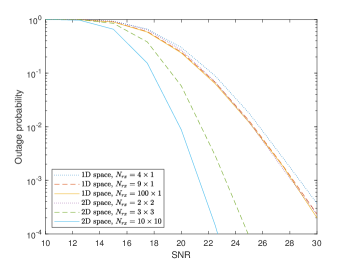
Figure 2: Outage probability of FAS versus SNR for different number of ports and dimensional space, with $q=7{\rm bps/Hz}$.

(a)

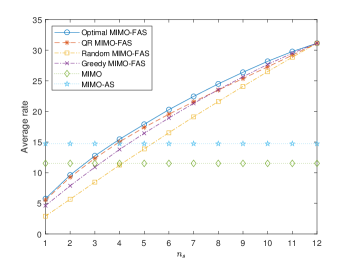
(b)

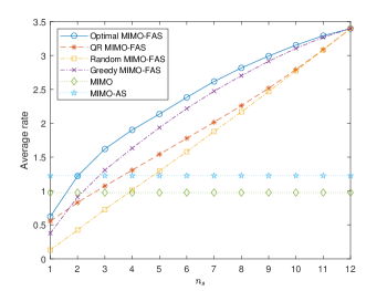
(c)

Figure 3: Average rates of the benchmarking schemes for different values of $n_{s}$: a) ${\rm{SNR}=30}$dB; b) ${\rm{SNR}=10}$dB; c) ${\rm{SNR}=-10}$dB.

To highlight the superiority of 2D space, we first consider a simplified scenario where there is only a single fluid antenna at the receiver. Fig. 2 shows the outage probability of FAS versus SNR for various number of ports and dimensional space. Here, the outage probability is obtained using (46) by replacing $R_{{\rm sys}}\left({\rm SNR}\right)$ with $R_{{\rm QR}}\left({\rm SNR}\right)$. Given the same number of ports, the ports that are distributed in 2D space can achieve a much lower outage probability as compared to the ones that are distributed in 1D space. This improvement can be explained from the fact that a 2D space has an additional dimension for the fluid antenna to move around. Hence, it contains more spatial diversity and yields a lower outage probability. This suggests that the ports in MIMO-FAS should be designed using the entire 2D space for better performance.

Next in Fig. 3, we study the average rates of the benchmarking schemes for different $n_{s}$ at different SNR. Since the optimal MIMO-FAS is computed using an exhaustive search, we set $N_{s}=12$ where $N_{1}^{s}=3$ and $N_{2}^{s}=4$. Fig. 3(a) illustrates that QR MIMO-FAS achieves a similar average rate as compared to the optimal MIMO-FAS at high SNR. Furthermore, the average rate of QR MIMO-FAS scales like $n_{s}\log{\rm SNR}$ when $n_{s}$ ranges from $1$ to $6$. Nevertheless, it suffers from a diminishing rate gain when $n_{s}$ ranges from $7$ to $12$. Thus, MIMO-FAS is most effective when each active port has the freedom of being at least half a wavelength apart from each other. In addition, the average rate of QR MIMO-FAS outperforms traditional MIMO when the number of active ports or antennas is the same (i.e., $n_{s}=4$). This is because QR MIMO-FAS activates the optimal ports in each realization, which reduces the spatial correlation effect. In Fig. 3(b), we further observe that QR MIMO-FAS provides a higher sum-rate in the medium SNR regime when $n_{s}$ is small while greedy MIMO-FAS yields a better performance when $n_{s}$ is large. Nevertheless, as shown in Fig. 3(c), greedy MIMO-FAS is generally more efficient than QR MIMO-FAS in the low SNR regime. These results suggest that an efficient scheme with low complexity is still required to maximize the rate of MIMO-FAS in the medium and low SNR regimes. Besides, QR MIMO-FAS yields a similar or higher rate than MIMO-AS when the number of active ports or antennas is the same.

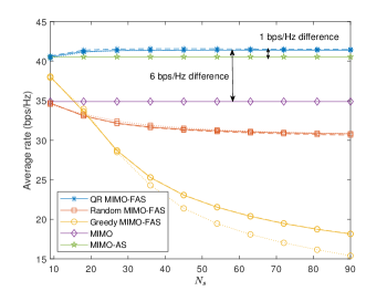
(a)

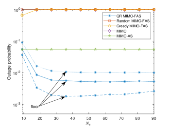
(b)

Figure 4: The performance of the benchmarking schemes for different values of $N_{s}$: (a) average rate; (b) outage probability, with $q=39{\rm bps/Hz}$; (solid) without mutual coupling; (dotted) liquid-based fluid antenna with mutual coupling; (dashed) RF pixel-based fluid antenna with mutual coupling.

Fig. 4 presents the average rates and outage probabilities of the benchmarking schemes for different values of $N_{s}$. In these results, we omit the optimal MIMO-FAS because it is difficult to perform exhaustive search online for large $N_{s}$. On the other hand, since the activated ports can be placed very close to each other, it would be useful to consider the mutual coupling effect and investigate its effect on the performance of MIMO-FAS. In particular, we consider two designs: liquid-based and RF pixel-based fluid antennas. To make a fair comparison between the cases with and without mutual coupling, we assume that $N_{1}^{s}=\left\lfloor\frac{W_{1}^{s}}{0.5}\right\rfloor+1$ and vary $N_{2}^{s}$ accordingly. This means the resolution in one direction is fixed while we change the resolution of FAS in another direction to examine the impact of mutual coupling. The details of the mutual coupling model are given in Appendix III.

As seen in Fig. 4, generally speaking, the performance of QR MIMO-FAS and random MIMO-FAS with mutual coupling are not vastly different from the case without mutual coupling regardless of whether liquid-based or RF pixel-based fluid antenna is considered. This suggests that the active ports can be placed close to each other, typically much less than half a wavelength, and still yield a similar performance. By contrast, the rate performance of greedy MIMO-FAS appears to suffer more from mutual coupling as $N_{s}$ increases. However, greedy MIMO-FAS is not supposed to work well here because the setting is under the high SNR regime.

It is worth pointing out that for RF pixel-based fluid antenna, mutual coupling can exist regardless of whether the pixels are on or off. It is therefore essential to improve the S-matrix via antenna design in order to achieve a good performance. However, the advantage of RF pixel-based fluid antenna is that the mutual coupling matrix is deterministic given $N_{1}^{s}$ and $N_{2}^{s}$ regardless of which pixels are the active ones. Thus, one can directly obtain the optimal port selection, beamforming and power allocation while taking into account of the mutual coupling effect. Moreover, matching networks can be employed directly to further improve the performance of MIMO-FAS but this technique is not considered in our results.

Based on the above observations, we hence focus on the performance of MIMO-FAS without mutual coupling effect. In Fig. 4(a), we see that the average rates of random MIMO-FAS and greedy MIMO-FAS generally decrease as $N_{s}$ increases. This suggests that efficient port selection in MIMO-FAS is essential. Furthermore, the average rate of QR MIMO-FAS is $1{\rm bps/Hz}$ higher than that of MIMO-AS and $6{\rm bps/Hz}$ higher than that of MIMO when $N_{s}$ is large. In Fig. 4(b), the outage probabilities of random MIMO-FAS, Greedy MIMO-FAS and MIMO are near one (i.e., $0.99$) while the outage probability of MIMO-AS is in the order of $10^{-2}$. In contrast, the outage probability of QR MIMO-FAS is much lower (i.e., the order of $10^{-3}$). Nevertheless, the outage probability of QR MIMO-FAS decreases to a floor as $N_{s}$ continues to increase. This limitation is due to the fact that there are approximately $N_{s}^{{}^{\prime}}$ diversity in $\boldsymbol{J}_{s}$ for a fixed $W_{s}$. Therefore, the outage probability of QR MIMO-FAS is limited by $N_{s}^{{}^{\prime}}$ for a fixed $W_{s}$ (see, Table II).

(a)

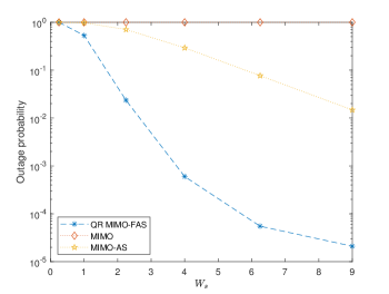
(b)

Figure 5: The performance of QR MIMO-FAS, MIMO and MIMO-AS for different values of $W_{s}$: (a) average rate; (b) outage probability, with $q=42.5$bps/Hz.

To verify this explanation, we further investigate the outage probabilities of QR MIMO-FAS, MIMO and MIMO-AS for different values of $W_{s}$. For brevity, we omit random MIMO-FAS and greedy MIMO-FAS as we now know that these schemes do not provide an effective performance for large $N_{s}$. As seen in Fig. 5(a), the average rates of QR MIMO-FAS, MIMO and MIMO-AS increase and then plateau. Nevertheless, as shown in Fig. 5(b), the outage probabilities of QR MIMO-FAS decrease without bound as $W_{s}$ increases if $N_{s}$ is sufficiently large. By analyzing Table II, we can observe that although $N_{s}$ remains fixed, $N_{s}^{{}^{\prime}}$ generally increases if $W_{s}$ is increased. In contrast, the outage probability of MIMO is always near to being one since the diversity gain of MIMO remains the same even if $W_{s}$ is increased. On the other hand, the outage probability of MIMO-AS decreases at a slower rate due to the lower resolution (i.e., the number of antennas is less than the number of ports in the given space). Overall, Figs. 4 and 5 suggest that the value of $N_{s}$ be determined by $W_{s}$.

From the above results, one might be amazed with the rate improvement of QR MIMO-FAS. Nevertheless, we highlight that the superiority of QR MIMO-FAS lies in the diversity gain. In particular, QR MIMO-FAS can reduce its outage probability to a much lower value than MIMO and MIMO-AS if $q$ is low (e.g., $q<n_{\min}\log{\rm SNR}$). To examine this phenomenon more closely, Fig. 6 illustrates the outage probabilities of QR MIMO-FAS, MIMO and MIMO-AS for different $q$. Within $6{\rm bits/Hz}$, we see that the outage probability of QR MIMO-FAS reduces at a steeper rate (e.g., from the order of $10^{-1}$ to $10^{-5}$) while the outage probability of MIMO-AS reduces at a slower rate (e.g., from the order of $10^{-1}$ to $10^{-2}$) and the outage probability of MIMO remains roughly the same.

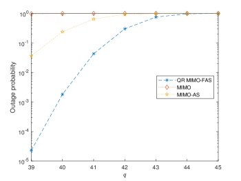
Figure 6: The outage probabilities of QR MIMO-FAS, MIMO and MIMO-AS for different values of $q$.

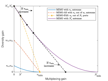
Figure 7: The optimal DMT of MIMO-FAS, MIMO and MIMO-AS.

To understand this at a more fundamental level, we present the DMT of QR MIMO-FAS in Fig. 7. Note that the DMT of QR MIMO-FAS is also the optimal DMT of MIMO-FAS. As shown in Table II, the value of $N_{s}^{{}^{\prime}}$ depends on $W_{s}$ as long as $N_{s}\geq N_{s}^{{}^{\prime}}$. In Fig. 7, it can be seen that the diversity gain of MIMO-FAS is much superior than that of an $n_{rx}\times n_{tx}$ MIMO system for a fixed $r$. For example, the maximum diversity of $4\times 4$ MIMO is $16$ as $r\rightarrow 0$. This is because the optimal DMT of a traditional $n_{rx}\times n_{tx}$ MIMO system is a piecewise linear function connecting the point $\left(r,\left(n_{rx}-r\right)\left(n_{tx}-r\right)\right)$[24]. Meanwhile, the maximum diversity of MIMO-AS is limited by $w_{rx}w_{tx}$. For instance, if $W_{s}=1\lambda^{2}$, the maximum diversity of MIMO-AS is $81$. In contrast, the maximum diversity gain of MIMO-FAS is approximately $23\times 23=529\gg\left\{81,16\right\}$ if $W_{rx}=W_{tx}=1\lambda^{2}$. Hence, the diversity gain of MIMO-FAS is massive because outage only occurs when all the ports experience deep fades. To obtain the same diversity gain at multiplexing gain $r$ from $0$ to $N^{\prime}$, a traditional $N_{rx}^{{}^{\prime}}\times N_{tx}^{{}^{\prime}}$ MIMO would have been required. However, the downside is that it can only have at most $n_{\min}$ multiplexing gain.

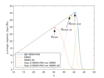
Figure 8: The $q$-outage capacity of MIMO-FAS, MIMO and MIMO-AS.

Finally, we investigate the $q$-outage capacity to showcase the benefits of MIMO-FAS. Fig. 8 presents the $q$-outage capacities of QR MIMO-FAS, MIMO and MIMO-AS as well as the $q$-outage capacity gain of QR MIMO-FAS over MIMO and MIMO-AS. For ease of exposition, the optimal $q^{*}$ of QR MIMO-FAS, MIMO and MIMO-AS are denoted as $q_{{\rm MIMO\text{-}FAS}}^{*}$, $q_{{\rm MIMO}}^{*}$, $q_{{\rm MIMO\text{-}AS}}^{*}$, respectively. As it is seen, the outage capacities of the schemes increase up to $q^{*}$ and decrease thereafter. To the left side of $q^{*}$, the capacity is limited by $q$ (i.e., rate) since $\bar{P}_{{\rm sys}}^{{\rm out}}\left({\rm SNR},q\right)$ is small. To the right side of $q^{*}$, the capacity is limited by the outage probability because $\bar{P}_{{\rm sys}}^{{\rm out}}\left({\rm SNR},q\right)$ is large. Since MIMO provides limited diversity gain and MIMO-AS has a limited number of antennas within a given space, both schemes fail to achieve certain $q$-outage capacity achievable by QR MIMO-FAS. This suggests that MIMO-FAS can reliably deliver a much higher rate than traditional MIMO and MIMO-AS systems.

VI Conclusions

In this paper, we analyzed the performance limits of MIMO-FAS. To this end, we developed a system model for MIMO-FAS where a 2D fluid antenna surface was used at both ends, while taking into account of the spatial correlation of the ports. We then proposed a suboptimal scheme to maximize the rate of MIMO-FAS at high SNR via joint port selection, beamforming and power allocation, namely QR MIMO-FAS. One key contribution was the derivation of the outer bound of the DMT for MIMO-FAS. Through the outer bound and the proposed scheme, we then obtained the optimal DMT of MIMO-FAS which revealed the fundamental limits of MIMO-FAS. Extensive results were presented, illustrating that QR MIMO-FAS achieved a similar rate as compared to the optimal MIMO-FAS in the high SNR regime. By fixing other MIMO-FAS parameters, we found that the average rate and outage probability of QR MIMO-FAS approached to a limit as $N_{s}$ increased. Likewise, the average rate of QR MIMO-FAS improved up to a certain level as $W_{s}$ increased. Nevertheless, the outage probability of QR MIMO-FAS decreased without bound as $W_{s}$ increased. For the same multiplexing gain, we also showed that MIMO-FAS achieved massive diversity gain as compared to the traditional MIMO and MIMO-AS systems. Motivated by this, we further illustrated that MIMO-FAS could reliably deliver a much higher rate than the traditional MIMO and MIMO-AS systems in terms of $q$-outage capacity that jointly considered both rate and outage probability.

Appendix I: Spatial Correlation of 2D Fluid Antenna Surface over 3D Scattering Environment

Without loss of generality, let us refer to the position of the ($n_{1},n_{2}$)-port as $\boldsymbol{n}_{l_{s}}=\left[0,\frac{n_{2}^{s}-1}{N_{2}^{s}-1}W_{2}^{s},\frac{n_{1}^{s}-1}{N_{1}^{s}-1}W_{1}^{s}\right]{}^{T}$ where ${\rm{map}}\left(n_{1},n_{2}\right)=l_{s}$ and $\lambda$ is the wavelength. Suppose a plane wave impinges on the fluid antenna surface from azimuth angle $\varphi$ and elevation angle $\theta$. Then, the array response vector can be expressed as [43]

$$\boldsymbol{a}\left(\varphi,\theta\right)=\left[e^{j\frac{2\pi}{\lambda}\boldsymbol{k}\left(\varphi,\theta\right)^{T}\boldsymbol{n}_{1}\lambda},\dots,e^{j\frac{2\pi}{\lambda}\boldsymbol{k}\left(\varphi,\theta\right)^{T}\boldsymbol{n}_{N_{s}}\lambda}\right]^{T},$$ (48)

where

$$\boldsymbol{k}\left(\varphi,\theta\right)=\left[\begin{array}[]{ccc}\cos\left(\theta\right)\cos\left(\varphi\right)&\cos\left(\theta\right)\sin\left(\varphi\right)&\sin\left(\theta\right)\end{array}\right]^{T},$$ (49)

is the normalized wave vector.

Let us denote the spatial correlation matrix as $\boldsymbol{J}_{s}=\mathbb{{E}}\left\{\boldsymbol{a}\left(\varphi,\theta\right)\boldsymbol{a}\left(\varphi,\theta\right)^{H}\right\}$. From (48), we know that the $\left(k_{s},l_{s}\right)$-th entry of $\boldsymbol{J}_{s}$ can be expressed as

$$\left[\boldsymbol{J}_{s}\right]_{k_{s},l_{s}} =\mathbb{{E}}\left\{e^{j\frac{2\pi}{\lambda}\boldsymbol{k}\left(\varphi,\theta\right)^{T}\boldsymbol{n}_{k_{s}}\lambda}e^{-j\frac{2\pi}{\lambda}\boldsymbol{k}\left(\varphi,\theta\right)^{T}\boldsymbol{n}_{l_{s}}\lambda}\right\}$$

$$=\mathbb{{E}}\left\{e^{j2\pi\boldsymbol{k}\left(\varphi,\theta\right)^{T}\left(\boldsymbol{n}_{k_{s}}-\boldsymbol{n}_{l_{s}}\right)}\right\},$$ (50)

where ${\rm{map}}\left(\tilde{n}_{1}^{s},\tilde{n}_{2}^{s}\right)=k_{s}$. Using the Jacobi-Anger plane wave expansion [44], (50) can be rewritten as

$$\left[\boldsymbol{J}_{s}\right]_{k_{s},l_{s}}=4\pi\sum_{m=0}^{\infty}\sum_{n=-m}^{m}\left(-i\right)^{m}\times\\ \alpha_{m}^{n}Y_{m}^{n}\left(\frac{\boldsymbol{n}_{k_{s}}-\boldsymbol{n}_{l_{s}}}{\left\|\boldsymbol{n}_{k_{s}}-\boldsymbol{n}_{l_{s}}\right\|}\right)\times\\ j_{m}\left(2\pi\left\|\boldsymbol{n}_{k_{s}}-\boldsymbol{n}_{l_{s}}\right\|\right),$$ (51)

where $j_{m}\left(.\right)$ is the spherical Bessel function of the first kind, $Y_{m}^{n}\left(\cdot\right)$ is the spherical harmonics, and

$$\alpha_{m}^{n} =\int_{\Omega}f_{\boldsymbol{k}\left(\varphi,\theta\right)}\left(\boldsymbol{k}\right)Y_{m}^{n}\left(\boldsymbol{k}\right)d\Omega\left(\boldsymbol{k}\right),$$ (52)

where $\Omega\left(\boldsymbol{k}\right)$ is a surface element of a unit sphere $\Omega$. For a 3D isotropic scattering environment, we have $f_{\boldsymbol{k}\left(\varphi,\theta\right)}\left(\boldsymbol{k}\right)=\frac{1}{4\pi}$ and thus (52) reduces to

$$\alpha_{m}^{n}=\frac{1}{4\pi}\int_{\Omega}Y_{m}^{n}\left(\boldsymbol{k}\right)d\Omega\left(\boldsymbol{k}\right).$$ (53)

Using the fact that

$$Y_{m}^{n}\left(\frac{\boldsymbol{n}_{k_{s}}-\boldsymbol{n}_{l_{s}}}{\left\|\boldsymbol{n}_{k_{s}}-\boldsymbol{n}_{l_{s}}\right\|}\right)=\frac{1}{\sqrt{4\pi}}\quad{\rm{if}}\leavevmode\nobreak\ n=m=0,$$ (54)

and

$$\int_{\Omega}Y_{m}^{n}\left(\tilde{\boldsymbol{k}}\right)d\Omega\left(\tilde{\boldsymbol{k}}\right)=\begin{cases}\sqrt{4\pi}&{\rm{if}}\leavevmode\nobreak\ n=m=0,\\ 0&{\rm{otherwise}},\end{cases}$$ (55)

(51) can be rewritten as

$$\left[\boldsymbol{J}_{s}\right]_{k_{s},l_{s}}=j_{0}\left(2\pi\left\|\boldsymbol{n}_{k_{s}}-\boldsymbol{n}_{l_{s}}\right\|\right),$$ (56)

which gives (1). Note that (1) conforms with [45, 46, 47] since $j_{0}\left(c\right)=\frac{\sin c}{c}.$ In addition, (1) can be reduced to a 1D fluid antenna with 2D scattering environment by setting $N_{1}^{s}=1$ and $\frac{0}{0}\triangleq 0$ and replacing $j_{0}\left(\cdot\right)$ by $J_{0}\left(\cdot\right)$ where $J_{0}\left(\cdot\right)$ is the Bessel function of the first kind [9].

Appendix II: Generalization to Other Spatial Correlation Models

Without loss of generality, let us consider a 1D fluid antenna since a similar argument can be made for a 2D fluid antenna surface. To begin with, let us denote $\boldsymbol{J}$ as the $N\times N$ spatial correlation matrix. Suppose that $W\gg 0$, and the spatial correlation between the $k$-th port and the $l$-th port is $J_{k,l}=f\left(k,l,N\right)$ where the spatial correlation function $f$ satisfies two conditions: i) $\lim_{N\rightarrow\infty}f\left(k,k\pm 1,N\right)=1$ and ii) there are some $\exists l\neq k$ such that $f\left(k,l,N\right)\neq 1$. The first condition implies that the $(k\pm 1)$-th row/column of $\boldsymbol{J}$ can be removed from $\boldsymbol{J}$ since the $(k\pm 1)$-th row/column of $\boldsymbol{J}$ is always identical to the $k$-th row/column of $\boldsymbol{J}$ in the limit. The second condition implies that there exist some $l$-th port whose $l$-th row/column must be retained in $\boldsymbol{J}$ since its spatial correlation is completely distinct from the $k$-th port. If $f$ satisfies these two conditions, then there must exist a minimal spacing $c$ between the $k$-th and $l$-th ports such that their spatial correlation is distinct. Using the fact that $W$ is finite, it is clear that there are at most $\bar{N}$ non-identical ports since conditions (i) and (ii) hold. In particular, $\bar{N}$ must be finite because $W\geq\bar{N}c>0$. As a result, $\boldsymbol{J}$ can be rewritten as a symmetric $\bar{N}\times\bar{N}$ finite size matrix. Let us denote $N^{{}^{\prime}}$ as the full rank of the symmetric $\bar{N}\times\bar{N}$ matrix where $N^{{}^{\prime}}\leq\bar{N}$. Then, we can further reduce the symmetric $\bar{N}\times\bar{N}$ matrix to a full rank symmetric $N^{{}^{\prime}}\times N^{{}^{\prime}}$ submatrix $\boldsymbol{J}_{{\rm red}}$ by removing the $(\bar{N}-N^{{}^{\prime}})$ dependent rows and columns. Consequently, $\boldsymbol{J}$ can be represented by $\boldsymbol{J}_{{\rm red}}$ which is a full rank symmetric $N^{{}^{\prime}}\times N^{{}^{\prime}}$ finite-size matrix.

Appendix III: The Effect of Mutual Coupling

In liquid-based fluid antenna, mutual coupling only occurs between the active ports. Thus, the MIMO-FAS channel with mutual coupling effect can be modeled as [48]

$$\boldsymbol{\bar{H}}_{mc}=\boldsymbol{Z}_{mc}^{rx,l}\boldsymbol{\bar{H}}\boldsymbol{Z}_{mc}^{tx,l},$$ (57)

where $\boldsymbol{Z}_{mc}^{rx,l}$ and $\boldsymbol{Z}_{mc}^{tx,l}$ are the mutual coupling matrices which can be pre-computed offline given the antenna technologies used. The mutual coupling matrix is given as

$$\boldsymbol{Z}_{mc}^{s,l}=\left(Z_{A}+Z_{L}\right)\left(\boldsymbol{Z}_{s}^{l}+Z_{L}\boldsymbol{I}\right)^{-1},s\in\left\{rx,tx\right\},$$ (58)

where $Z_{A}$, $Z_{L}$ and $\boldsymbol{Z}_{s}^{l}$ are the antenna impedance, load impedance and mutual impedance matrix of the active ports, respectively. To compute $\boldsymbol{Z}_{s}^{l}$, we assume that each active port is a dipole element with a length of $0.5\lambda$ and a width of $0.001\lambda$. Consequently, $Z_{A}=73.08+42.21j$ and $Z_{L}=Z_{A}^{*}$. Due to the dipole’s physical constraint, we fix $N_{1}^{s}=\left\lfloor\frac{W_{1}^{s}}{0.5}\right\rfloor+1$ and vary $N_{2}^{s}$ accordingly. If all the active ports are far from each other, we have $\boldsymbol{Z}_{mc}^{s}\approx\boldsymbol{I}$. Given (57), SVD and waterfilling power allocation are then performed. It is worth highlighting that this model is a conservative one because the mutual coupling effect is not considered when optimizing $A_{tx}$ and $A_{rx}$. In fact, the performance of MIMO-FAS can be further improved when considering the mutual coupling effect and allowing the optimal active ports to be freely located within the given surface.

In RF pixel-based fluid antenna, mutual coupling can exist regardless of whether the pixels are on or off. Thus, in practice, it is important to improve the S-matrix via antenna design. To a coarse approximation, the S-matrix is modeled as

$$\boldsymbol{S}_{mc}^{s}=\left[\begin{array}[]{cccc}\alpha_{\text{rl}}S_{1,1}^{s}&\alpha_{\text{iso}}S_{1,2}^{s}&\cdots&\alpha_{\text{iso}}S_{1,N_{s}}^{s}\\ \alpha_{\text{iso}}S_{2,1}^{s}&\alpha_{\text{rl}}S_{2,2}^{s}&&\vdots\\ \vdots&&\ddots\\ \alpha_{\text{iso}}S_{N_{s},1}^{s}&\cdots&&\alpha_{\text{rl}}S_{N_{s},N_{s}}^{s}\end{array}\right],$$ (59)

where $\alpha_{\text{rl}}$ and $\alpha_{\text{iso}}$ determine the improvement level of the return loss and isolation, respectively, while $S_{k_{s},l_{s}}^{s}$ is the S-parameter between the $k_{s}$-th and $l_{s}$-th ports. In this paper, we assume that the return loss and isolation levels are $-15$dB and $30$dB, respectively, which are typical values that can be achieved using state-of-the-art technologies [49]. Given (59), the mutual impedance matrix of the RF pixel-based fluid antenna can be computed as

$$\boldsymbol{Z}_{s}^{p}=z_{0}\left(\boldsymbol{I}+\boldsymbol{S}_{mc}^{s}\right)\left(\boldsymbol{I}-\boldsymbol{S}_{mc}^{s}\right)^{-1},$$ (60)

where $z_{0}=50\Omega$ is the reference impedance. Similar to (58), the mutual coupling matrix is given as

$$\boldsymbol{Z}_{mc}^{s,p}=\left(Z_{A}+Z_{L}\right)\left(\boldsymbol{Z}_{s}^{p}+Z_{L}\boldsymbol{I}\right)^{-1},s\in\left\{rx,tx\right\}.$$ (61)

Similar to (57), the MIMO-FAS channel with mutual coupling effect is modeled as

$$\boldsymbol{H}_{mc}=\boldsymbol{Z}_{mc}^{rx,p}\boldsymbol{H}\boldsymbol{Z}_{mc}^{tx,p}.$$ (62)

In contrast to (57) and (58), it is worth noting that (61) and (62) are $N_{s}\times N_{s}$ matrices. Given (62), the port selections, beamforming and power allocation can be performed by different schemes. Note that matching networks can be employed to further improve the performance of MIMO-FAS [50].

References

- [1] F. Tariq et al., “A speculative study on 6G,” IEEE Wireless Commun., vol. 27, no. 4, pp. 118–125, Aug. 2020.
- [2] A. Shojaeifard et al., “MIMO evolution beyond 5G through reconfigurable intelligent surfaces and fluid antenna systems,” Proc. IEEE, vol. 110, no. 9, pp. 1244–1265, 2022.
- [3] K. K. Wong, K. F. Tong, Y. Shen, Y. Chen, and Y. Zhang, “Bruce Lee-inspired fluid antenna system: Six research topics and the potentials for 6G,” Frontiers in Commun. and Netw., section Wireless Commun., 3:853416, Mar. 2022.
- [4] Y. Huang, L. Xing, C. Song, S. Wang and F. Elhouni, “Liquid antennas: Past, present and future,” IEEE Open J. Antennas & Propag., vol. 2, pp. 473–487, 2021.
- [5] A. Grau Besoli and F. De Flaviis, “A multifunctional reconfigurable pixeled antenna using MEMS technology on printed circuit board,” IEEE Trans. Antennas & Propag., vol. 59, no. 12, pp. 4413–4424, Dec. 2011.
- [6] S. Song and R. D. Murch, “An efficient approach for optimizing frequency reconfigurable pixel antennas using genetic algorithms,” IEEE Trans. Antennas & Propag., vol. 62, no. 2, pp. 609–620, Feb. 2014.
- [7] T. Ismail and M. Dawoud, “Null steering in phased arrays by controlling the elements positions,” IEEE Trans. Antennas & Propag., vol. 39, no. 11, pp. 1561–1566, Nov. 1991.
- [8] S. Basbug, “Design and synthesis of antenna array with movable elements along semicircular paths,” IEEE Antennas Wireless Propag. Lett., vol. 16, pp. 3059–3062, Oct. 2017.
- [9] K. K. Wong, A. Shojaeifard, K. F. Tong, and Y. Zhang, “Fluid antenna systems,” IEEE Trans. Wireless Commun., vol. 20, no. 3, pp. 1950–1962, Mar. 2021.
- [10] K. K. Wong, A. Shojaeifard, K. F. Tong, and Y. Zhang, “Performance limits of fluid antenna systems,” IEEE Commun. Lett., vol. 24, no. 11, pp. 2469–2472, Nov. 2020.
- [11] P. Mukherjee, C. Psomas and I. Krikidis, “On the level crossing rate of fluid antenna systems,” in Proc. IEEE Int. Workshop Signal Process. Advances Wireless Commun. (SPAWC), 4-6 Jul. 2022, Oulu, Finland.
- [12] Z. Chai, K. K. Wong, K. F. Tong, Y. Chen, and Y. Zhang, “Port selection for fluid antenna systems,” IEEE Commun. Lett., vol. 26, no. 5, pp. 1180–1184, May 2022.
- [13] L. Tlebaldiyeva, G. Nauryzbayev, S. Arzykulov, A. Eltawil, and T. Tsiftsis, “Enhancing QoS through fluid antenna systems over correlated Nakagami- fading channels,” in Proc. IEEE Wireless Commun. & Netw. Conf. (WCNC), pp. 78–83, 10-13 Apr. 2022, Austin, TX, USA.
- [14] L. Tlebaldiyeva, S. Arzykulov, K. M. Rabie, X. Li, and G. Nauryzbayev, “Outage performance of fluid antenna system (FAS)-aided Terahertz communication networks,” in Proc. IEEE Int. Conf. Commun. (ICC), 28 May-1 Jun. 2023, Rome, Italy.
- [15] M. Khammassi, A. Kammoun and M.-S. Alouini, “A new analytical approximation of the fluid antenna system channel,” IEEE Trans. Wireless Commun., early access DOI:10.1109/TWC.2023.3266411.
- [16] W. K. New, K. K. Wong, H. Xu, K. F. Tong and C.-B. Chae, “Fluid antenna system: New insights on outage probability and diversity gain,” IEEE Trans. Wireless Commun., early access, DOI:10.1109/TWC.2023.3276245.
- [17] C. Skouroumounis and I. Krikidis, “Fluid antenna with linear MMSE channel estimation for large-scale cellular networks,” IEEE Trans. Commun., vol. 71, no. 2, pp. 1112–1125, Feb. 2023.
- [18] L. Zhu, W. Ma, B. Ning, and R. Zhang, “Movable-antenna enhanced multiuser communication via antenna position optimization,” [Online] arXiv preprint arXiv:2302.06978, 2023.
- [19] K. K. Wong, and K. F. Tong, “Fluid antenna multiple access,” IEEE Trans. Wireless Commun., vol. 21, no. 7, pp. 4801–4815, Jul. 2022.
- [20] N. Waqar, K. K. Wong, K. F. Tong, A. Sharples, and Y. Zhang, “Deep learning enabled slow fluid antenna multiple access,” IEEE Commun. Letters, vol. 27, no. 3, pp. 861–865, Mar. 2023.
- [21] K. K. Wong, K. F. Tong, Y. Chen, and Y. Zhang, “Fast fluid antenna multiple access enabling massive connectivity,” IEEE Commun. Lett., vol. 27, no. 2, pp. 711–715, Feb. 2023.
- [22] H. Xu, K. K. Wong, W. K. New, and K. F. Tong, “On the outage probability for two-user fluid antenna multiple access,” in Proc. IEEE Int. Conf. Commun. (ICC), 28 May-1 Jun. 2023, Rome, Italy.
- [23] W. Ma, L. Zhu and R. Zhang, “MIMO capacity characterization for movable antenna systems,” IEEE Trans. Wireless Commun., early access, DOI:10.1109/TWC.2023.3307696.
- [24] L. Zheng and D. Tse, “Diversity and multiplexing: A fundamental tradeoff in multiple-antenna channels,” IEEE Trans. Inform. Theory, vol. 49, no. 5, pp. 1073–1096, May 2003.
- [25] K. K. Wong, K. F. Tong, and C. B. Chae, “Fluid antenna system-Part II: Research opportunities,” IEEE Commun. Lett., early access, DOI:10.1109/LCOMM.2023.3284318.
- [26] S. Sanayei and A. Nosratinia, “Antenna selection in MIMO systems,” IEEE Commun. Mag., vol. 42, no. 10, pp. 68–73, Oct. 2004.
- [27] A. Goldsmith, S. Jafar, N. Jindal, and S. Vishwanath, “Capacity limits of MIMO channels,” IEEE J. Select. Areas Commun., vol. 21, no. 5, pp. 684–702, Jun. 2003.
- [28] N. Iqbal, C. Schneider, and R. S. Thoma, “A fast and optimal deterministic algorithm for NP-Hard antenna selection problem,” in Proc. IEEE Int. Sym. Pers., Indoor, Mobile Radio Commun. (PIMRC), pp. 895–899, 30 Aug-2 Sep. 2015, Hong Kong, China.
- [29] A. Civril and M. Magdon-Ismail, “On selecting a maximum volume sub-matrix of a matrix and related problems,” Theoretical Comp. Sci., vol. 410, no. 47, pp. 4801–4811, 2009.
- [30] M. Gu and S. C. Eisenstat, “Efficient algorithms for computing a strong rank-revealing QR factorization,” SIAM J. Sci. Comp., vol. 17, no. 4, pp. 848–869, 1996.
- [31] W. Ford, Numerical linear algebra with applications: Using MATLAB, Academic Press, 2014.
- [32] N. Prasad and M. K. Varanasi, “Outage theorems for MIMO block-fading channels,” IEEE Trans. Inform. Theory, vol. 52, no. 12, pp. 5284–5296, Dec. 2006.
- [33] Z. Wang and G. Giannakis, “A simple and general parameterization quantifying performance in fading channels,” IEEE Trans. Commun., vol. 51, no. 8, pp. 1389–1398, Aug. 2003.
- [34] L. Zhao, W. Mo, Y. Ma, and Z. Wang, “Diversity and multiplexing tradeoff in general fading channels,” IEEE Trans. Inform. Theory, vol. 53, no. 4, pp. 1549–1557, Apr. 2007.
- [35] Y. Jiang and M. K. Varanasi, “The RF-chain limited MIMO system- part I: Optimum diversity-multiplexing tradeoff,” IEEE Trans. Wireless Commun., vol. 8, no. 10, pp. 5238–5247, Oct. 2009.
- [36] S.-G. Hwang, “Cauchy’s interlace theorem for eigenvalues of Hermitian matrices,” The American Math. Monthly, vol. 111, no. 2, pp. 157–159, 2004.
- [37] H. Moon, “Waterfilling power allocation at high SNR regimes,” IEEE Trans. Commun., vol. 59, no. 3, pp. 708–715, Mar. 2011.
- [38] A. Ghaderipoor, C. Tellambura, and A. Paulraj, “On the application of character expansions for MIMO capacity analysis,” IEEE Trans. Inform. Theory, vol. 58, no. 5, pp. 2950–2962, May 2012.
- [39] S. H. Simon, A. L. Moustakas, and L. Marinelli, “Capacity and character expansions: Moment-generating function and other exact results for MIMO correlated channels,” IEEE Trans. Inform. Theory, vol. 52, no. 12, pp. 5336–5351, Dec. 2006.
- [40] R. G. Gallager, Principles of digital communication, Cambridge University Press Cambridge, UK, vol. 1, 2008.
- [41] L. Zheng and D. Tse, “Communication on the Grassmann manifold: A geometric approach to the noncoherent multiple-antenna channel,” IEEE Trans. Inform. Theory, vol. 48, no. 2, pp. 359–383, Feb. 2002.
- [42] P. C. Hansen, “The truncated SVD as a method for regularization,” BIT Numerical Math., vol. 27, pp. 534–553, 1987.
- [43] E. Bjornson, J. Hoydis, L. Sanguinetti, Massive MIMO networks: Spectral, energy, and hardware efficiency, vol. 11. Now Foundations and Trends, 2017.
- [44] R. Mehrem, “The plane wave expansion, infinite integrals and identities involving spherical Bessel functions,” Appl. Math. & Comp., vol. 217, no. 12, pp. 5360–5365, 2011.
- [45] R. K. Cook, R. Waterhouse, R. Berendt, S. Edelman, and M. Thompson Jr, “Measurement of correlation coefficients in reverberant sound fields,” J. Acoustical Society of America, vol. 27, no. 6, pp. 1072–1077, 1955.
- [46] R. W. Heath Jr and A. Lozano, Foundations of MIMO communication, Cambridge University Press, 2018.
- [47] E. Bjornson and L. Sanguinetti, “Rayleigh fading modeling and channel hardening for reconfigurable intelligent surfaces,” IEEE Wireless Commun. Lett., vol. 10, no. 4, pp. 830–834, Apr. 2021.
- [48] C. T. Neil et al., “On the performance of spatially correlated large antenna arrays for millimeter-wave frequencies,” IEEE Trans. Antennas & Propag., vol. 66, no. 1, pp. 132–148, Jan. 2018.
- [49] A. C. K. Mak, C. R. Rowell and R. D. Murch, “Isolation enhancement between two closely packed antennas,” IEEE Trans. Antennas & Propag., vol. 56, no. 11, pp. 3411–3419, Nov. 2008.
- [50] J. W. Wallace and M. A. Jensen, “Mutual coupling in MIMO wireless systems: A rigorous network theory analysis,” IEEE Trans. Wireless Commun., vol. 3, no. 4, pp. 1317–1325, Jul. 2004.