Neural Operator Learning for Long-Time Integration in Dynamical Systems with Recurrent Neural Networks

Abstract

Deep neural networks are an attractive alternative for simulating complex dynamical systems, as in comparison to traditional scientific computing methods, they offer reduced computational costs during inference and can be trained directly from observational data. Existing methods, however, cannot extrapolate accurately and are prone to error accumulation in long-time integration. Herein, we address this issue by combining neural operators with recurrent neural networks to construct a novel and effective architecture, resulting in superior accuracy compared to the state-of-the-art. The new hybrid model is based on operator learning while offering a recurrent structure to capture temporal dependencies. The integrated framework is shown to stabilize the solution and reduce error accumulation for both interpolation and extrapolation of the Korteweg-de Vries equation.

1 Introduction

Dynamical systems modelling is formally concerned with the analysis, forecasting, and understanding of the behavior of ordinary or partial differential equation (ODE/PDE) systems or similar iterative mappings that represent the evolution of a system’s state. Modern machine learning methods have opened up a new area for building fast emulators for solving parametric ODEs and PDEs. One class of such frameworks are neural operators, which have been gaining popularity as surrogate models for dynamical systems in recent years (Lu et al., 2021; Goswami et al., 2022c, b). While previous research on neural architectures has primarily focused on learning mappings between finite-dimensional Euclidean spaces (Raissi et al., 2019; Samaniego et al., 2020), neural operators learn mappings between infinite-dimensional Banach spaces (Goswami et al., 2022a).

The two popular neural operators which have shown promising results so far are the deep operator network (DeepONet) (Lu et al., 2021) introduced in 2019 and the Fourier Neural operator (FNO) (Li et al., 2020) introduced in 2020. Both operator networks have been applied to solving complex problems for real-world applications in diverse scientific domains, including medicine (Goswami et al., 2022c), physics (Lin et al., 2021; Wen et al., 2022), climate (Kissas et al., 2022; Bora et al., 2023; Pathak et al., 2022) and materials science (Goswami et al., 2022d; You et al., 2022; Rashid et al., 2022). Regardless of the impressive results presented in these works, the problem of approximating system’s behavior over a long-time horizon employing neural operators remains underexplored (Goswami et al., 2023; Wang & Perdikaris, 2023).

To address the issues of operator learning over a long-time horizon, some recent works suggest employing physics-informed DeepONets (Wang & Perdikaris, 2023), using transfer learning and later fine-tuning the pre-trained DeepONet with sparse measurements in the extrapolated zone or with a PDE loss (Zhu et al., 2022), and a hybrid inference approach, integrating neural operators with high-fidelity solvers (Oommen et al., 2022). These approaches, however, require either the knowledge of the underlying PDE or sparse labels in extrapolation.

In this work, we introduce a new framework to handle the challenges of long-time integration. The framework employs a neural operator that learns the system’s state representation at any timestep and a recurrent neural network (RNN) that is placed after the architecture of the neural operator to learn temporal dependencies between the states. This extension of a neural operator can help increase the forecast accuracy over a long-time prediction horizon, since RNNs preserve a hidden state that carries information from the previous timesteps forward, thus enabling the model to capture and utilize temporal dependencies.

We demonstrate the performance of the proposed framework on the non-linear Korteweg-de Vries (KdV) equation and observe a reduction in the error accumulation over time, leading to a more accurate and stable prediction. In our tests, we employ three RNN architectures: standard RNN, long short-term memory (LSTM), and gated recurrent units (GRU). Furthermore, we carry out an analysis to show the benefits and challenges of training the two components of the proposed framework separately (in two-step training) and simultaneously. While combining the operator architecture with the recurrent network takes away the property of resolution invariance of the operators, it can be taken advantage of in operator learning when only limited grid data is available. The variations of the framework are tested on interpolation and extrapolation tasks, in both cases resulting in more accurate and stable long-time predictions than their vanilla counterparts.

2 Recurrent networks with neural operators

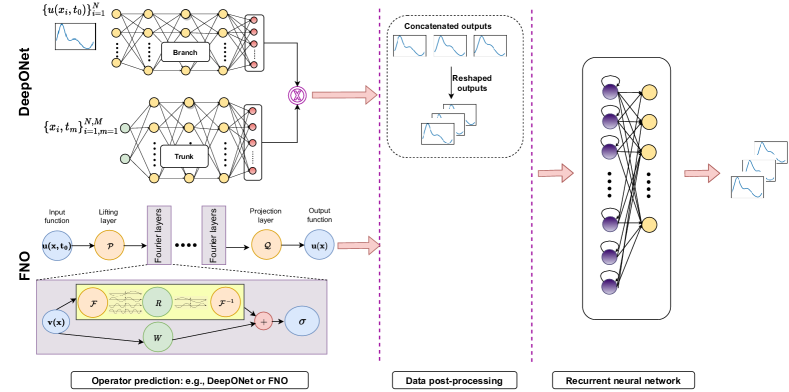
Figure 1: The proposed architecture. The deep neural operator (e.g., DeepONet or FNO) maps the solution operator from the initial condition $u_{t=0}$ to solutions at later timesteps with a fixed time interval $\Delta t$. These solutions are then represented in a temporally sequential manner, i.e., reshaped to [batch_size, nr_timestamps, solution_size], and processed by one of the RNNs. The chosen RNN lifts the dimension to the specified number of neurons and returns all hidden states. The last layer is a fully-connected shallow neural network bringing the embedding to the original size of the solution.

The proposed architecture consists of a deep neural operator followed by a RNN and a feed-forward layer which brings the output back to the dimension of the solution. In this work, we have considered the two most studied neural operators: the deep operator network (DeepONet) and the Fourier neural operator (FNO), combined with one of the three most successful RNNs: the traditional recurrent neural network (non-gated), long short term memory (LSTM), and gated recurrent units (GRU). The architecture is set up such that the outputs of the neural operator are fed as inputs of the RNN. The neural operator learns the solution operator, while the RNN processes the outputs of the neural operator as temporal sequences. A schematic representation of the proposed approach is shown in Figure 1.

The aim of the neural operator is to learn the mapping between two infinite-dimensional functional spaces, where we learn the evolution of a dynamical system from a given initial condition. Such operator mapping can be represented as:

$$\mathcal{N}:u(x,t=0)\rightarrow[u(x,t_{1}),...,u(x,t_{n})],$$

where $n$ is the total number of temporal discretization points that defines the full trajectory and $\mathcal{N}$ is the nonlinear operator that defines the PDE. The RNN is employed to identify the outputs of the operator as a sequence. The work is motivated by the fact that in feed-forward neural networks (including neural operators) all the outputs are independent, which is not true for sequence learning. Recurrent networks address this issue through feedback loops and hidden states which allow for the information to be passed forward and capture the temporal dependencies between the outputs.

2.1 Neural operator learning

Neural operators learn nonlinear mappings between infinite-dimensional functional spaces on bounded domains, providing a unique simulation framework for the real-time prediction of multi-dimensional complex dynamics. Once trained, such models are discretization invariant, which means they share the same network parameters across different parameterizations of the underlying functional data. In this study, we consider the performance of two neural operators, DeepONet proposed in (Lu et al., 2021) and FNO proposed in (Li et al., 2020) with our novel recurrent-networks-integrated neural operator architecture (Figure 1).

FNO: The Fourier Neural Operator is based on Green’s theorem, which involves parameterizing the integral kernel in the Fourier space. The input to the network is elevated to a higher dimension, then passed through several Fourier layers before being projected back to the original dimension with a feed-forward layer. Each Fourier layer involves a forward fast Fourier transform (FFT), followed by a linear transformation of the low-Fourier modes and then an inverse FFT. Finally, the output is added to a weight matrix, and the sum is passed through an activation function to introduce nonlinearity. Different variants of FNO have been proposed based on the pre-decided dimensions to replace the integral kernel with the convolution operator defined in Fourier space. A numerical problem that is $1$D in space and $1$D in time could be handled using either FNO-$2$D, which employs Fourier convolutions through space and time to learn the dynamics directly over multiple timesteps, given an initial condition, or using FNO-$1$D, which performs Fourier convolution in space and uses a recurrent time-marching approach to propagate the solution in time. In this work, we employ FNO-$2$D, since time-marching approaches are known to be prone to error accumulation in long time series prediction.

DeepONet: The deep operator network is based on the universal approximation theorem for operators (Chen & Chen, 1995) and employs two deep neural networks (branch and trunk network) to learn a family of PDEs and provide a discretization-invariant emulator, which allows for fast inference and low generalization error (Lanthaler et al., 2022). The branch network encodes the input function (the initial or boundary conditions, constant or variable coefficients, source terms) at fixed sensor points while the trunk network encodes the information related to the spatio-temporal coordinates of the output function. The output embeddings of the branch and the trunk networks are multiplied element-wise and summed over the neurons in the last layer of the networks (Einstein summation). Once the network is trained, it can be employed to interpolate the solution at any spatial and temporal location within the domain.

2.2 The choice of the recurrent neural network

Feed-forward neural networks lack explicit mechanisms to learn dependencies between outputs, which is a fundamental problem when learning temporal sequences. Recurrent neural networks are an extension over traditional neural networks designed to improve sequence learning by preserving a hidden state which carries information from the previous time steps. During training, this hidden state is updated with the current input and the previous hidden state. Another way of learning temporal sequences is through autoregressive methods, which recursively update the input function using the outputs obtained at the previous time steps. This approach, however, is known to result in high error accumulation in long-term time series forecasting.

Since traditional RNNs are prone to vanishing gradients in long sequences, i.e., the gradients used in training approach zero as they are multiplied with each time step to adjust the weights. Therefore, we also investigate the proposed architecture when combined with GRU and LSTM. GRUs and LSTMs address the problem of vanishing gradients by introducing a set of gates, implemented as Sigmoid functions, that allow or block the flow of long-term information through the network. Since the name RNN can refer to both the whole class of recurrent neural networks, as well as the specific architecture, we further use the term simple RNN when referring to non-gated recurrent architecture and RNN for all types of recurrent neural networks, including simple RNN, GRU, and LSTM.

2.3 Simultaneous vs. two-step training

We distinguish two modes of training the networks in the proposed architecture: simultaneous training, in which at each training step the weights of both networks are updated in a single backward pass, and two-step training, where we first train the neural operator network and then the RNN.

The two-step approach allows to take advantage of the resolution-invariance property of neural operators in the training. While the RNNs require evenly spaced data, the operator alone can be trained in a discretization-invariant manner, e.g., to increase the number of training samples when multi-resolution data is available. The neural operator is trained until its validation error does not change substantially in consecutive epochs and is then used in inference to produce the training data for the RNN. The RNN learns a mapping between the outputs of the neural operator and the ground truth, in a manner equivalent to freezing the weights of the neural operator network and continuing the training. However, this approach can also cause additional error accumulation since the approximation error in the neural operator layers cannot be reduced at the point of training the RNN, which is not the case in the simultaneous training mode.

In the remainder of the paper, we refer to the architectures trained in the simultaneous mode as DON-RNN and FNO-RNN, and as DON+RNN, FNO+RNN, and equivalent to the architectures trained in the two-step mode.

3 Results and discussion

Table 1: E1: Interpolation. Performance of models trained and tested on full trajectories ($t\in[0,5]$).

Two-step training	MAE	RMSE	RSE
DeepONet	0.035	0.105	0.034
DON+RNN	0.026	0.093	0.026
DON+GRU	0.019	0.083	0.021
DON+LSTM	0.019	0.085	0.022
FNO	0.027	0.052	0.008
FNO+RNN	0.020	0.032	0.003
FNO+GRU	0.012	0.020	0.001
FNO+LSTM	0.010	0.018	0.001
Simultaneous training	MAE	RMSE	RSE
DON-RNN	0.020	0.032	0.003
FNO-RNN	0.023	0.036	0.004

Table 2: E2: Extrapolation. Performance of models trained on partial trajectories (50 steps $t\in[0,1.25]$), tested on the full trajectories in a recursive manner ($200$ steps in $t\in[0,5]$), where the output of the last prediction step is the input for the next prediction step).

Two-step training	MAE	RMSE	RSE
DeepONet	0.043	0.131	0.052
DON+RNN	0.046	0.141	0.061
DON+GRU	0.042	0.125	0.047
DON+LSTM	0.041	0.125	0.047
FNO	0.089	0.215	0.141
FNO+RNN	0.064	0.172	0.090
FNO+GRU	0.036	0.112	0.038
FNO+LSTM	0.035	0.100	0.030
Simultaneous training	MAE	RMSE	RSE
DON-RNN	0.039	0.110	0.036
FNO-RNN	0.090	0.243	0.179

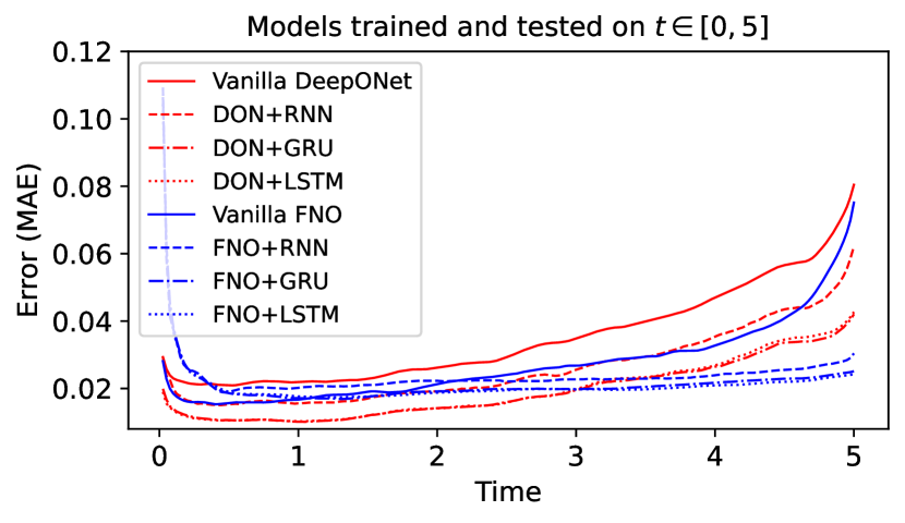
(a) Two-step training.

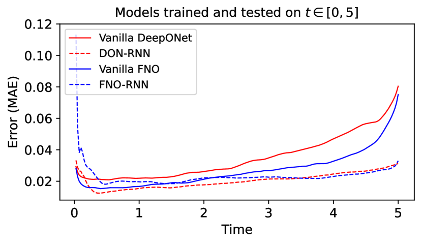
(b) Simultaneous training.

Figure 2: E$1$: Interpolation performance. The models are both trained and tested on full trajectories ($200$ steps in $t\in[0,5]$). The error is given as the MAE over all spatial points $x$ for each time step $t$ on the test data. The enhanced models are compared to vanilla neural operators.

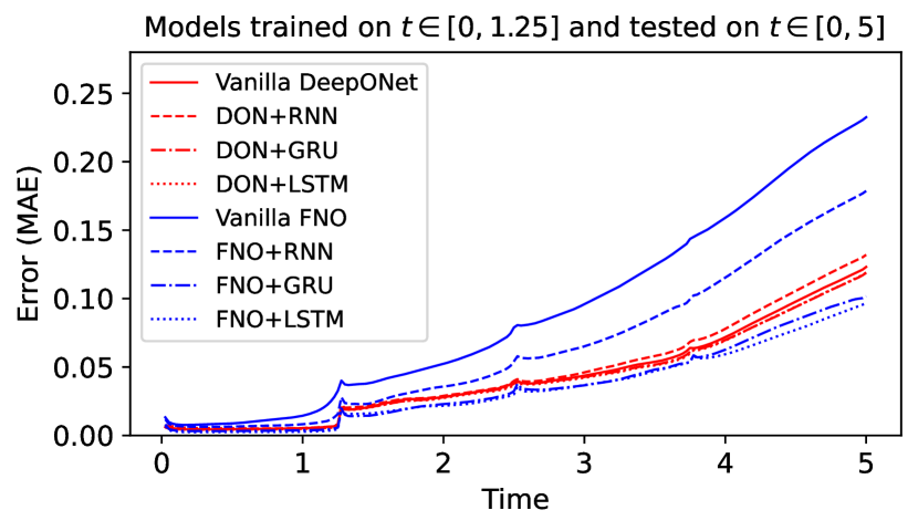
(a) Two-step training.

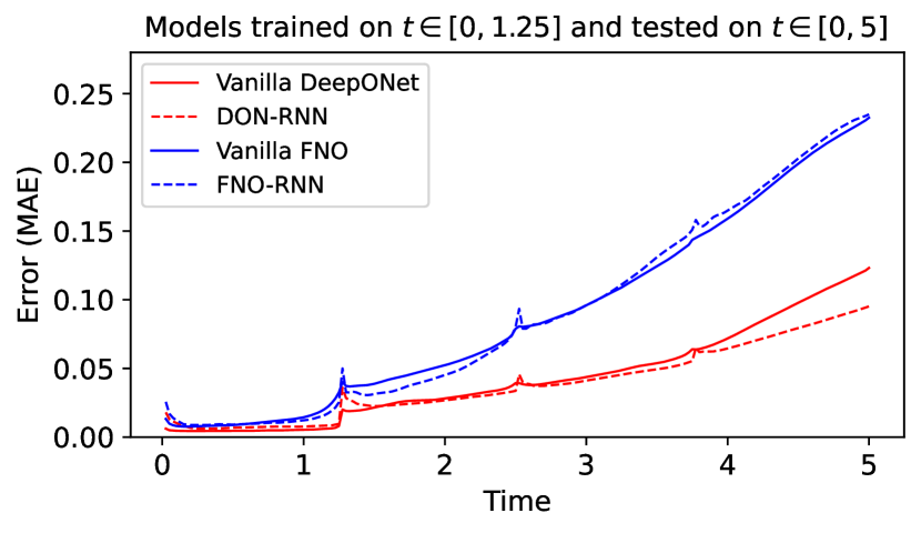
(b) Simultaneous training.

Figure 3: E$2$: Extrapolation performance. The models are trained on partial trajectories ($50$ steps in $t\in[0,1.25]$) and tested on full trajectories ($200$ steps in $t\in[0,5]$). The error is given as the MAE over all spatial points $x$ for each time step $t$ on the test data. The enhanced models are compared to vanilla neural operators.

3.1 Problem statement and data generation

To evaluate the performance of the proposed architecture, we consider the Korteweg-de Vries (KdV) equation defined in Equation 1, which is a nonlinear dispersive PDE that describes the evolution of small-amplitude, long-wavelength system in a variety of physical systems, such as shallow water waves, ion-acoustic waves in plasmas, and certain types of nonlinear optical waves.

$$u_{t}-\eta uu_{x}+\gamma u_{xxx}=0,$$ (1)

where $u$ is the amplitude of the wave, $\eta$ and $\gamma$ are chosen real-valued scalar parameters, $x$ is a spatial and $t$ is the time dimension. The subscripts denote partial derivatives with respect to that variable.

The chosen initial condition, $u(x,0)$ is a sum of two solitons (solitary waves), i.e., $u=u_{1}+u_{2}$. A single soliton is expressed as:

$$\small{u_{i}(x,0)=2k_{i}^{2}\text{sech}^{2}\left(k_{i}((x+\frac{P}{2}-Pd_{i})\%P-\frac{P}{2})\right)^{2},}$$ (2)

where $\mathrm{sech}$ stands for hyperbolic secant ($\frac{1}{\mathrm{cosh}}$), $P$ is the period in space, $\%$ is a modulo operator, $i=\{1,2\}$, $k\in[0.5,1.0]$ and $d\in[0,1]$ are coefficients that determine the height and location of the peak of a soliton, respectively.

To train the recurrent-networks-integrated neural operator, we generated $N=5\small{,}000$ initial conditions, $u(x,t=0)$, and the evolution dynamics was modeled using the midpoint method. The simulation takes place on a $1$D domain $\Omega=[0,10]$ discretized with $50$ uniformly spaced grid points ($\Delta x=0.2$) in the time interval $t=[0,5]$ for $\Delta t=0.025$, thereby discretizing the temporal domain into $201$ points. To form the training data set, we collect solution snapshots $u(x,t)$ at $n_{t}=200$.

The generated labeled dataset with $N$ unique realizations is split into training and testing sets such that the number of training samples, $N_{train}=0.9\times N$ and the number of testing samples, $N_{test}=0.1\times N$. Furthermore, $10$% of the training set is used explicitly for validation during the training process. The detailed architectures of the DeepONet and FNO in this study are discussed in the Appendix B.

To test the proposed framework, we carried out the following two experiments:

• E1: Training and testing on the mapping $\mathcal{N}:u(x,t=0)\rightarrow u(x,t)$, where $t\in[0.025,5]$, where $\mathcal{N}$ denotes the integrated model.

• E2: Training to learn the mapping $\mathcal{N}:u(x,t=0)\rightarrow u(x,t)$, where $t\in[0,1.25]$s, and testing on $t\in[1.25,5]$ by recursively updating the the initial condition.

For each of the experiments, we have considered the two training processes discussed in subsection 2.3, and have carried out an analysis for the combination of two neural operators (DeepONet and FNO) and recurrent networks (simple RNN, LSTM, and GRU). Furthermore, we have investigated the improvement in the accuracy of the proposed framework against the accuracy of vanilla neural operators.

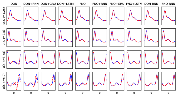
Figure 4: E$1$: Interpolation performance on one representative sample for all models trained on $t\in[0,5]$. The full trajectory $t\in[0.025,5]$ is predicted in one shot. Each subplot shows predictions (red dashed line) and the ground truth (blue solid line) row-wise at $t=\{1.25,2.5,3.75,5\}$ and column-wise for all models: vanilla DeepONet, DeepONet+RNN, GRU, LSTM trained in two steps, vanilla FNO, FNO+RNN, GRU, LSTM trained in two steps, and simultaneously trained DON-RNN and FNO-RNN.

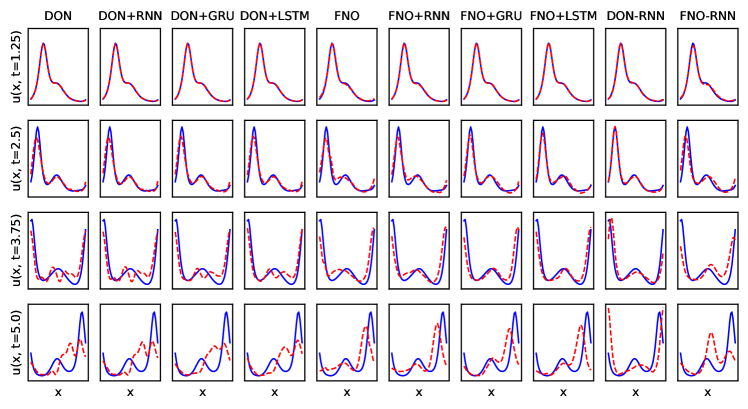
Figure 5: E$2$: Extrapolation performance on one representative sample for all models trained on $t\in[0,1.25]$. The full trajectory $t\in[0.025,5]$ is covered recursively as short-interval one-shot predictions, i.e., as $t=0\rightarrow t\in[0.025,1.25]$, $t=1.25\rightarrow t\in[1.275,2.5]$, up to $t=5$, where the last predicted solution is used as the initial condition for the next one-shot prediction over the interval $\Delta t=1.25$. Each subplot shows predictions (red dashed line) and the ground truth (blue solid line) for the last solution (the next initial condition) row-wise at $t=\{1.25,2.5,3.75,5\}$ and column-wise for all models: vanilla DeepONet, DeepONet+RNN, GRU, LSTM trained in two steps, vanilla FNO, FNO+RNN, GRU, LSTM trained in two steps, and simultaneously trained DON-RNN and FNO-RNN.

3.2 E1: Interpolation performance

The aim of this experiment is to learn the dynamics of the system defined over a time $t\in[0.025,5]$, which is discretized with $200$ temporal points from the given initial condition. The models are trained and tested on complete trajectories ($200$ steps in time $t\in[0.025,5]$). In Table 1, we show the mean absolute error (MAE), root mean square error (RMSE) and the relative squared error (RSE) on the $N_{test}$ test cases for a total of $10$ different architectures. Overall, the integration of recurrent networks with neural operators improves the accuracy and stability of prediction for all architectures. The error accumulation over time for all the architectures is presented in Figure 2.

In particular, for both neural operators, the lowest errors in the two-step training are obtained by the LSTM and GRU extensions (see Table 1). Furthermore, the growth rate of the error is significantly reduced after integrating the recurrent networks with neural operators (see 2(a)). The simultaneous training mode shows an advantage over the two-step training for both operators (see 2(b)) as the accumulated error is drastically reduced, which eventually reduces the slope of the error growth. We report a slight increase in the overall error of the simultaneous training of the RNN extension of the FNO architecture compared to the two-step training as seen in Table 1. However, this increase is due to the high error in the first few time steps (2(b)). A slight increase in error is also observed in the RNN extension of DeepONet when trained simultaneously. Since the high error followed by its decrease in the very few initial timesteps is observed in all trained models, we suspect that the mechanism causing it is independent of the model.

For illustration purposes, the prediction plots for all the architectures are shown for four time snapshots $t=\{1.25,2.5,3.75,5\}$ from a given initial condition in Figure 4. Vanilla DeepONet introduces wiggles to the solution already at time $t=2.5$, and it can be seen that with the RNN extensions, these artifacts become less pronounced, to the point where they disappear completely when the DeepONet is trained simultaneously with a simple RNN. FNO does not seem to suffer from similar instabilities, although it is noticeable that the model does not fit well at the wave peaks in later timesteps. This problem is not visible in the predictions by the extended FNOs.

3.3 E2: Extrapolation performance

This experiment aims to test the performance of the integrated framework for extrapolation. To that end, the models are trained to lean the mapping $\mathcal{N}:u(x,t=0)\rightarrow u(x,t)$, where $t\in[0.025,1.25]$ is discretized to $50$ temporal points. The model is tested to predict the dynamics over time $t\in[0,5]$ for a given initial condition. During testing, the prediction is performed in a recursive manner, where $50$ time steps are predicted in one shot, and in each iteration, the last predicted observation becomes an input (initial condition) for the next $50$ time steps.

The error metrics for all the architectures are presented in Table 2. Similarly to the results obtained in the experiment E$1$, we observe lower error for the RNN extension of the neural operator in all cases, except for the simultaneously trained FNO-RNN architecture (Table 2). Furthermore, gated recurrent networks like GRU and LSTM show advantages over simple RNN. Figure 3 shows that all models suffer from significant error accumulation.

In all cases, the neural operators integrated with recurrent networks trained in a two-step procedure show lower error accumulation over time, especially for GRU and LSTM (3(a)). Significant improvement is observed in the accuracy of FNO integrated with the recurrent networks, where the slope of the error growth is also reduced. However, we observe that in temporal extrapolation, the recurrent integrated architecture of DeepONet performs similarly to the vanilla DeepONet in the first two iterations, and accumulates larger error after the third iteration. For simultaneous training (3(b)), the DON-RNN architecture has lower error and slower growth than the vanilla DeepOnet in the last iteration, regardless of a pronounced error increase at the beginning of each iteration. Furthermore, the FNO-RNN architecture shows similar performance to the vanilla FNO.

To investigate further, we plot the temporal evolution of a representative sample for four time snapshots $t=\{1.25,2.5,3.75,5\}$ in Figure 5. Overall, it is observed that the models struggle to maintain the wave shape in extrapolation. Each row shows the last time step in one iteration of the recursive prediction. While at $t=1.25$ all models fit the data, at the last time step of the second iteration ($t=2.5$) the peaks of the waves are underestimated, with an exception of simultaneous training of the recurrent network and DeepONet. At $t=3.75$ the shape of the wave is significantly perturbed for all models but for the two-step training of FNO with GRU and LSTM and the simultaneous training of DeepOnet with RNN. Finally, at $t=5.0$ the shape remains partially captured for these models, but with an offset in the spatial dimension, while the remaining models have lost all resemblance to the ground truth.

4 Conclusions

While neural methods have been shown to be promising surrogate models to accelerate the simulation of dynamical systems, integrating these systems over long-time horizons still remains an open challenge. Some recent works propose to address this problem by employing physics-informed deep operator networks, transfer learning, or hybrid approaches, however, these methods suffer from their own limitations.

In this work, we have proposed a new approach to tackle long-time horizon prediction, that combines two existing and successful architectures: neural operators and recurrent neural networks. The resulting model shows improvement in terms of accuracy and stability of prediction.

We have illustrated the advantage of this new architecture for long-time integration by comparing it to the vanilla form of two neural operators, DeepONet and FNO, on the Korteweg-de Vries equation, which is a nonlinear equation for modeling shallow water waves.

Our observations from this study can be summarized as follows:

1. The proposed extension of the neural operators reduces the overall error in both interpolation and extrapolation experiments when compared to vanilla models, as well as the error accumulation over the whole trajectory for all models except for the extrapolation on simultaneously trained FNO-RNN (Tables 1 and 2, Figures 2 and 3).

2. The error growth rate is also reduced for most of the models. In the interpolation tests, the accumulated error practically flattens out for all extensions of neural operators, with the exception of the models trained with a DeepONet in the two-step process, where the error is lower, but still shows significant accumulation (Figure 2). In extrapolation, the reduction in the error growth rate is significant for the FNO trained in a two-step process, as well as for the simultaneously trained DON-RNN (3(a)).

3. The proposed architecture is shown to improve the ability of the operator to maintain the shape of the solution, which prevents some of the error propagation in long-time integration (Figures 4, 5). The stability is more pronounced when the components of the integrated framework are trained simultaneously.

Despite the promising results presented here, we must acknowledge that using the RNN-integrated neural operator architecture to solve long-term prediction problems is still in its infancy. Numerous open issues should be taken into account as potential future study topics. It is crucial from a theoretical standpoint to gain a better understanding of how approximation errors impact the stability and precision of the suggested methods. This is a key component in critical applications where accuracy and convergence guarantees are required, where conventional numerical solvers are still the default option at the moment.

5 Acknowledgement

For KM and SRS, this work is based upon the support from the Research Council of Norway under project SFI NorwAI 309834. Furthermore, KM is also supported by the PhD project grant 323338 Stipendiatstilling 17 SINTEF (2021-2023). For SG and GEK, this work was supported by the U.S. Department of Energy, Advanced Scientific Computing Research program, under the Scalable, Efficient and Accelerated Causal Reasoning Operators, Graphs and Spikes for Earth and Embedded Systems (SEA-CROGS) project, DE- SC0023191. Furthermore, the authors would like to acknowledge the computing support provided by the computational resources and services at the Center for Computation and Visualization (CCV), Brown University where all the experiments were carried out.

Appendix A Nomenclature

Table 3: Symbols and abbreviations used in the work.

Symbol	Description
DON, DeepONet	Deep operator network
FNO	Fourier neural operator
GRU	Gated recurrent unit
LSTM	Long short term memory
MAE	Mean absolute error
RNN	Recurrent neural network
RMSE	Root mean squared error
RSE	Relative squared error
R2	R-squared, the coefficient of determination
PDE	Partial differential equation
DON-RNN	Proposed architecture with DON and RNN trained in the simultaneous mode
DON+RNN	Proposed architecture with DON and RNN trained in the two-step mode

Appendix B Neural network architectures

B.1 DeepONet

The vanilla DeepONet is constructed with a branch and trunk network with the same output sizes, which are merged using Einstein summation (Figure 1). The input to the branch network is of the size [batch_size, x_len], the input to the trunk network is of the size [x_len$\times$t_len, 2], and the output of the network after the Einstein summation is [batch_size, x_len$\times$t_len], where batch_size refers to the number of samples in each minibatch, and x_len and t_len, to the sizes of the spatial and temporal dimensions, i.e., the number of discretization points.

Table 4: Branch network. Total nr of parameters is $547,950$.

	Layer	Output shape	Activation	Param
0	Input	(None, 50)	-	$0$
1	Dense	(None, 150)	swish	$7,650$
2	Dense	(None, 250)	swish	$37,750$
3	Dense	(None, 450)	swish	$112,950$
4	Dense	(None, 380)	swish	$171,380$
5	Dense	(None, 320)	swish	$121,920$
6	Dense	(None, 300)	linear	$96,300$

Table 5: Trunk network. Total nr of parameters is $380,750$.

	Layer	Output shape	Activation	Param
0	Input	(None, 2)	-	0
1	Dense	(None, 200)	swish	$600$
2	Dense	(None, 220)	swish	$44,220$
3	Dense	(None, 240)	swish	$53,040$
4	Dense	(None, 250)	swish	$60,250$
5	Dense	(None, 260)	swish	$65,260$
6	Dense	(None, 280)	linear	$73,080$
7	Dense	(None, 300)	linear	$84,300$

The DeepONet is trained in minibatches of 256 samples using the Adam optimizer and learning rate of $1e-4$. For the DeepONet the data is normalized in the following manner: the inputs to the branch network and the outputs of the DeepONet use standard scaling, and the inputs to the trunk network use min-max (Appendix D). The vanilla DeepONet for the full trajectory is trained up to $100,000$ epochs, while the other DeepONet and DeepONet-RNN architectures up to $75,000$ epochs. The models used in inference are the ones at $40,000$ epochs, as no improvement is seen for the longer training.

B.2 Fourier neural operator

A single Fourier layer is constructed with a 2D spectral convolution and a 2D-convolution skip connection.

Table 6: Fourier neural operator architecture for the input of 200 timesteps. Total nr of parameters is $25,345$.

	Layer	Output shape	Activation	Param
0	Input	(None, 200, 50, 1)	-	$0$
1	Dense	(None, 200, 50, 64)	linear	$256$
2	Fourier	(None, 64, 209, 59)	-	$4,160$
3	Fourier	(None, 64, 209, 59)	-	$4,160$
4	Fourier	(None, 64, 209, 59)	-	$4,160$
5	Fourier	(None, 64, 209, 59)	-	$4,160$
6	Dense	(None, 200, 50, 128)	linear	$8,320$
7	Dense	(None, 200, 50, 1)	linear	$129$

The FNO is trained in minibatches of 50 samples using the Adam optimizer, the learning rate of $1e-3$ and a scheduler with a step size of 100. The inputs and outputs of the FNO are not scaled. The vanilla FNOs are trained up to $5000$ epochs, while FNO-RNN up to $2000$ epochs. The models used in inference are the ones at a $1000$ epochs, as no further improvement is seen for longer training.

B.3 RNN extension of neural operators

Table 7: RNN extension for the input of $200$ timesteps. Total nr of parameters is $60,250$.

	Layer	Output shape	Activation	Param
0	Input	(None, 10000)	-	$0$
1	Reshape	(None, 200, 50)	-	$0$
2	RNN	(None, 200, 200)	tanh	$50,200$
3	Dense	(None, 200, 50)	linear	$10,050$

The inputs and outputs in RNN training are normalized using standard scaling if trained in a two-stage mode and in the same manner as the vanilla DeepONet/FNO inputs and outputs when trained simultaneously. The models are trained up to $10,000$ epochs.

When using gated units instead of the simple RNN, the number of parameters is considerably higher. For GRU, Layer #2 has $151,200$ parameters and the whole network has $161,250$ parameters. For LSTM, Layer #2 has $200,800$ parameters and the whole network has $210,850$ parameters.

Appendix C Metrics

In this study, we used several metrics to evaluate the performance of the model such as mean average error, root mean squared error, relative error and R-squared.

C.1 Mean average error

The mean average error (MAE) is expressed as:

$$\text{MAE}=\frac{1}{n}\sum_{i=1}^{n}|y_{i}-\hat{y_{i}}|,$$ (3)

where $n$ is the number of samples, $y_{i}$ is the true value of the $i^{th}$ sample, and $\hat{y_{i}}$ is the predicted value of the $i^{th}$ sample.

C.2 Root mean squared error

The root mean squared error (RMSE) is expressed as:

$$\text{RMSE}=\sqrt{\frac{1}{n}\sum_{i=1}^{n}(y_{i}-\hat{y_{i}})^{2}},$$ (4)

where: $n$ is the number of samples, $y_{i}$ is the true value of the $i^{th}$ sample and $\hat{y_{i}}$ is the predicted value of the $i^{th}$ sample.

C.3 Relative squared error

The relative squared error (RSE) is the total squared error between the predicted values and the ground truth normalized by the total squared error between the ground truth and the mean. The metric is expressed as:

$$\text{RSE}=\frac{\frac{1}{n}\sum_{i=1}^{n}(y_{i}-\hat{y_{i}})^{2}}{\frac{1}{n}\sum_{i=1}^{n}(y_{i}-\bar{y})^{2}}$$ (5)

where $y_{i}$ is the true value of the $i^{th}$ sample, $\hat{y_{i}}$ is the predicted value of the $i^{th}$ sample, and $\bar{y}$ is the mean value of all samples.

Appendix D Data normalization

D.1 Standard scaling

The standard scaling formula is defined as:

$$x^{\prime}=\frac{x-\mu}{\sigma},$$ (6)

where $x^{\prime}$ are the standardized values, $x$ are the original values, $\mu$ is the mean, and $\sigma$ is the standard deviation of $x$.

D.2 Min-max scaling

Min-max scaling, also known as Min-max normalization, scales the data between 0 and 1. It is expressed by the equation:

$$x^{\prime}=\frac{x-x_{min}}{x_{max}-x_{min}},$$ (7)

where $x^{\prime}$ are the normalized values, $x$ are the original values, and $x_{min}$ and $x_{max}$ are the minimal and maximal values of $x$.

References

- Bora et al. (2023) Bora, A., Shukla, K., Zhang, S., Harrop, B., Leung, R., and Karniadakis, G. E. Learning bias corrections for climate models using deep neural operators. arXiv preprint arXiv:2302.03173, 2023.
- Chen & Chen (1995) Chen, T. and Chen, H. Universal approximation to nonlinear operators by neural networks with arbitrary activation functions and its application to dynamical systems. IEEE Transactions on Neural Networks, 6(4):911–917, 1995.
- Goswami et al. (2022a) Goswami, S., Bora, A., Yu, Y., and Karniadakis, G. E. Physics-informed deep neural operators networks. arXiv preprint arXiv:2207.05748, 2022a.
- Goswami et al. (2022b) Goswami, S., Kontolati, K., Shields, M. D., and Karniadakis, G. E. Deep transfer operator learning for partial differential equations under conditional shift. Nature Machine Intelligence, pp. 1–10, 2022b.
- Goswami et al. (2022c) Goswami, S., Li, D. S., Rego, B. V., Latorre, M., Humphrey, J. D., and Karniadakis, G. E. Neural operator learning of heterogeneous mechanobiological insults contributing to aortic aneurysms. Journal of the Royal Society Interface, 19(193):20220410, 2022c.
- Goswami et al. (2022d) Goswami, S., Yin, M., Yu, Y., and Karniadakis, G. E. A physics-informed variational DeepONet for predicting crack path in quasi-brittle materials. Computer Methods in Applied Mechanics and Engineering, 391:114587, 2022d. ISSN 0045-7825.
- Goswami et al. (2023) Goswami, S., Jagtap, A. D., Babaee, H., Susi, B. T., and Karniadakis, G. E. Learning stiff chemical kinetics using extended deep neural operators. arXiv preprint arXiv:2302.12645, 2023.
- Kissas et al. (2022) Kissas, G., Seidman, J. H., Guilhoto, L. F., Preciado, V. M., Pappas, G. J., and Perdikaris, P. Learning operators with coupled attention. Journal of Machine Learning Research, 23(215):1–63, 2022.
- Lanthaler et al. (2022) Lanthaler, S., Mishra, S., and Karniadakis, G. E. Error estimates for DeepONets: A deep learning framework in infinite dimensions. Transactions of Mathematics and Its Applications, 6(1):tnac001, 2022.
- Li et al. (2020) Li, Z., Kovachki, N., Azizzadenesheli, K., Liu, B., Bhattacharya, K., Stuart, A., and Anandkumar, A. Fourier neural operator for parametric partial differential equations, 2020.
- Lin et al. (2021) Lin, C., Li, Z., Lu, L., Cai, S., Maxey, M., and Karniadakis, G. E. Operator learning for predicting multiscale bubble growth dynamics. The Journal of Chemical Physics, 154(10):104118, 2021.
- Lu et al. (2021) Lu, L., Jin, P., Pang, G., Zhang, Z., and Karniadakis, G. E. Learning nonlinear operators via DeepONet based on the universal approximation theorem of operators. Nature Machine Intelligence, 3(3):218–229, mar 2021. doi: 10.1038/s42256-021-00302-5.
- Oommen et al. (2022) Oommen, V., Shukla, K., Goswami, S., Dingreville, R., and Karniadakis, G. E. Learning two-phase microstructure evolution using neural operators and autoencoder architectures. arXiv preprint arXiv:2204.07230, 2022.
- Pathak et al. (2022) Pathak, J., Subramanian, S., Harrington, P., Raja, S., Chattopadhyay, A., Mardani, M., Kurth, T., Hall, D., Li, Z., Azizzadenesheli, K., et al. Fourcastnet: A global data-driven high-resolution weather model using adaptive Fourier neural operators. arXiv preprint arXiv:2202.11214, 2022.
- Raissi et al. (2019) Raissi, M., Perdikaris, P., and Karniadakis, G. E. Physics-informed neural networks: A deep learning framework for solving forward and inverse problems involving nonlinear partial differential equations. Journal of Computational physics, 378:686–707, 2019.
- Rashid et al. (2022) Rashid, M. M., Pittie, T., Chakraborty, S., and Krishnan, N. A. Learning the stress-strain fields in digital composites using Fourier neural operator. Iscience, 25(11):105452, 2022.
- Samaniego et al. (2020) Samaniego, E., Anitescu, C., Goswami, S., Nguyen-Thanh, V. M., Guo, H., Hamdia, K., Zhuang, X., and Rabczuk, T. An energy approach to the solution of partial differential equations in computational mechanics via machine learning: Concepts, implementation and applications. Computer Methods in Applied Mechanics and Engineering, 362:112790, 2020.
- Wang & Perdikaris (2023) Wang, S. and Perdikaris, P. Long-time integration of parametric evolution equations with physics-informed DeepONets. Journal of Computational Physics, 475:111855, 2023.
- Wen et al. (2022) Wen, G., Li, Z., Azizzadenesheli, K., Anandkumar, A., and Benson, S. M. U-FNO—an enhanced fourier neural operator-based deep-learning model for multiphase flow. Advances in Water Resources, 163:104180, 2022.
- You et al. (2022) You, H., Zhang, Q., Ross, C. J., Lee, C.-H., and Yu, Y. Learning deep implicit Fourier neural operators (IFNOs) with applications to heterogeneous material modeling. Computer Methods in Applied Mechanics and Engineering, 398:115296, 2022.
- Zhu et al. (2022) Zhu, M., Zhang, H., Jiao, A., Karniadakis, G. E., and Lu, L. Reliable extrapolation of deep neural operators informed by physics or sparse observations. arXiv preprint arXiv:2212.06347, 2022.