A unified treatment of families of partition funcions

Abstract

We present a unified framework of combinatorial descriptions, and the analogous asymptotic growth of the coefficients of two general families of functions related to integer partitions. In particular, we resolve several conjectures and verify several claims that are posted on the On-Line Encyclopedia of Integer Sequences. We perform the asymptotic analysis by systematically applying the Mellin transform, residue analysis, and the saddle point method. The combinatorial descriptions of these families of generalized partition functions involve colorings of Young tableaux, along with their “divisor diagrams”, denoted with sets of colors whose sizes are controlled by divisor functions.

Keywords: partition function, divisor function, Mellin transform, saddle point method

MSC2010: 05A15, 05A16,

1 Introduction

Given a triple of nonnegative integers $(i,j,k)$ with $i+j+k\geq 1$, we consider the generating functions

$$P(z)=P^{\left<i,j,k\right>}(z) =\prod(1-z^{n_{1}\cdots n_{i}d_{1}\cdots d_{j}e_{1}\cdots e_{k}})^{-n_{1}\cdots n_{i}/d_{1}\cdots d_{j}}$$ (1)

and

$$Q(z)=Q^{\left<i,j,k\right>}(z) =\prod(1+z^{n_{1}\cdots n_{i}d_{1}\cdots d_{j}e_{1}\cdots e_{k}})^{n_{1}\cdots n_{i}/d_{1}\cdots d_{j}}$$ (2)

with the $(i+j+k)$-fold product taken over all positive integers $n$’s, $d$’s, and $e$’s. The $n$’s refer to the indices occurring in the exponent as numerators; the $d$’s refer to indices occurring in the exponent as denominators; and the $e$’s are extra indices. We say that any such infinite product represented by the triple $(i,j,k)$ is admissible.

1.1 Integer partitions, and integer partitions with distinct summands

The triple $(i,j,k)=(0,0,1)$ yields the most well-known specific case of this family of generating functions:

$$P(z)=\prod\limits_{k=1}^{\infty}\frac{1}{1-z^{k}} =\sum\limits_{n=0}^{\infty}{P_{n}}z^{n}$$ (3)

and

$$Q(z)=\prod\limits_{k=1}^{\infty}(1+z^{k}) =\sum\limits_{n=0}^{\infty}{Q_{n}}z^{n}.$$ (4)

In this case, the generating function $P(z)$ enumerates the combinatorial class $\mathcal{P}$ of integer partitions, i.e., $P_{n}$ is the number of partitions of $n$. Similarly, the generating function $Q(z)$ enumerates the combinatorial class $\mathcal{Q}\subset\mathcal{P}$ of integer partitions with distinct summands, or equivalently, $Q_{n}$ is the number of partitions of $n$ with distinct summands.

As unlabelled structures, the product formulas in equations (3) and (4) are combinatorially justified by viewing $\mathcal{P}$ as a multiset of positive integers and $\mathcal{Q}$ as a powerset of positive integers. In other words, these classes can be defined by the well-known combinatorial specifications

$$\mathcal{P}\triangleq\textsc{MSet}\big{(}\textsc{Seq}_{\geq 1}(\mathcal{Z})\big{)}$$ (5)

and

$$\mathcal{Q}\triangleq\textsc{PSet}\big{(}\textsc{Seq}_{\geq 1}(\mathcal{Z})\big{)},$$ (6)

with $\mathcal{Z}$ denoting the atomic class. In this context, $P(z)$ and $Q(z)$ can be referred to as multiset and powerset partition functions, respectively. (See [17] for a broad general background on analytic combinatorics.) The genesis of the study of partition functions goes back to the work of Euler [15]. The so called “partition problem” consists of finding the asymptotic growth of the coefficients of functions like $P(z)$ and $Q(z)$. The coefficients of the function $P(z)$ in fact result from what we now know as the Euler transform of the sequence $a(n)=1$, which is defined in general as

$$\prod\limits_{n\geq 1}\frac{1}{(1-z^{n})^{a(n)}}.$$ (7)

The celebrated and well-known works of Hardy and Ramanujan are considered the first main contributions to the partition problem (see [21, 22]). In particular, for the triple $(i,j,k)=(0,0,1)$, they showed that

$$P_{n}\sim\frac{e^{\pi\sqrt{2n/3}}}{4\sqrt{3}\!\ n}\qquad\hbox{and}\qquad Q_{n}\sim\frac{e^{\pi\sqrt{n/3}}}{4\cdot 3^{1/4}\!\ n^{3/4}}.$$ (8)

The main method they used is nowadays known as the “circle method” and is based on the representation of the coefficients of power series by means of the integral Cauchy formula. One of our goals is to solve the partition problem (first order asymptotics) for the more general class of partition functions of the forms given in equations (1) and (2).

$(i,j,k)$	$\log([z^{n}]P(z))\sim$	$\log([z^{n}]Q(z))\sim$
$(1,0,0)$	given in OEIS A000219	given in OEIS A026007
$(2,0,0)$	given in OEIS A280540	conjectured in OEIS A280541
$(3,0,0)$	conjectured in OEIS A318413	conjectured in OEIS A318414
$(1,0,1)$	given in OEIS A061256	given in OEIS A192065
$(1,0,2)$	not given in OEIS A174467	$\times$
$(0,0,1)$	given in OEIS A000041	given in OEIS A000009
$(0,0,2)$	given in OEIS A006171	conjectured in OEIS A107742
$(0,0,3)$	not given in OEIS A174465	not given in OEIS A280473
$(0,0,4)$	not given in OEIS A280487	not given in OEIS A280486
$(0,1,1)$	given in OEIS A305127	given in OEIS A318769
$(0,1,0)$	incorrect in OEIS A028342	conjectured in OEIS A168243
$(0,2,0)$	not given in OEIS A318695	not given in OEIS A318696
$(0,3,0)$	not given in OEIS A318966	not given in OEIS A318967

Table 1: A list of 25 sequences and the analogous OEIS entries corresponding to the generating functions in equations (1) and (2). These entries are collected into three groups: $(i\geq 1,j,k)$, $(0,j,k\geq 1)$ and $(0,j\geq 1,0)$. The asymptotic growth of $\log([z^{n}]P(z))$ or $\log([z^{n}]Q(z))$ is either (a) given in OEIS; (b) conjectured in OEIS but incorrect; (c) stated only as a conjecture in OEIS; or (d) not given in OEIS.

$(i,j,k)$	$[z^{n}]P(z)\sim$	$[z^{n}]Q(z)\sim$
$(1,0,0)$	given in OEIS A000219	given in OEIS A026007
$(1,0,1)$	given in OEIS A061256	given in OEIS A192065
$(0,0,1)$	given in OEIS A000041	given in OEIS A000009
$(0,1,0)$	not given in OEIS A028342	not given in OEIS A168243
$(0,2,0)$	$\times$	not given in OEIS A318696

Table 2: Status in OEIS of the asymptotic behavior of the coefficient for the cases in Corollary 4.10.

1.2 A unified framework

Several other particular cases have also been previously considered by other authors. We endeavor to introduce a framework to systematically classify these families of combinatorial classes and their analogous generating functions. Table 1 shows a list of entries that appear in the On-Line Encyclopedia of Integer Sequences (OEIS) [36] that correspond to certain triples $(i,j,k)$. We will see that, in general, what we are dealing with now is what we called the “cyclic” Euler transform of a sequence $a(n)$ which we now define as the sequence of coefficients of the function

$$\prod_{n\geq 1}\exp\left(\sum\limits_{\ell=1}^{\infty}\frac{z^{n\ell}}{n\ell}\right)^{a(n)}.$$ (9)

Among the cases that we identified in the OEIS, some contain an asymptotic analysis, and some give a combinatorial description, but we endeavor to handle all such cases systematically. Several claims about the asymptotic growth of the coefficients of the generating functions are stated only as conjectures without proofs, all due to V. Kotĕs̆ovec. We aim to present a more general treatment and a unifying framework for the combinatorial specifications of the labelled classes, as well as a systematic study of the asymptotic analysis of the number of these combinatorial objects.

1.3 On Kotĕs̆ovec’s conjectures

We are able to resolve all of Kotĕs̆ovec’s conjectures about these families of combinatorial classes and their generating functions. We are delighted to discover that all of his conjectures are true, with one exception: In the case of the admissible triple $(i,j,k)=(0,1,0)$, Kotĕs̆ovec’s conjecture about the asymptotic growth of the logarithm of coefficients is incorrect. We provide proofs of all of his conjectures. In the case of the erroneous conjecture about $(0,1,0)$, we first explain the likely source of the confusion (likely due to numerical error), and we provide the corrected asymptotic analysis for this case as well.

Because the erroneous conjecture led us to study this family of combinatorial objects, generating functions, and their asymptotic analysis, we start with Kotĕs̆ovec’s slightly erroneous conjecture about the case $(0,1,0)$:

Conjecture 1.1 (Kotĕs̆ovec, Sep. 2018, see A028342 in OEIS).

Let

$$P(z)\triangleq\prod_{d=1}^{\infty}(1-z^{d})^{-1/d}=\sum_{n=0}^{\infty}\frac{p_{n}}{n!}z^{n}.$$ (10)

The coefficients of $P(z)$ have the asymptotic growth rate

$$\log\frac{p_{n}}{n!}\sim\frac{\log 2}{2}\log^{2}n.$$ (11)

In order to explain the correct asymptotic behavior, and the likely source of the erroneous asymptotics, we need some well-known constants. For every $n\geq 0$, let $\gamma_{n}$ denote the $n$th Stieltjes number. In particular, let $\gamma\triangleq\gamma_{0}$ be the Euler-Mascheroni constant. Also, let $\operatorname{W}(z)$ denote the Lambert $\operatorname{W}$ function. Theorem 1.2 is the corrected version of Conjecture 1.1. It is also an exemplary prototype of the style of asymptotic results that can be deduced from our analysis.

Theorem 1.2 (Combinatorial description and asymptotic behavior for $(0,1,0)$, see A028342).

Let $P(z)$ and $\{p_{n}\}_{n\geq 0}$ be given as in equation (10).

• (Combinatorial description) The sequence $\{p_{n}\}_{n\geq 0}$ enumerates the class of colored permutations by number of divisors, that is, permutations that after decomposing them into a product of cycles, each cycle carries a label that is a divisor of its corresponding length (see §3.3.1).

• (Asymptotic behavior) Furthermore, let $c\triangleq\pi^{2}/12-\gamma^{2}/2-2\gamma_{1}$ and $w_{n}\triangleq\operatorname{W}(e^{\gamma}n)$. Then (see Theorem 5.1)

  $$\frac{p_{n}}{n!} \sim\frac{(w_{n}/n)^{1-\gamma}}{\sqrt{2\pi\log(w_{n}/n)}}\exp\left(c+w_{n}+\frac{\log^{2}(w_{n}/n)}{2}\right).$$ (12)

  In particular,

  $$\log\frac{p_{n}}{n!}\sim\frac{\log^{2}n}{2}.$$ (13)

Let us discuss a possible explanation why Kotĕs̆ovec made his conjecture in equation (11), which differs by a factor of $\log 2$ from the true asymptotic behavior given in equation (13). First, consider Figure 1, which illustrates the three different estimates of $\log(p_{n}/n!)$ given by:

• Kotĕs̆ovec’s conjecture in equation (11),

• the logarithm of the very accurate estimate from equation (12), and

• the accurate (but much slower to converge) estimate from equation (13).

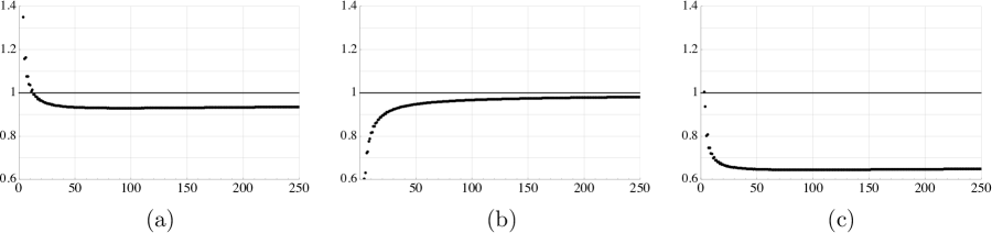
Figure 1: The three different estimates of $\log p_{n}/n!$, given by (a) Kotĕs̆ovec’s conjecture in equation (11), (b) the logarithm of the very accurate estimate from of equation (12), and (c) the accurate (but much slower to converge) estimate from equation (13).

In the illustration, the central item (b) shows that equation (12) gives a very accurate estimation. Furthermore, at first sight, the left item (a) shows that the estimation given by equation (11) is intuitively compatible with Kotĕs̆ovec’s conjecture 1.1, whereas the right item (c) shows that the estimation with equation (13) is slow to converge (but, perhaps surprisingly, will eventually converge to 1).

Computationally, obtaining the exact numerical values of the coefficients of $P(z)$ is very challenging for indices of order greater that $10^{3}$. Indeed, the entry A028342 in [36] has a table (attributed to Kotĕs̆ovec) that lists only the first 455 values of $a_{n}$. For these reasons, it is likely that Kotĕs̆ovec simply based his asymptotic estimate on a relatively small number of terms. It is also likely that he was not aware of the precise estimation given by equation (12).

We leverage the fact that the numeric value of $w_{n}$ can be obtained for very large values of $n$. It is easy to see that the logarithm of equation (12) is asymptotically equivalent to $w_{n}^{2}/2$, and the later is asymptotically equivalent to $(\log^{2}n)/2$; however, this asymptotic convergence is extremely slow. In Table 3, we illustrate values of $w_{n}^{2}/\log^{2}n$ for indices $n\leq 10^{3}$, and we emphasize that (in this range) they mainly exhibit a decreasing behavior, so it is easy to be misled about their asymptotic growth.

$n$	$2$	$3$	$4$	$6$	$8$	$10$	$20$	$50$	$10^{2}$	$10^{3}$
$w_{n}^{2}/\log^{2}n$	$2.7032$	$1.5433$	$1.2260$	$0.9957$	$0.9027$	$0.8522$	$0.7605$	$0.7100$	$0.6944$	$0.6899$

Table 3: List of values of $w_{n}^{2}/\log^{2}n$ for some $n\leq 10^{3}$.

If we divide the last entry in this table by $\log 2$, then we obtain $\frac{w_{1000}^{2}}{(\log 2)\log^{2}1000}=0.9954$, which may have led Kotĕs̆ovec to mistakenly include $\log{2}$ in his conjecture in equation (11), based on numerical evidence. However, in Table 4 we can look at the same values of $w_{n}^{2}/\log^{2}n$, for much larger indices $n\geq 10^{4}$. This allows us to see the slow asymptotic convergence that justifies that both estimates in Theorem 1.2 are accurate. Taken together with our proof (see Theorem 5.1), we confirm our numerical estimate of Theorem 1.2.

$n$	$10^{4}$	$10^{6}$	$10^{8}$	$10^{10}$	$10^{20}$	$10^{50}$	$10^{10^{2}}$	$10^{10^{3}}$	$10^{10^{4}}$	$10^{10^{5}}$
$w_{n}^{2}/\log^{2}n$	$0.7063$	$0.7437$	$0.7745$	$0.7987$	$0.8666$	$0.9295$	$0.9583$	$0.9937$	$0.9991$	$0.9998$

Table 4: List of values of $w_{n}^{2}/\log^{2}n$ for some $n\geq 10^{4}$.

The rest of the paper is organized as follows. In Section 2 we present a brief background on the study of partition functions. In Section 3 we describe, as labeled classes, the combinatorial structures enumerated by the (exponential) generating functions (1) and (2). In Section 4, we discuss the asymptotic analysis of these generating functions: First, we compute the Mellin transforms, which can be derived in a systematic way across the $(i,j,k)$ families. In contrast, the residue analysis needs to be customized for each triple parameter, though some generalities can be developed. The final asymptotic growth is obtained through saddle point method. With this methodology, we can resolve the conjectures about the asymptotic growth of the 6 sequences marked with (b) or (c) in Table 1. Additionally, we discover the asymptotic growth of the 9 sequences in OEIS that are marked with (d) in Table 1, and we provide the proofs.

2 Background

2.1 The partition problem

Ever since the work of Hardy and Ramanujan, there has been a continued and intensive development of the study of partition functions, there is a vast and diverse literature on the subject, the standard general reference is the book of Andrews [1] from 1984 and the references therein. The area has continued developing and we can only mention a brief list of some more recent works that are related, up to certain extends, to our context, like [25, 2, 8, 10, 3, 9, 24], works with more probabilistic points of view include [11, 19, 6, 13, 26], connexions with cellular automata can be found in [23], for other similar frameworks with $q$-series see [8], and so forth. There are several ways to generalizations, and in the literature several kinds of classes of functions are so called “weighted partitions”. For example, one kind arises by locating a sequence $(b_{n})_{n=1}^{\infty}$ of “weights” as coefficients, namely, products of the form

$$P(z)=\prod\limits_{n\geq 1}\frac{1}{1-b_{n}z^{n}}\qquad\textnormal{ and }\qquad Q(z)=\prod\limits_{n\geq 1}(1+b_{n}z^{n})$$ (14)

(see e.g. [39, 10, 9, 35, 12, 27, 28]). Another kind arises by locating a sequence $(a_{n})_{n\geq 1}$ of “weights” as exponents, namely, products of the form

$$P(z)=\prod\limits_{n\geq 1}\left(\frac{1}{1-z^{n}}\right)^{a_{n}}\qquad\textnormal{ and }\qquad Q(z)=\prod\limits_{n\geq 1}(1+z^{n})^{a_{n}}$$ (15)

(see e.g. [38, 40, 7, 32, 41, 19, 31, 20, 33]). A third kind could arise when putting the previous two kinds together, namely, products of the form

$$P(z)=\prod\limits_{n\geq 1}\left(\frac{1}{1-b_{n}z^{n}}\right)^{a_{n}}\qquad\textnormal{ and }\qquad Q(z)=\prod\limits_{n\geq 1}(1+b_{n}z^{n})^{a_{n}},$$ (16)

etc. In this paper, products of the second kind arise when $j=0$ (see Theorem 3.3), and also when the triple is $(i,j,k)=(0,1,0)$ (see Theorem 3.1), thus, in these cases there are certain sequences of weights as exponents. There have been several works that, under some general hypothesis, resolve the partition problem for families of sequences of weights as exponents (at least the first order asymptotic growth, and mostly focused, in fact, in the $\mathcal{P}$-form rather than the $\mathcal{Q}$-form). Probably the most famous result for sequences of weights as exponents is Meinardus’ Theorem [32] from 1954, which is also explained in depth in Theorem 6.2 of [1, Chapter 6, pp. 88]. Even before Meinardus, there are other works, such as Brigham [7] in 1950, that consider weighted partitions as a general framework for many types of partition problems. For example, he mentions well-known works of Wright [38, 40] from 1931 and 1934 as particular cases. Meinardus’ Theorem has been generalized, as in [18], see also [31], and for further works in this context see e.g. [4, 41, 42]. Nevertheless, the immense generalities make many cases to fall beyond the assumptions of well-known results like Meinardus’ Theorem and its generalizations, and some open conjectures on several partition problems that have been considered remain, as far as we know, unsolved, for instance see A028342  and A318413 in OEIS [36]. For example, in the case of the former, which is when $(i,j,k)=(0,1,0)$, what fails in Meinardus’ Theorem is the fact that a pole of $\zeta(s+1)$ is located at $0$. In the case of the later, or more generally, when the triple is $(i,0,k)$, then it is necessary to analyze the Dirichlet series $\sum_{n\geq 1}\frac{\psi(n)}{n^{s}}$, where $\psi(n)$ is defined in Theorem 3.1. The Meinardus style of argument is designed for the case of partitions of integers, that is, when the triple is $(i,j,k)=(0,0,1)$ (for this case, see again [1, Chapter 6]).

Furthermore, several other instances of open conjectures that fall within the scope of equations (1) and (2) are found in A168243, A107742, A280541, A318414, and we will present their resolutions. In virtue of Theorem 3.1, the general form of the “weighted partition function” that we are considering here has the form

$$\prod\limits_{n\geq 1}\exp\left(\frac{1}{n}\log\frac{1}{1-z^{n}}\right)^{a_{n}}$$ (17)

(the sequence $(a_{n})$ that yields equations (3) and (4) is $a_{n}=n$). Thus one of our goals here is to bring a source that resolves the conjectures regarding the partition problem in all these cases, in addition to verifying all claims.

2.2 Divisor functions

Recall that the well-known sum of divisors is the divisor function defined for every $n\geq 1$ by

$$\sigma_{x}(n):=\sum\limits_{d|n}d^{x}.$$ (18)

For example, $\sigma_{0}(n)$ is the number of divisors of $n$ and $\sigma(n):=\sigma_{1}(n)$ is the sigma function, i.e. the sum of the positive divosors of $n$. Also, for every $k\geq 1$, the $k$-fold number of divisors is the divisor function defined by

$$\tau_{k}(n):=\sum\limits_{d_{1}\cdots d_{k}=n}1.$$ (19)

In particular, $\tau_{1}(n)=1$ and $\tau(n):=\tau_{2}(n)=\sigma_{0}(n)$ (we let $\tau_{0}(n):=1$). Observe that

$$\tau_{k+1}(n):=\sum_{d|n}\tau_{k}(n/d).$$ (20)

Divisor functions are central in analytic number theory, in particular because of the well-known identity

$$\zeta(s)^{k}=\sum\limits_{n\geq 1}\frac{\tau_{k}(n)}{n^{s}},$$ (21)

i.e., $\zeta(s)^{k}$ is the Dirichlet series of $\big{(}\tau_{k}(n)\big{)}_{n\geq 1}$. For some recent developments see [34, 14, 5, 30].

3 Combinatorial specifications

In this section we present the general combinatorial specifications that yield the exponential generating functions given in equations (1) and (2). We will focus on the combinatorial class $\mathcal{P}$ and at the end of the section we will discuss the corresponding class $\mathcal{Q}$. When $j=0$ (i.e. there are no denominators), we get two alternative specifications that yield the same exponential generating functions, hence we obtain two isomorphic kinds of labeled combinatorial classes. We will describe several particular examples. We will be interested in coloring several objects with a countable set of different colors, as depicted in Figure 2. But first let us start with descriptions of certain basic classes in a way that will be useful throughout.

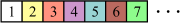
Figure 2: A countable list of different colors, labelled by $\{1,2,3,4,5,6,7,\ldots\}$.

3.1 Permutations, integer partitions, Young tableaux, and divisor diagrams

The combinatorial class $\mathcal{S}$ of all permutations can be specified as sets of labelled cycles, i.e.

$$\mathcal{S}(\mathcal{Z})=\hbox{{Set}}\big{(}\hbox{{Cyc}}(\mathcal{Z})\big{)},$$ (22)

which translates into the exponential generating function

$$\exp\left(\log\frac{1}{1-z}\right)=\frac{1}{1-z}.$$

For example, a permutation like

$$\left(\begin{tabular}[]{cccccccccccccccccccccccccccccccccc}1&2&3&4&5&6&7&8&9&10&11&12&13&14&15&16&17&18&19&20&21&22&23&24&25&26&27&28&29&30&31&32&33&34\\ 5&10&19&18&27&8&12&32&15&16&9&31&34&11&29&13&17&22&30&2&14&23&4&26&28&33&1&24&6&21&7&3&25&20\end{tabular}\right)$$ (25)

decomposes as a set of cycles coming from its decomposition as a product of cycles, namely,

$$(1\thinspace 5\thinspace 27)(2\thinspace 10\thinspace 16\thinspace 13\thinspace 34\thinspace 20)(3\thinspace 19\thinspace 30\thinspace 21\thinspace 14\thinspace 11\thinspace 9\thinspace 15\thinspace 29\thinspace 6\thinspace 8\thinspace 32)(4\thinspace 18\thinspace 22\thinspace 23)(7\thinspace 12\thinspace 31)(17)(24\thinspace 26\thinspace 33\thinspace 25\thinspace 28).$$ (26)

In general, we write cycles starting with the “leader”, and we can always “re-accommodate” the product of cycles monotonically in a unique way according to their lengths and, within cycles of equal length, according to the leader. For example,

$$(3\thinspace 19\thinspace 30\thinspace 21\thinspace 14\thinspace 11\thinspace 9\thinspace 15\thinspace 29\thinspace 6\thinspace 8\thinspace 32)(2\thinspace 10\thinspace 16\thinspace 13\thinspace 34\thinspace 20)(24\thinspace 26\thinspace 33\thinspace 25\thinspace 28)(4\thinspace 18\thinspace 22\thinspace 23)(1\thinspace 5\thinspace 27)(7\thinspace 12\thinspace 31)(17).$$ (27)

Any permutation is associated to an integer partition of its size, namely the lengths of its cycles, e.g. for the permutation above we have the partition $34=12+6+5+4+3+3+1$. It is customary to represent integer partitions as Young diagrams, i.e. as monotone arrangements of horizontal blocks formed by consecutive boxes with lengths according to the summands in the partition. See item (a) in Figure 3 for the example above (observe that, for reference, the associated partition is written to the left of the Young diagram).

Figure 3: Young Tableaux: (a) A Young diagram. (b) A Young tableau. (c) A Young tableau obtained from (b) by cyclically shifting some rows. (d) A Young tableau obtained from (b) by switching rows of the same size.

A Young tableau on a Young diagram of size $n$ is a well-labelling of the boxes of the Young diagram with the set $\{1,\ldots,n\}$ (then, all the $n$ symbols are required to be used exactly once). For example, (b) in Figure 3 is the unique representation (described before) of the partition given as in equation (27). In fact, every Young tableau has an associated permutation which has the labelled rows as its decomposition in cycles. Thus, different labelling of Young diagrams can yield Young tableaux that have the same associated permutation, for example in Figure 3, items (b) and (c) differ only because some rows were shifted cyclically, that is, the permutation remains invariant under the action $\alpha$ by cyclic shifts, that is, $\alpha(a_{1},\dots,a_{n})=(a_{2},\ldots a_{n},a_{1})$ for every $(a_{1},\ldots,a_{n})\in\mathcal{A}^{n}$. A class of Young tableaux is modular if its elements are regarded as equivalence classes of the equivalence relation defined by the $\alpha$-orbits. Similarly, in Figure 3, items (b) and (d) differ only by a permutation of the two rows of length three, the other generic instance that make two different Young tableaux induce the same permutation. Thus there is also an action $\sigma$ that for every $n\geq 1$ acts by permutations on the set of $n$-blocks, and the original permutation is also invariant under this $\sigma$-action. A class of Young tableaux is symmetric if its elements are regarded as equivalence classes of the orbital equivalence relation induced by the $\sigma$-action. Thus for example, the class $\mathcal{S}$ of all permutations is represented by the class of modular and symmetric Young tableaux.

The divisor diagram associated to a Young diagram is again an arrangement of blocks of boxes arranged as rows beside the Young diagram in a way that blocks of length $n$ in the Young diagram correspond to blocks of length $\tau(n)$ in the divisor diagram (it is like the “image” of the Young diagram under the number of divisor function $\tau(n)$, thus, in general, the arrangement in the divisor diagram is not monotone). See Figure 4.

Figure 4: A Young diagram together with its divisor diagram.

Henceforth, the divisors of a positive integer $n$ will be written as $1=p_{1}<\ldots<p_{\tau(n)}=n$.

Remark 28.

Observe that for any box in the $l$th column of the divisor diagram, if it belongs to a block of size $n$, then $\tau(p_{l})=l$.

3.2 General combinatorial specifications for $\mathcal{P}$

Let us formally give the two main global combinatorial specifications.

Theorem 3.1.

For every admissible triple $(i,j,k)$, define for every positive integer $n$ the arithmetic function

$$\chi(n):=\begin{cases}n^{2}\cdot\tau_{i}(n)\quad&\textnormal{for }(i\geq 1,0,0)\vskip 3.0pt plus 1.0pt minus 1.0pt\\ n\sum\limits_{\ell=1}^{\tau(n)}p_{\ell}\cdot\tau_{i}(p_{\ell})\cdot\tau_{k}(n/p_{\ell})\quad&\textnormal{for }(i\geq 1,0,k\geq 1)\vskip 3.0pt plus 1.0pt minus 1.0pt\\ \sum\limits_{\ell=1}^{\tau(n)}p_{\ell}^{2}\cdot\tau_{i}(p_{\ell})\cdot\tau_{j}(n/p_{\ell})\quad&\textnormal{for }(i\geq 1,j\geq 1,0)\vskip 3.0pt plus 1.0pt minus 1.0pt\\ \sum\limits_{\ell=1}^{\tau(n)}\sum\limits_{m=1}^{\tau(n/p_{\ell})}p_{\ell}^{2}q_{m}\cdot\tau_{i}(p_{\ell})\cdot\tau_{k}(q_{m})\cdot\tau_{j}\big{(}n/(p_{\ell}q_{m})\big{)}\quad&\textnormal{for }(i\geq 1,j\geq 1,k\geq 1)\\ n\cdot\tau_{k}(n)\quad&\textnormal{for }(0,0,k\geq 1)\vskip 3.0pt plus 1.0pt minus 1.0pt\\ \sum\limits_{\ell=1}^{\tau(n)}p_{\ell}\cdot\tau_{k}(p_{\ell})\cdot\tau_{j}(n/p_{\ell})\quad&\textnormal{for }(0,j\geq 1,k\geq 1)\vskip 3.0pt plus 1.0pt minus 1.0pt\\ \tau_{j}(n)\quad&\textnormal{for }(0,j\geq 1,0)\vskip 3.0pt plus 1.0pt minus 1.0pt\\ \end{cases}$$ (29)

where $q_{m}|\frac{n}{p_{\ell}}$ for $m=1,\ldots,\tau(n/p_{\ell})$ are the divisors of $n/p_{\ell}$. Then $P(z)$ is the cyclic Euler transform of $\chi(n)$, that is,

$$P(z)=\prod_{n\geq 1}\exp\left(\sum\limits_{\ell=1}^{\infty}\frac{z^{n\ell}}{n\ell}\right)^{\chi(n)}.$$ (30)

Proof.

We have

$$P(z) =\prod\left(\frac{1}{1-z^{n_{1}\cdots n_{i}d_{1}\cdots d_{j}e_{1}\cdots e_{k}}}\right)^{n_{1}\cdots n_{i}/d_{1}\cdots d_{j}}$$ (31)

$$=\prod\exp\left(\log\left(\left(\frac{1}{1-z^{n_{1}\cdots n_{i}d_{1}\cdots d_{j}e_{1}\cdots e_{k}}}\right)^{n_{1}\cdots n_{i}/d_{1}\cdots d_{j}}\right)\right)$$ (32)

$$=\prod\exp\left(\frac{1}{d_{1}\cdots d_{j}}\log\left(\frac{1}{1-z^{n_{1}\cdots n_{i}d_{1}\cdots d_{j}e_{1}\cdots e_{k}}}\right)\right)^{n_{1}\cdots n_{i}}$$ (33)

$$=\prod\exp\left(\frac{1}{d_{1}\cdots d_{j}}\sum\limits_{\ell=1}^{\infty}\frac{z^{n_{1}\cdots n_{i}d_{1}\cdots d_{j}e_{1}\cdots e_{k}\ell}}{\ell}\right)^{n_{1}\cdots n_{i}}$$ (34)

$$=\prod\exp\left(n_{1}\cdots n_{i}e_{1}\cdots e_{k}\sum\limits_{\ell=1}^{\infty}\frac{z^{n_{1}\cdots n_{i}d_{1}\cdots d_{j}e_{1}\cdots e_{k}\ell}}{n_{1}\cdots n_{i}d_{1}\cdots d_{j}e_{1}\cdots e_{k}\ell}\right)^{n_{1}\cdots n_{i}}$$ (35)

$$=\prod\exp\left(\sum\limits_{\ell=1}^{\infty}\frac{z^{n_{1}\cdots n_{i}d_{1}\cdots d_{j}e_{1}\cdots e_{k}\ell}}{n_{1}\cdots n_{i}d_{1}\cdots d_{j}e_{1}\cdots e_{k}\ell}\right)^{(n_{1}\cdots n_{i})^{2}\cdot e_{1}\cdots e_{k}}$$ (36)

and hence the result follows. ∎

Corollary 3.2.

The exponential generating function in equation (1) comes from the specification

$$\mathcal{P}(\mathcal{Z})=\prod\limits_{n=1}^{\infty}\hbox{{Seq}}_{\chi(n)}\left(\hbox{{Set}}\left(\bigcup_{\ell=1}^{\infty}\hbox{{Cyc}}_{n\ell}(\mathcal{Z})\right)\right).$$ (37)

Only when $j>0$ we are forced to consider cycles. Thus the case $j=0$ deserves its own attention. In fact we will see now, in the result that follows, that in this case $\mathcal{P}$ admits a specification that translates into a representation of $P(z)$ with the form given in Meinardus’ Theorem (thus the later could be applied if all its hypothesis are satisfied); the proof of this result and the next two that follow are now straightforward.

Theorem 3.3.

For every positive integer $n$, let

$$\psi(n):=\begin{cases}n\cdot\tau_{i}(n)\quad&\textnormal{for }(i\geq 1,0,0)\vskip 3.0pt plus 1.0pt minus 1.0pt\\ \tau_{k}(n)\quad&\textnormal{for }(0,0,k\geq 1)\vskip 3.0pt plus 1.0pt minus 1.0pt\\ \sum\limits_{\ell=1}^{\tau(n)}p_{\ell}\cdot\tau_{i}(p_{\ell})\cdot\tau_{k}(n/p_{\ell})\quad&\textnormal{for }(i\geq 1,0,k\geq 1).\end{cases}$$ (38)

If $j=0$, then $P(z)$ is the Euler transform of $\psi(n)$, that is,

$$P(z) =\prod\left(\frac{1}{1-z^{n_{1}\cdots n_{i}e_{1}\cdots e_{k}}}\right)^{n_{1}\cdots n_{i}}=\prod_{n\geq 1}\left(\frac{1}{1-z^{n}}\right)^{\psi(n)}.$$ (39)

Corollary 3.4.

The exponential generating function in equation (2) comes from the specification

$$\mathcal{P}(\mathcal{Z})=\prod\limits_{n=1}^{\infty}\hbox{{Seq}}_{\psi(n)}\big{(}\hbox{{Seq}}(\mathcal{Z}^{n})\big{)}.$$ (40)

Proposition 3.5.

Given an admissible triple $(i,0,k)$, the combinatorial classes defined by equations (37) and (40) are isomorphic.

3.3 Examples

So, let us now see several examples to better understand the labeled structures defined by equations (37) and (40). Let us start with the cases that force an exponential context, i.e. when $j\geq 1$. Actually, in virtue of Theorem 3.1, analyzing the first few cases suffices to understand the whole class described in equation (37).

3.3.1 Colored permutations by number of divisors: $(0,1,0)$

Consider the case $(i,j,k)=(0,1,0)$. This is the case of Theorem 1.2. In this case, the specification in equation (37) becomes

$$\mathcal{P}(\mathcal{Z})=\prod_{n=1}^{\infty}\hbox{{Set}}\Big{(}\bigcup_{\ell=1}^{\infty}\hbox{{Cyc}}_{n\ell}(\mathcal{Z})\Big{)}$$ (41)

(compare with (22)). It represents the class of permutations, but now they carry a label on each cycle which is a divisor of that cycle’s length. For instance,

$$\overbrace{(3\thinspace 19\thinspace 30\thinspace 21\thinspace 14\thinspace 11\thinspace 9\thinspace 15\thinspace 29\thinspace 6\thinspace 8\thinspace 32)}^{3|12}\overbrace{(2\thinspace 10\thinspace 16\thinspace 13\thinspace 34\thinspace 20)}^{2|6}\overbrace{(24\thinspace 26\thinspace 33\thinspace 25\thinspace 28)}^{1|5}\overbrace{(4\thinspace 18\thinspace 22\thinspace 23)}^{4|4}\overbrace{(1\thinspace 5\thinspace 27)}^{3|3}\overbrace{(7\thinspace 12\thinspace 31)}^{1|3}\overbrace{(17)}^{1|1}.$$ (42)

Any such set of labels showing an example divisor of each cycle length is suitable. For instance, another element of size 34 is

$$\overbrace{(3\thinspace 19\thinspace 30\thinspace 21\thinspace 14\thinspace 11\thinspace 9\thinspace 15\thinspace 29\thinspace 6\thinspace 8\thinspace 32)}^{12|12}\overbrace{(2\thinspace 10\thinspace 16\thinspace 13\thinspace 34\thinspace 20)}^{3|6}\overbrace{(24\thinspace 26\thinspace 33\thinspace 25\thinspace 28)}^{5|5}\overbrace{(4\thinspace 18\thinspace 22\thinspace 23)}^{2|4}\overbrace{(1\thinspace 5\thinspace 27)}^{1|3}\overbrace{(7\thinspace 12\thinspace 31)}^{1|3}\overbrace{(17)}^{1|1}$$ (43)

We emphasize that any label of the form $p|l$ above a cycle of length $l$ is valid. In other words, an element of $\mathcal{P}$ is completely determined by the structure of the cycles in that permutation, and the choice of one divisor (indeed, any divisor $p$) of each cycle length. The choice of divisors is equivalent to coloring each row of length $n$ of the corresponding Young diagram with $\tau(n)$ colors, e.g. see Figure 5. So in this case the structure is the class of colored permutations with divisor function $\tau(n)$, that is, colored permutations by number of divisors. Its first elements are shown in Figure 6.

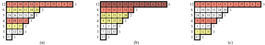
Figure 5: Colored permutations by number of divisors (the numbering on the right of each row corresponds to the color number). (a) Coloring according to equation (42) (b) Coloring according to equation (43). (c) Another legal coloring.

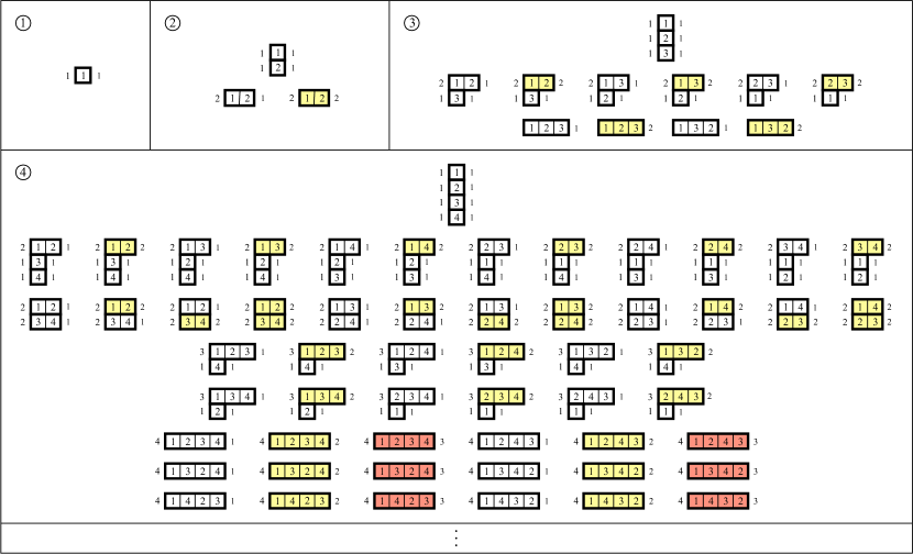
Figure 6: The first elements of colored permutations by number of divisors.

3.3.2 Colored permutations by number of divisors with rooted colorings of divisor diagrams by number of divisors: $(0,2,0)$

Consider the case $(i,j,k)=(0,2,0)$. In this case we obtain the specification

$$\mathcal{P}(\mathcal{Z})=\prod_{n=1}^{\infty}\hbox{{Seq}}_{\tau(n)}\left(\hbox{{Set}}\left(\bigcup\limits_{\ell=1}^{\infty}\hbox{{Cyc}}_{n\ell}(\mathcal{Z})\right)\right).$$ (44)

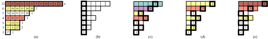
Figure 7: A colored permutation by number of divisors together with four instances of rooted colorings of its divisor diagram by number of divisors. (a) A colored partition in a Young diagram. (b), (c), (d) Three different rooted colorings of the divisor diagram associated to the Young diagram in (a).

Keeping in mind the case $(0,1,0)$ in Section 3.3.1, we see that again we get colored permutations by number of divisors, but now, in addition, each block in the Young diagram carries an additional label, namely, for each block of length $n$, if we list the divisors of $n$ as $1=p_{1}<\ldots<p_{\tau(n)}=n$ and then pick one divisor $p_{l}$, then the label is a color chosen from a set of colors of size of $\tau(p_{l})=l$ (see Remark 28), and this can be pictured as colorings of rooted divisor diagrams by size. So in this case, if the $l$th box of a block is the root, then the size of the set of colors is $l$. See Figure 7 for instance, it shows a colored permutation and four instances of rooted colorings of its divisor diagram by number of divisors. If the first box is chosen as the root for all blocks, then there is only one coloring, the monochromatic, and this is the case shown in item (b) in this figure. Items (c), (d) and (e) show other possible rooted colorings of the divisor diagram.

3.3.3 Colored permutations by number of divisors with rooted colorings of divisor diagram with divisor function $\chi(n)$: $(i,j,k)$

With the two previous examples on mind, now we can understand the general case in equation (37) because it only differs from the specification in equation (44) by the divisor function $\chi(n)$ instead of the divisor function $\tau(n)$ in the sequence operator. Thus, the structure is essentially the same, that is, the class consists again of colored permutations by number of divisors, and the difference is that the coloring of the rooted divisor diagram is now determined by the divisor function $\chi(n)$. To be precise, if the $l$th box in a block of the divisor diagram that is associated to an $n$-block in the Young diagram has been chosen as the root, and if the divisors of $n$ are written as $1=p_{1}<\ldots<p_{\tau(n)}=n$, then the block of the divisor diagram is colored with a set of colors of size $\chi(p_{l})$. Note that in the general case, if two distinct boxes in the $l$th column of the divisor diagram are chosen as roots of their corresponding blocks, then the blocks may be colored with sets of colors of distinct cardinalities.

Now it is turn to analyze the specification given in equation (40).

3.3.4 Ordered colorings of Young tableaux by size: $(1,0,0)$

Now consider the triple $(i,j,k)=(1,0,0)$. In this case, $P(z)$ is known to be the ordinary generating function of the plane partitions, studied by Wright (see [38]). In a labelled universe, the class consists of well colorings of plane partitions and is combinatorially isomorphic to the (isomorphic) classes that result from the specifications given in equations (37) and (40). The later becomes

$$\mathcal{P}(\mathcal{Z})=\prod_{n=1}^{\infty}\hbox{{Seq}}_{n}\left({\hbox{{Seq}}(\mathcal{Z}^{n})}\right)$$ (45)

and it translates into

$$P(z)=\prod_{n=1}^{\infty}\frac{1}{(1-z^{n})^{n}}.$$ (46)

In this case, the labelled class $\mathcal{P}$, as specified in equation (45), consists of colorings of Young tableaux by size, i.e. the blocks of size $n$ are colored with $n$ distinct colors. See Figure 8 for examples. Note the difference with the colored permutations by number of divisors from Section 3.3.1 in that here the Young tableaux are colored by size and they are not modular nor symmetric. Furthermore, in this case we also have $\chi(n)=n^{2}\tau_{1}(n)=n^{2}$, thus, according to Proposition 3.5, the class of colored Young tableaux by size is isomorphic to the class of colored permutations by number of divisors with rooted colorings of divisor diagrams by size squared.

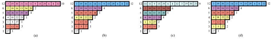
Figure 8: Colored Young tableaux by size. Each row of length $n$ is colored with a set of colors of size $n$. (a) A colored Young tableau by size function. (b) Another colored Young tableau, it differs from (a) not only from the coloring, but also the labelling of the rows of size three have been permuted, i.e. the Young tableaux are not symmetric. (c) Another colored Young tableau, it differs from (a) not only from the coloring, but also a row has been cyclically shifted, i.e. the Young tableaux are not modular. (d) Another coloring of another Young tableau.

3.3.5 Colored Young tableaux by divisor function $\psi(n)$: $(i,0,k)$

The specification in equation (40) for the general case of triples $(i,0,k)$ differs from the previos example in that $\psi(n)$ now replaces the size function $n$. In other words, we get again colored Young tableaux like in Section 3.3.4, the only difference is that now the size of the set of colors used to color the set of $n$-blocks is the divisor function $\psi(n)$ (indeed, when $i=1$ and $k=0$, $\psi(n)=n$, i.e. $\psi(n)$ is the size). Again we recall that this class is isomorphic to the class of colored permutations by number of divisors with with rooted colorings of divisor diagrams with divisor function $\chi(n)$.

3.4 The class $\mathcal{Q}$

With the two global combinatorial perspectives for $\mathcal{P}$ given by the specifications in equation (37) and (40), we can give a general description of the corresponding class $\mathcal{Q}$ with markers and bivariate (exponential) generating functions as follows. First consider a weighted version of equation (37), namely, the specification

$$\widehat{\mathcal{P}}(\mathcal{Z},\mathcal{V})=\prod\limits_{n=1}^{\infty}\hbox{{Seq}}_{\chi(n)}\left(\hbox{{Set}}\left(\bigcup_{\ell=1}^{\infty}\mathcal{V}^{\ell+1}\hbox{{Cyc}}_{n\ell}(\mathcal{Z})\right)\right).$$ (47)

The corresponding bivariate (exponential) generating function $\widehat{P}(z,v)$ is therefore

$$\widehat{P}(z,v)=\prod_{n=1}^{\infty}\exp\left(\sum_{\ell=1}^{\infty}v^{\ell+1}\frac{z^{n\ell}}{n\ell}\right)^{\chi(n)}.$$ (48)

In the case $v=1$, we have already seen (in equation (30)) that $\widehat{P}(z,1)=P(z)$. Now set the weight $v=-1$ and follow the proof of Theorem 3.1 backwards to get

$$\widehat{P}(z,-1) =\prod_{n=1}^{\infty}\exp\left(\sum_{\ell=1}^{\infty}(-1)^{\ell+1}\frac{z^{n\ell}}{n\ell}\right)^{\chi(n)}$$ (49)

$$=\prod\exp\left(-\sum\limits_{\ell=1}^{\infty}\frac{(-z^{n_{1}\cdots n_{i}d_{1}\cdots d_{j}e_{1}\cdots e_{k}})^{\ell}}{n_{1}\cdots n_{i}d_{1}\cdots d_{j}e_{1}\cdots e_{k}\ell}\right)^{(n_{1}\cdots n_{i})^{2}\cdot e_{1}\cdots e_{k}}$$ (50)

$$=\prod\exp\left(-\sum\limits_{\ell=1}^{\infty}\frac{(-z^{n_{1}\cdots n_{i}d_{1}\cdots d_{j}e_{1}\cdots e_{k}})^{\ell}}{\ell}\right)^{n_{1}\cdots n_{i}/d_{1}\cdots d_{j}}$$ (51)

$$=\prod\exp\left(-\log\frac{1}{1+z^{n_{1}\cdots n_{i}d_{1}\cdots d_{j}e_{1}\cdots e_{k}}}\right)^{n_{1}\cdots n_{i}/d_{1}\cdots d_{j}}$$ (52)

$$=Q(z).$$ (53)

More generally, however, if we fix the value of the weights $v$, we get

$$P_{n}^{(v)}=[z^{n}]\widehat{P}(z,v)=[z^{n}]\prod_{n=1}^{\infty}\exp\left(\sum_{\ell=1}^{\infty}v^{\ell+1}\frac{z^{n\ell}}{n\ell}\right)^{\chi(n)}=[z^{n}]\prod_{\delta=1}^{\infty}\exp\Bigg{(}\sum_{\ell\geq 1\atop{\rm with\!\ }\delta|\ell}^{\infty}v^{\frac{\ell}{\delta}+1}\frac{z^{\ell}}{\ell}\Bigg{)}^{\chi(\delta)}.$$ (54)

As seen above, the coefficients $Q_{n}=[z^{n}]Q(z)$ can be calculated as a sum of weighted terms (with weights $+1$ and $-1$) of coefficients from $P(z)$. Since $v=1$ yields $\widehat{P}(z,1)=P(z)$ and $v=-1$ yields $\widehat{P}(z,-1)=Q(z)$, it would be interesting to explore other exponential generating functions of the form $\widehat{P}(z,v)$ for other roots of unity $v=e^{i\theta}$ on the unit circle. We leave such explorations as open problems.

4 Asymptotic analysis

The asyptotic analysis is carried out in a similar way as in [17]. Let us start with the substitution $z\triangleq e^{-t}$. Let $L_{P}(t)=\log\big{(}P(e^{-t})\big{)}$ and $L_{Q}(t)=\log\big{(}Q(e^{-t})\big{)}$. Also, let $L(t)$ denote either $L_{P}(t)$ or $L_{Q}(t)$.

4.1 Mellin transforms

As a general reference to Mellin transforms, see [37, Ch. 9].

Proposition 4.1 (Mellin transform for $\mathcal{P}$ and $\mathcal{Q}$).

Let $L_{P}^{*}(s):={\mathcal{M}}[L_{P}(t);s]$ and $L_{Q}^{*}(s):={\mathcal{M}}[L_{Q}(t);s]$ be the Mellin transforms of $L_{P}(t)$ and $L_{Q}(t)$, respectively. These Mellin transforms have the succinct forms

$$L_{P}^{*}(s)=\zeta(s-1)^{i}\zeta(s+1)^{j+1}\zeta(s)^{k}\Gamma(s)$$ (55)

and

$$L_{Q}^{*}(s)=(1-2^{-s})\zeta(s-1)^{i}\zeta(s+1)^{j+1}\zeta(s)^{k}\Gamma(s).$$ (56)

Proof.

We have $L_{P}(t)=\log\big{(}P(e^{-t})\big{)}=\log\prod(1-e^{-tn_{1}\cdots n_{i}d_{1}\cdots d_{j}e_{1}\cdots e_{k}})^{-n_{1}\cdots n_{i}/d_{1}\cdots d_{j}}$, by the definition of $L_{P}$ and $P$. The log of the product equals the sum of the logs, and it follows that $L_{P}(t)=\sum\frac{n_{1}\cdots n_{i}}{d_{1}\cdots d_{j}}\log(1/(1-e^{-tn_{1}\cdots n_{i}d_{1}\cdots d_{j}e_{1}\cdots e_{k}}))$. Then we can expand the log as a series, and exchange the order of the summations, to obtain $L_{P}(t)=\sum_{j=1}^{\infty}\frac{1}{j}\sum\frac{n_{1}\cdots n_{i}}{d_{1}\cdots d_{j}}e^{-tn_{1}\cdots n_{i}d_{1}\cdots d_{j}e_{1}\cdots e_{k}j}$. By linearity of the Mellin transform, we have $L_{P}^{*}(s)=\sum_{j=1}^{\infty}\frac{1}{j}\sum\frac{n_{1}\cdots n_{i}}{d_{1}\cdots d_{j}}{\mathcal{M}}\left[e^{-tn_{1}\cdots n_{i}d_{1}\cdots d_{j}e_{1}\cdots e_{k}j};s\right]$. Using scaling for the Mellin transform [37, equation (9.5)], we have ${\mathcal{M}}\left[e^{-tn_{1}\cdots n_{i}d_{1}\cdots d_{j}e_{1}\cdots e_{k}j};s\right]=(n_{1}\cdots n_{i}d_{1}\cdots d_{j}e_{1}\cdots e_{k}j)^{-s}{\mathcal{M}}\left[e^{-t};s\right]$. It is well known that ${\mathcal{M}}\left[e^{-t};s\right]=\Gamma(s)$. So it follows that $L_{P}^{*}(s)=\sum_{j=1}^{\infty}\frac{1}{j}\sum\frac{n_{1}\cdots n_{i}}{d_{1}\cdots d_{j}}\cdot(n_{1}\cdots n_{i}d_{1}\cdots d_{j}e_{1}\cdots e_{k}j)^{-s}\Gamma(s)$, which simplifies to

$$L_{P}^{*}(s)=\zeta(s-1)^{i}\zeta(s+1)^{j+1}\zeta(s)^{k}\Gamma(s).$$

The analysis for $L_{Q}(t)$ is similar. We have $L_{Q}(t)=\log\prod(1+e^{-tn_{1}\cdots n_{i}d_{1}\cdots d_{j}e_{1}\cdots e_{k}})^{n_{1}\cdots n_{i}/d_{1}\cdots d_{j}}$. Then we expand as before, and we get $L_{Q}(t)=\sum_{j=1}^{\infty}\frac{(-1)^{j+1}}{j}\sum\frac{n_{1}\cdots n_{i}}{d_{1}\cdots d_{j}}e^{-tn_{1}\cdots n_{i}d_{1}\cdots d_{j}e_{1}\cdots e_{k}j}$. Again using linearity and scaling, it follows that $L_{Q}^{*}(s)=\sum_{j=1}^{\infty}\frac{(-1)^{j+1}}{j}\sum\frac{n_{1}\cdots n_{i}}{d_{1}\cdots d_{j}}\cdot(n_{1}\cdots n_{i}d_{1}\cdots d_{j}e_{1}\cdots e_{k}j)^{-s}\Gamma(s)$, which simplifies to $L_{Q}^{*}(s)=\eta(s+1)\zeta(s-1)^{i}\zeta(s+1)^{j}\zeta(s)^{k}\Gamma(s)$, where $\eta(s)=\sum_{n=1}^{\infty}\frac{(-1)^{n+1}}{n^{s}}$ is the Dirichlet eta function. For symmetry with the equation for $L_{P}^{*}(s)$, we transform this to:

$$L_{Q}^{*}(s)=(1-2^{-s})\zeta(s-1)^{i}\zeta(s+1)^{j+1}\zeta(s)^{k}\Gamma(s).$$

∎

Henceforth, let $L^{*}(s)$ denote either $L^{*}_{P}(s)$ or $L_{Q}^{*}(s)$.

4.2 Singularity analysis

We make a handful of singularity analysis observations.

Proposition 4.2.

The following hold:

1. If $i\geq 1$, then $L^{*}(s)$ has a singularity at $s=2$ generated by $\zeta(s-1)^{i}$. It is a pole of order $i\geq 1$, because the remaining terms in equations (55) and (56) are nonzero at $s=2$.

2. If $k\geq 1$, then $L^{*}(s)$ has a singularity at $s=1$ generated by $\zeta(s)^{k}$. It is a pole of order $k\geq 1$ because the remaining terms terms in equations (55) and (56) are nonzero at $s=1$.

3. Both $L_{P}^{*}(s)$ and $L_{Q}^{*}(s)$ have a singularity at $s=0$ generated by $\zeta(s+1)^{j+1}\Gamma(s)$. The singularity of $L_{P}^{*}(s)$ at $s=0$ is a pole of order $j+2\geq 2$ because the remaining terms in (55) are nonzero at $s=0$. In contrast, since $1-2^{-s}$ has a simple zero at $s=0$, then the singularity of $L_{Q}^{*}(s)$ at $s=0$ is a pole of order $j+1\geq 1$ because the remaining terms in (56) are nonzero at $s=0$.

4. If $i=0$, then $L^{*}(s)$ has a singularity at $s=-1$ generated by $\Gamma(s)$. It is a simple pole because the remaining terms in (55) and (56) are nonzero at $s=-1$. On the other hand, if $i\geq 1$, then the simple pole at $s=-1$ generated by $\Gamma(s)$ is cancelled by the zero of order $i\geq 1$ in $\zeta(s-1)^{i}$.

5. If $k=0$, then $L^{*}(s)$ has a singularity at $s=-2n$ for each $n\geq 1$, generated by $\Gamma(s)$. It is a simple pole because the remaining terms in (55) and (56) are nonzero at $s=-2n$. On the other hand, if $k\geq 1$, then the singularity at $s=-2n$ is cancelled by the zero of order $k\geq 1$ in $\zeta(s)^{k}$.

6. For each $n\geq 1$, the simple pole at $s=-(2n+1)$ generated by $\Gamma(s)$ is cancelled by the zero of order $j+1\geq 1$ in $\zeta(s+1)^{j+1}$.

4.3 Residue analysis

Proposition 4.3.

For all $i\geq 1$ and $j\geq 0$ and $k\geq 0$, there is a computable polynomial $a(t)=a_{0}+\ldots+a_{i-1}t^{i-1}$ such that

$${\operatorname{Res}}\big{(}L^{*}(s)t^{-s}\big{)}_{s=2}=\frac{a(\log t)}{t^{2}}.$$

For $L_{P}^{*}(s)$ and $L_{Q}^{*}(s)$ respectively, the values of $a_{i-1}$ are

$$\frac{(-1)^{i-1}\zeta(3)^{j+1}\pi^{2k}}{6^{k}(i-1)!}\qquad\hbox{and}\qquad\frac{(3)(-1)^{i-1}\zeta(3)^{j+1}\pi^{2k}}{(4)(6^{k})(i-1)!}.$$ (57)

We use $a_{i-1}$ very often in the following discussion, so we define $A:=a_{i-1}$ (so that the dependence on the values of $i$ and $j$ and $k$ is implicit; we also treat the relationship to $P$ or $Q$ as implicit).

Proof.

We first note that ${\operatorname{Res}}\big{(}\zeta(s+1)^{i}t^{-s}\big{)}_{s=0}$ is a polynomial in $\log{t}$ of degree $i-1$, with leading coefficient $\frac{(-1)^{i-1}}{(i-1)!}$. So we have

$${\operatorname{Res}}\big{(}\zeta(s+1)^{i}t^{-s}\big{)}_{s=0}=\frac{(-1)^{i-1}}{(i-1)!}(\log{t})^{i-1}+o((\log{t})^{i-1}).$$

At $s=0$, we note that $\zeta(s+3)^{j+1}$, $\zeta(s+2)^{k}$, and $\Gamma(s+2)$ are all smooth, and also that $\zeta(2)=\pi^{2}\!/6$ and $\Gamma(2)=1$. It follows that

$${\operatorname{Res}}\big{(}\zeta(s+1)^{i}\zeta(s+3)^{j+1}\zeta(s+2)^{k}\Gamma(s+2)t^{-s}\big{)}_{s=0}=\frac{(-1)^{i-1}\zeta(3)^{j+1}\pi^{2k}}{6^{k}(i-1)!}(\log{t})^{i-1}+o((\log{t})^{i-1}).$$

Shifting $s$ by 2, the LHS becomes ${\operatorname{Res}}\big{(}\zeta(s-1)^{i}\zeta(s+1)^{j+1}\zeta(s)^{k}\Gamma(s)t^{-(s-2)}\big{)}_{s=2}=t^{2}{\operatorname{Res}}\big{(}L_{P}^{*}(s)t^{-s}\big{)}_{s=2}$ so we obtain

$${\operatorname{Res}}\big{(}L_{P}^{*}(s)t^{-s}\big{)}_{s=2}=\frac{1}{t^{2}}\bigg{(}\frac{(-1)^{i-1}\zeta(3)^{j+1}\pi^{2k}}{6^{k}(i-1)!}(\log{t})^{i-1}+o((\log{t})^{i-1})\bigg{)}.$$

At $s=2$, we also note that $1-2^{-s}=3/4$, so we obtain

$${\operatorname{Res}}\big{(}L_{Q}^{*}(s)t^{-s}\big{)}_{s=2}=\frac{1}{t^{2}}\bigg{(}\frac{(3)(-1)^{i-1}\zeta(3)^{j+1}\pi^{2k}}{(4)(6^{k})(i-1)!}(\log{t})^{i-1}+o((\log{t})^{i-1})\bigg{)}.$$

∎

Proposition 4.4.

For all $i\geq 0$ and $j\geq 0$ and $k\geq 1$, there is a computable polynomial $b(t)=b_{0}+\ldots+b_{k-1}t^{k-1}$ such that

$${\operatorname{Res}}\big{(}L^{*}(s)t^{-s}\big{)}_{s=1}=\frac{b(\log t)}{t}.$$

For $L_{P}^{*}(s)$ and $L_{Q}^{*}(s)$ respectively, the values of $b_{k-1}$ are

$$\frac{(-1)^{i+k-1}\pi^{2(j+1)}}{6^{j+1}2^{i}(k-1)!}\qquad\hbox{and}\qquad\frac{(-1)^{i+k-1}\pi^{2(j+1)}}{6^{j+1}2^{i+1}(k-1)!}.$$ (58)

We define $B:=b_{k-1}$ (the dependence on $i,j,k$ and on $P$ or $Q$ is implicit).

Proof.

Using exactly the same observation as from the previous proposition, we first note that ${\operatorname{Res}}\big{(}\zeta(s+1)^{k}t^{-s}\big{)}_{s=0}$ is a polynomial in $\log{t}$ of degree $k-1$, with leading coefficient $\frac{(-1)^{k-1}}{(k-1)!}$. So we have

$${\operatorname{Res}}\big{(}\zeta(s+1)^{k}t^{-s}\big{)}_{s=0}=\frac{(-1)^{k-1}}{(k-1)!}(\log{t})^{k-1}+o((\log{t})^{k-1}).$$

At $s=0$, we note that $\zeta(s)^{i}$, $\zeta(s+2)^{j+1}$, and $\Gamma(s+1)$ are all smooth, and also that $\zeta(0)=-1/2$ and $\zeta(2)=\pi^{2}\!/6$ and $\Gamma(1)=1$. It follows that

$${\operatorname{Res}}\big{(}\zeta(s)^{i}\zeta(s+2)^{j+1}\zeta(s+1)^{k}\Gamma(s+1)t^{-s}\big{)}_{s=0}=\frac{(-1)^{i+k-1}\pi^{2(j+1)}}{6^{j+1}2^{i}(k-1)!}(\log{t})^{k-1}+o((\log{t})^{k-1}).$$

Shifting $s$ by 1, the LHS becomes ${\operatorname{Res}}\big{(}\zeta(s-1)^{i}\zeta(s+1)^{j+1}\zeta(s)^{k}\Gamma(s)t^{-(s-1)}\big{)}_{s=1}=t{\operatorname{Res}}\big{(}L_{P}^{*}(s)t^{-s}\big{)}_{s=1}$ so we obtain

$${\operatorname{Res}}\big{(}L_{P}^{*}(s)t^{-s}\big{)}_{s=1}=\frac{1}{t}\bigg{(}\frac{(-1)^{i+k-1}\pi^{2(j+1)}}{6^{j+1}2^{i}(k-1)!}(\log{t})^{k-1}+o((\log{t})^{k-1})\bigg{)}.$$

At $s=1$, we also note that $1-2^{-s}=1/2$, so we obtain

$${\operatorname{Res}}\big{(}L_{Q}^{*}(s)t^{-s}\big{)}_{s=1}=\frac{1}{t}\bigg{(}\frac{(-1)^{i+k-1}\pi^{2(j+1)}}{6^{j+1}2^{i+1}(k-1)!}(\log{t})^{k-1}+o((\log{t})^{k-1})\bigg{)}.$$

∎

Proposition 4.5.

For all nonnegative $i$, $j$, $k$, there is a computable polynomial $c(t)=c_{0}+\ldots+c_{j+1}t^{j+1}$ such that

$${\operatorname{Res}}\big{(}L_{P}^{*}(s)t^{-s}\big{)}_{s=0}=c(\log t)$$

and the value of $c_{j+1}$ is

$$\frac{(-1)^{i+j+k+1}}{2^{k}(j+1)!\!\ 12^{i}}.$$ (59)

We define $C:=c_{j+1}$ (the dependence on $i,j,k$ and on $P$ is implicit).

Proof.

We first note that ${\operatorname{Res}}\big{(}\zeta(s+1)^{j+1}\Gamma(s)t^{-s}\big{)}_{s=0}$ is a polynomial in $\log{t}$ of degree $j+1$, with leading coefficient $\frac{(-1)^{j+1}}{(j+1)!}$. So we have

$${\operatorname{Res}}\big{(}\zeta(s+1)^{j+1}\Gamma(s)t^{-s}\big{)}_{s=0}=\frac{(-1)^{j+1}}{(j+1)!}(\log{t})^{j+1}+o((\log{t})^{j}).$$

At $s=0$, we note that $\zeta(s-1)^{i}$ and $\zeta(s)^{k}$, are both smooth, and also that $\zeta(-1)=-1/12$ and $\zeta(0)=-1/2$. It follows that

$${\operatorname{Res}}\big{(}L_{P}^{*}(s)t^{-s}\big{)}_{s=0}={\operatorname{Res}}\big{(}\zeta(s-1)^{i}\zeta(s+1)^{j+1}\zeta(s)^{k}\Gamma(s)t^{-s}\big{)}_{s=0}=\frac{(-1)^{i+j+k+1}}{2^{k}(j+1)!\!\ 12^{i}}(\log{t})^{j+1}+o((\log{t})^{j}).$$

∎

We define $D:=d_{j}$ (the dependence on $i,j,k$ and on $Q$ is implicit).

Proposition 4.6.

For all nonnegative $i$, $j$, $k$, there is a computable polynomial $d(t)=d_{0}+\ldots+d_{j}t^{j}$ such that

$${\operatorname{Res}}\big{(}L_{Q}^{*}(s)t^{-s}\big{)}_{s=0}=d(\log t)$$

and the value of $d_{j}$ is

$$\ln(2)\frac{(-1)^{i+j+k}}{2^{k}j!\!\ 12^{i}}.$$ (60)

Proof.

We first note that ${\operatorname{Res}}\big{(}(1-2^{-s})\zeta(s+1)^{j+1}\Gamma(s)t^{-s}\big{)}_{s=0}$ is a polynomial in $\log{t}$ of degree $j$, with leading coefficient $\ln(2)\frac{(-1)^{j}}{j!}$. So we have

$${\operatorname{Res}}\big{(}(1-2^{-s})\zeta(s+1)^{j+1}\Gamma(s)t^{-s}\big{)}_{s=0}\\ =\ln(2)\frac{(-1)^{j}}{j!}(\log{t})^{j}+o((\log{t})^{j-1}).$$

At $s=0$, we note that $\zeta(s-1)^{i}$ and $\zeta(s)^{k}$, are both smooth, and also that $\zeta(-1)=-1/12$ and $\zeta(0)=-1/2$. It follows that

$${\operatorname{Res}}\big{(}L_{Q}^{*}(s)t^{-s}\big{)}_{s=0} ={\operatorname{Res}}\big{(}(1-2^{-s})\zeta(s-1)^{i}\zeta(s+1)^{j+1}\zeta(s)^{k}\Gamma(s)t^{-s}\big{)}_{s=0}$$

$$=\ln(2)\frac{(-1)^{i+j+k}}{2^{k}j!\!\ 12^{i}}(\log{t})^{j}+o((\log{t})^{j-1}).$$

∎

Proposition 4.7.

Fix an admissible triple $(i,j,k)$. Then the following hold:

• If $i=0$, then ${\operatorname{Res}}\big{(}L^{*}(s)t^{-s}\big{)}_{s=-1}$ is a linear monomial in $t$ (that depends on whether we are analyzing $\mathcal{P}$ or $\mathcal{Q}$).

• Let $n\geq 1$. If $k=0$, then ${\operatorname{Res}}\big{(}L^{*}(s)t^{-s}\big{)}_{s=-2n}$ is a degree $2n$ monomial in $t$ (that depends on whether we are analyzing $\mathcal{P}$ or $\mathcal{Q}$).

When necessary, we will add a subscript in the polynomials $a(t)$ and $b(t)$ to indicate which class we are considering, that is, we will write $a_{P}(z)$, $a_{Q}(z)$, $b_{P}(z)$ and $b_{Q}(z)$. Only in four exceptional cases we will be able to find the asymptotic growth of the coefficients of $P(z)$ namely when the admissible triple is $(1,0,0)$, $(0,1,0)$, $(0,0,1)$, and $(1,0,1)$, and similarly, only in five exceptional cases we will be able to find the asymptotic growth of the coefficients of $Q(z)$, namely when the admissible triple is one of the previous four, and, in addition, when the admissible triple is $(0,2,0)$. For all these cases, we will need all the coefficients of the corresponding polynomials. Tables 5 and 6 show the polynomials in Propositions 4.3, 4.4, 4.5 and 4.6. for all these cases.

$(i,j,k)$	$a(z)$	$b(z)$	$c(z)$
$(1,0,0)$	$\zeta(3)$		$\zeta^{\prime}(-1)+\frac{1}{12}z$
$(1,0,1)$	$\frac{\pi^{2}\zeta(3)}{6}$	$-\frac{\pi^{2}}{12}$	$-\frac{\zeta^{\prime}(-1)}{2}+\frac{\log(2\pi)}{24}-\frac{1}{24}z$
$(0,0,1)$		$\frac{\pi^{2}}{6}$	$-\frac{\log(2\pi)}{2}+\frac{1}{2}z$
$(0,1,0)$			$\frac{\pi^{2}}{12}-\frac{\gamma^{2}}{2}-2\gamma_{1}-\gamma z+\frac{1}{2}z^{2}$

Table 5: Polynomials in Propositions 4.3, 4.4 and 4.5 associated to the first admissible triples for the class $\mathcal{P}$.

$(i,j,k)$	$a(z)$	$b(z)$	$d(z)$
$(1,0,0)$	$\frac{3\zeta(3)}{4}$		$-\frac{\log 2}{12}$
$(1,0,1)$	$\frac{\pi^{2}\zeta(3)}{8}$	$-\frac{\pi^{2}}{24}$	$\frac{\log 2}{24}$
$(0,0,1)$		$\frac{\pi^{2}}{12}$	$-\frac{\log(2)}{2}$
$(0,1,0)$			$\gamma\log 2-\frac{\log^{2}2}{2}-(\log 2)z$
$(0,2,0)$			$\frac{\gamma^{2}\log 2}{2}+\frac{\pi^{2}\log 2}{12}-\gamma\log^{2}2+\frac{\log^{3}2}{6}-3\gamma_{1}\log 2+\big{(}\frac{\log^{2}2}{2}-2\gamma\log 2\big{)}z+\frac{\log 2}{2}z^{2}$

Table 6: Polynomials in Proposition 4.3, 4.4 and 4.6 associated to the first admissible triples for the class $\mathcal{Q}$.

Proposition 4.8.

Let $g(z)$ be equal to either $c(z)$ or $d(z)$ depending on whether we are analyzing $\mathcal{P}$ or $\mathcal{Q}$, respectively, and also let $h(z)$ be the series formed by the sum of the residues at $s=-1$ and at $s=-2n$ with $n\geq 1$ (note that $h(z)=0$ if $i>0$ and $k>0$, see 4 and 5 in Prop. 4.2). As $t\to 0$ the following hold:

• If $i\geq 1$, then $L(t)\sim\frac{a(\log t)}{t^{2}}+\frac{b(\log t)}{t}+g(\log t)+h(t)$.

• If $i=0$ and $k\geq 1$, then $L(t)\sim\frac{b(\log t)}{t}+g(\log t)+h(t)$.

• If $i=k=0$, then $L(t)\sim g(\log t)+h(t)$.

Henceforth we will systematically divide our analysis according to the following three types of admissible triples: $(i\geq 1,j,k)$, $(0,j,k\geq 1)$ and $(0,j\geq 1,0)$.

4.4 Saddle point equations

Let $F(z)$ denote either $P(z)$ or $Q(z)$. Now using $t=-\log z$ as $z\to 1$ yields

$$F(z)\sim\exp\left(\frac{a\big{(}\log(-\log z)\big{)}}{(-\log z)^{2}}+\frac{b\big{(}\log(-\log z)\big{)}}{-\log z}+g\big{(}\log(-\log z)\big{)}+h(-\log z)\big{)}\right).$$ (61)

Let $f(z):=\log F(z)-n\log(z)$. The saddle is located at radius “$r$” with $rf^{\prime}(z)=r\frac{F^{\prime}(r)}{F(r)}=n$. We have the following elementary result that gives a general form:

Proposition 4.9.

$$z\frac{F^{\prime}(z)}{F(z)} =\frac{1}{\log^{3}(1/z)}\cdot\left(2a\big{(}\log\log(1/z)\big{)}-a^{\prime}\big{(}\log\log(1/z)\big{)}\right)$$ (62)

$$\quad+\frac{1}{\log^{2}(1/z)}\cdot\left(b\big{(}\log\log(1/z)\big{)}-b^{\prime}\big{(}\log\log(1/z)\big{)}\right)$$ (63)

$$\quad-\frac{1}{\log(1/z)}\cdot g^{\prime}\big{(}\log\log(1/z)\big{)}$$ (64)

$$\quad-h^{\prime}\big{(}\log(1/z)\big{)}.$$ (65)

In general, all the terms numbered as (62)–(64) need to be taken into account in order to determine the asymptotic growth of the coefficients of $F(z)$. We can neglect the contribution of $h(z)$. Consequently, as we have already mentioned, only in a very few cases we can explicitly solve the saddle point equation

$$r\frac{F^{\prime}(r)}{F(r)}=n$$ (66)

and thus it is only in these cases that an explicit expression for the asymptotic growth of the coefficients of $F(z)$ can be obtained. Let us precisely identify the cases we can resolve:

Corollary 4.10.

We have the following:

• If the admissible triple is either $(1,0,0)$, $(1,0,1)$, $(0,0,1)$, or $(0,1,0)$, then $r\frac{P^{\prime}(r)}{P(r)}=n$ becomes a polynomial in $-\log r$ of degree at most 3 and thus it can be solved.

• If the admissible triple is either $(1,0,0)$, $(1,0,1)$, $(0,0,1)$, $(0,1,0)$, or $(0,2,0)$, then $r\frac{Q^{\prime}(r)}{Q(r)}=n$ becomes a polynomial in $-\log r$ of degree at most 3 and thus it can be solved.

Proof.

All follow from Propositions 4.3, 4.4, 4.5, 4.6 and 4.7. ∎

Nevertheless, as we will see, it is possible to obtain the asymptotic growth of the logarithm of the coefficients for every admissible triple. The next section contains the case studies where we solve the saddle point equation and deduce the asymptotic growth of the coefficients for all the cases in Corollary 4.10. Then in section §6 we present the general result that gives the asymptotic growth of the logarithm of the coefficients for every admissible triple.

5 Case Studies: First-Order Asymptotic Approximation.

In this section we deduce the asymptotic growth of the coefficients in all the cases in Corollary 4.10 that are not known (Table 2 shows the current status of this estimates in OEIS). We first recall the following:

Remark 67.

The solution to $x=be^{cx}$ is $x=-\frac{1}{c}\operatorname{W}(-bc)$, which is also the solution to $\log x=\log b+cx$.

Theorem 5.1.

If the admissible triple is $(0,1,0)$, then

$$[z^{n}]P(z) \sim\frac{e^{\pi^{2}\!/12-\gamma^{2}\!/2-2\gamma_{1}+\gamma}\exp\left(\log^{2}(\operatorname{W}(e^{\gamma}n)/n)/2\right)}{\sqrt{2\pi}\big{(}\log(e^{\gamma}n)/n\big{)}^{\gamma}\sqrt{\log\big{(}\log(e^{\gamma}n)/n)\big{)}}}$$ (68)

Proof.

From Table 5 we get $c(z)=\frac{\pi^{2}}{12}-\frac{\gamma^{2}}{2}-2\gamma_{1}-\gamma z+\frac{1}{2}z^{2}$. Then the saddle point equation becomes $-\log(\log(1/z))/\log(1/z)+\gamma/\log(1/z)=n,$ which is equivalent to $\log u=\log e^{\gamma}-nu$ with $u=\log(1/z)$. Thus, with Remark 67, we obtain the saddle point $r=\exp\left(-\operatorname{W}(e^{\gamma}n)/n\right)$ and with it we get

$$\frac{1}{2\pi}e^{\log P(r)-n\log r} \sim\frac{1}{2\pi}\exp\left(\frac{\log^{2}(\operatorname{W}(e^{\gamma}n)/n)}{2}\right)(\operatorname{W}(e^{\gamma}n)/n)^{-\gamma}e^{\pi^{2}\!/12-\gamma^{2}\!/2-2\gamma_{1}}\exp\big{(}\operatorname{W}(e^{\gamma}n)\big{)}$$ (69)

and

$$\int_{-\pi}^{\pi}\exp\left(\frac{f^{\prime\prime}(r)}{2!}(re^{i\theta}-r)^{2}+\ldots\right)d\theta \sim\frac{\operatorname{W}(e^{\gamma}n)}{n}\sqrt{\frac{2\pi}{\log\big{(}\operatorname{W}(e^{\gamma}n)/n)\big{)}}}.$$ (70)

Putting together the last two estimates above, since $\operatorname{W}(x)=\log x-\log\log x+o(x)$, we get, after simplifications, the desired result. ∎

Theorem 5.2.

If the admissible triple is $(0,1,0)$, then

$$[z^{n}]Q(z)\sim\frac{2^{\gamma-(\log 2)/2+1/2}}{\sqrt{\pi}(\log 2)^{\log 2-1/2}}\cdot n^{\log 2-1}.$$ (71)

Proof.

In this case, from Table 6 we get $d(z)=\gamma\log 2-\frac{\log^{2}2}{2}-(\log 2)z$. Then the saddle point equation $(\log 2)/\log(1/z)=n$ yields the asymptotic saddle point $r=\exp\left(-(\log 2)/n\right)$ and with it we get

$$\frac{1}{2\pi}e^{\log Q(r)-n\log r}\sim\frac{e^{\gamma\log 2-\frac{\log^{2}2}{2}}}{2\pi(\log 2)^{\log 2}}\cdot n^{\log 2}\cdot 2$$ (72)

and

$$\int_{-\pi}^{\pi}\exp\left(\frac{f^{\prime\prime}(r)}{2!}(re^{i\theta}-r)^{2}+\ldots\right)d\theta \sim\frac{\sqrt{2\pi\log 2}}{n}$$ (73)

Putting together the last two estimates above and simplifying yields the desired result. ∎

Theorem 5.3.

If the admissible triple is $(0,2,0)$, then

$$[z^{n}]Q(z) \sim\frac{e^{d_{0}+d_{1}\log\theta(n)+d_{2}\log^{2}\theta(n)-d_{1}}}{2\sqrt{\pi}\sqrt{d_{2}\log\big{(}\frac{2d_{2}}{n}\log\big{(}\frac{ne^{-d_{1}/(2d_{2})}}{2d_{2}}\big{)}\big{)}}}\Big{(}\frac{2d_{2}}{n}\log\Big{(}\frac{ne^{-d_{1}/(2d_{2})}}{2d_{2}}\Big{)}\Big{)}^{1-2d_{2}}$$ (74)

where $\theta(n)=\frac{2d_{2}}{n}\operatorname{W}\big{(}\frac{ne^{-d_{1}/(2d_{2})}}{2d_{2}}\big{)}$.

Proof.

Technically, this theorem is identical to Theorem 5.1, so let us develop it implicitly. The saddle point equation $-2d_{2}\log\log(1/z)/\log(1/z)-d_{1}/\log(1/z)=n$ is equivalent to $\log u=-\frac{d_{1}}{2d_{2}}-\frac{n}{2d_{2}}u$ with $u=\log(1/z)$, thus we get the asymptotic saddle point $r=\exp\big{(}-\frac{2d_{2}}{n}\operatorname{W}\big{(}e^{-d_{1}/(2d_{2})}\cdot\frac{n}{2d_{2}}\big{)}\big{)}$ and with it, letting $s=-\log r$, we get

$$\frac{1}{2\pi}e^{\log Q(r)-n\log r}\sim\frac{e^{d_{0}+d_{1}\log\theta(n)+d_{2}\log^{2}\theta(n)}}{2\pi}\cdot e^{n\theta(n)}$$ (75)

and

$$\int_{-\pi}^{\pi}\exp\left(\frac{f^{\prime\prime}(r)}{2!}(re^{i\theta}-r)^{2}+\ldots\right)d\theta \sim\sqrt{\frac{\pi}{d_{2}\log\theta(n)}}\cdot\theta(n)$$ (76)

Putting together the last two estimates above and simplifying yields the desired result. ∎

6 First-Order Asymptotic Approximation of Logarithmic Growth.

Despite the fact that the saddle point equation above can be solved explicitly only in a few cases, to determine the asymptotic growth of the logarithm of the coefficients, the following slower asymptotic saddle points suffice. (Again we use the notation $F(z)$ to represent either $P(z)$ or $Q(z)$.)

Proposition 6.1.

The saddle point equation $rf^{\prime}(r)=r\thinspace F^{\prime}(r)/F(r)-n=0$ yields the following weak asymptotic saddle points $r=\exp(-\exp(\alpha(n)))$ along the positive real axis:

$$\alpha(n)=\begin{cases}-\log\big{(}\frac{n}{2A}\big{)}^{1/3}&\hbox{if $i=1$}\\ -\frac{i-1}{3}\operatorname{W}\big{(}-\frac{3}{i-1}\big{(}\frac{n}{2A}\big{)}^{1/(i-1)}\big{)}&\hbox{if $i>1$}\\ -\log\big{(}\frac{n}{B}\big{)}^{1/2}&\hbox{if $i=0$ and $k=1$}\\ -\frac{k-1}{2}\operatorname{W}\big{(}-\frac{2}{k-1}\big{(}\frac{n}{B}\big{)}^{1/(k-1)}\big{)}&\hbox{if $i=0$ and $k>1$}\\ -j\!\ \operatorname{W}\big{(}-\frac{1}{j}\big{(}\frac{n}{-(j+1)C}\big{)}^{1/j}\big{)}&\hbox{if $i=0$ and $k=0$ and $j\geq 1$ and $F(z)=P(z)$}\\ \log({-D/n})&\hbox{if $i=0$ and $k=0$ and $j=1$ and $F(z)=Q(z)$}\\ -(j-1)\operatorname{W}\big{(}-\frac{1}{j-1}\big{(}\frac{n}{-jD}\big{)}^{1/(j-1)}\big{)}&\hbox{if $i=0$ and $k=0$ and $j>1$ and $F(z)=Q(z)$}\\ \end{cases}$$ (77)

Proof.

If $i\geq 1$, then the saddle point location is the same in the $P(z)$ and $Q(z)$ cases.

$$P(z)\sim\exp\left(\frac{A\log^{i-1}(-\log z)}{(-\log z)^{2}}\big{(}1+o(1)\big{)}\right).$$ (78)

The saddle is located at radius “$r$” with $r\frac{P^{\prime}(z)}{P(z)}=n$, so using the approximation in (78) we get

$$\frac{P^{\prime}(z)}{P(z)}\sim\frac{1}{z}\left(\frac{2A\log^{i-1}(-\log z)}{(-\log z)^{3}}-\frac{(i-1)A\log^{i-2}(-\log z)}{(-\log z)^{3}}\right).$$ (79)

If $i=1$, this simplifies to $2A/(-\log r)^{3}=n$, so the location of the saddle point $r$ is:

$$r=\exp\bigg{(}-\bigg{(}\frac{2A}{n}\bigg{)}^{1/3}\bigg{)}.$$ (80)

If $i>1$, because we only want a first-order solution of (79), we want to solve

$$\frac{2A\log^{i-1}(-\log r)}{(-\log r)^{3}}=n.$$ (81)

Taking a power of $1/(i-1)$ throughout yields

$$(2A)^{1/(i-1)}\log(-\log r)=n^{1/(i-1)}(-\log r)^{3/(i-1)}.$$ (82)

Taking logarithms and solving for $\log\log(-\log r)$ yields:

$$\log\log(-\log r)=\log\bigg{(}\frac{n}{2A}\bigg{)}^{1/(i-1)}+\frac{3}{i-1}\log(-\log r).$$ (83)

We know that $\log{x}=\log{b}+cx$ has solution $x=-(1/c)\operatorname{W}(-bc)$. Using $x=\log(-\log{r})$ and $b=\big{(}\frac{n}{2A}\big{)}^{1/(i-1)}$ and $c=3/(i-1)$, it follows that

$$\log(-\log{r})=-\frac{i-1}{3}\operatorname{W}\left(-\frac{3}{i-1}\left(\frac{n}{2A}\right)^{1/(i-1)}\right).$$ (84)

and it follows immediately that

$$r=\exp\bigg{(}-\exp\bigg{(}-\frac{i-1}{3}\operatorname{W}\bigg{(}-\frac{3}{i-1}\bigg{(}\frac{n}{2A}\bigg{)}^{1/(i-1)}\bigg{)}\bigg{)}\bigg{)}.$$ (85)

If $i=0$ and $k\geq 1$, the saddle point location is the same in the $P(z)$ and $Q(z)$ cases.

$$P(z)\sim\exp\left(\frac{B\log^{k-1}(-\log z)}{-\log z}\big{(}1+o(1)\big{)}\right).$$ (86)

The saddle is located at radius “$r$” with $r\frac{P^{\prime}(z)}{P(z)}=n$, so using the approximation in (86) we get

$$\frac{P^{\prime}(z)}{P(z)}\sim\frac{1}{z}\left(\frac{B\log^{k-1}(-\log z)}{(-\log z)^{2}}-\frac{(k-1)B\log^{k-2}(-\log z)}{(-\log z)^{2}}\right).$$ (87)

If $k=1$, this simplifies to $B/(-\log r)^{2}=n$, so the location of the saddle point $r$ is:

$$r=\exp\bigg{(}-\bigg{(}\frac{B}{n}\bigg{)}^{1/2}\bigg{)}.$$ (88)

If $k>1$, because we only want a first-order solution of (87), we want to solve

$$\frac{B\log^{k-1}(-\log r)}{(-\log r)^{2}}=n.$$ (89)

Taking a power of $1/(k-1)$ throughout yields

$$(B)^{1/(k-1)}\log(-\log r)=n^{1/(k-1)}(-\log r)^{2/(k-1)}.$$ (90)

Taking logarithms and solving for $\log\log(-\log r)$ yields:

$$\log\log(-\log r)=\log\bigg{(}\frac{n}{B}\bigg{)}^{1/(k-1)}+\frac{2}{k-1}\log(-\log r).$$ (91)

We know that $\log{x}=\log{b}+cx$ has solution $x=-(1/c)\operatorname{W}(-bc)$. Using $x=\log(-\log{r})$ and $b=\big{(}\frac{n}{B}\big{)}^{1/(k-1)}$ and $c=2/(k-1)$, it follows that

$$\log(-\log{r})=-\left(\frac{k-1}{2}\right)\operatorname{W}\left(-\frac{2}{k-1}\left(\frac{n}{B}\right)^{1/(k-1)}\right).$$ (92)

and it follows immediately that

$$r=\exp\bigg{(}-\exp\bigg{(}-\bigg{(}\frac{k-1}{2}\bigg{)}\operatorname{W}\bigg{(}-\frac{2}{k-1}\bigg{(}\frac{n}{B}\bigg{)}^{1/(k-1)}\bigg{)}\bigg{)}\bigg{)}.$$ (93)

If $i=0$ and $j\geq 1$ and $k=0$, then

$$P(z) \sim\exp\left(C\log^{j+1}(-\log z)\big{(}1+o(1)\big{)}\right),$$ (94)

$$Q(z) \sim\exp\left(D\log^{j}(-\log z)\big{(}1+o(1)\big{)}\right).$$ (95)

The saddle is located at radius “$r$” with $r\frac{P^{\prime}(z)}{P(z)}=n$, so using the approximation in (94) we get

$$\frac{P^{\prime}(z)}{P(z)} \sim\frac{1}{z}\left(-\frac{(j+1)C\log^{j}(-\log z)}{-\log z}\right),$$ (96)

$$\frac{Q^{\prime}(z)}{Q(z)} \sim\frac{1}{z}\left(-\frac{jD\log^{j-1}(-\log z)}{-\log z}\right).$$ (97)

In the case $j=1$, when analyzing the saddle point for $Q(z)$, we have simply $\frac{Q^{\prime}(z)}{Q(z)}\sim\frac{1}{z}\frac{D}{\log z}$, so the location of the saddle point $r$ satisfies $\frac{D}{\log r}=n$, and thus $r=\exp(D/n)$.

If $j\geq 1$ (or if $j>1$ in the $Q$ case), because we only want a first-order solution of (96) and (97), we want to solve

$$\frac{-(j+1)C\log^{j}(-\log r)}{-\log r}=n\qquad\hbox{and}\qquad\frac{-jD\log^{j-1}(-\log r)}{-\log r}=n.$$ (98)

Taking a power of $1/j$ or $1/(j-1)$ (respectively) throughout yields

$$(-(j+1)C)^{1/j}\log(-\log r)=n^{1/j}(-\log r)^{1/j}$$

and

$$(-jD)^{1/(j-1)}\log(-\log r)=n^{1/(j-1)}(-\log r)^{1/(j-1)}.$$

Taking logarithms and solving for $\log\log(-\log r)$ yields:

$$\log\log(-\log r)=\log\bigg{(}\frac{n}{-(j+1)C}\bigg{)}^{1/j}+\frac{1}{j}\log(-\log r)$$

and

$$\log\log(-\log r)=\log\bigg{(}\frac{n}{-jD}\bigg{)}^{1/(j-1)}+\frac{1}{j-1}\log(-\log r).$$

We know that $\log{x}=\log{b}+cx$ has solution $x=-(1/c)\operatorname{W}(-bc)$. Using $x=\log(-\log{r})$ and $b=\big{(}\frac{n}{-(j+1)C}\big{)}^{1/j}$ or, respectively, $b=\big{(}\frac{n}{-jD}\big{)}^{1/(j-1)}$, and using $c=1/j$ or, respectively, $c=1/(j-1)$, it follows that the locations of the saddle point $r$ satisfy, respectively:

$$\log(-\log{r})=-j\!\ \operatorname{W}\left(-\frac{1}{j}\left(\frac{n}{-(j+1)C}\right)^{1/j}\right).$$ (99)

and

$$\log(-\log{r})=-(j-1)\!\ \operatorname{W}\left(-\frac{1}{j-1}\left(\frac{n}{-jD}\right)^{1/(j-1)}\right).$$ (100)

and it follows immediately that

$$r=\exp\bigg{(}-\exp\bigg{(}-j\!\ \operatorname{W}\bigg{(}-\frac{1}{j}\bigg{(}\frac{n}{-(j+1)C}\bigg{)}^{1/j}\bigg{)}\bigg{)}\bigg{)}$$ (101)

and

$$r=\exp\bigg{(}-\exp\bigg{(}-(j-1)\!\ \operatorname{W}\bigg{(}-\frac{1}{j-1}\bigg{(}\frac{n}{-jD}\bigg{)}^{1/(j-1)}\bigg{)}\bigg{)}\bigg{)}$$ (102)

∎

6.1 Central approximation

We are using $f(z)=\log F(z)-n\log{z}$, as explained immediately below equation (61). We have

$$[z^{n}]F(z) \sim\frac{1}{2\pi}F(r)r^{-n}\int\limits_{\begin{subarray}{c}-\pi\\ -\infty\end{subarray}}^{\begin{subarray}{c}\infty\\ \pi\end{subarray}}\exp\left(\frac{1}{2}f^{\prime\prime}(r)(re^{i\theta}-r)^{2}\right)d\theta$$ (103)

$$\sim\frac{1}{2\pi}\exp\left(\frac{a\big{(}\alpha(n)\big{)}}{\exp(2\alpha(n))}+\frac{b\big{(}\alpha(n)\big{)}}{\exp(\alpha(n))}+g\big{(}\alpha(n)\big{)}+h\big{(}\exp(\alpha(n))\big{)}\right)e^{n\exp(\alpha(n))}\sqrt{\frac{-2\pi}{f^{\prime\prime}(r)r^{2}}}$$ (104)

It follows from Proposition 6.1 that

$$n\exp(\alpha(n))\sim\begin{cases}(2A)^{1/3}n^{2/3}&\hbox{if $i=1$}\\ n\exp\big{(}-\frac{i-1}{3}\operatorname{W}\big{(}-\frac{3}{i-1}\big{(}\frac{n}{2A}\big{)}^{1/(i-1)}\big{)}\big{)}&\hbox{if $i>1$}\\ (Bn)^{1/2}&\hbox{if $i=0$, $k=1$}\\ n\exp\big{(}-\frac{k-1}{2}\operatorname{W}\big{(}-\frac{2}{k-1}\big{(}\frac{n}{B}\big{)}^{1/(k-1)}\big{)}\big{)}&\hbox{if $i=0$, $k>1$}\\ n\exp\big{(}-j\!\ \operatorname{W}\big{(}-\frac{1}{j}\big{(}\frac{n}{-(j+1)C}\big{)}^{1/j}\big{)}\big{)}&\hbox{if $i=0$, $k=0$, $j\geq 1$, $F(z)=P(z)$}\\ -D&\hbox{if $i=0$, $k=0$, $j=1$, $F(z)=Q(z)$}\\ n\exp\big{(}-(j-1)\operatorname{W}\big{(}-\frac{1}{j-1}\big{(}\frac{n}{-jD}\big{)}^{1/(j-1)}\big{)}\big{)}&\hbox{if $i=0$, $k=0$, $j>1$, $F(z)=Q(z)$}\\ \end{cases}$$ (105)

It also follows from Proposition 6.1 that

$$\log\Big{(}\sqrt{\frac{1}{r^{2}}}\!\ \Big{)}=-\log(r)=\exp(\alpha(n))$$

so

$$\log\Big{(}\sqrt{\frac{1}{r^{2}}}\!\ \Big{)}\sim\begin{cases}(2A)^{1/3}n^{-1/3}&\hbox{if $i=1$}\\ \exp\big{(}-\frac{i-1}{3}\operatorname{W}\big{(}-\frac{3}{i-1}\big{(}\frac{n}{2A}\big{)}^{1/(i-1)}\big{)}\big{)}&\hbox{if $i>1$}\\ B^{1/2}n^{-1/2}&\hbox{if $i=0$, $k=1$}\\ \exp\big{(}-\frac{k-1}{2}\operatorname{W}\big{(}-\frac{2}{k-1}\big{(}\frac{n}{B}\big{)}^{1/(k-1)}\big{)}\big{)}&\hbox{if $i=0$, $k>1$}\\ \exp\big{(}-j\!\ \operatorname{W}\big{(}-\frac{1}{j}\big{(}\frac{n}{-(j+1)C}\big{)}^{1/j}\big{)}\big{)}&\hbox{if $i=0$, $k=0$, $j\geq 1$, $F(z)=P(z)$}\\ -D/n&\hbox{if $i=0$, $k=0$, $j=1$, $F(z)=Q(z)$}\\ \exp\big{(}-(j-1)\operatorname{W}\big{(}-\frac{1}{j-1}\big{(}\frac{n}{-jD}\big{)}^{1/(j-1)}\big{)}\big{)}&\hbox{if $i=0$, $k=0$, $j>1$, $F(z)=Q(z)$}\\ \end{cases}$$ (106)

We also use Proposition 6.1 to compute

$$\frac{a\big{(}\alpha(n)\big{)}}{\exp(2\alpha(n))} \sim\begin{cases}(\frac{1}{2})(2A)^{1/3}n^{2/3}&\hbox{if $i=1$}\\ A\big{(}-\frac{i-1}{3}\operatorname{W}\big{(}-\frac{3}{i-1}\big{(}\frac{n}{2A}\big{)}^{1/(i-1)}\big{)}\big{)}^{i-1}\exp\big{(}2\big{(}\frac{i-1}{3}\big{)}\operatorname{W}\big{(}-\frac{3}{i-1}\big{(}\frac{n}{2A}\big{)}^{1/(i-1)}\big{)}\big{)}&\hbox{if $i>1$}\end{cases}$$ (107)

$$\frac{b\big{(}\alpha(n)\big{)}}{\exp(\alpha(n))} \sim\begin{cases}(Bn)^{1/2}&\hbox{if $i=0$, $k=1$}\\ B\big{(}-\frac{k-1}{2}\operatorname{W}\big{(}-\frac{2}{k-1}\big{(}\frac{n}{B}\big{)}^{1/(k-1)}\big{)}\big{)}^{k-1}\exp\big{(}\frac{k-1}{2}\operatorname{W}\big{(}-\frac{2}{k-1}\big{(}\frac{n}{B}\big{)}^{1/(k-1)}\big{)}\big{)}&\hbox{if $i=0$, $k>1$}\end{cases}$$ (108)

$$g\big{(}\alpha(n)\big{)} \sim\begin{cases}C\big{(}-j\!\ \operatorname{W}\big{(}-\frac{1}{j}\big{(}\frac{n}{-(j+1)C}\big{)}^{1/j}\big{)}\big{)}^{j+1}&\hbox{if $i=0,k=0,j\geq 1$, $F(z)=P(z)$}\\ D\log({-D/n})&\hbox{if $i=0,k=0,j=1$, $F(z)=P(z)$}\\ D\big{(}-(j-1)\operatorname{W}\big{(}-\frac{1}{j-1}\big{(}\frac{n}{-jD}\big{)}^{1/(j-1)}\big{)}\big{)}^{j}&\hbox{if $i=0,k=0,j>1$, $F(z)=P(z)$}\end{cases}$$ (109)

Finally, we compute $f^{\prime\prime}$, using $f(z)=\log\big{(}F(z)\big{)}-n\log(z)$.

Proposition 6.2.

From (61), for $i>1$, we have $f^{\prime\prime}(r)=6A\alpha(n)^{i-1}e^{-4\alpha(n)}+\Theta(\alpha(n)^{i-2}e^{-4\alpha(n)})$, or in the case $i=1$, we have the same first-order approximation, but a slightly different error term, namely $f^{\prime\prime}(r)=6Ae^{-4\alpha(n)}+\Theta(e^{-3\alpha(n)})$.

For $i=0$ and $k>1$, we have $f^{\prime\prime}(r)=-2B\alpha(n)^{k-1}e^{-3\alpha(n)}+\Theta(\alpha(n)^{k-2}e^{-3\alpha(n)})$, or, very similarly, in the $k=1$ case, we have $f^{\prime\prime}(r)=-2Be^{-3\alpha(n)}+\Theta(e^{-2\alpha(n)})$.

For $i=0$ and $k=0$ and $j\geq 1$, in the $P(z)$ case, we have $f^{\prime\prime}(r)=-(j+1)C\alpha(n)^{j}e^{-2\alpha(n)}+\Theta(\alpha(n)^{j-1}e^{-2\alpha(n)})$.

For $i=0$ and $k=0$ and $j>1$, in the $Q(z)$ case, we have $f^{\prime\prime}(r)=-jD\alpha(n)^{j-1}e^{-2\alpha(n)}+\Theta(\alpha(n)^{j-2}e^{-2\alpha(n)})$, or, very similarly, in the $j=1$ case, we have $f^{\prime\prime}(r)=-D\!\ e^{-2\alpha(n)}+\Theta(e^{-\alpha(n)})$.

It follows that

$$\log\Big{(}\sqrt{\frac{1}{f^{\prime\prime}(r)}}\!\ \Big{)}\sim\begin{cases}2\alpha(n)&\hbox{if $i\geq 1$}\\ \frac{3}{2}\alpha(n)&\hbox{if $i=0$, $k\geq 1$}\\ \alpha(n)&\hbox{if $i=0$, $k=0$, $j\geq 1$, $F(z)=P(z)$}\\ \alpha(n)&\hbox{if $i=0$, $k=0$, $j\geq 1$, $F(z)=Q(z)$}\end{cases}$$ (110)

Theorem 6.3.

Let $F(z)$ denote $P(z)$ or $Q(z)$. We have

$$\log{[z^{n}]F(z)}\sim\begin{cases}(3/2)(-3)^{-(i-1)/3}(2A)^{1/3}(\ln{n})^{(i-1)/3}n^{2/3}&\hbox{if $i\geq 1$}\\ (2)(-2)^{-(k-1)/2}B^{1/2}(\ln{n})^{(k-1)/2}n^{1/2}&\hbox{if $i=0$, $k\geq 1$}\\ (-1)^{j+1}(C)(\ln{n})^{j+1}&\hbox{if $i=0$, $k=0$, $j\geq 1$, $F(z)=P(z)$}\\ (-1)^{j}(D)(\ln{n})^{j}&\hbox{if $i=0$, $k=0$, $j\geq 1$, $F(z)=Q(z)$}\end{cases}$$ (111)

where, as defined in (57), we have

$$A=\begin{cases}\frac{(-1)^{i-1}\zeta(3)^{j+1}\pi^{2k}}{6^{k}(i-1)!}&\hbox{in the $F(z)=P(z)$ case}\\ \frac{(3)(-1)^{i-1}\zeta(3)^{j+1}\pi^{2k}}{(4)(6^{k})(i-1)!}&\hbox{in the $F(z)=Q(z)$ case}\end{cases}$$ (112)

and as defined in (58), we have

$$B=\begin{cases}\frac{(-1)^{i+k-1}\pi^{2(j+1)}}{6^{j+1}2^{i}(k-1)!}&\hbox{in the $F(z)=P(z)$ case}\\ \frac{(-1)^{i+k-1}\pi^{2(j+1)}}{6^{j+1}2^{i+1}(k-1)!}&\hbox{in the $F(z)=Q(z)$ case}\\ \end{cases}$$ (113)

and, finally, as in (59) and (60) respectively, we have

$$C=\frac{(-1)^{i+j+k+1}}{2^{k}(j+1)!\!\ 12^{i}}\quad\hbox{in the $F(z)=P(z)$ case, and }D=\ln(2)\frac{(-1)^{i+j+k}}{2^{k}j!\!\ 12^{i}}\quad\hbox{in the $F(z)=Q(z)$ case}$$ (114)

Proof.

We are using the framework from equation (104). Assembling the contributions from (105) and (107), and noting that (106) and (110) do not contribute to the first-order asymptotics of the logarithm of the coefficients, we put these contributions together and in (104), taking the logarithm, we obtain these first order approximations:

$$\log{[z^{n}]F(z)}\sim\begin{cases}(\frac{3}{2})(2A)^{1/3}n^{2/3}&\hbox{if $i=1$}\\ n\exp\big{(}-\frac{i-1}{3}\operatorname{W}\big{(}-\frac{3}{i-1}\big{(}\frac{n}{2A}\big{)}^{1/(i-1)}\big{)}\big{)}\\ {}\qquad+A\big{(}-\frac{i-1}{3}\operatorname{W}\big{(}-\frac{3}{i-1}\big{(}\frac{n}{2A}\big{)}^{1/(i-1)}\big{)}\big{)}^{i-1}\\ \qquad\qquad{}\times\exp\big{(}2\big{(}\frac{i-1}{3}\big{)}\operatorname{W}\big{(}-\frac{3}{i-1}\big{(}\frac{n}{2A}\big{)}^{1/(i-1)}\big{)}\big{)}&\hbox{if $i>1$}\\ 2(Bn)^{1/2}&\hbox{if $i=0$, $k=1$}\\ n\exp\big{(}-\frac{k-1}{2}\operatorname{W}\big{(}-\frac{2}{k-1}\big{(}\frac{n}{B}\big{)}^{1/(k-1)}\big{)}\big{)}\\ {}\qquad+B\big{(}-\frac{k-1}{2}\operatorname{W}\big{(}-\frac{2}{k-1}\big{(}\frac{n}{B}\big{)}^{1/(k-1)}\big{)}\big{)}^{k-1}\\ \qquad\qquad{}\times\exp\big{(}\frac{k-1}{2}\operatorname{W}\big{(}-\frac{2}{k-1}\big{(}\frac{n}{B}\big{)}^{1/(k-1)}\big{)}\big{)}&\hbox{if $i=0$, $k>1$}\\ n\exp\big{(}-j\!\ \operatorname{W}\big{(}-\frac{1}{j}\big{(}\frac{n}{-(j+1)C}\big{)}^{1/j}\big{)}\big{)}\\ {}\qquad+C\big{(}-j\!\ \operatorname{W}\big{(}-\frac{1}{j}\big{(}\frac{n}{-(j+1)C}\big{)}^{1/j}\big{)}\big{)}^{j+1}&\hbox{if $i=0$, $k=0$, $j\geq 1$, $F(z)=P(z)$}\\ -D+D\log({-D/n})&\hbox{if $i=0$, $k=0$, $j=1$, $F(z)=Q(z)$}\\ n\exp\big{(}-(j-1)\operatorname{W}\big{(}-\frac{1}{j-1}\big{(}\frac{n}{-jD}\big{)}^{1/(j-1)}\big{)}\big{)}\\ {}\qquad+D\big{(}-(j-1)\operatorname{W}\big{(}-\frac{1}{j-1}\big{(}\frac{n}{-jD}\big{)}^{1/(j-1)}\big{)}\big{)}^{j}&\hbox{if $i=0$, $k=0$, $j>1$, $F(z)=Q(z)$}\\ \end{cases}$$ (115)

Now we use $\operatorname{W}(z)=\ln(z)-\ln\ln(z)+o(1)$ to simplify everything. The case for $i>1$ simplifies to $(3/2)(-3)^{-(i-1)/3}(2A)^{1/3}(\ln{n})^{(i-1)/3}n^{2/3}$, which agrees with the case $i=1$. The case for $i=0$, $k>1$ simplifies to $(2)(-2)^{-(k-1)/2}B^{1/2}(\ln{n})^{(k-1)/2}n^{1/2}$, which agrees with the case $i=0$, $k=1$. The case for $i=0$, $k=0$, $j\geq 1$, with $F(z)=P(z)$, simplifies to $(-1)^{j+1}(j+1)(C)(\ln{n})^{j}+(-1)^{j+1}(C)(\ln{n})^{j+1}$, which then simplifies to $(-1)^{j+1}(C)(\ln{n})^{j+1}$. The case for $i=0$, $k=0$, $j>1$, with $F(z)=Q(z)$, simplifies to $(-1)^{j}(j)(D)(\ln{n})^{j-1}+(-1)^{j}(D)(\ln{n})^{j}$, which further simplifies to $(-1)^{j}(D)(\ln{n})^{j}$, which agrees with the case $i=0$, $k=0$, $j=1$, with $F(z)=Q(z)$. Theorem 6.3 follows as a result of these simplifications. ∎

References

- [1] Andrews, G. E. The Theory of Partitions. Cabridge University Press (1984).
- [2] Andrews, G. E. The number of smallest parts in the partitions of . J. reine andew. Math. 624 (2008) 133-142.
- [3] Andrews, G. E., Chan, S. and Kim, B. The odd moments of ranks and cranks. J. of Comb. Theory (A) 120 (2013), 77–91.
- [4] Bell, J. P. and Burris, S. N. Partition identities II. The results of Bateman and Erdös. Journal of Number Theory 117 (2006) 160–190.
- [5] Blomer, V. Higher order divisor problems. Math. Z. (2018) 290:937–952.
- [6] Bodini, O., Fusy, É. and Pivoteau, C. Random sampling of plane partitions. Combinatorics, Probability and Computing (2019) 19, 201–226.
- [7] Brigham, N. A. A general asymptotic formula for partition functions. Proc. Amer. Math. Soc. 1 (1950) 182–191.
- [8] Bringmann, K. and Mahlburg, K. An extension of the Hardy-Ramanujan circle method and applications to partitions without sequences. Amer. J. Math. 133 (2011), 1151-1178.
- [9] Bringmann, K. and Mahlburg, K. Asymptotic formulas for stacks and unimodal sequences. J. Combin. Theory Ser. A 126 (2014) 194–215.
- [10] Bringmann, K. and Mahlburg, K. Asymptotic inequalities for positive crank and rank moments. Trans. Amer. Math. Soc. 366 (2014) no. 2, 1073–1094.
- [11] Canfield, R., Corteel, S. and Hitczenko, P. Random partitions with non-negative th differences. Adv. App. Math. 27, (2001) 298–317.
- [12] Chern, S. Unlimited parity alternating partitions. Questiones Mathematicae. 2019, 42(10): 1345–1352.
- [13] de Salvo, S. and Pak, I. Limit shapes via bijections. Combinatorics, Probability and Computing (2019) 28, 187–240.
- [14] Drappeau, S. and Topacogullari, B. Combinatorial identities and Titchmarsh’s divisor problem for multiplicative functions. Algebra Number Theory 13 (2019), no. 10, 2383–2425.
- [15] Euler, L. Introductio in analysin infinitorum. Marcum-Michaelem Bousquet, Lausanne 1 (1748) 253–275. Trad. J. D. Blanton, J. D. Introduction to analysis of the infinite, Book 1, Springer (1988).
- [16] Flajolet, P. Singularity analysis and asymptotics of Bernoulli sums. Theoretical Computer Science 215 (1999) 371–381.
- [17] Flajolet, P., and Sedgewick, R. Analytic Combinatorics. Cambridge University Press (2009).
- [18] Granovsky, B. L., Stark, D. and Erlihson, M. Meinardus’ theorem on weighted partitions: Extensions and a probabilistic proof. Advances in Applied Math. 41 (2008) 307–328.
- [19] Goh, W. M. Y. and Hitczenko, P. Random partitions with restricted part sizes. Random Structures and Algorithms (2007) 440–462.
- [20] Han, G. N. and Xiong, H. Some useful theorems for asymptotic formulas and their applications to skew plane partitions and cylindric partitions. Adv. in Appl. Math. 96 (2018) 18–38.
- [21] Hardy, G. H., and Ramanujan, S. Asymptotic formulae for the distribution of integers of various types. Proc. London Math. Soc. 16 (1917) Ser. 2, 112–132.
- [22] Hardy, G. H., and Ramanujan, S. Asymptotic formulae in combinatorial analysis. Proc. London Math. Soc. 17 (1918) Ser. 2, 75–115.
- [23] Holroyd, A. E., Liggett, T. M. and Romik, D. Integrals, partitions, and cellular automata. Trans. Amer. Math. Soc. 356 (2003), no. 8, 3349–3368.s
- [24] Jo, S. and Kim, B. On asymptotic formulas for certain -series involving partial theta functions. Proc. Amer. Math. Soc. Vol. 143, no. 8 (2015) 3253–3263.
- [25] Kane, D. M. An elementary derivation of the asymptotics of partition functions. Ramanujan J. 11 (2006) 49–66.
- [26] Kane, D. M. and Rhoades, R. C. A proof of Andrews’ conjecture on partitions with no short sequences. Forum of Mathematics, Sigma (2019), Vol. 7, e17, 35pp.
- [27] Kim, B., Kim, E., and Lovejoy, J. Parity bias in partitions. European Journal of Combinatorics 89 (2020) 103159.
- [28] Kim, B., Kim, E., and Lovejoy, J. On weighted overpartitions related to some -series in Ramanujan’s lost notebook. Int. J. Number Theory 17 (2021), no. 3, 603–619.
- [29] Kotĕs̆ovec, V. A method of finding the asymptotics of -series based on the convolution of generating functions. arXiv:1509.08708
- [30] Lester, S. On the variance of sums of divisor functions in short intervals. Proc. Amer. Math. Soc. 144 (2016), no.12, 5015–5027.
- [31] Madritsch, M. and Wagner, S. A central limit theorem for integer partitions. Monatsh Math. (2010) 161:85–114.
- [32] Meinardus, G. Asymptotische Aussagen über Partitionen. Math. Z. 59 (1954) 388-398.
- [33] Mutafchiev, L. Asymptotic analysis of expectations of plane partition statistics. Abh. Math. Semin. Univ. Hamb. (2018) 88:255–272.
- [34] Nguyen, D. T. Generalized divisor functions in arithmetic progressions: I. Journal of Number Theory 227 (2021) 30–93.
- [35] Rolen, L. On -core towers and -defects of partitions. Ann. Comb. 21 (2017) 119-130.
- [36] Sloane. Online Encyclopedia of Integer Sequences.
- [37] Szpankowski, W. Average Case Analysis of Algorithms on Sequences. Wiley-Interscience Series in Discrete Mathematics and Optimization (2001).
- [38] Wright, E. M. Asymptotic partition formulae. I. Plane partitions. Quart J. Math. Oxford Ser. (2) (1931), 2, 177–189.
- [39] Wright, E. M. Asymptotic partition formulae. II. Weighted partitions. Proc. London Math. Soc. (2) 36 (1934), 117–141.
- [40] Wright, E. M. Asymptotic partition formulae. III. Partitions into -powers. Acta Math. 63 (1934), no. 1, 143–191.
- [41] Yang, Y. Partitions into primes. Trans. Amer. Math. Soc. 352 (2000) 6, 2581–2600.
- [42] Yang, Y. Inverse problems for partition functions. Canad. J Math. Vol. 53 (4), 2001 pp. 866–896.