An efficient algorithm for integer lattice reduction

Abstract

A lattice of integers is the collection of all linear combinations of a set of vectors for which all entries of the vectors are integers and all coefficients in the linear combinations are also integers. Lattice reduction refers to the problem of finding a set of vectors in a given lattice such that the collection of all integer linear combinations of this subset is still the entire original lattice and so that the Euclidean norms of the subset are reduced. The present paper proposes simple, efficient iterations for lattice reduction which are guaranteed to reduce the Euclidean norms of the basis vectors (the vectors in the subset) monotonically during every iteration. Each iteration selects the basis vector for which projecting off (with integer coefficients) the components of the other basis vectors along the selected vector minimizes the Euclidean norms of the reduced basis vectors. Each iteration projects off the components along the selected basis vector and efficiently updates all information required for the next iteration to select its best basis vector and perform the associated projections.

1 Introduction

Lattices of integers are common tools in cryptography and number theory, among other areas, as reviewed by Cassels, (1997), Peikart, (2016), and others. A lattice of integers in $m$ dimensions consists of all linear combinations of a set of $n$ vectors, with all coefficients in the linear combinations being integers and all $m$ entries of each of the $n$ vectors being integers. Thus, the lattice is a collection of infinitely many vectors of integers.

The set of $n$ vectors whose linear combinations form the lattice is known as a “basis” for the lattice. Traditionally the vectors in the basis are required to be linearly independent, but throughout the present paper, the term “basis” will abuse terminology slightly in omitting any requirement to be linearly independent. The term “reduced basis” refers to any unimodular integer linear transformation of a basis. (A unimodular integer linear transformation is multiplication with an invertible $n\times n$ matrix such that all entries of the matrix and its inverse are integers; the entries of the inverse of a matrix of integers are integers if and only if the absolute value of the determinant of the matrix is 1.) The goal of lattice reduction (the topic of the present paper) is to minimize the Euclidean norms of the vectors in the reduced basis.

Finding a nonzero vector in the lattice whose Euclidean norm is least (or nearly least) is a common use of lattice reduction. To see the connection, fix any positive real number $p$. Any reduced basis which minimizes the sum of the $p$-th powers of the Euclidean norms of the vectors in the reduced basis must include a shortest vector as one of the basis vectors. Indeed, if no basis vector is the shortest vector, then the sum of the $p$-th powers of the Euclidean norms can be made smaller by replacing with the shortest vector one of the basis vectors whose projection on the shortest vector is nonzero. “Projection” is defined as follows.

The projection of a column vector $v$ onto a column vector $w$ is $c\cdot w$, with the scalar coefficient $c$ defined to be the real number

$$c=\frac{v^{\top}w}{w^{\top}w},$$ (1)

where $v^{\top}$ denotes the transpose of $v$ (and $w^{\top}$ denotes the transpose of $w$). Needless to say, $v^{\top}w$ is the inner product between $v$ and $w$, while $w^{\top}w$ is the inner product of $w$ with itself, which is of course the square of the Euclidean norm of $w$. Unfortunately, even if all entries of both $v$ and $w$ are integers, subtracting off this projection $c\cdot w$ from $v$ directly would result in a vector, $v-c\cdot w$, whose entries may not be integers. Fortunately, all entries of the vector $v-\operatorname{nint}(c)\cdot w$ would remain integers, and Subsection 2.2 below proves that the Euclidean norm of $v-\operatorname{nint}(c)\cdot w$ is less than or equal to the Euclidean norm of $v$. (Here and throughout the present paper, $\operatorname{nint}(c)$ denotes the result of rounding $c$ to the nearest integer.) In fact, if both $v$ and $w$ are in a lattice of integers, then $v-\operatorname{nint}(c)\cdot w$ is in the same lattice of integers and is shorter (or at least no longer) than $v$. Theorem 6 below elaborates.

Let us denote by $a^{0}_{1}$, $a^{0}_{2}$, …, $a^{0}_{n}$ the initial basis vectors, each being a column vector of $m$ integers. The present paper proposes an iterative algorithm that reduces the basis from iteration $i$ to iteration $i+1$ from $a^{i}_{1}$, $a^{i}_{2}$, …, $a^{i}_{n}$ to $a^{i+1}_{1}$, $a^{i+1}_{2}$, …, $a^{i+1}_{n}$, starting with $i=0$. Each iteration $i$ of the algorithm selects an index $k$ that minimizes the Euclidean norms $\|a^{i}_{j}-c^{i}_{j,k}\cdot a^{i}_{k}\|$ for all $j\neq k$, where the scalar projection coefficient $c^{i}_{j,k}$ is

$$c^{i}_{j,k}=\operatorname{nint}\left(\frac{(a^{i}_{j})^{\top}a^{i}_{k}}{(a^{i}_{k})^{\top}(a^{i}_{k})}\right)$$ (2)

for $j\neq k$ and

$$c^{i}_{j,k}=0$$ (3)

for $j=k$. Specifically, the index $k$ is chosen to minimize the sum of the $p$-th powers of the Euclidean norms, that is, $k$ minimizes $\sum_{j=1}^{n}\|a^{i}_{j}-c^{i}_{j,k}\cdot a^{i}_{k}\|^{p}$. (If $p=2$, then this sum is the square of the Frobenius norm of the matrix.) Iteration $i$ constructs the matrix for the next iteration as $a^{i+1}_{j}=a^{i}_{j}-c^{i}_{j,k}\cdot a^{i}_{k}$.

Prima facie, considering all possible indices in order to minimize the sum of the $p$-th powers appears to be computationally expensive. However, the sum being minimized can be evaluated efficiently via the Gram matrix whose entries are $g^{i}_{j,k}=(a^{i}_{j})^{\top}a^{i}_{k}$, as can the projection coefficients $c^{i}_{j,k}$ defined in (2). Moreover, updating the entries of the Gram matrix from one iteration to the next is also computationally efficient.

The algorithm of the present paper can complement others for lattice reduction, such as the “LLL” algorithm introduced by Lenstra et al., (1982). Two entire books about the LLL algorithm are those of Nguyen & Vallée, (2010) and Bremner, (2012). The numerical examples presented below report the results of running the algorithm of Lenstra et al., (1982) in conjunction with the algorithm of the present paper. The implementation of the LLL algorithm used here is significantly more efficient (albeit less robust to worst-case, adversarial examples devised for applications outside cryptography) than the others’ reviewed by Schnorr & Euchner, (1994) and Stehlé, (2010); see Subsection 3.3 below for details.

The primary purpose of the algorithm of the present paper is to polish the outputs of other algorithms for lattice reduction; on its own, the algorithm of the present paper tends to get stuck in local minima, with the iterations attaining an equilibrium that is far away from optimally minimizing the sum of the $p$-th powers. The convergence is monotonic, but need not arrive at the optimal minimum when fully converged.

The remainder of the present paper has the following structure: Section 2 describes and analyzes the algorithm in detail. Section 3 illustrates the algorithm via several numerical examples, comparing and combining the proposed algorithm with the classic method of Lenstra et al., (1982). Section 4 draws some conclusions. Appendix A sketches several seemingly natural alternatives that performed poorly in numerical experiments; this appendix also points to other authors’ variations of the LLL algorithm. Appendix B supplements the figures of Section 3 with further figures.

2 Methods

This section elaborates the algorithm of the present paper. First, Subsection 2.1 details the algorithm and estimates its computational costs. Then, Subsection 2.2 proves that the algorithm converges monotonically, strictly reducing the sum of the $p$-th powers of the Euclidean norms of the basis vectors during every iteration (and hence halting after a finite number of iterations).

2.1 Algorithm

This subsection describes the algorithm of the present paper in detail.

Consider the $n$ column vectors $a^{0}_{1}$, $a^{0}_{2}$, …, $a^{0}_{n}$, each of size $m\times 1$. The proposed scheme makes no assumption on the relative sizes of $m$ and $n$ — $m$ can be less than, equal to, or greater than $n$. Calculate the entries of the symmetric square Gram matrix

$$g^{0}_{j,k}=(a^{0}_{j})^{\top}(a^{0}_{k})$$ (4)

for $j=1$, $2$, …, $n$, and $k=1$, $2$, …, $n$, where $(a^{0}_{j})^{\top}$ denotes the transpose of $a^{0}_{j}$. (Of course, $(a^{0}_{j})^{\top}(a^{0}_{k})$ is simply the inner product between $a^{0}_{j}$ and $a^{0}_{k}$.) This costs $\operatorname{\mathcal{O}}(mn^{2})$ operations.

Iterations, $i=0$, $1$, $2$, …, will maintain the relation

$$g^{i}_{j,k}=(a^{i}_{j})^{\top}(a^{i}_{k})$$ (5)

for $j=1$, $2$, …, $n$, and $k=1$, $2$, …, $n$.

Now repeat all of the following steps, again and again, moving from $i=0$ to $i=1$ to $i=2$ and so on:

Calculate the projection coefficients

$$c^{i}_{k,k}=0$$ (6)

for $k=1$, $2$, …, $n$, and

$$c^{i}_{j,k}=\operatorname{nint}\left(\frac{(a^{i}_{j})^{\top}a^{i}_{k}}{(a^{i}_{k})^{\top}(a^{i}_{k})}\right)=\operatorname{nint}\left(\frac{g^{i}_{j,k}}{g^{i}_{k,k}}\right)$$ (7)

for $j=1$, $2$, …, $n$, and $k=1$, $2$, …, $n$ with $k\neq j$, where $\operatorname{nint}$ denotes the nearest integer. This costs $\operatorname{\mathcal{O}}(n^{2})$ operations.

The sum of the $p$-th powers of the Euclidean norms when projecting off the $k$-th vector is

$$s^{i}_{k}=\sum_{j=1}^{n}\|a^{i}_{j}-c^{i}_{j,k}\,a^{i}_{k}\|^{p}=\sum_{j=1}^{n}\left(g^{i}_{j,j}+(c^{i}_{j,k})^{2}\,g^{i}_{k,k}-2c^{i}_{j,k}\,g^{i}_{j,k}\right)^{p/2}$$ (8)

for $k=1$, $2$, …, $n$. The iterations are likely to work better by starting with $p=2$ and only later running with, say, $p=1$. This costs $\operatorname{\mathcal{O}}(n^{2})$ to compute.

Define $\tilde{\imath}$ to be the index such that $s^{i}_{\tilde{\imath}}$ is minimal, that is,

$$\tilde{\imath}=\operatorname*{argmin}_{1\leq k\leq n}s^{i}_{k}.$$ (9)

This costs $\operatorname{\mathcal{O}}(n)$ to calculate.

Project off the $\tilde{\imath}$-th vector to update every vector

$$(a^{i+1}_{k})_{j}=(a^{i}_{k})_{j}-c^{i}_{k,\tilde{\imath}}\,(a^{i}_{\tilde{\imath}})_{j}$$ (10)

for $j=1$, $2$, …, $m$, and $k=1$, $2$, …, $n$, where $(a^{i}_{k})_{j}$ denotes the $j$-th entry of $a^{i}_{k}$. This costs $\operatorname{\mathcal{O}}(mn)$.

Update the Gram matrix via the relation

$$g^{i+1}_{j,k}=(a^{i+1}_{j})^{\top}(a^{i+1}_{k})=(a^{i}_{j}-c^{i}_{j,\tilde{\imath}}\,a^{i}_{\tilde{\imath}})^{\top}(a^{i}_{k}-c^{i}_{k,\tilde{\imath}}\,a^{i}_{\tilde{\imath}})=g^{i}_{j,k}+c^{i}_{j,\tilde{\imath}}\,c^{i}_{k,\tilde{\imath}}\,g^{i}_{\tilde{\imath},\tilde{\imath}}-c^{i}_{j,\tilde{\imath}}\,g^{i}_{\tilde{\imath},k}-c^{i}_{k,\tilde{\imath}}\,g^{i}_{j,\tilde{\imath}}$$ (11)

for $j=1$, $2$, …, $n$, and $k=1$, $2$, …, $n$. This costs $\operatorname{\mathcal{O}}(n^{2})$.

The total cost per iteration is $\operatorname{\mathcal{O}}(mn+n^{2})$ operations. Notice that only the precomputation of the Gram matrix in (4) and (10) explicitly involve the individual entries of the vectors; all other steps in the iterations involve only the entries of the Gram matrix.

Remark 1.

Another possibility is to replace the sum in (8) with a maximum, replacing (8) with

$$s^{i}_{k}=\max_{1\leq j\leq n}\|a^{i}_{j}-c^{i}_{j,k}\,a^{i}_{k}\|^{2}=\max_{1\leq j\leq n}\left(g^{i}_{j,j}+(c^{i}_{j,k})^{2}\,g^{i}_{k,k}-2c^{i}_{j,k}\,g^{i}_{j,k}\right)$$ (12)

for $k=1$, $2$, …, $n$. However, using the maximum may fail to force any but the longest vectors in the reduced basis to become shorter.

Remark 2.

The Gram matrix is symmetric, that is, $g^{i}_{j,k}=g^{i}_{k,j}$ for all $i=0$, $1$, $2$, …, for $j=1$, $2$, …, $n$, and $k=1$, $2$, …, $n$. Calculating $g^{i}_{j,k}$ for only $j\leq k$ suffices to fill the entire matrix for all $j=1$, $2$, …, $n$, and $k=1$, $2$, …, $n$. This can save computational costs in (4) and (11).

Remark 3.

Cryptography can benefit from reductions to collections of basis vectors that include all the unit basis vectors, each multiplied by the prime order of a finite field, in addition to the other basis vectors. This essentially formalizes the concept of lattice reduction over the finite field. Instead of working directly on a collection of basis vectors $\left(\begin{array}[]{c|c}A&q\cdot\rm Id\end{array}\right)$ in this way, where the columns of $A$ form the initial collection of basis vectors, $q$ is the order of the finite field, and $\rm Id$ is the identity matrix, the classical methods for lattice reduction — such as the LLL algorithm of Lenstra et al., (1982) — must operate instead on

$$\left(\begin{array}[]{c|c}A&q\cdot\rm Id\\ \hline\cr\rm Id&0\end{array}\right),$$ (13)

effectively doubling the dimension of the basis vectors.

2.2 Theory

The purpose of this subsection is to state and prove Theorem 6, elaborating the facts stated in the fourth paragraph of the introduction, Section 1.

The following lemma is helpful in the proof of the subsequent lemma.

Lemma 4.

Suppose that $r$ is a real number. Then

$$(\operatorname{nint}(r))^{2}-2\operatorname{nint}(r)\,r\leq 0.$$ (14)

Proof.

Since the sign of $\operatorname{nint}(r)$ is the same as the sign of $r$, the sign of the left-hand side of (14) is the sign of $r$ times the sign of

$$\operatorname{nint}(r)-2r.$$ (15)

Now, the sign of (15) is opposite to the sign of $r$: if $r>1/2$, then $\operatorname{nint}(r)-2r\leq r+1/2-2r=1/2-r<0$; if $r<-1/2$, then $\operatorname{nint}(r)-2r\geq r-1/2-2r=-1/2-r>0$; if $|r|<1/2$, then $\operatorname{nint}(r)-2r=-2r$, whose sign is opposite to $r$’s. Combining these observations yields (14). ∎

The following lemma is helpful in the proof of the subsequent theorem.

Lemma 5.

Suppose that $c^{i}_{j,k}$ is the coefficient defined in (7) and $g^{i}_{j,k}$ is the entry of the Gram matrix defined in (5) for $i=0$, $1$, $2$, …, $j=1$, $2$, …, $n$, and $k=1$, $2$, …, $n$. Then

$$(c^{i}_{j,k})^{2}\,g^{i}_{k,k}-2c^{i}_{j,k}\,g^{i}_{j,k}\leq 0$$ (16)

for $i=0$, $1$, $2$, …, $j=1$, $2$, …, $n$, and $k=1$, $2$, …, $n$.

Proof.

Combining (7) and the fact that $g^{i}_{k,k}=(a^{i}_{k})^{\top}(a^{i}_{k})\geq 0$ yields that the sign of the left-hand side of (16) is the same as the sign of

$$(c^{i}_{j,k})^{2}-2c^{i}_{j,k}\,\frac{g^{i}_{j,k}}{g^{i}_{k,k}}=(\operatorname{nint}(f^{i}_{j,k}))^{2}-2\operatorname{nint}(f^{i}_{j,k})\,f^{i}_{j,k},$$ (17)

where

$$f^{i}_{j,k}=\frac{g^{i}_{j,k}}{g^{i}_{k,k}}.$$ (18)

The lemma follows from (14) with $r=f^{i}_{j,k}$. ∎

The following theorem states that projection using the coefficients defined in (7) never increases the Euclidean norm. This implies that the above algorithm never increases the Euclidean norm of any of the basis vectors at any time; the sum of the $p$-th powers of the Euclidean norms therefore converges monotonically to a local minimum, for every possible (positive) value of $p$ simultaneously.

Theorem 6.

Suppose that $c^{i}_{j,k}$ is the coefficient defined in (7) for $i=0$, $1$, $2$, …, $j=1$, $2$, …, $n$, and $k=1$, $2$, …, $n$. Then

$$\|a^{i}_{j}-c^{i}_{j,k}\,a^{i}_{k}\|\leq\|a^{i}_{j}\|$$ (19)

for $i=0$, $1$, $2$, …, $j=1$, $2$, …, $n$, and $k=1$, $2$, …, $n$.

Proof.

The square of the right-hand side of (19) is

$$\|a^{i}_{j}\|^{2}=g^{i}_{j,j}.$$ (20)

The square of the left-hand side of (19) is

$$\|a^{i}_{j}-c^{i}_{j,k}\,a^{i}_{k}\|^{2}=g^{i}_{j,j}+(c^{i}_{j,k})^{2}\,g^{i}_{k,k}-2c^{i}_{j,k}\,g^{i}_{j,k}.$$ (21)

Formula (16) shows that (21) is less than or equal to (20). ∎

3 Results and Discussion

This section presents the results of several numerical experiments. Subsection 3.1 describes the figures. Subsection 3.2 constructs the examples whose numerical results the figures report. Subsection 3.3 provides details of the implementation and computer system used. Subsection 3.4 discusses the empirical results.

3.1 Description of the figures

This subsection describes empirical results, illustrating the algorithms via Figures 1–5. Supplementary figures are available in Appendix B.

The figures refer to the algorithm of Lenstra et al., (1982) as “LLL.” Subsection 3.3 details the especially efficient implementation used here. The figures refer to the algorithm of the present paper as “ours.”

The figures report on two kinds of experiments. The first kind runs the LLL algorithm followed by ours, once in each of ten trials. Each of the ten trials permutes the basis vectors at random, with a different random permutation. The points plotted in the figures are the means of the ten trials. The plotted bars range from the associated minimum over the ten trials to the associated maximum (not displaying the standard deviation that error bars sometimes report). The figures refer to this single randomized permutation followed by LLL followed by ours as “run only once.”

The second kind of experiment runs the following sequence ten times in succession: (1) random permutation of the basis vectors followed by (2) LLL followed by (3) the algorithm of the present paper, with each of the first nine times feeding its output into the input of the next time. The figures refer to this sequence of ten as “run repeatedly.”

The figures report the reduction either in the Frobenius norm of the matrix of basis vectors or in the minimum of the Euclidean norms of the basis vectors. (The Frobenius norm is the square root of the sum of the squares of the entries of the matrix.) The figures report the reduction due to LLL run on its own, as well as the further reduction due to post-processing the output from LLL via the algorithm of the present paper. Therefore, the full reduction in norm is the product of the reported fractions remaining after reduction, as all runs polish the outputs of the LLL algorithm via ours. The fraction reduced by ours that is reported for the sequence run repeatedly pertains only to the very last run of ours, whereas the fraction reduced by LLL reported for the same sequence run repeatedly pertains to the entire series of ten runs of LLL followed by ours, aside from separating out the very last run of ours.

The horizontal axes report the dimension $n$ of the matrix whose columns are the initial basis vectors being reduced (the matrix is $n\times n$). The figure captions’ $\delta$ is that used in the so-called “Lovász criterion” of the LLL algorithm. The figure captions’ $p$ is the power used in (8) for the algorithm of the present paper. The figure captions’ $q$ is an integer characterizing the size of the entries of the initial basis vectors prior to reduction; the following subsection provides further details about $q$.

Appendix B presents further figures, reporting results for different values of $\delta$ and $p$. The conclusions that can be drawn from the further figures appear to be broadly consistent with those presented in the present section.

3.2 Description of the examples

This subsection details the particular examples whose numerical results the figures of the previous subsection report.

To construct the initial basis vectors being reduced as related to a finite field whose order is a large prime integer $q$, the examples consider $q=2^{13}-1$ and $q=2^{31}-1$ (two well-known Mersenne primes). The matrix whose columns are the initial basis vectors for the examples takes the form

$$A=\left(\begin{array}[]{c|c}R&q\cdot\rm Id\\ \hline\cr\rm Id&0\end{array}\right),$$ (22)

where “$\rm Id$” denotes the identity matrix, “$0$” denotes the matrix whose entries are all zeros, and $R$ denotes the pseudorandom matrix whose entries are drawn independent and identically distributed from the uniform distribution over the integers $-(q-1)/2$, $-(q-3)/2$, …, $(q-3)/2$, $(q-1)/2$. This special form of matrix effectively views the entries of $R$ modulo $q$, as unimodular integer linear transformations acting on $A$ from the right can add any integer multiple of $q$ to any entry of $R$. The captions to the figures give the values of $q$ considered.

The dimension of the matrix $R$ in (22) is $(2\ell)\times\ell$, where $\ell=2$, $4$, $8$, …, $128$. Hence the dimension of the matrix $A$ in (22) whose columns are the initial basis vectors is $n\times n$, with $n=3\ell$, so that $n=6$, $12$, $24$, …, $384$. The horizontal axes of the figures give the values of $n$ associated with the corresponding points in the plots.

3.3 Implementation details

This subsection details the implementations used in the reported results.

The implementation of the LLL algorithm of Lenstra et al., (1982) used here is entirely in IEEE standard double-precision arithmetic, with acceleration via basic linear algebra subroutines (BLAS) and enhanced accuracy via re-orthogonalization. BLAS originates from Lawson et al., (1979), Blackford et al., (2002), and others, with implementation in Apple’s Accelerate Framework of Xcode for MacOS Ventura 13.4 in the experiments reported here (and compiled using Clang LLVM with the highest optimization flag, -O3, set). All experiments ran on a 2020 MacBook Pro with a 2.3 GHz quad-core Intel Core i7 processor and 3.733 GHz LPDDR4X SDRAM. For the greatest portability, the implementation calls random() to generate random numbers; many compiler distributions implement random() via the BSD linear-congruential generator (such compilers include our implementation’s defaults of MacOS Clang referenced by gcc under Xcode and GNU gcc under Linux). The results reported here pertain to this class of pseudorandom numbers.

Re-orthogonalization combats round-off errors, as reviewed by Leon et al., (2013). Namely, all orthogonalization gets repeated until only at most the last digit of any result changes, and then one additional round of orthogonalization occurs (just to be sure).

Furthermore, upon any swapping of basis vectors in the LLL algorithm, the implementation recomputes the swapped orthogonal basis vectors from scratch for numerical stability. Recomputing from scratch incurs extra computational expense, but no more than the computational cost incurred by the size reduction which accompanies every swap.

The combination of re-orthogonalization and recomputing from scratch swapped orthogonal basis vectors may not be sufficient to handle the hardest possible examples constructed purposefully to test resistance to round-off errors, but is sufficient to handle the random examples of interest in cryptography (since cryptosystems necessarily must generate bases at random in order to be secure). Methods that take advantage of floating-point arithmetic while also being able to tackle worst-case adversarial examples are overviewed by Schnorr & Euchner, (1994) and Stehlé, (2010). For the more limited scope of cryptographic applications, however, the enhanced accuracy of re-orthogonalization and recomputing from scratch swapped orthogonal basis vectors enables all computations to leverage BLAS for dramatic accelerations. The implementation of the algorithm of the present paper also takes advantage of this acceleration, primarily for calculating the initial Gram matrix (other steps of the algorithm benefit less from BLAS than LLL does, at least in the implementation reported here).

Figure 1 indicates that both LLL and the algorithm of the present paper have running-times proportional to roughly $n^{3}$, with LLL being over an order of magnitude slower. The cost per iteration is proportional to $n^{2}$, as discussed in Section 2; the numbers of iterations required appear to be proportional to $n$ for the examples reported here.

3.4 Discussion

This subsection discusses the numerical results reported in the figures.

As mentioned in the last paragraph of the preceding subsection, the cost per iteration of either the LLL algorithm or ours is proportional to $n^{2}$. Figure 1 indicates that both LLL and ours run in time proportional to roughly $n^{3}$ (with LLL being over an order of magnitude slower), in accord with the numbers of iterations taken to reach equilibrium being proportional to the dimension $n$ in the experiments of the present section. (Figure 6 shows the same, but for $\delta=1-10^{-1}$ rather than $\delta=1-10^{-15}$, where $\delta$ is the parameter in the so-called “Lovász criterion” of the LLL algorithm.)

Figures 2–5 indicate that both the LLL algorithm and ours reduce norms as a function of the dimension $n$ similarly for different sizes of the entries of the basis vectors; specifically, changing $q=2^{13}-1$ to $q=2^{31}-1$ has little effect on how the results vary as a function of $n$. Repeated runs that could in principle help jump out of local minima appear little more effective than simply taking the best of several single runs (with each run randomizing the order of the basis vectors differently).

In all cases, LLL reduces norms far more than ours. The algorithm of the present paper is suitable only for polishing the results of another algorithm (such as LLL); the algorithm of the present paper is very fast and often reduces norms beyond what other algorithms achieve, but is ineffective on its own for anything other than demonstrating that a given basis can be reduced further. Ours appears to be more useful for reducing the Frobenius norm than the minimum of the Euclidean norms of the basis vectors, though the algorithm does reduce both (or at least never increases either, as guaranteed by the theory of Subsection 2.2 and illustrated in all the figures).

Appendix B presents several more figures, with different settings of parameters; all further corroborate the results discussed in the present subsection. And, naturally, the algorithm and its analysis generalize to lattices formed from linear combinations of vectors whose entries are real numbers (not necessarily integers), with the coefficients in the linear combinations being integers. However, the case involving real numbers may pose challenges due to round-off errors.

The dual of a lattice of integers is in general such a lattice of real vectors. The least-possible maximum of the Euclidean norms of the vectors in a basis for the dual lattice yields bounds on the Euclidean norm of the shortest nonzero vector in the original lattice, courtesy of the transference of Banaszczyk, (1993), as highlighted by Regev, (2009) and others. The algorithm of the present paper can reduce the maximum of the Euclidean norms toward the least possible.

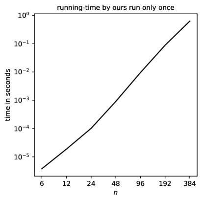
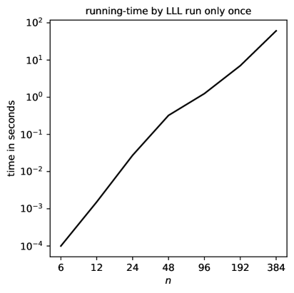
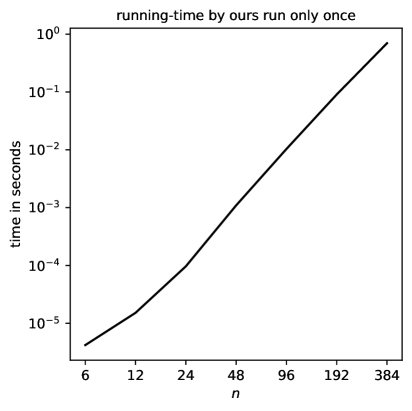
Figure 1: $\delta=1-10^{-15}$, $p=2$; the upper plots are for $q=2^{13}-1$, the lower plots are for $q=2^{31}-1$

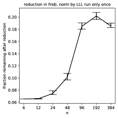
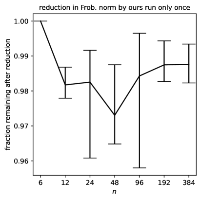
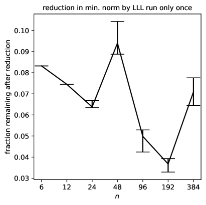
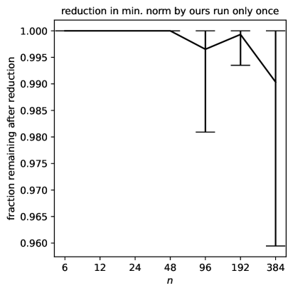
Figure 2: $\delta=1-10^{-15}$, $p=2$, $q=2^{13}-1$

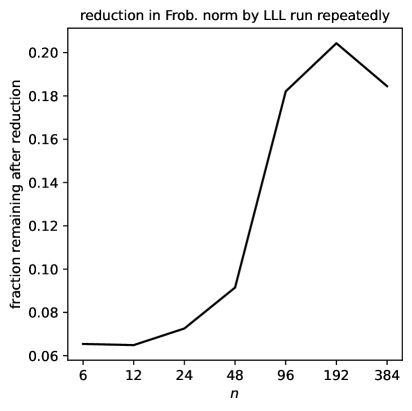
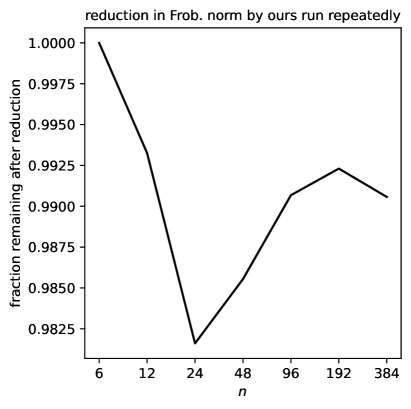
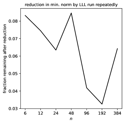
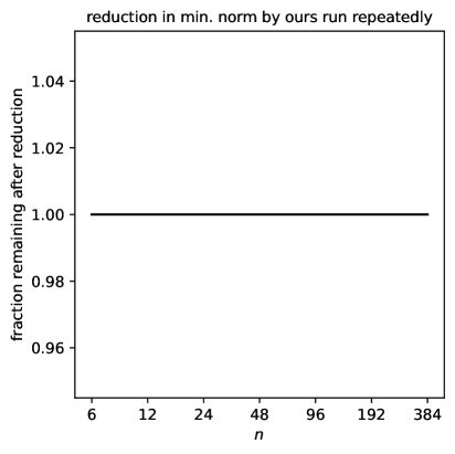
Figure 3: $\delta=1-10^{-15}$, $p=2$, $q=2^{13}-1$

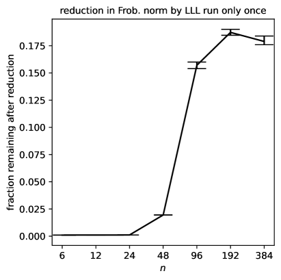
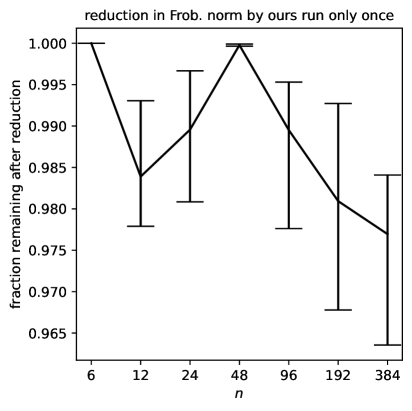
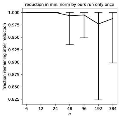
Figure 4: $\delta=1-10^{-15}$, $p=2$, $q=2^{31}-1$

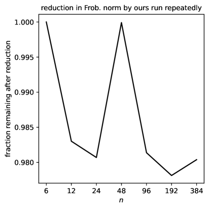
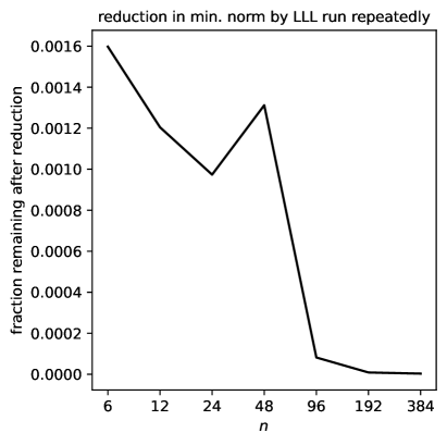
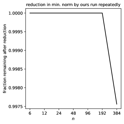
Figure 5: $\delta=1-10^{-15}$, $p=2$, $q=2^{31}-1$

4 Conclusion

The present paper proposes a very simple and efficient scheme for lattice reduction. The scheme reduces the Euclidean norms of the basis vectors monotonically, as guaranteed by rigorous proofs. Fortunately, the algorithm of the present paper runs much faster than even a highly optimized implementation of the most classical baseline, the LLL algorithm of Lenstra et al., (1982). Unfortunately, the proposed algorithm reduces norms far less than LLL if not used in conjunction with a method such as LLL. The main use of the proposed scheme should therefore be to polish the outputs of another algorithm (such as LLL). On its own, the algorithm of the present paper tends to get stuck in rather shallow local minima, with the iterations reaching an equilibrium that is far away from optimally minimizing the Euclidean norms of the basis vectors. Convergence is monotonic and hence guaranteed, but equilibrium tends to attain without reaching the global optimum. The algorithm of the present paper is extremely efficient computationally, however, so can be suitable for rapidly burnishing the outputs of other algorithms for lattice reduction.

Appendix A Poorly performing alternatives

This appendix mentions two possible modifications that lack the firm theoretical grounding of the algorithm presented above and performed rather poorly in numerical experiments. These modifications may be natural, yet seem not to work well. Subsection A.1 considers adding to a basis vector multiple other basis vectors simultaneously, such that the full linear combination would minimize the Euclidean norm if the coefficients in the linear combination did not have to be rounded to the nearest integers. Subsection A.2 considers a modified Gram-Schmidt procedure.

A.1 Combining multiple vectors simultaneously

One possibility is to choose a basis vector at random, say $a^{i}_{j}$, and add to that vector the linear combination of all other basis vectors which minimizes the Euclidean norm of the result, with the coefficients in the linear combination rounded to the nearest integers. That is, choose an index $j$ uniformly at random, and calculate real-valued coefficients $c^{i}_{j,k}$ such that the Euclidean norm $\|a^{i}_{j}-\sum_{k=1}^{n}c^{i}_{j,k}\cdot a^{i}_{k}\|$ is minimal, where $c^{i}_{j,j}=0$. Then, construct $a^{i+1}_{j}=a^{i}_{j}-\sum_{k=1}^{n}\operatorname{nint}(c^{i}_{j,k})\cdot a^{i}_{k}$.

Repeating the process for multiple iterations, $i=0$, $1$, $2$, …, would appear reasonable. However, this scheme worked well empirically only when the number $n$ of basis vectors was very small, at least when the number $m$ of entries in each of the basis vectors was equal to $n$. Rounding the coefficients $c^{i}_{j,k}$ to the nearest integers is too harsh for this process to work well.

A.2 Modified Gram-Schmidt process

Another possibility is to run the classical Gram-Schmidt procedure on the basis vectors, while subtracting off from all vectors not yet added to the orthogonal basis the projections onto the current pivot vector. In this modified Gram-Schmidt scheme, each iteration chooses as the next pivot vector the residual basis vector for which adding that basis vector to the orthogonal basis would minimize the sum of the $p$-th powers of the Euclidean norms of the reduced basis vectors. The iteration orthogonalizes the pivot vector against all previously chosen pivot vectors and then subtracts off (from all residual basis vectors not yet chosen as pivots) the projection onto the orthogonalized pivot vector, with the coefficients in the projections rounded to the nearest integers.

This scheme strongly resembles the LLL algorithm of Lenstra et al., (1982), but with a different pivoting strategy (using modified Gram-Schmidt). Numerical experiments indicate that the modified Gram-Schmidt performs somewhat similarly to yet significantly worse than the classical LLL algorithm. Omitting the bubble-sorting of the LLL algorithm via the so-called “Lovász criterion” spoils the scheme.

This scheme is also reminiscent of the variants of the LLL algorithm with so-called “deep insertions,” as developed by Schnorr & Euchner, (1994), Fontein et al., (2014), Yasuda & Yamaguchi, (2019), and others. LLL with deep insertions performs much better, however, both theoretically and practically. Other modifications to the LLL algorithm, notably the BKZ and BKW methods reviewed by Nguyen & Vallée, (2010) and others, also perform much better than the modified Gram-Schmidt.

Appendix B Further figures

This appendix presents figures analogous to those of Section 3, but using different values of the parameters $\delta$ and $p$ detailed in Subsection 3.1. Figures 6–10 are the same as Figures 1–5, but with $\delta=1-10^{-1}$ instead of $\delta=1-10^{-15}$. Figures 11–20 are the same as Figures 1–10 for $n=192$, but with varying values of $p$ rather than just $p=2$.

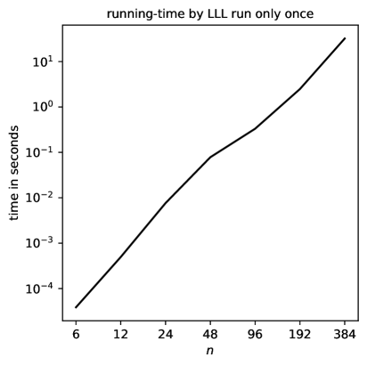
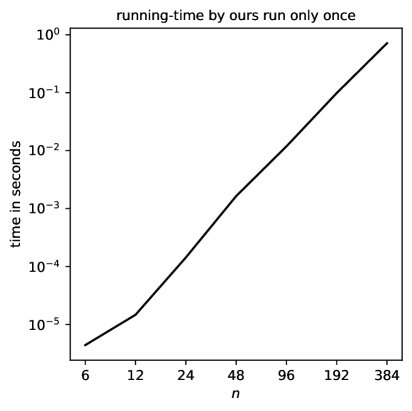
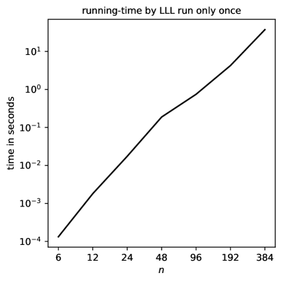
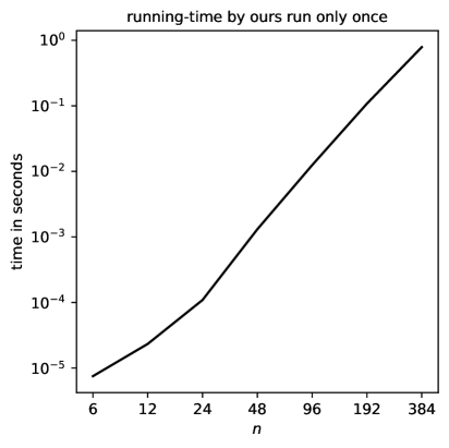
Figure 6: $\delta=1-10^{-1}$, $p=2$; the upper plots are for $q=2^{13}-1$, the lower plots are for $q=2^{31}-1$

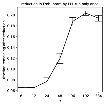
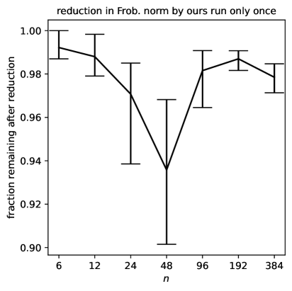
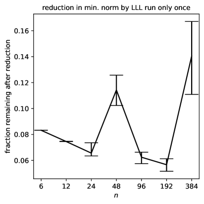
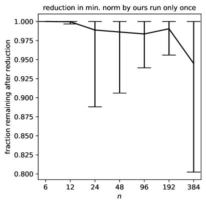
Figure 7: $\delta=1-10^{-1}$, $p=2$, $q=2^{13}-1$

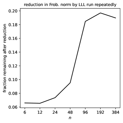
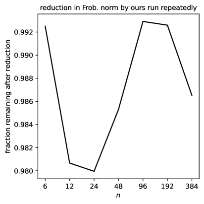
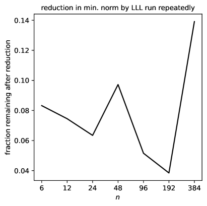
Figure 8: $\delta=1-10^{-1}$, $p=2$, $q=2^{13}-1$

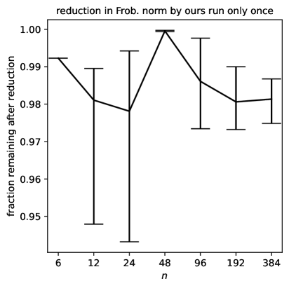
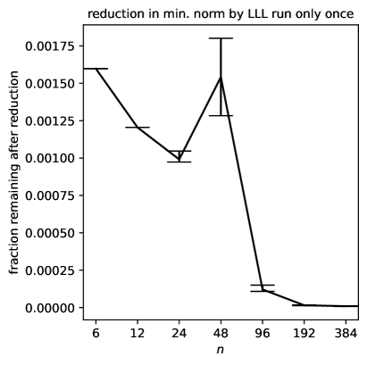
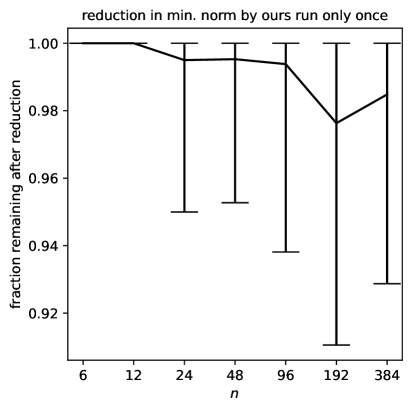
Figure 9: $\delta=1-10^{-1}$, $p=2$, $q=2^{31}-1$

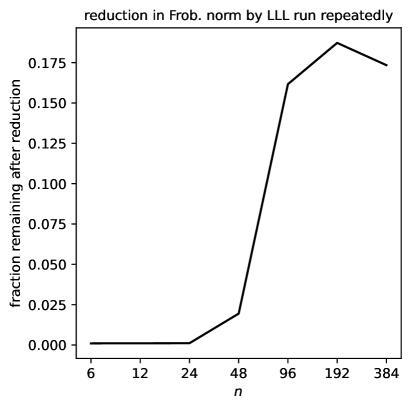
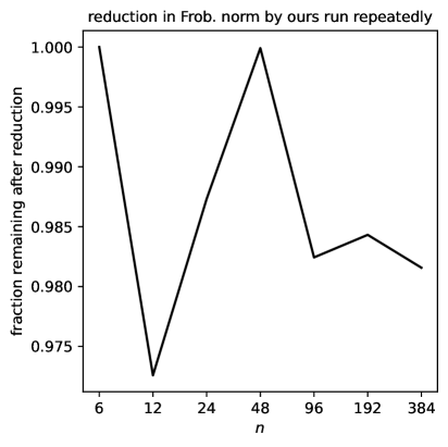
Figure 10: $\delta=1-10^{-1}$, $p=2$, $q=2^{31}-1$

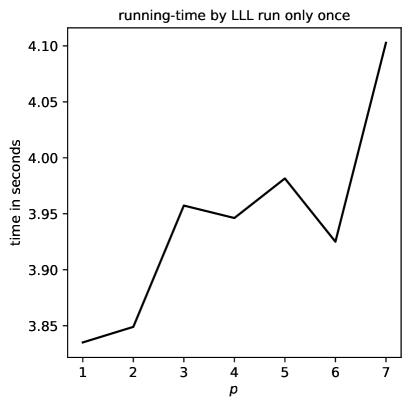
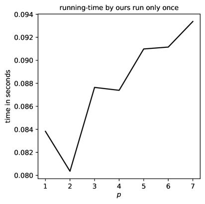
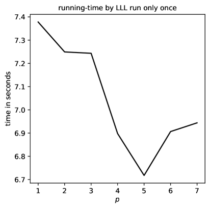
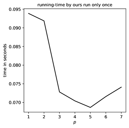
Figure 11: $\delta=1-10^{-15}$, $n=192$; the upper plots are for $q=2^{13}-1$, the lower plots are for $q=2^{31}-1$ … the vertical ranges of the plots on the left are very small, with the vertical variations displayed being statistically insignificant, wholly attributable to randomness in the computational environment.

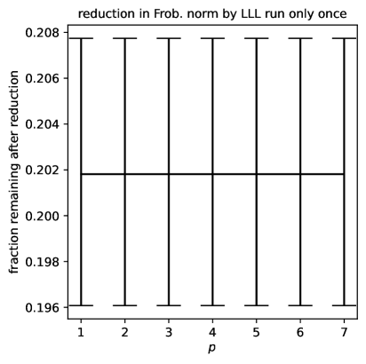
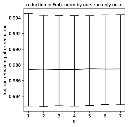
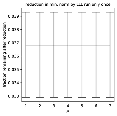
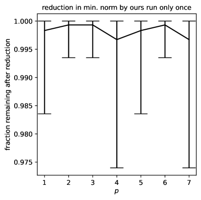
Figure 12: $\delta=1-10^{-15}$, $n=192$, $q=2^{13}-1$

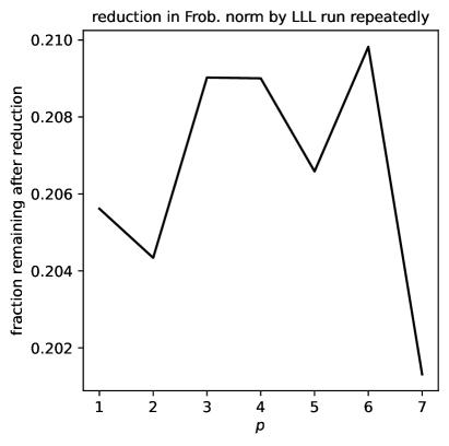
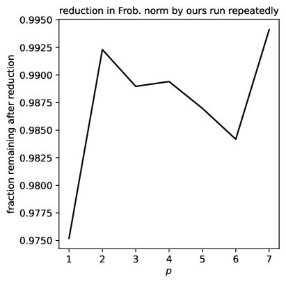
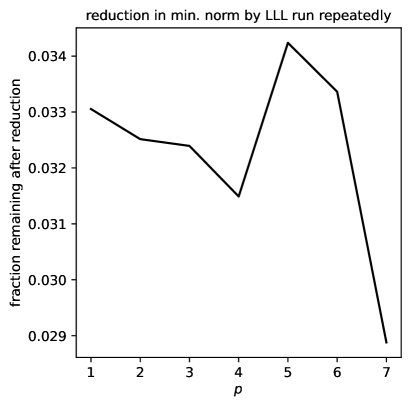
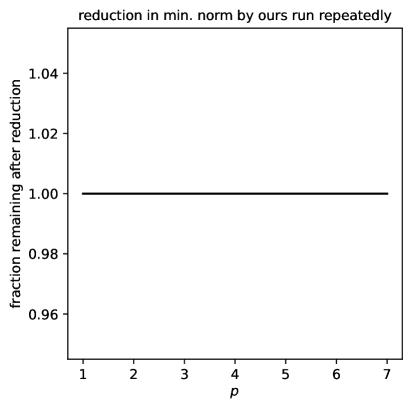
Figure 13: $\delta=1-10^{-15}$, $n=192$, $q=2^{13}-1$

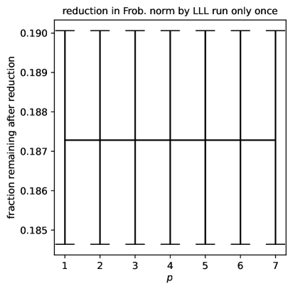
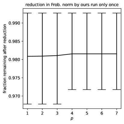
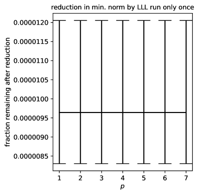
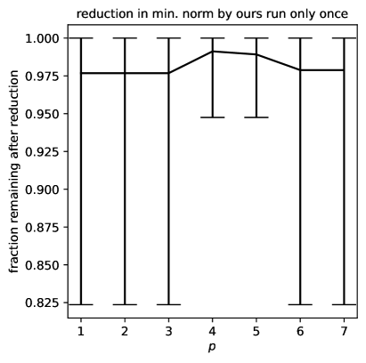
Figure 14: $\delta=1-10^{-15}$, $n=192$, $q=2^{31}-1$

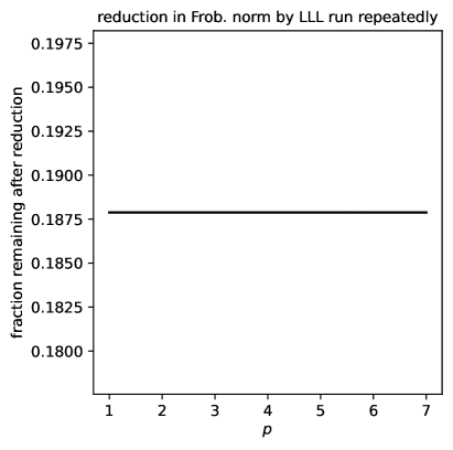
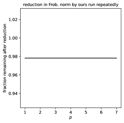
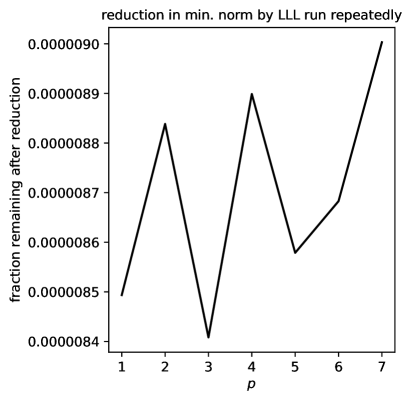
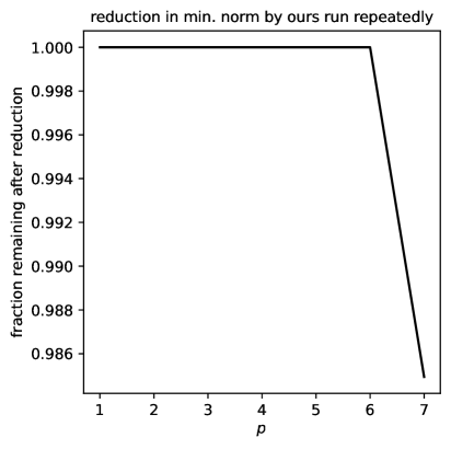
Figure 15: $\delta=1-10^{-15}$, $n=192$, $q=2^{31}-1$

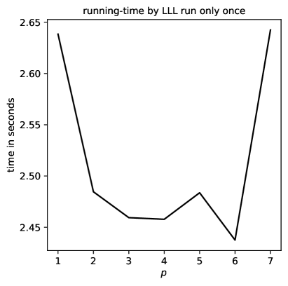
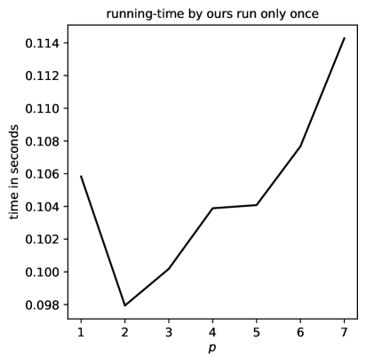
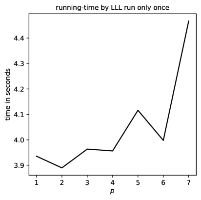
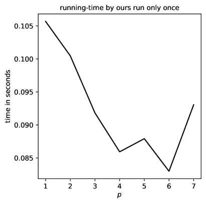
Figure 16: $\delta=1-10^{-1}$, $n=192$; the upper plots are for $q=2^{13}-1$, the lower plots are for $q=2^{31}-1$ … the vertical ranges of the plots on the left are very small, with the vertical variations displayed being statistically insignificant, wholly attributable to randomness in the computational environment.

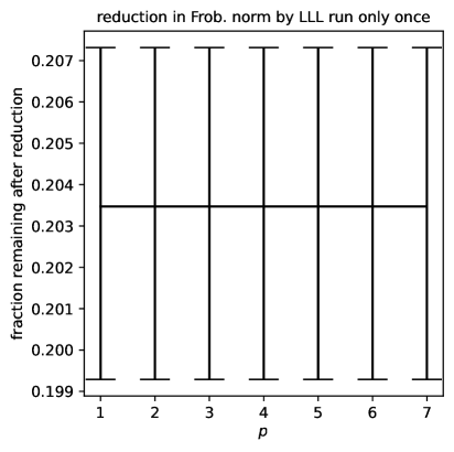
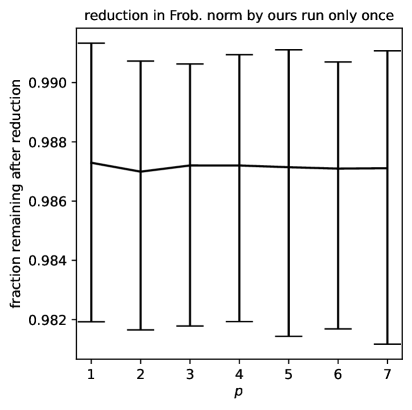
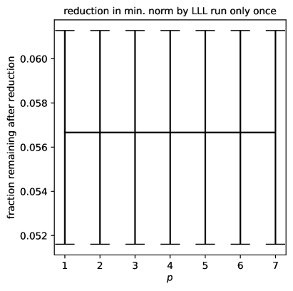
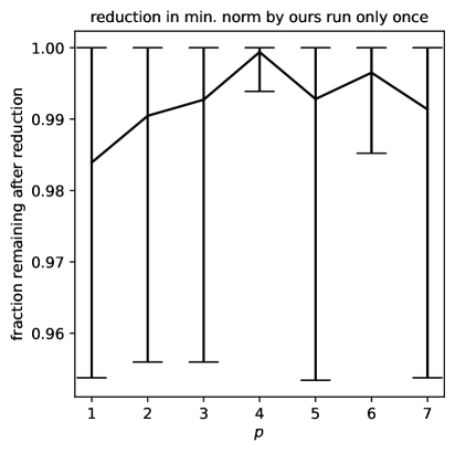
Figure 17: $\delta=1-10^{-1}$, $n=192$, $q=2^{13}-1$

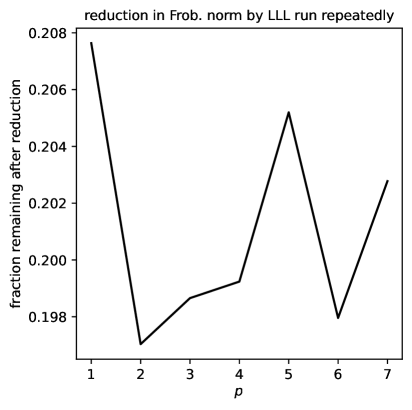
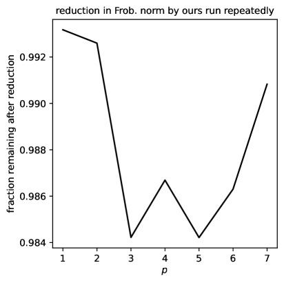
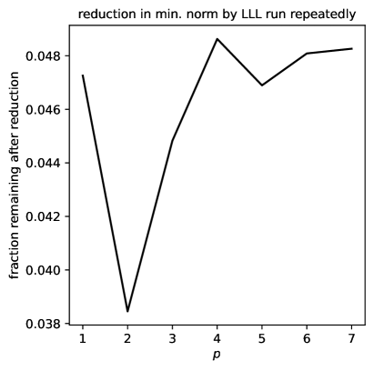
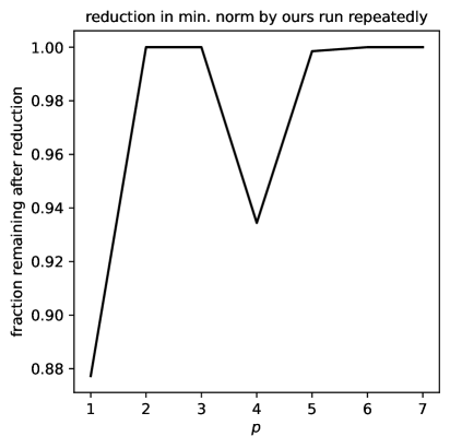
Figure 18: $\delta=1-10^{-1}$, $n=192$, $q=2^{13}-1$

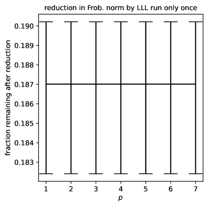
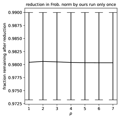
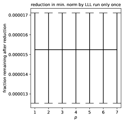
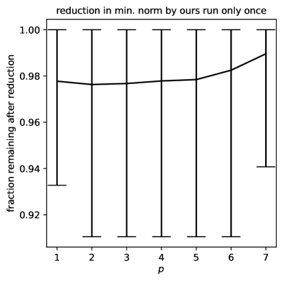
Figure 19: $\delta=1-10^{-1}$, $n=192$, $q=2^{31}-1$

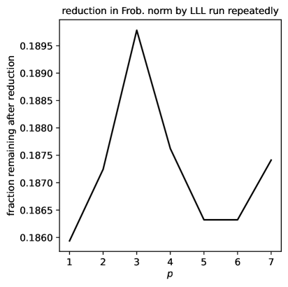
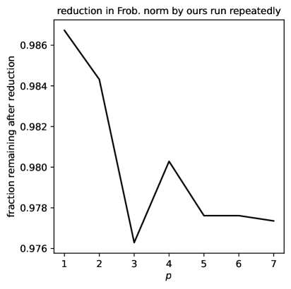
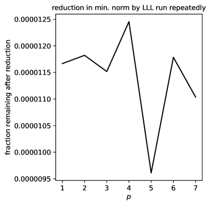
Figure 20: $\delta=1-10^{-1}$, $n=192$, $q=2^{31}-1$

References

- Banaszczyk, (1993) Banaszczyk, William. 1993. New bounds in some transference theorems in the geometry of numbers. Math. Ann., 296, 625–635.
- Blackford et al., (2002) Blackford, L. Susan, Demmel, James, Dongarra, Jack, Duff, Iain, Hammarling, Sven, Henry, Greg, Heroux, Michael, Kaufman, Linda, Lumsdaine, Andrew, Petitet, Antoine, Pozo, Roldan, Remington, Karin, & Whaley, R. Clint. 2002. An updated set of basic linear algebra subprograms (BLAS). ACM Trans. Math. Softw., 28(2), 135–151.
- Bremner, (2012) Bremner, Murray R. 2012. Lattice Basis Reduction: An Introduction to the LLL Algorithm and Its Applications. Pure and Applied Mathematics. Chapman & Hall, CRC Press.
- Cassels, (1997) Cassels, John William Scott. 1997. An Introduction to the Geometry of Numbers. Classics in Mathematics. Springer.
- Fontein et al., (2014) Fontein, Felix, Schneider, Michael, & Wagner, Urs. 2014. PotLLL: a polynomial time version of LLL with deep insertions. Des. Codes Cryptogr., 73, 355–368.
- Lawson et al., (1979) Lawson, Charles L., Hanson, Richard J., Kincaid, David, & Krogh, Fred T. 1979. Basic linear algebra subprograms for FORTRAN usage. ACM Trans. Math. Softw., 5(3), 308–323.
- Lenstra et al., (1982) Lenstra, Arjen K., Lenstra, Hendrik W., & Lovász, László. 1982. Factoring polynomials with rational coefficients. Math. Ann., 261(4), 515–534.
- Leon et al., (2013) Leon, Steven J., Björck, Åke, & Gander, Walter. 2013. Gram-Schmidt orthogonalization: 100 years and more. Numer. Lin. Algebra Appl., 20(3), 492–532.
- Nguyen & Vallée, (2010) Nguyen, Phong Q., & Vallée, Brigitte (eds). 2010. The LLL Algorithm: Survey and Applications. Information Security and Cryptography. Springer.
- Peikart, (2016) Peikart, Chris. 2016. A decade of lattice cryptography. Found. Trends Theor. Comput. Sci., 10(4), 283–424.
- Regev, (2009) Regev, Oded. 2009. On lattices, learning with errors, random linear codes, and cryptography. J. ACM, 56(6), 1–40.
- Schnorr & Euchner, (1994) Schnorr, Claus P., & Euchner, Martin. 1994. Lattice basis reduction: improved practical algorithms and solving subset sum problems. Math. Program., 66, 181–199.
- Stehlé, (2010) Stehlé, Damien. 2010. Floating-point LLL: theoretical and practical aspects. Pages 179–213 of: Nguyen, Phong Q., & Vallée, Brigitte (eds), The LLL Algorithm: Survey and Applications. Springer.
- Yasuda & Yamaguchi, (2019) Yasuda, Masaya, & Yamaguchi, Junpei. 2019. A new polynomial-time variant of LLL with deep insertions for decreasing the squared-sum of Gram-Schmidt lengths. Des. Codes Cryptogr., 87, 2489–2505.