RR Lyrae Visual to Infrared Absolute Magnitude Calibrations
In the light of Gaia DR3

Abstract

A probabilistic approach has been used in combination with the parallax data from Gaia (e)DR3 to calibrate Period-Luminosity-(Abundance) (PLZ) Relations covering a wide range of visual to Infrared observations of RR Lyrae stars. Absolute Magnitude Relations are given, derived from the same selection of stars, for $V$, $G$, $I$, $K_{\mathrm{s}}$ and WISE $W1$ as well as for for the reddening free pseudo-magnitudes $WBV$, $WVI$ and finally also Gaia $WG$. The classical relation between $M_{V}$ and $[\mathrm{Fe}/\mathrm{H}]$ is redetermined and as an illustration distances are given to a few selected objects.

Disclaimer: this paper reflects the presentation as given by J. Lub at the RRLCEP2022 conference (september 2022). Unfortunately after preparing this report we found out that only invited contributions would be published in the Proceedings.

1 Introduction

This talk is the fourth presentation in a series given at the RR Lyrae (and Cepheid) meetings initiated in 2015 at Visegrad (Lub, 2016, 2018, and 2021). The investigation started as an attempt to understand the origin of the $K$-$\log_{10}P$ relation and then to use this to improve absolute magnitude determinations in other photometric (visual) bands, taking advantage of the tightness of the PL(Z) relations and the reduced interstellar absorption in the infrared. In the meanwhile the incredible improvements of parallax, proper motion and photometric data (Gaia collaboration, 2016, 2018, 2021, 2022) have made it necessary to reconsider and extend the calibrations presented at Cloudcroft in 2019 (Lub, 2021). This progress is illustrated in Table 1. below. Much more is still to come.

It remains amusing, but not much more should be made out of this, to note how the parallax of RR Lyrae itself (in the last column) seems to increase as the precision of the determination increases with time.

Table 1: Time evolution of RR Lyrae parallaxes (units: milliarcseconds)

Source	year	$V_{\mathrm{average}}$	$\langle\varpi\rangle$	$\langle\sigma_{\varpi}\rangle$	$N_{\mathrm{sample}}$	$\varpi_{\mathrm{RRLyrae}}$	References
			mas	mas	$N_{\mathrm{sample}}$	mas
Hipparcos	1997 and 2007	11.09	0.992	3.193	143	3.46$\pm$ 0.64	1,2
HST	2011	9.21	2.16	0.16	5(4)	3.77$\pm$ 0.13	3
Gaia DR1	2016	11.13	0.938	0.312	132	3.64$\pm$ 0.23	4
Gaia DR2	2018	11.50	0.791	0.043	206	?	5
Gaia (e)DR3	2020 and 2022	11.50	0.824	0.021	207	3.985$\pm$ 0.027	6,7
Gaia DR4	(TBD)	11.50	-	0.010	207	-
Gaia DR5	(TBD)					Final catalogue

References: 1. Fernley et al. (1998), 2. Feast et al. (2008), 3. Benedict et al. (2011), 4,5,6 Brown et al. (2016), (2018), (2021), 7. Vallenari et al. (2022).

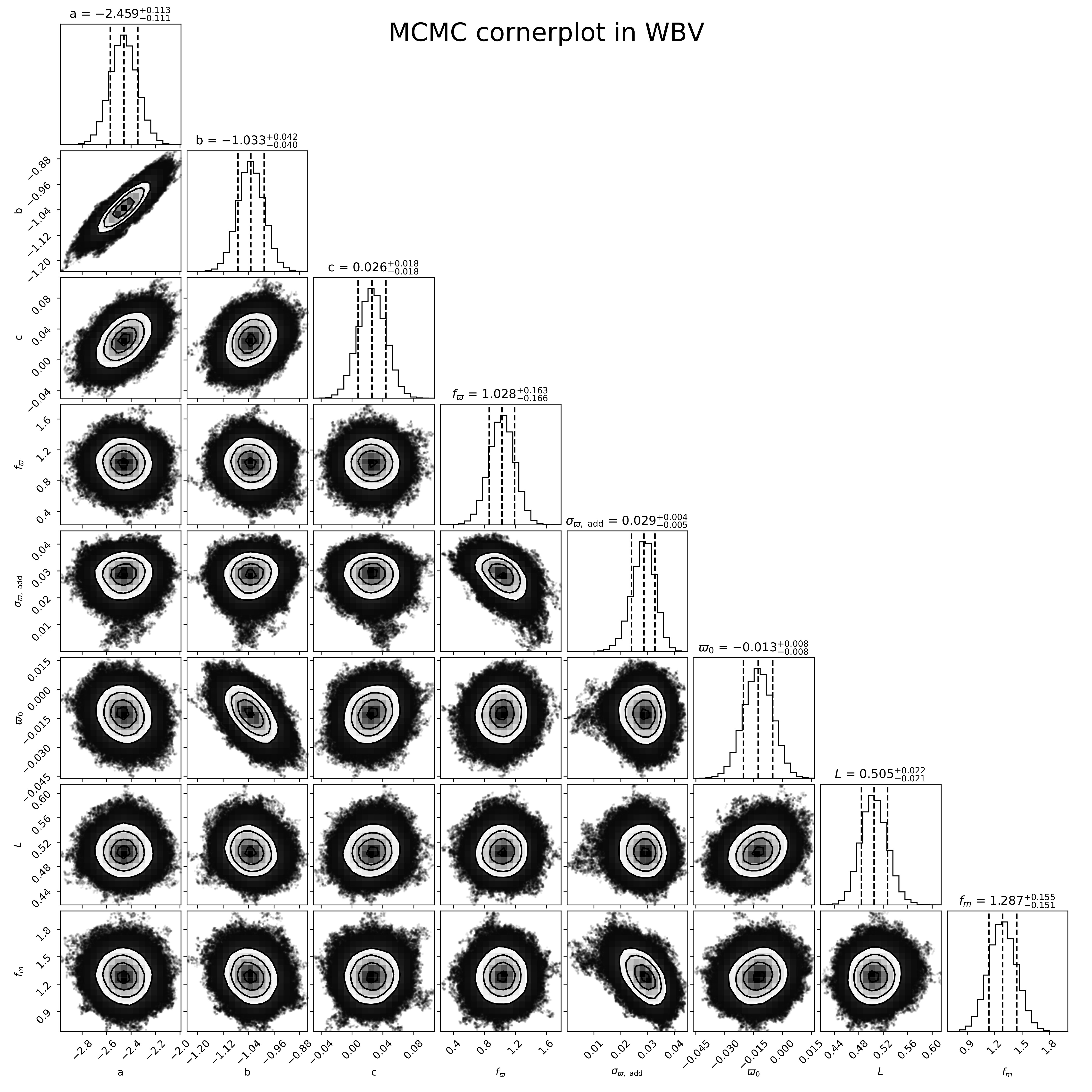
Figure 1: Cornerplot for $WBV$. Note that the coefficients $a$, $b$ and $c$ have been changed with respect to our definition to conform with the order in which they occur in Sesar et al. (2017)

2 Presentation of the RR Lyrae sample

Our sample of over 200 well studied RR Lyrae used before was updated with Gaia (e)DR3 parallaxes and photometry as well as W1 photometry. Monson et al. (2017) have discussed sample of 55 brighter RR Lyrae giving us the opportunity to also add also improved V and I photometry. Interstellar reddening and absorption were as before based on Schlafly and Finkbeiner (2011) with a simple correction for the pathlength within the galactic disk. An alternative approach in Muhie et al. (2021) is based upon their $V-K$ colours. After a comparison excluding stars too close to the galactic equator and obvious incorrect determinations (large negative absorptions from $V-K$) we could conclude that there was no offset beteeen the two methods.

RRc stars were fundamentalized by adding $0.1275$ to $\log_{10}P$  in conformity with the value derived from the three RRd stars in our sample and the results by Clementini et al. (2004) for M3. This gives as median values:

$$\log_{10}(P_{\mathrm{F}})=-0.28\,,\\ [\mathrm{Fe}/\mathrm{H}]=-1.38\,,\\ \langle V\rangle=11.50\,.$$

3 Estimating PLZ relations.

3.1 First approach

Our previous rather naive approach was to assume that in the PLZ relation:

$$M=a+b\log_{10}(P_{\mathrm{F}})+c([\mathrm{Fe}/\mathrm{H}]+1.35)$$

the coefficients $b$ and $c$ are as given by the 2015 Framework paper by Marconi et al. (2015). Ideally photometric parallaxes $\varpi_{\mathrm{phot}}$ based upon these PLZ relations can then be calculated from the fundamental relation:

$$(m-M)_{0}=-5\log_{10}(\varpi_{\mathrm{phot}})+10$$

where $m$ is the observed (pseudo)-magnitude and parallaxes are given in milliarcseconds. The coefficient a is then adjusted to give a one to one relation with respect to the Gaia parallaxes. The Gaia zeropoint offset then follows from the differences between the Gaia parallaxes and these so calculated photometric parallaxes. Our preliminary calibrations based upon Gaia DR2 presented in 2019 in Cloudcroft (Lub, 2021) were:

$$K_{\mathrm{s}}+2.25\log_{10}(P_{\mathrm{F}})=-1.055+0.18([\mathrm{Fe}/\mathrm{H}]+1.35)$$

$$WBV=\langle V\rangle_{\mathrm{int}}-3.06\langle B-V\rangle_{\mathrm{mag}}$$

$$=-1.035-2.49\log_{10}(P_{\mathrm{F}})$$

Whereas the Gaia DR2 zeropoint bias (see e.g. Lindegren et al., 2018) was found as $\varpi_{0}=-0.035\pm 0.010$ mas. Please note in the appendix the change in the definition of $WBV$ used in this work.

3.2 A probabilistic unbiased procedure to estimate PLZ relations.

It is clear that in this way no use is made of the full information available, as was pointed out almost immediately when Gaia DR1 (TGAS) became available, by Sesar et al. (2017). They introduced a probabilistic approach taking into count the full amount of information available in the data. Following their lead one of us (Koen Looijmans) undertook to set up and implement a procedure to allow for all measurement errors as well as a bias in the parallaxes $\varpi_{0}$ For the distance an exponentially decreasing volume density prior with a scale lenghth $L$ as proposed by Bailer-Jones (2015) was adopted.

As an example we show in Fig. 1 the corner plot for the pseudo magnitude $WBV$.

Table 2: Summary of MCMC solutions for PLZ relations in $W1$, $K_{\mathrm{s}}$, $V$ ,$WBV$, $I$ and $WVI$

Band	$a$	$b$	$c$	$\varpi_{0}$	$L$
				mas	kpc
$W1$	-1.153 $\pm$ 0.042	-2.53 $\pm$ 0.10	0.162 $\pm$ 0.016	-0.0189 $\pm$ 0.0080	0.502 $\pm$ 0.022
$K_{\mathrm{s}}$	-1.088 $\pm$ 0.043	-2.45 $\pm$ 0.11	0.171 $\pm$ 0.018	-0.0149 $\pm$ 0.0080	0.504 $\pm$ 0.022
$V$	0.393 $\pm$ 0.049	-0.82 $\pm$ 0.10	0.273 $\pm$ 0.022	-0.0137 $\pm$ 0.0091	0.506 $\pm$ 0.022
$WBV$	-1.033 $\pm$ 0.041	-2.46 $\pm$ 0.10	0.026 $\pm$ 0.018	-0.0127 $\pm$ 0.0076	0.505 $\pm$ 0.022
$I$	-0.115 $\pm$ 0.062	-1.22 $\pm$ 0.18	0.218 $\pm$ 0.025	-0.035 $\pm$ 0.019	0.325 $\pm$ 0.026
$WVI$	-1.063 $\pm$ 0.055	-2.47 $\pm$ 0.10	0.131 $\pm$ 0.031	-0.027 $\pm$ 0.016	0.327 $\pm$ 0.026

The coefficients $a$, $b$ and $c$ are called $M_{\mathrm{ref}}$, $a$ and $b$ respectively by Sesar et al. (2017), the quoted precisions are given by the average over the difference of the 84th and 16th percentile with the median

In the summary table (Table 2) the results for $V$ and $WVI$ are separated from the rest, because they derive from a different source with only 55 stars. The coefficient of the Period dependence in $W1$, $K_{\mathrm{s}}$, $WVI$ and $WBV$ are all very close to $-2.50$. This might at first look surprising, but removing the effect of the interstellar absorption also reduces at the same time the effect of temperature variations, making $WVI$ and $WBV$ very much like an infrared magnitude, mainly measuring the stellar angular diameter. The $I$ data also stand out because of a larger parallax offset $\varpi_{0}$, possibly because they are brighter stars.

4 Distance Determinations

Armed with our Period-Luminosity relations, we (re)derive the distances to selected globular clusters and the Large Magellanic Cloud as in Lub (2021). It should be kept in mind that pseudo-magnitudes suchs as WBV and WVI have the unfortunate property of increasing any calibration errors in the photometry. Errors are given as mean deviations of the mean.

First we discuss the Galactic Globular Clusters M3 and $\omega$ Cen, representative of the two Oosterhoff groups (OI and OII), with each over 150 RR Lyrae stars : M3 (NGC 5272) ($B$ and $V$ data Cacciari et al. 2005, $K_{\mathrm{s}}$ data Bhardwaj et al. 2020) and $\omega$ Cen (NGC 5139) ($B$, $V$ and $K_{\mathrm{s}}$ data Braga et al. 2016, 2018). M3 $WBV$ (all stars) $(m-M)_{0}=14.987$ ($\pm 0.059$) $K_{\mathrm{s}}$ (all stars) $15.047$ ($\pm 0.033$) $\omega$ Cen $WBV$ (all stars) $(m-M)_{0}=13.696$ ($\pm 0.012$) $K_{\mathrm{s}}$ (all stars) $13.720$ ($\pm 0.004$) Unfortunately in $\omega$ Cen our preliminary result from $WVI$ falls short: $(m-M)_{0}=13.578$ ($\pm 0.009$). This discrepancy remains for the moment unexplained.

In the Large Magellanic Cloud two fields, A and B, were studied in detail by Clementini et al. (2003), di Fabrizio et al. (2005), and Gratton et al. (2004), giving $BVI$ lightcurves and abundances. Proceeding as before in Cloudcroft We derive a distance modulus $(m-M)_{0}$ of $18.539$ ($\pm 0.017$) for field A and $18.504$ ($\pm 0.017$) for field B. The I measurements are unfortunately very much noisier and will not be discussed any further here. For these same two fields, $K$ measurements were added by Muraveva et al. (2015). More data are by Szewczyk et al. (2008) and Borissova et al. (2009) for stars in the general LMC field. We derive respectively in the same order: $18.584$ for field A, $18.548$ for field B, and $18.517$ and $18.485$ for the general field samples respectively. Errors of the median are of order $\pm 0.018$. Recently Cusano et al. (2021) collected tens of thousands of stars with $K_{\mathrm{s}}$ measurements and assuming an average $[\mathrm{Fe}/\mathrm{H}]=-1.50$ we find directly $(m-M)_{0}=18.561\pm 0.052$. But this needs further investigation.

5 The $M_{V}$ vs $[\mathrm{Fe}/\mathrm{H}]$ relation

The slope of the trend of absolute magnitude with metal abundance $[\mathrm{Fe}/\mathrm{H}]$ in the local RR Lyrae population was once a contentious issue, e.g. Sandage (1993), who advocated for a slope larger than $0.30$. However this appeared to have been settled to a value closer to $0.20$, based upon the discussion of LMC data by Gratton et  al. (2004). Unfortunately they did not cover a complete range of abundances. As discussed in Lub (2016, 2018, 2021), application the $K$-$\log_{10}P$ relation (and also the $WBV$-$\log_{10}P$ relation) directly leads back to the conclusion favoured by Sandage. By calculating the absolute magnitudes with the parallaxes from the $K$-$\log_{10}P$ and the $WBV$ calibrations, the afore mentioned relation becomes (see also Muraveva et al. 2018):

$$M_{V}=0.624(\pm 0.008)+0.334(\pm 0.015)([\mathrm{Fe}/\mathrm{H}]+1.35)$$

A mean value of $M_{V}=0.60$ has of course been in use for a long time.

6 Gaia magnitudes: $WG$

The photometry from the Gaia Satellite was originally not considered for this research. The reason for this was the fact that the published data are derived as straight means over the measured intensities, without reference to their phase in the lightvariation. However it clear as is true for WBV the combination from the Gaia magnitudes $G$, $G_{\mathrm{BP}}$ and $G_{\mathrm{RP}}$, viz.

$$WG=G-1.85(G_{\mathrm{BP}}-G_{\mathrm{RP}})$$

is a reddening free pseudo-magnitude derived from simultaneously measured intensities, which will reduce the lightcurve amplitude in a similar way as for $WBV$.

This is indeed borne out by comparing $WG$ with $W1$,$K_{\mathrm{s}}$ and $WBV$. Somehow taking out most of the temperature dependence gives rise to a kind of pseudo IR magnitude mainly dependent on the angular diameter as mentioned before. Apart from having a slope indistinguishable from one the median scatter is $0.043$, $0.056$ and $0.072$ (rms differences $0.056$, $0.073$ and $0.102$) respectively. This is indicative of the precision of the photometric measurements, where apparently W1 is superior.

As a shortcut we have used our calibrations for $WBV$ and $K_{\mathrm{s}}$ to predict each stars’ photometric parallax and taking the average value. A simple least squares approach, which of course then no longer takes into account the actually measured uncertanties and priors in the full probablistic approach the gives us:

$$WG=-1.093-2.475\log_{10}(P_{\mathrm{F}})+0.121([\mathrm{Fe}/\mathrm{H}]+1.35)$$

The errors on the coefficients are respectively: $0.020$, $0.065$ and $0.010$ and with this choice of $WG$ the Gaia DR3 zeropoint bias $\varpi_{0}$ comes out as $-0.008$ with an rms of $0.045$ ($0.0032$ for the median). A comparison with the separate investigation of Garofalo et al. (2022) shows very good agreement for coeficients and zeropoint.

It will be of interest to see how the full Bayesian approach will change this result when it is finally done. At any rate this calibration is fully consistent with our results for the other bands.

7 Conclusions

Gaia has set the zeropoint of the RR Lyrae Period-Luminosity relations with great precision. Here we have presented a set of Period-Luminosity-(Abundance) relations, which are internally consistent over the range fom $V$ to $W1$, because they are based on the same stellar sample. With only a few variables very good distances can de determined to all objects in the Local Group, which contain RR Lyrae stars.

Appendix A Intensity versus magnitude averages.

RR Lyrae stars have large $V$ amplitudes up till $1.25$ mag for RRab stars. The ratios between Blue ($B$) and near Infrared ($I$) amplitudes $Ab$ and $Ai$ to $V$ amplitude $Av$ are $1.29$ and $0.63$ respectively. Published data are a mixture of mean intensity converted to magnitude and average magnitude. Sometimes even intensity ratios are averaged. From our large collection of fully covered lightcurves (Lub, 1977) we derived :

$$\langle V\rangle_{\mathrm{int}}-\langle V\rangle_{\mathrm{mag}}=-0.047Av^{2}$$

The $B$ and near infrared $I$ lightcurves are very similar to the $V$ lightcurves so we can just substitute $Ab=1.29Av$ or $Ai=0.63Av$ for $Av$.

$$(\langle B\rangle_{\mathrm{int}}-\langle V\rangle_{\mathrm{int}})-(\langle B\rangle_{\mathrm{mag}}-\langle V\rangle_{\mathrm{mag}})=-0.031Av^{2}$$

$$(\langle V\rangle_{\mathrm{int}}-\langle I\rangle_{\mathrm{int}})-(\langle B\rangle_{\mathrm{mag}}-\langle V\rangle_{\mathrm{mag}})=-0.027Av^{2}$$

In this way also different definitions of the pseudo magnitude WBV can be related. However since our earlier work we have changed the definition of $WBV$ to conform with Neeley et al. (2019) replacing the absorption correction with 3.128 instead of 3.06, viz.

$$WBV=\langle V\rangle_{\mathrm{int}}-3.128\langle B-V\rangle_{\mathrm{mag}}$$

because we consider $\langle V\rangle_{\mathrm{int}}$ a good estimate of the bolometric luminosity and $\langle B-V\rangle_{\mathrm{mag}}$ a better temperature indicator than the intensity average. However over our sample the mean of $Av^{2}=0.980$ so using the definition of $WBV$ preferred by Marconi et al. would cause a positive shift of 0.094 in the zeropoint of the WBV relation. Lightcurve amplitudes are increasing towards shorter periods. After some experiments we have concluded that this increases the slope when only RRab stars are considered in deriving the PLZ relation. The coefficient of the period dependence increasing from close to $-2.5$ to $-2.75$.

For $WVI$ and also for Gaia $G$, $G_{\mathrm{BP}}$ and $G_{\mathrm{RP}}$ we have prefered to use the published intensity means:

$$WVI=\langle I\rangle_{\mathrm{int}}-1.38(\langle V\rangle_{\mathrm{int}}-\langle I\rangle_{\mathrm{int}})$$

$$WG=\langle G\rangle_{\mathrm{int}}-1.85(\langle G_{\mathrm{BP}}\rangle_{\mathrm{int}}-\langle G_{\mathrm{RP}}\rangle_{\mathrm{int}})$$

References

- Arenou et al. (2018) Gaia Collaboration; Arenou, F. , et al. 2018, A&A, 616, A17
- Bailer-Jones (2015) Bailer-Jones, C.A.L. 2015, PASP 127,994
- Benedict et. al (2011) Benedict, G.F. et al. 2011, AJ, 142, 187
- Bhardwaj et al. (2020) Bhardwaj, A. et al. 2020, AJ 160, 220
- Borissova et al. (2009) Borissova, J. et al. 2009, A&A. 502, 505
- Braga et al. (2016) Braga, V.F. et al. 2016, AJ ,152, 170
- Braga et al. (2018) Braga, V.F. et al. 2018, AJ ,155, 137
- Brown et al. (2016) Gaia Collaboration; Brown, A., et al 2016, A&A, 595, 2
- Brown et al. (2018) Gaia Collaboration; Brown, A., et al 2018, A&A, 616, A1
- Brown et al. (2021) Gaia Collaboration; Brown, A., et al 2021, A&A, 649, A1
- Cacciari et al. (2005) Cacciari, C. et al. 2005, AJ, 129, 267
- Clementini et al. (2003) Clementini, G., Gratton, R.G., Bragaglia, A. et al. 2003, AJ, 125, 1309
- Clementini et al. (2004) Clementini, G. et al. 2004, AJ, 127, 938
- Corwin et al. (2008) Corwin, T.M., et al. 2008, AJ ,135, 1459
- Dambis et al. (2013) Dambis, A.K. et. al 2013, MNRAS, 435, 230
- Di Fabrizio et al. (2005) Di Fabrizio, L. et. al 2005, A&A, 430, 603
- Feast et al. (2008) Feast, M.W, Laney, C.D. Kinman T.D. et al 2008 MNRAS 386,211
- Fernley et al. (1998) Fernley, J., Barnes, T.G., Skillen, I., et al. 1998, A&A, 330, 515
- Garofalo et al. (2022) Garofalo, A. et al 2022, MNRAS 513,788
- Gratton et al. (2004) Gratton, R.G., Bragaglia, A., Clementini, G., et al. 2004, A&A, 421, 937
- Lindegren et al. (2018) Lindegren, L. , et al. 2018, A&A, 616, A2
- Lub (2016) Lub, J. 2016, in: RRL2015: High Precision Studies of RR Lyrae Stars, Eds. L. Szabados, R. Szabo, K. Kinemuchi, Co. Kon., 105, 39
- Lub (2018) Lub, J. 2018, in: RRL2017: The Revival of the Classical Pulsators, Eds. R. Smolec, K. Kinemuchi, R.I. Anderson, Proc. Polish Astron. Soc. 6, 176
- Lub (2021) Lub, J. 2021, in: RRL/Cepheid2019: Frontiers of Classical Pulsators, Eds. K. Kinemuchi, C Lovekin, H. Neilson and K.Vivas, ASP Conf. Series 529, 22
- Marconi et al. (2015) Marconi, M. et. al 2015, ApJ, 808, 50
- Monson et al (2017) Monson, A.J. et al 2017 AJ 153,96
- Muhie et al (2021) Muhie, T.D. et al 2021, MNRAS 502,407
- Muraveva et al (2015) Muraveva, T., Walker, M., Clementini, G., et al. 2015, ApJ, 807, 127
- Muraveva et al. (2018) Muraveva, T., Delgado, H.E., et al. 2018, MNRAS, 481, 1195
- Neeley (2019) Neeley, J.R. , Marengo, M. et al 2019, MNRAS 490,425
- Sandage (1993) Sandage, A.R. 1993, AJ , 106, 703
- Schlafly&Finkbeiner (2011) Schlafly, E.M., Finkbeiner, D.S. 2011, ApJ, 737, 310
- Sesar et al. (2017) Sesar, B., Fourneau, M., et al. 2017, ApJ, 838,107
- Szewczyk et al. (2008) Szewczyk, O., et al. 2008, AJ , 136, 272
- Vallenari et al. (2022) Gaia Collaboration; Vallenari, A., et al. 2022 ,2022ArXiv22080021G