Large-scale simulations of Floquet physics on near-term quantum computers

Abstract

Quantum systems subject to periodic driving exhibit a diverse set of phenomena both of fundamental and technological interest. However, such dynamical systems are more challenging to simulate classically than their equilibrium counterparts. Here, we introduce the Quantum High Frequency Floquet Simulation (QHiFFS) algorithm as a method for simulating the dynamics of fast-driven Floquet systems on quantum hardware. Central to QHiFFS is the concept of a kick operator which transforms the system into a basis where the dynamics is governed by a time-independent effective Hamiltonian. This allows prior methods for time-independent Hamiltonian simulation to be lifted to the simulation of Floquet systems. We use the periodically driven biaxial next-nearest neighbor Ising (BNNNI) model as a case study to illustrate our algorithm. This oft-studied model is a natural test bed for quantum frustrated magnetism and criticality. We successfully implemented a 20-qubit simulation of the driven two-dimensional BNNNI model on Quantinuum’s trapped ion quantum computer. This is complemented with an analysis of QHiFFS algorithmic errors. Our study indicates that the algorithm exhibits not only a cubic scaling advantage in driving frequency $\omega$ but also a linear one in simulation time $t$ compared to Trotterisation, making it an interesting avenue to push towards near-term quantum advantage.

I Introduction

Figure 1: Method overview. (a) QHiFFS Algorithm Concept. To realize a time-dependent periodic time evolution, we transform from the standard basis to a (periodically) rotating frame using $e^{+i\hat{K}(t_{0})}$. Evolution in this frame from $t_{0}$ to $t$ is governed by the time-independent effective Hamiltonian $\hat{H}_{\mathrm{eff}}$. The adjoint of the kick operator $e^{-i\hat{K}(t)}$ is applied at the final simulation time $t$ to kick back into the original frame. (b) Benchmark system. To demonstrate the advantage of QHiFFS, as compared to standard Trotterization, we implement the 20-qubit transversely driven 2D biaxial next-nearest neighbor Ising (BNNNI) model with periodic boundary conditions on Quantinuum’s H1 trapped ion quantum hardware (see Fig. 3). The BNNNI model, Eq. (8), consists of nearest-neighbour coupling with strength $J$ and next-nearest-neighbour coupling with strength $\kappa J$. We suppose a 4 by 5 qubit lattice is periodically driven with strength $h$ and at frequency $\omega$.

There has been a recent spike of interest in the dynamical control of quantum phases by driving strongly correlated quantum systems out of equilibrium. In particular, Floquet systems, that is quantum systems subjected to periodic driving, not only exhibit a rich set of physical phenomena, including exotic non-equilibrium topological phases of matter Rudner et al. (2013); Khemani et al. (2016); Moessner and Sondhi (2017); Else et al. (2017); Martin et al. (2017); Moessner and Moore (2021), but can also generate quantum phenomena on demand for technological applications Lindner et al. (2011); Mentink et al. (2015); Mitrano et al. (2016); Basov et al. (2017); McIver et al. (2020). For example, time crystalline phases Wilczek (2012), which break continuous time-translational symmetry have been demonstrated with trapped ions Zhang et al. (2017), superconducting qubits Ippoliti et al. (2021); Mi et al. (2022); Frey and Rachel (2022) and diamond defects Randall et al. (2021). Similarly, periodic driving can lead to symmetry-protected edge modes Khemani et al. (2016); Potter et al. (2016); Moessner and Sondhi (2017); Moessner and Moore (2021), a phenomenon that has been realized in both trapped ions Dumitrescu et al. (2022) and superconducting Zhang et al. (2022) platforms, and has potential applications for error correction. However, the strong correlations present in such systems make their modelling classically challenging.

The potential of simulating the dynamics of quantum systems exponentially more efficiently than is possible classically provided one of the original motivations for developing quantum hardware Feynman (1982); Schuch et al. (2008); Wolf (2006). While a distant dream for decades, with rapid technological progress, the possibility of realising a quantum advantage for quantum simulation is now in sight Arute et al. (2019); Zhong et al. (2020). Nonetheless, error rates are yet to reach the error correction threshold for moderate-sized devices and hence quantum simulation algorithms designed for fault-tolerant devices remain challenging for the near future Lloyd (1996); Sornborger and Stewart (1999); Verstraete et al. (2009); Berry et al. (2015); Low and Chuang (2019). This has prompted the search for quantum simulation algorithms suitable for implementation on near-term quantum devices Verstraete et al. (2009); Cirstoiu et al. (2020); Gibbs et al. (2021, 2022); Mansuroglu et al. (2021); Kökcü et al. (2021); Trout et al. (2018); Endo et al. (2020); Yao et al. (2021); Otten et al. (2019); Benedetti et al. (2020); Barison et al. (2021); Bharti and Haug (2021); Lau et al. (2021). However, most of these studies focused on simulating time-independent systems and less attention has so far been paid to how to simulate periodically driven systems.

Standard Trotterization Rudner et al. (2013); Khemani et al. (2016); Moessner and Sondhi (2017); Else et al. (2017); Martin et al. (2017); Moessner and Moore (2021); Potter et al. (2016); Dumitrescu et al. (2022); Zhang et al. (2022); Wilczek (2012); Zhang et al. (2017); Ippoliti et al. (2021); Mi et al. (2022); Frey and Rachel (2022); Randall et al. (2021); Schneider and Saenz (2012); Fauseweh and Zhu (2021a, b); Lamm and Lawrence (2018); Oftelie et al. (2020); Rodriguez-Vega et al. (2022), where the time-ordered integral governing the dynamics is discretized into short time-steps (implemented via a Trotter approximation), fails to take advantage of the periodic structure of Floquet problems and thus acquires a substantial computational overhead. Alternative proposals include solving the Schrödinger-Floquet equation Fauseweh and Zhu (2021b); Mizuta and Fujii (2022) and using variational optimization Lamm and Lawrence (2018). The former requires fault-tolerant techniques and the latter is limited by (noise-induced) barren plateaus McClean et al. (2018); Cerezo et al. (2021); Holmes et al. (2022, 2021); Patti et al. (2021); Marrero et al. (2021); Arrasmith et al. (2022); Wang et al. (2021) as well as other barriers to variational optimization on near-term quantum hardware Bittel and Kliesch (2021); Rivera-Dean et al. (2021); Anschuetz and Kiani (2022). Correspondingly, digital quantum simulations of systems subject to a continuous driving field have thus far been limited to only a few qubits Oftelie et al. (2020); Rodriguez-Vega et al. (2022).

Here we draw motivation from prior work on classical methods for studying Floquet physics Floquet (1883); Magnus (1954); Shirley (1965); Goldman and Dalibard (2014); Eckardt and Anisimovas (2015); Bukov et al. (2015); Oka and Kitamura (2019) and methods for analogue quantum simulation Schneider and Saenz (2012), to develop a new quantum algorithm for simulating periodically driven systems on digital quantum computers. Crucially this approach takes explicit advantage of the periodicity of the driving terms to reduce the resource requirements of the simulation. Key to our approach, is the use of a high-frequency approximation that performs a time-dependent basis transformation into a rotating frame Goldman and Dalibard (2014). This transformation, which can be implemented on quantum hardware using a kick operator, allows one to transform a time-dependent quantum simulation into a time-independent one. Previously developed time-independent techniques can then be lifted and reused for the Floquet simulation Lloyd (1996); Sornborger and Stewart (1999); Verstraete et al. (2009); Berry et al. (2015); Low and Chuang (2019); Cirstoiu et al. (2020); Gibbs et al. (2021); Mansuroglu et al. (2021); Gibbs et al. (2022); Kökcü et al. (2021). The Quantum High Frequency Floquet Simulation (QHiFFS – pronounced quiffs) algorithm thus opens up the potential of simulating fast-driven systems using substantially shorter-depth circuits than standard Trotterisation.

We use QHiFFS to implement a 20-qubit two-dimensional simulation of the transversely driven biaxial next-nearest neighbor Ising (BNNNI) model on a trapped ion quantum computer. This implementation is, to the best of our knowledge, the largest digital 2D quantum simulation of a periodically driven system to date (see Sec. III). We choose to focus on the BNNNI model because it is one of the most representative spin-exchange models containing both tunable frustration and tunable quantum fluctuations, creating competing quantum phases and criticality. Indeed, this behaviour is successfully captured by our hardware implementation. We stress that this simulation would not have been feasible using standard Trotterisation, which would have required a 50-fold deeper circuit (see Fig. 3).

Finally, we set QHiFFS on solid analytic foundations by providing an analysis on the scaling of the final simulation errors. In particular, we find that first order QHiFFS not only exhibits a cubic scaling advantage in driving frequency $\omega$, but also a linear one in simulation time $t$ compared to a second order Trotter sequence. The scaling in system size $n$ remains linear for local models (see Sec. III.3). Thus we see QHiFFS finding use both on moderate-sized error-prone near-term devices and in the fault tolerant era.

II The QHiFFS Algorithm

The QHiFFS algorithm simulates quantum systems governed by a Hamiltonian of the form

$$\hat{H}(t)=\hat{H}_{0}+\hat{V}(t)\quad\mathrm{with}\quad\hat{V}(T+t)=\hat{V}(t)\,,$$ (1)

where $\hat{H}_{0}$ is the time independent non-driven Hamiltonian and $\hat{V}(T+t)$ is a periodic driving term. Without loss of generality the driving term can be expanded in terms of its Fourier components $\hat{V}^{(j)}$ as

$$\hat{V}(t)=\sum_{j=1}^{\infty}\hat{V}^{(j)}e^{ij\omega t}+\hat{V}^{(-j)}e^{-ij\omega t}\,.$$ (2)

where $\omega=2\pi/T$ is the driving frequency. Here we focus on the limit where the driving frequency is large, that is (in broad terms) when $\omega\gg||\hat{H}_{0}||_{\infty}$ and $\omega\gg||\hat{V}_{j}||_{\infty}$. Our aim is to simulate real time evolution under this Hamiltonian from some initial time $t_{0}$ to some final time $t$. That is, to implement the unitary

$$\hat{U}_{\rm exact}(t_{0},t) =\mathcal{T}\exp\left(-i\int_{t_{0}}^{t}\hat{H}(t)dt\right)\,,$$ (3)

where $\mathcal{T}$ is the time ordering operator.

As is often found in physics, choosing the right reference frame is key to a simple description of the dynamics of a system. To take a paradigmatic example - the motion of planets in our solar system appears rather complex in the earth’s reference frame but becomes much simpler if we transform into the frame of reference of the sun. Our algorithm, as sketched in Fig. 1, takes a similar approach Whaley and Light (1984); Rahav et al. (2003). Namely, we use a time-dependent kick operator, $\hat{K}(t)$, to transform the system to a frame of reference where the dynamics of the driven system is governed by a time-independent effective Hamiltonian, $\hat{H}_{\rm eff}$.

More concretely, the total simulation is composed of the following steps:

1. We apply $e^{+i\hat{K}(t_{0})}$ to kick an initial state $|\psi\rangle$ at time $t_{0}$ into our preferred reference frame.

2. We apply $e^{-i(t-t_{0})\hat{H}_{\rm eff}}$ to evolve the state from times $t_{0}$ to $t$ in this new reference frame.

3. We apply $e^{-i\hat{K}(t)}$ to kick the system back into the original (lab) frame of reference.

Or, more compactly, the total simulation is of the form

$$\hat{U}_{\rm exact}(t_{0},t) =e^{-i\hat{K}(t)}e^{-i(t-t_{0})\hat{H}_{\rm eff}}e^{+i\hat{K}(t_{0})}\,.$$ (4)

Crucially, as previously claimed, $\hat{H}_{\rm eff}$ is time-independent. Thus, one can use prior methods Lloyd (1996); Sornborger and Stewart (1999); Verstraete et al. (2009); Berry et al. (2015); Low and Chuang (2019); Cirstoiu et al. (2020); Gibbs et al. (2021); Mansuroglu et al. (2021); Gibbs et al. (2022); Kökcü et al. (2021) for time-independent quantum simulation for its implementation. Furthermore, in many cases, as discussed below, the kick operator, $\hat{K}(t)$, will take a simple form enabling it to be easily implemented on quantum hardware.

The appropriate kick transformation and corresponding effective Hamiltonian for a periodically-driven system, Eq. (1), were derived in Ref. Goldman and Dalibard (2014) by expanding the kick operator and effective Hamiltonian in powers of the driving frequency as

$$\hat{K}(t)=\sum_{k=1}^{\infty}\frac{1}{\omega^{k}}\hat{K}^{(k)}(t)\quad\mathrm{and}\quad\hat{H}_{\rm eff}=\sum_{k=0}^{\infty}\frac{1}{\omega^{k}}\hat{H}_{\rm eff}^{(k)}\,.$$ (5)

As explained in detail in Appendix B.1, by first substituting Eq. (5) into Eq. (4) and effectively comparing with Eq. (3) (using Hadamard’s lemma), one can iteratively identify the terms $\hat{K}^{(k)}(t)$ and $\hat{H}_{\rm eff}^{(k)}$ by associating time-independent terms with $\hat{H}_{\rm eff}^{(k)}$ and time-dependent ones with $\hat{K}^{(k)}(t)$. In particular, truncating at $\mathcal{O}(\frac{1}{\omega^{2}})$, the effective Hamiltonian $\hat{H}_{\rm eff}$ and kick operator $\hat{K}(t)$ are given by:

$$\hat{H}_{\rm eff} \approx\hat{H}_{0}+\frac{1}{\omega}\sum_{j=1}^{\infty}\frac{1}{j}[\hat{V}^{(j)},\hat{V}^{(-j)}]$$ (6)

$$\hat{K}(t) \approx-\frac{i}{\omega}\sum_{j=1}^{\infty}\frac{1}{j}\left(\hat{V}^{(j)}e^{ij\omega t}-\hat{V}^{(-j)}e^{-ij\omega t}\right)$$ (7)

For expressions for $\hat{H}_{\rm eff}$ and $\hat{K}(t)$ at higher orders, see Appendix B. We note that the rotating wave approximation takes an analogous approach in the sense that under the rotating wave approximation evolution is governed by the $0^{\rm th}$ order approximation to the propagator in the interaction picture.

The resources required to implement a simulation via the QHiFFS algorithm depend on the forms of $\hat{V}(t)$ and $\hat{H}_{0}$. Here we describe a physically motivated setting in which the final simulation is particularly simple. A more detailed account of the resources required for other cases is included in Appendix B.2.

In what follows, we will focus on local driving (i.e., assume $\hat{V}(t)$ is one-local). This is a natural limit to consider since many driving phenomena, for example the optical driving of lattice systems, can be modeled in terms of local driving. In this case, $\hat{K}(t)$ is one-local to second order. Thus the initial and final kicks in Eq. (4) can be implemented using only single qubit rotations. If we further assume that $\hat{V}^{(j)}$ and $\hat{V}^{(-j)}$ commute for all $j$, which is the case here, then the first order correction to $\hat{H}_{\rm eff}$ vanishes and we have that $\hat{H}_{\rm eff}=\hat{H}_{0}+O(\frac{1}{\omega^{2}})$.

Within this setting (namely local driving with $\hat{V}^{(j)}$ and $\hat{V}^{(-j)}$ commuting), we have that to second order in $\frac{1}{\omega}$ the resources to simulate $\hat{H}_{\rm eff}$ are determined by the requirements for simulating $\hat{H}_{0}$. This is one of the main benefits of the QHiFFS algorithm. Namely, it allows one to reuse previously developed time-independent techniques and lift them to a Floquet Hamiltonian simulation Verstraete et al. (2009); Berry et al. (2015); Low and Chuang (2019); Cirstoiu et al. (2020); Gibbs et al. (2021); Mansuroglu et al. (2021); Gibbs et al. (2022). For example, if $\hat{H}_{0}$ is diagonal, or it can be analytically diagonalized, then one can simulate evolution under $\hat{H}_{\rm eff}$, and correspondingly evolution under $\hat{H}(t)$, using a fixed depth circuit. The transversely driven Ising model (independent of topology and dimension) falls into this category. More generally, one could use known methods for simulating the time-independent $1$D $XY$-model Verstraete et al. (2009), Bethe diagonalizable models Sopena et al. (2022) and translationally symmetric models Mansuroglu et al. (2021), to simulate the effect of local driving on such systems.

We note that in classical simulations of Floquet systems, high frequency expansions are known and commonly used Magnus (1954); Goldman and Dalibard (2014); Eckardt and Anisimovas (2015); Bukov et al. (2015); Oka and Kitamura (2019) both for simulation and for Floquet engineering. In the latter case, Eq. 3 and Eq. 4 are viewed from the opposite perspective to the one we take here. Namely, the time-dependent driving term, $\hat{V}(t)$, can be designed to implement otherwise unfeasible complex many-body time-independent Hamiltonians, $\hat{H}_{\rm eff.}$. This perspective is also taken in the quantum computing community for gate calibration and optimisation Sameti and Hartmann (2019); Petiziol et al. (2021); Qiao et al. (2021). However, on digital quantum computers the harder task is typically to simulate the time-ordered integral. Hence, this is our focus here. Namely, we propose implementing Eq. (4) on quantum hardware to simulate Floquet dynamics.

III Case study: Two-dimensional biaxial next-nearest-neighbor Ising (BNNNI) model in a transverse field

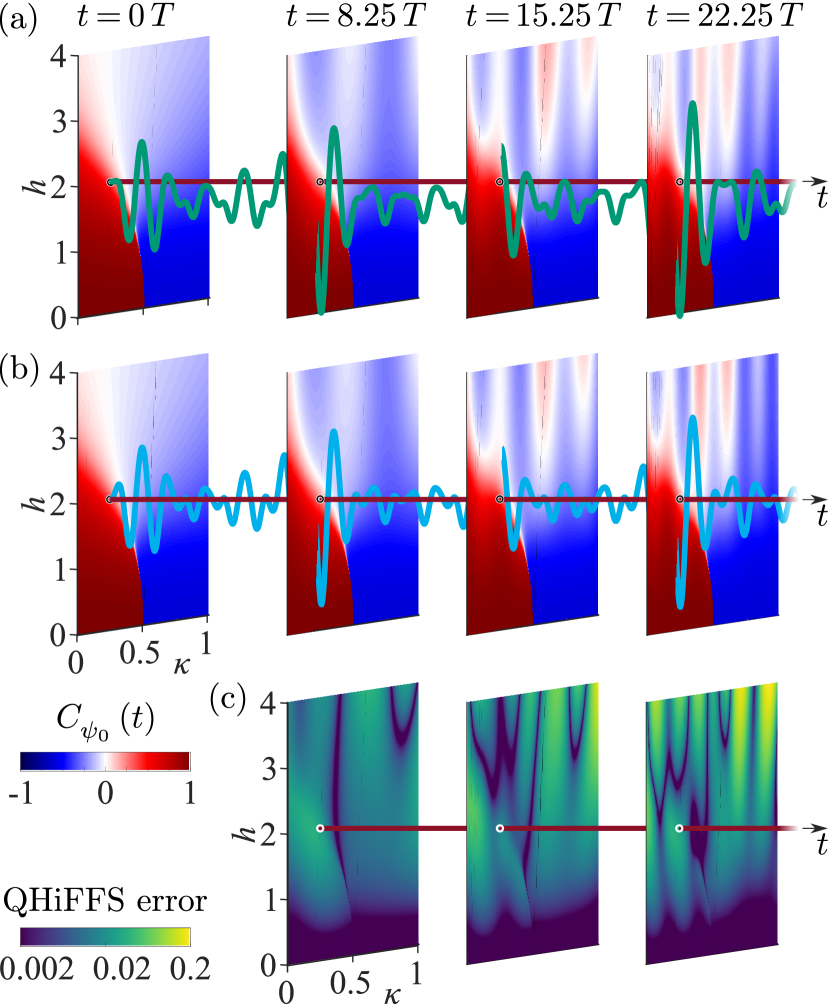
Figure 2: Numerical simulations of non-equilibrium dynamics of the transverse field BNNNI model. Two-dimensional slices of the next-nearest-neighbor correlation function, $C_{\psi_{0}}(t)$, as a function of $h$ and $\kappa$ for different simulation times $t$ computed exactly (a) and computed via $1^{\rm st}$ order QHiFFS (b). Here $J=1$ and $\omega=30$. The green/blue curves plot the exact/QHiFFS correlation function $C_{\psi_{0}}(t)$ as a function of time for the parameters $h=2$ and $\kappa=0.25$ also used in our hardware implementation (Fig. 3). In (c) we plot in logscale the error in the correlation function computed via QHiFFS - that is, the difference between the slices shown in (a) and (b). Videos corresponding to this figure can be found in the supplemental material.

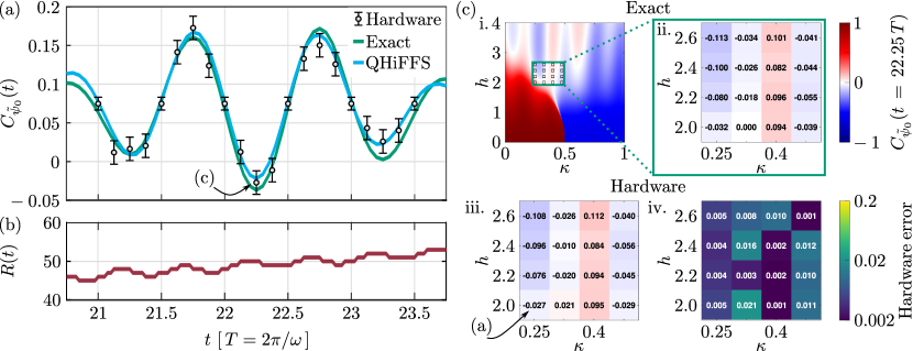
Figure 3: Hardware results: (a) Here we plot $C_{\tilde{\psi_{0}}}(t)$, Eq. (9), the next-nearest-neighbor correlation function, for our short depth approximation of the ground (initial) state $\ket{\tilde{\psi_{0}}}$ averaged over all qubit sites $k,l$. The green line gives the exact correlation function value and the blue line is the correlation function as computed using the first order QHiFFS ansatz, which is implementable on quantum hardware by a shallow circuit (shown in Appendix A). The black data points are hardware results obtained from a 20-qubit Quantinuum H1-1 quantum computer. Their $2\sigma$-error bars quantify uncertainty of the results due to finite shot number. (b) The red line compares the gate overhead required by Trotterization for the same (noise-free) algorithmic fidelity. That is, we plot $R(t)=N_{\rm Trotter}(t)/N_{\rm QHiFFS}(t)$ where $N_{\rm Trotter}(t)$ ($N_{\rm QHiFFS}(t)$) is the number of 2-qubit gates to simulate to time $t$ with a second order Trotterization (the first order QHiFFS). To make $R(t)$ a fair comparison metric, the time step for the Trotterization is set to ensure the algorithmic error is the same for both methods. (c) Here we plot the $C_{\psi}(t)$ dependence on the parameters $h$ and $\kappa$ for a zoomed in region of the total parameter space (i.) at time $t=22.25\,T$. (ii.) and (iii.) plot the exact correlation function values and those computed on quantum hardware respectively, with the error between them shown in (iv.).

The transverse field BNNNI model is an example of an Ising model with next-nearest neighbor axial interactions Elliott (1961); Bak and von Boehm (1980); Selke (1988); Alba and Fagotti (2017). Interest in such models is largely motivated by the following key facts: Firstly, the zero-temperature critical behavior of the quantum spin Ising system in $D$-dimensions is connected to the classical critical behavior of the corresponding $(D+1)$-dimensional classical system. Secondly, the results of such systems can provide insight into the general role of quantum fluctuations in quantum magnetism and also have direct relevance to experiments on numerous frustrated quantum magnets Nekrashevich et al. (2022) including CeSb Bak and von Boehm (1980), ${\rm Ag_{3}Mg}$ Selke (1988), ${\rm Sn_{2}P_{2}S_{6}}$ Liubachko et al. (2020), ${\rm BaHo_{2}O_{4}}$ Prévost et al. (2018), ${\rm SrDy_{2}O_{4}}$ Gauthier et al. (2017). While most work has focused on studying non-driven models, the non-equilibrium quantum dynamics of one-dimensional models has also been explored in a quench protocol Alba and Fagotti (2017); Kennes et al. (2018).

Here we consider the two-dimensional Floquet driven transverse field BNNNI model Hornreich et al. (1979) defined on a square lattice with the Hamiltonian

$$\hat{H}(t)=J \left(-\sum_{\langle i,j\rangle}\hat{Z}_{i}\hat{Z}_{j}+\kappa\sum_{\langle\langle i,j\rangle\rangle}\hat{Z}_{i}\hat{Z}_{j}\right)$$ (8)

$$-h\cos(\omega t)\sum_{i}\hat{X}_{i}\,.$$

Here $\hat{Z},\hat{X}$ are Pauli operators, $\sum_{\langle i,j\rangle}$ denotes a sum over the nearest neighbors, and $\sum_{\langle\langle i,j\rangle\rangle}$ is a sum over axial next-nearest neighbors as shown in Fig. 1(b). For simplicity, below we consider only the case of $J,\kappa>0$, for which the model is a paradigmatic example of frustrated magnetism.

Classical simulations of two-dimensional frustrated magnets are very challenging. Even their equilibrium properties are subject to long-standing controversy Savary and Balents (2016). In general, classically simulating their non-equilibrium properties is even more challenging, which has stimulated widespread interest in their quantum simulation Eisert et al. (2015). These challenges also limit our understanding of physics of the transverse field BNNNI model. Its static phase diagram is well-established for special cases. The zero-field ($h=0$) system exhibits a phase transition from a ferromagnetic phase to an antiphase at $\kappa_{c}=\frac{1}{2}$ Hornreich et al. (1979). In the ferromagnetic phase, all spins point in the same direction, while in the antiphase one finds periodic sequences of $2$ spins pointing in the same direction, followed by $2$ spins pointing in the opposite direction Hornreich et al. (1979). The presence of a transverse magnetic field, $h\hat{X}$, introduces additional quantum fluctuations. For $\kappa=0$, we recover the extensively studied transverse field quantum Ising model Pfeuty (1970); Pfeuty and Elliott (1971) with ferromagnetic order for $h<h_{c}\approx 3.04$ Blöte and Deng (2002). At $h_{c}$ the model undergoes a phase transition to a paramagnetic phase with all spins aligned in the $\hat{X}$ direction.

To probe dynamical properties and nonequilibrium phases of this model we study the next-nearest-neighbor correlation function averaged over all qubits on the lattice. That is, for an $n_{x}\times n_{y}$ lattice, we compute

$$C_{\psi}(t):=\frac{1}{n_{x}n_{y}}\sum_{l_{x}=0}^{n_{x}-1}\sum_{l_{y}=0}^{n_{y}-1}\Braket{\psi}{\hat{U}(t)^{\dagger}\hat{Z}_{l_{x},l_{y}}\hat{Z}_{l_{x},l_{y}+2}\hat{U}(t)}{\psi}$$ (9)

where $\ket{\psi}$ denotes an initial state of interest. To fit the lattice onto Quantinuum’s H1-1 quantum computer, in our hardware implementation, we consider a $4\times 5$ lattice with periodic boundary conditions. The correlator $C_{\psi_{0}}(t)>0$ indicates that directions of the next-nearest axial neighbor spins are aligned as in the ferromagnetic phase, while $C_{\psi_{0}}(t)<0$ indicates that they are anti-aligned (as in the antiphase). This quantity can serve to probe the field-induced phase change. In our case, we generally take $\ket{\psi}$ to be the ground state, denoted by $\ket{\psi_{0}}$ of $\hat{H}(t=0)$, setting $t_{0}=0$ in the following. The choice sets our simulations realistically connected with experimental situations. We stress that given the BNNNI model is translationally invariant, each term in the sum in Eq. (9) is identical and so $C_{\psi_{0}}(t)$ is equivalent to each of the individual qubit pair correlation functions. However, computing the average in Eq. (9) allows one to mitigate the effect of shot noise.

III.1 Numerical Simulations

We performed numerical simulations to study how well the QHiFFS algorithm captures short range correlation functions of the periodically driven BNNNI model. Figure 2(a) shows the next-nearest-neighbour correlation function, $C_{\psi_{0}}(t)$, as a function of $h$ and $\kappa$ for different simulation times. We chose $\omega=30$, which ensures the applicability of the kick approximation for all considered parameter values of the model. Regions of ferromagnetic and antiferromagnetic correlation are indicated in red and blue respectively. We see that periodic driving further enriches the physics of the BNNNI model. In particular, when the BNNNI system is driven out of equilibrium by a high-frequency high-strength transverse field, at long times a noticeable ferromagnetic instability can be induced out of an otherwise antiphase near the $\kappa=\frac{1}{2}$ quantum critical fan. This suggests that driven quantum systems are an exciting research area for generating and manipulating quantum phases.

Importantly, these complex changes are well-captured by the QHiFFS algorithm. This is shown in Fig. 2(b) where we plot the correlation function, $C_{\psi_{0}}(t)$, as computed using the QHiFFS algorithm. Indeed, as shown in Fig. 2(c), the errors in the correlation function (that is, the difference between the exact correlation function and the one computed via QHiFFS) are small. Specifically, the correlation function error on average (over the different $h$ and $\kappa$ values) is 0.0121 at $t=8.25\,T$, 0.0175 at $t=15.25\,T$ and 0.0216 at $t=22.25\,T$.

III.2 Hardware Implementation

To demonstrate the suitability of the QHiFFS algorithm for real quantum hardware we used all 20 qubits of Quantinuum’s H1-1 trapped ion platform to simulate the $4\times 5$ BNNNI model with periodic boundary conditions (see Fig. 1). This was enabled by the all-to-all connectivity of the platform – on superconducting circuit devices (as compared to the trapped ion device that we used here), periodic boundary conditions on two-dimensional lattice models are typically hard to implement due to the restriction to nearest-neighbor gates.

Due to a finite sampling budget of approximately 30,000 shots, we needed to restrict ourselves to specific model parameters. We decided to implement two studies - the first a simulation of the correlation function as a function of time, the second a slice of the correlation function at a fixed time plotted versus the model parameters. Without loss of generality, we took $J=1$. For our plot of the correlation function as a function of time, we then chose $h=2$, $\kappa=0.25$, and $\omega=30$ for which our numerical results indicate strong effects of periodic driving. For our study of model parameter dependence, we took $t=22.25\,T$ and focused on the region $0.25\leqslant\kappa\leqslant 0.475$ and $2.0\leqslant h\leqslant 2.6$. The chosen parameters ensured that all model parameters are of a similar order of magnitude resulting in strong frustration and quantum fluctuations.

The first order QHiFFS ansatz yielded a constant depth circuit for Floquet time evolution, as both $\exp(-it\hat{H}_{\mathrm{eff}})$ and $\exp(\pm i\hat{K}(t))$ were exactly implementable. Indeed, in the case of Quantinuum’s H1-1 trapped ion device, with native single qubit rotations and two-qubit gates $\exp(-i\frac{\theta}{2}\hat{Z}\hat{Z})$, the simulation was implemented exactly with a fixed circuit using the native gate set. This meant that the QHiFFS circuit, for any simulation time, had the same depth as a single standard low-order Trotter-Suzuki step. Thus, the final simulation time $t$ affected the error from the high-frequency approximation, but not the error from hardware imperfections.

Initial state preparation for a physically motivated quantum simulation is a non-trivial task, in general. In our case, preparing the ground states exactly would require deep circuits but using classical compilation techniques we found an approximation of the ground state that still captured the same underlying physics and required a much shorter depth circuit to prepare. Our final circuits used $40$ $2$-qubit gates to prepare an approximation of the ground state for different $h$ and $\kappa$ with an average overlap of $0.964$ relative to the true ground state. The complete quantum circuit for the full simulation consisted of $110$ $2$-qubit gates and $120$ single qubit gates (see Appendix A) for all non-half-integer time steps. At half-integer time steps the circuit implementing the time evolution compiled to the identity and so the circuit consisted of only the 40 gates required for state preparation.

In Fig. 3(a) we plot as a function of time: the correlation function obtained from our quantum hardware implementation (black data points), the exact value of the correlation function (green line) and the value predicted from classical simulations of the QHiFFS algorithm (blue line). Furthermore, for the hardware results we provide error bars quantifying their uncertainty due to a finite shot number as two standard deviations of the sample mean. Fig. 3(b) shows the ratio of the number of 2-qubit gates that would have been required for a Trotter simulation as compared to a QHiFFS simulation for the same average simulation fidelity. This varied from 45-fold (at short times) to 53-fold (at long times) and thus the Trotter simulation was not feasible to be implemented on quantum hardware.

In Fig. 3(c) we plot the zoomed in $C_{\psi}(t)$ dependence on the parameters at time $t=22.25\,T$ computed exactly and as computed on quantum hardware. The hardware error is less than 0.021 for all data points. Our implementation successfully captures the noticeable ferromagnetic instability induced out of the antiphase at the $\kappa=\frac{1}{2}$ quantum critical fan. This suggests that QHiFFS could open up new avenues to study novel driven quantum phases and criticality in strongly correlated electron systems. This could become particularly relevant experimentally when material systems with interesting high energy scales are subject to an electromagnetic field (e.g., light, high-harmonic generation).

The expected values of the correlation function are largely within our shot-noise based error bars, implying that our simulation (despite the considerable circuit depth and qubit number) is predominantly shot noise limited. Indeed, the simulation is also limited by the size of the available hardware - we chose to study a 20 qubit simulation not because this was the largest QHiFFS could handle, but rather because the Quantinuum H1-1 system was the largest all-to-all device to which we had access.

III.3 Error Analysis

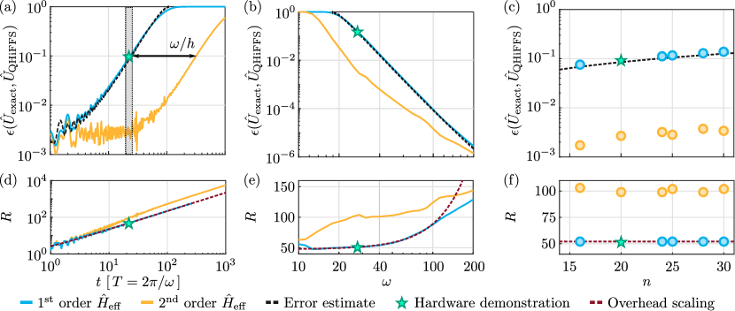
Figure 4: Error analysis. Here we plot the average fidelity as a function of (a) simulation time $t$, (b) frequency $\omega$ and (c) system size $n$. Unless varied, the parameters equal those of our hardware implementation in Fig. 3; namely $J\,=\,1$, $\kappa\,=\,0.25$, $h\,=\,2$, $\omega\,=\,30$ and $t\,=\,22.75\,T$. Overall, we find an excellent agreement between our analytical error estimate (black) and the exact numerical calculations (cyan). (Note, we plot here the full 1st-order expression for the error given in Eq. (12) in Appendix B). The yellow line indicates the exact error when $\hat{H}_{\rm eff}$ is expanded to second order in $\omega$ and the kick operator is expanded to first order in $\omega$. (d), (e) and (f) show the numerically calculated overhead of standard Trotterization $R$ in terms of simulation time $t$, frequency $\omega$ and system size $n$. For first order QHiFFS (cyan) we observe linear, quadratic (since $t$ is chosen in units of $T=\frac{2\pi}{\omega}$) and constant scalings with $t$, $\omega$ and $n$ respectively (shown in red) as predicted by Eq. (13).

To place the algorithm on solid conceptual foundations, as well as better understand the results of our numerical simulations and hardware implementations, we have conducted an analysis of QHiFFS algorithmic errors. To quantitatively judge the quality of a given Floquet simulation, we consider the average simulation infidelity over the uniform distribution of input states

$$\epsilon(\hat{U}_{1},\hat{U}_{2}):=1-\mathbb{E}\left.\left[\left|\Braket{\psi}{\hat{U}_{1}^{\dagger}\hat{U}_{2}}{\psi}\right|^{2}\right]\right|_{\ket{\psi}\sim\mathrm{Haar}_{n}}\,.$$ (10)

Here we provide a summary of our error analysis for the transversely driven BNNNI model. In Appendix B, we frame our error analysis more generally.

We start by analysing the scaling of errors for the standard Trotterisation approach. As shown in detail in Appendix C, there are three sources of error in this case, one coming from the discretization of the time-ordered integral, one coming from the non-commutativity of the Hamiltonian at different times and another (the standard time-independent Trotter error) coming from the non-commutativity of terms in the Hamiltonian at a fixed time. The dominant contribution in the high-frequency regime comes from discretization, while the errors from non-commutativity are comparably small. We find that the average infidelity for the transverse BNNNI model scales as

$$\epsilon(\hat{U}_{\textrm{exact}}(t),\hat{U}_{\textrm{Trotter}}(t))=\mathcal{O}\left(\frac{nh^{2}t^{4}\omega^{2}}{8m^{2}}\right).$$ (11)

where $m$ is the number of Trotter steps and $n$ is the system size. Thus, in contrast to standard time-independent Trotterization, the error here is independent of $\hat{H}_{0}$ and scales as $t^{4}$ rather than $t^{2}$.

In comparison, we find that the long time error for the transversely driven BNNNI model when simulated by QHiFFS, scales as

$$\epsilon(\hat{U}_{\textrm{exact}}(t),\hat{U}_{\textrm{QHiFFS}}(t))\approx\frac{281}{32}\frac{n\cdot h^{4}\cdot(1+\kappa^{2})\cdot J^{2}\cdot t^{2}}{\omega^{4}}\,.$$ (12)

The dominant contribution here is from the high-frequency truncation of the effective Hamiltonian. At short times, the truncation of the Kick approximation also contributes a significant oscillatory error to the averaged infidelity. However, the relative significance of this effect is washed out at longer times due to the contribution from the effective Hamiltonian which grows quadratically in time (compare Appendix B).

To support our analysis, we numerically computed the exact errors for the transversely driven BNNNI model. Specifically, in Fig. 4 we plot these errors, and our corresponding error estimates for the parameter regime we simulated on quantum hardware. Namely, a $4\times 5$ two-dimensional transversely-driven BNNNI model with $J=1$, $\kappa=0.25$, $h=2$, $\omega=30$ (in (a)) and $t=22.75T$ (in (b)). Overall, we find an excellent, nearly indistinguishable, agreement with our analysis.

Our error analysis further allows us to estimate how the circuit depth of a standard Trotterization needs to scale compared to QHiFFS to achieve the same fidelity. Let $R$ be the ratio of the number of two qubit gates used by Trotterization compared to the number of two qubit gates used by QHiFFS. For the driven BNNNI model presented here $R=m$, the number of Trotter steps used by the Trotterization since the $1^{\rm st.}$ order QHiFFS requires the same number of two qubit gates as one ($1^{\rm st.}$ or $2^{\rm nd.}$ order) Trotter step. Specifically, using Eq. (11) and Eq. (12) we find that for the two-dimensional driven BNNNI model, $R$ scales as

$$R=\mathcal{O}\left(\frac{t\omega^{3}}{Jh\sqrt{1+\kappa^{2}}}\right)\,.$$ (13)

This scaling well-reproduces that computed numerically. Namely, the Trotter overhead grows linearly in time, as shown in Fig. 3(b) and Fig. 4(d), and cubically in $\omega$, as shown in Fig. 4(e). We stress that this observation is independent of system size, $n$, as shown in Fig. 4(f).

The advantage of the QHiFFS ansatz can be further boosted by truncation at higher orders in $k$, (i.e. $(1/\omega)^{k}$). If we truncate at order $k$, the ratio of circuit depths becomes

$$R=\mathcal{O}\left(\frac{t\omega^{2}}{J\sqrt{1+\kappa^{2}}}\left(\frac{\omega}{h}\right)^{k}\right)\,.$$ (14)

Such higher order expansions open up the simulation of longer times and larger system sizes without increasing the algorithmic approximation infidelity, giving a significant advantage to the QHiFFS approach.

IV Discussion

Here we have proposed the QHiFFS algorithm for simulating periodically driven systems on digital quantum computers. Central to the algorithm is the use of a kick operator to transform the problem into a frame of reference where the dynamics of the system is governed by a time-independent effective Hamiltonian. Thus, this method avoids the costly discretization of the time-ordered integral required by standard Trotterization and allows one to re-use previous time-independent Hamiltonian simulation methods Verstraete et al. (2009); Berry et al. (2015); Low and Chuang (2019); Cirstoiu et al. (2020); Gibbs et al. (2021); Mansuroglu et al. (2021); Gibbs et al. (2022). In parallel, QHiFFS does not require any form of variational optimization of the sort required by many other near-term simulation methods Cirstoiu et al. (2020); Gibbs et al. (2021, 2022); Mansuroglu et al. (2021); Endo et al. (2020); Yao et al. (2021); Kökcü et al. (2021); Gu et al. (2021a).

In special cases, namely those where the non-interacting Hamiltonian is diagonal and the driving term involves only a single local driving term, a fixed depth circuit can be used to simulate arbitrary times with an algorithmic error that grows quadratically in time. Thus, in this limit, the QHiFFS algorithm provides a new method for approximate fast-forwarding quantum simulations Cirstoiu et al. (2020); Gibbs et al. (2021, 2022); Kökcü et al. (2021); Gu et al. (2021b) that is highly suitable to near-term hardware. We stress that while the simulation in such cases is particularly simple, and thus also simpler to simulate classically, we still expect QHiFFS to be a useful stepping stone towards quantum advantage. This is because even the fixed depth circuits enabled by the kick approximation could be challenging to simulate classically. In general, apart from special cases like Clifford circuits or one-dimensional low entangled states Fannes et al. (1992); Verstraete et al. (2008), the classical cost of simulating quantum circuits grows exponentially with circuit depth Liu et al. (2021). Therefore, one may expect that sufficiently deep and entangling fixed-depth QHiFFS circuits will be challenging to simulate classically in higher spatial dimensions. Given that these gate sequences are good approximations of the dynamics of quantum many-body systems that are forced out of equilibrium by a high frequency drive, such strong entanglement generation is a natural expectation.

Furthermore, even in the case where QHiFFS is classically simulable for some input states, it could still be used to implement classically intractable simulations for non-classically simulable initial states. Such states could plausibly be prepared via analogue simulation strategies. This could provide one of the earliest avenues for physically interesting non-classically simulable implementations of QHiFFS on near-term hardware.

However, QHiFFS is also much more broadly applicable and we expect the algorithm to find use in the fault-tolerant era as well as the near-term. In the latter case, one could use higher order expansions of the effective Hamiltonian and kick operators to achieve a higher accuracy, and implement the more complex resulting effective Hamiltonian using well-established fault-tolerant simulation methods Berry et al. (2015); Low and Chuang (2019).

To benchmark QHiFFS we performed a 20-qubit simulation of the periodically driven two-dimensional BNNNI model on Quantinuum’s 20-qubit H1-1 trapped ion platform. As shown in Fig. 3, the correlation function values computed on the quantum computer capture the true predicted values up to the precision allowed by shot noise ($2\sigma=1.49\cdot 10^{-2}$). In contrast, standard Trotterization (specifically a 2^nd order Trotterization with the same algorithmic error as a 1^st order QHiFFS) would have required approximately 50 times as many two-qubit gates, making the method completely unfeasible on current hardware due to gate errors and decoherence.

Our error scaling analysis demonstrates that QHiFFS outperforms standard Trotterization for high driving frequencies, $\omega$. Specifically, at long simulation times, $t$, we see a linear advantage in $t$ and at least cubic improvements in $\omega$ compared to standard Trottterization. In parallel, the algorithmic errors of QHiFFS scale linearly in system size, $n$, for local models, and at worst quadratically. These favourable scalings again point towards QHiFFS’s suitability for larger scale implementations.

Future interesting applications of QHiFFS on quantum hardware could include the simulation of strongly correlated systems in the presence of linearly or circularly polarized electromagnetic field for the study of the emergence of unconventional superconductivity Kumar and Lin (2021), quantum spin liquids Claassen et al. (2017), and Kondo coherence collapse Zhu et al. (2021). Similarly, one could study even more complicated, approximately fast-forwardable Ising models, either by adding longer range interactions or by studying three spatial dimensions. We believe the latter would be viable with current gate fidelities, e.g. on Quantinuum’s trapped ion device, but (for a non-trivial simulation) would require more qubits.

one´

Supplementary Material for
“Large-scale simulations of Floquet physics on near-term quantum computers”

Appendix A Hardware quantum circuit

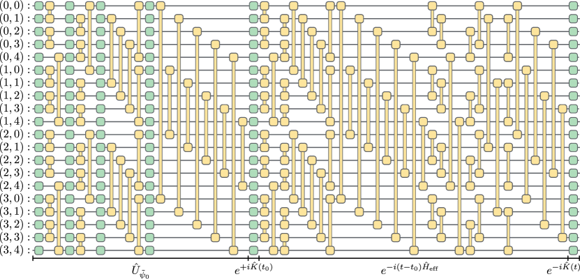
Figure 5: Quantinuum hardware circuit: One-qubit gates are colored in green and two-qubit gates are depicted in yellow. The first 4 two-qubit layers (40 gates) are used for approximate preparation of the BNNNI model ground-state $\ket{\psi_{0}}$ (average overlap $\approx 96.4$ %). The remaining 7 two-qubit layers (70 gates) are used to implement $\exp(-i(t-t_{0})\hat{H}_{\rm eff})\approx\exp(-i(t-t_{0})\hat{H}_{0})$. Both $\hat{K}(t)$ and $\hat{H}_{0}$ can be implemented exactly up to $\mathcal{O}\left(\frac{1}{\omega^{2}}\right)$, which allows for constant depth approximate fast-forwarding.

Appendix B QHiFFS Error Analysis

B.1 Derivation of kick operator and effective Hamiltonian

In this subsection we provide a detailed derivation of the effective Hamiltonian and kick operator for pedagogical purposes. This derivation was originally performed in Ref. Goldman and Dalibard (2014).

We start with a periodic, time-dependent Hamiltonian,

$$\hat{H}(t)=\hat{H}_{0}+\hat{V}(t),\qquad\hat{V}(t)=\hat{V}(t+T).$$ (15)

Our aim is to transform to a basis in which the time evolution is generated by an effective, time-independent Hamiltonian, $\hat{H}_{\rm eff}$,

$$i\partial_{t}\ket{\psi}=\hat{H}(t)\ket{\psi}\implies i\partial_{t}\ket{\phi}=\hat{H}_{\rm eff}\ket{\phi(t)}\qquad\textrm{for }\ket{\phi(t)}=e^{i\hat{K}(t)}\ket{\psi}\;.$$ (16)

The so-called kick operator $\hat{K}$ generates the basis change. Inserting the definition of $\ket{\phi}$ into the Schrödinger equation (Eq. (16)) gives a defining relation for the effective Hamiltonian

$$\hat{H}_{\rm eff}=e^{i\hat{K}(t)}\hat{H}(t)e^{-i\hat{K}(t)}+i\left(\frac{\partial e^{i\hat{K}(t)}}{\partial t}\right)e^{-i\hat{K}(t)}.$$ (17)

While Eq. (17) is hard to solve in general, consistent perturbative expansions of the kick operator, $\hat{K}(t)$, and effective Hamiltonian, $\hat{H}_{\rm eff}$, can be found in the high frequency regime. To do this, we expand in polynomial orders of the period, $\frac{T}{2\pi}=\frac{1}{\omega}$,

$$\hat{H}_{\rm eff}=\sum_{k=0}^{\infty}\frac{\hat{H}_{\rm eff}^{(k)}}{\omega^{k}}\;,\qquad\qquad\hat{K}(t)=\sum_{k=1}^{\infty}\frac{\hat{K}^{(k)}(t)}{\omega^{k}}\;.$$ (18)

Note that the kick operator is periodic with the same period, $T$, as the potential, $V(t)$, which can be seen from Eq. (17). We assume that the kick operator does not admit a constant 0^th order as it can be absorbed in $H_{0}$ without loss of generality. The first term on the right hand side of Eq. (17) can be expanded using the Hadamard lemma, i.e. we have

$$e^{i\hat{K}(t)}\hat{H}(t)e^{-i\hat{K}(t)} =\sum_{q=0}^{\infty}\frac{i^{q}}{q!}\left[\hat{K}(t)_{(q)},\hat{H}(t)\right]\;,$$ (19)

where we denote $q$-fold nested commutators by $\left[\hat{K}(t)_{(q)},\hat{H}(t)\right]=\left[\hat{K}(t),\left[\hat{K}(t)_{(q-1)},\hat{H}(t)\right]\right]$. The second term can then be expanded using the well-known identity $\frac{\partial}{\partial x}e^{\hat{A}(x)}=\int_{0}^{1}e^{y\hat{A}(x)}\left(\frac{\partial}{\partial x}\hat{A}(x)\right)e^{(1-y)\hat{A}(x)}dy$ and the Hadamard lemma, to give

$$i\left(\frac{\partial e^{i\hat{K}(t)}}{\partial t}\right)e^{-i\hat{K}(t)} =-\int_{0}^{1}e^{ix\hat{K}(t)}\left(\frac{\partial}{\partial t}\hat{K}(t)\right)e^{-ix\hat{K}(t)}dx=-\sum_{q=0}^{\infty}\frac{i^{q}}{(q+1)!}\left[\hat{K}_{(q)},\frac{\partial\hat{K}(t)}{\partial t}\right]\;.$$ (20)

Finally, we use a Fourier decomposition of the potential $\hat{V}(t)=\sum_{j=1}^{\infty}\hat{V}^{(j)}e^{ij\omega t}+\hat{V}^{(-j)}e^{-ij\omega t}$ to show its frequency dependence. Note that hermiticity of $\hat{V}(t)$ implies $\hat{V}^{(j)^{\dagger}}=\hat{V}^{(-j)}$. An order-by-order solution for $\hat{K}(t)$ and $\hat{H}_{\rm eff}$ can then be systematically achieved. For the $k^{th}$ order, the steps are thus,

1. Write down $k^{th}$ order of Eq. (17).

2. Plug in all orders up to $k-1$ for $\hat{H}_{\rm eff}$ and $k$ for $\hat{K}(t)$.

3. Define $\hat{K}^{(k+1)}(t)$ such that the right hand side of Eq. (17) is time independent.

4. Read off $\hat{H}_{\rm eff}^{(k)}$.

We demonstrate the method to find $\hat{K}(t)$ and $\hat{H}_{\rm eff}$ up to second order. The terms contributing to $0^{th}$ order in Eq. (17) are

$$\hat{H}_{\rm eff}^{(0)}=\hat{H}(t)-\frac{1}{\omega}\frac{\partial\hat{K}^{(1)}(t)}{\partial t}=\hat{H}_{0}+\sum_{j=1}^{\infty}\left(\hat{V}^{(j)}e^{ij\omega t}+\hat{V}^{(-j)}e^{-ij\omega t}\right)-\frac{1}{\omega}\frac{\partial\hat{K}^{(1)}(t)}{\partial t}\;.$$ (21)

Although $K^{(1)}$ comes with a first order factor $\frac{1}{\omega}$, the term involving the time derivative $\frac{\partial}{\partial t}K^{(1)}=\mathcal{O}(\omega)$ is of $0^{\rm th}$ order. This is because of the periodicity of $K(t)$ and can be straight-forwardly shown using the fact that the lowest frequency in its Fourier transform has to be $\omega$. To eliminate the time-dependence in Eq. (21), we define

$$\hat{K}^{(1)}(t)=-i\sum_{j=1}^{\infty}\frac{1}{j}\left(\hat{V}^{(j)}e^{ij\omega t}-\hat{V}^{(-j)}e^{-ij\omega t}\right)\;,$$ (22)

which leaves us with $\hat{H}_{\rm eff}^{(0)}=\hat{H}_{0}$. Next, to first order

$$\frac{1}{\omega}\hat{H}_{\rm eff}^{(1)} =\frac{i}{\omega}\left[\hat{K}^{(1)},\hat{H}(t)\right]-\frac{i}{2\omega^{2}}\left[\hat{K}^{(1)},\frac{\partial\hat{K}^{(1)}(t)}{\partial t}\right]-\frac{1}{\omega^{2}}\frac{\partial\hat{K}^{(2)}(t)}{\partial t}$$ (23)

$$\iff\hat{H}_{\rm eff}^{(1)} =\sum_{j=1}^{\infty}\frac{1}{j}\left(\left[\hat{V}^{(j)},\hat{H}_{0}\right]e^{ij\omega t}+H.c.\right)+\frac{1}{2}\sum_{j,k=1}^{\infty}\frac{1}{j}\left(\left[\hat{V}^{(j)},\hat{V}^{(k)}\right]e^{i(j+k)\omega t}+H.c.\right)$$

$$+\frac{1}{2}\sum_{j,k=1}^{\infty}\frac{1}{j}\left(\left[\hat{V}^{(j)},\hat{V}^{(-k)}\right]e^{i(j-k)\omega t}+H.c.\right)-\frac{1}{\omega}\frac{\partial\hat{K}^{(2)}(t)}{\partial t}\;.$$ (24)

Again, we identify the time-dependent terms and integrate them to fix

$$\hat{K}^{(2)}(t)= -i\sum_{j=1}^{\infty}\frac{1}{j^{2}}\left(\left[\hat{V}^{(j)},\hat{H}_{0}\right]e^{ij\omega t}-H.c.\right)-\frac{i}{2}\sum_{j,k=1}^{\infty}\frac{1}{j(j+k)}\left(\left[\hat{V}^{(j)},\hat{V}^{(k)}\right]e^{i(j+k)\omega t}-H.c.\right)$$

$$-\frac{i}{2}\sum_{j\neq k=1}^{\infty}\frac{1}{j(j-k)}\left(\left[\hat{V}^{(j)},\hat{V}^{(-k)}\right]e^{i(j-k)\omega t}-H.c.\right).$$ (25)

and read off $\hat{H}_{\rm eff}^{(1)}=\sum_{j=1}^{\infty}\frac{1}{j}\left[\hat{V}^{(j)},\hat{V}^{(-j)}\right]$. Finally, we calculate $\hat{H}_{\rm eff}$ to second order,

$$\frac{1}{\omega^{2}}\hat{H}_{\rm eff}^{(2)}= \frac{i}{\omega^{2}}\left[\hat{K}^{(2)},\hat{H}(t)\right]-\frac{1}{2\omega^{2}}\left[\hat{K}^{(1)},\left[\hat{K}^{(1)},\hat{H}(t)\right]\right]+\frac{1}{6\omega^{3}}\left[\hat{K}^{(1)},\left[\hat{K}^{(1)},\frac{\partial\hat{K}^{(1)}(t)}{\partial t}\right]\right]$$

$$-\frac{i}{2\omega^{3}}\left[\hat{K}^{(1)},\frac{\partial\hat{K}^{(2)}(t)}{\partial t}\right]-\frac{i}{2\omega^{3}}\left[\hat{K}^{(2)},\frac{\partial\hat{K}^{(1)}(t)}{\partial t}\right]-\frac{1}{\omega^{3}}\frac{\partial\hat{K}^{(3)}(t)}{\partial t}\;.$$ (26)

We can simplify this expression by first plugging in $\frac{\partial\hat{K}^{(1)}}{\partial t}=\omega\hat{V}(t)$.

$$\hat{H}_{\rm eff}^{(2)}= i\left[\hat{K}^{(2)},\hat{H}_{0}\right]+\frac{i}{2}\left[\hat{K}^{(2)},\hat{V}(t)\right]-\frac{1}{2}\left[\hat{K}^{(1)},\left[\hat{K}^{(1)},\hat{H}_{0}\right]\right]-\frac{1}{3}\left[\hat{K}^{(1)},\left[\hat{K}^{(1)},\hat{V}(t)\right]\right]$$

$$-\frac{i}{2\omega}\left[\hat{K}^{(1)},\frac{\partial\hat{K}^{(2)}(t)}{\partial t}\right]-\frac{1}{\omega}\frac{\partial\hat{K}^{(3)}(t)}{\partial t}$$ (27)

We are more interested in $\hat{H}_{\rm eff}^{(2)}$ than in $\hat{K}^{(3)}$, so we drop all time-dependent terms to find,

$$\hat{H}_{\rm eff}^{(2)}= \frac{1}{2}\sum_{j=1}^{\infty}\frac{1}{j^{2}}\left(\left[\left[\hat{V}^{(j)},\hat{H}_{0}\right],\hat{V}^{(-j)}\right]+H.c.\right)+\frac{1}{4}\sum_{j,k=1}^{\infty}\frac{1}{j(j+k)}\left(\left[\left[\hat{V}^{(j)},\hat{V}^{(k)}\right],\hat{V}^{(-j-k)}\right]+H.c.\right)$$

$$+\frac{1}{4}\sum_{j\neq k=1}^{\infty}\frac{1}{j(j-k)}\left(\left[\left[\hat{V}^{(j)},\hat{V}^{(-k)}\right],\hat{V}^{(k-j)}\right]+H.c.\right)-\frac{1}{2}\sum_{j=1}^{\infty}\frac{1}{j^{2}}\left(\left[\hat{V}^{(j)},\left[\hat{V}^{(-j)},\hat{H}_{0}\right]\right]+H.c.\right)$$

$$+\frac{1}{3}\sum_{j,k=1}^{\infty}\frac{1}{jk}\left(\left[\hat{V}^{(j)},\left[\hat{V}^{(k)},\hat{V}^{(-j-k)}\right]\right]+H.c.\right)-\frac{1}{3}\sum_{j\neq k=1}^{\infty}\frac{1}{jk}\left(\left[\hat{V}^{(j)},\left[\hat{V}^{(-k)},\hat{V}^{(k-j)}\right]\right]+H.c.\right)$$

$$+\frac{1}{2}\sum_{j=1}^{\infty}\frac{1}{j^{2}}\left(\left[\hat{V}^{(-j)},\left[\hat{V}^{(j)},\hat{H}_{0}\right]\right]+H.c.\right)+\frac{1}{4}\sum_{j,k=1}^{\infty}\frac{1}{j(j+k)}\left(\left[\hat{V}^{(-j-k)},\left[\hat{V}^{(j)},\hat{V}^{(k)}\right]\right]+H.c.\right)$$

$$+\frac{1}{4}\sum_{j\neq k=1}^{\infty}\frac{1}{j(j-k)}\left(\left[\hat{V}^{(k-j)},\left[\hat{V}^{(j)},\hat{V}^{(-k)}\right]\right]+H.c.\right)$$ (28)

$$= -\frac{1}{2}\sum_{j=1}^{\infty}\frac{1}{j^{2}}\left(\left[\hat{V}^{(j)},\left[\hat{V}^{(-j)},\hat{H}_{0}\right]\right]+H.c.\right)+\frac{1}{3}\sum_{j,k=1}^{\infty}\frac{1}{jk}\left(\left[\hat{V}^{(j)},\left[\hat{V}^{(k)},\hat{V}^{(-j-k)}\right]\right]+H.c.\right)$$

$$-\frac{1}{3}\sum_{j\neq k=1}^{\infty}\frac{1}{jk}\left(\left[\hat{V}^{(j)},\left[\hat{V}^{(-k)},\hat{V}^{(k-j)}\right]\right]+H.c.\right)\;,$$ (29)

which has contributions from all terms of Eq. (27) except $i\left[\hat{K}^{(2)},\hat{H}_{0}\right]$ and $-\frac{1}{\omega}\frac{\partial\hat{K}^{(3)}(t)}{\partial t}$, which do not include time-independent terms. Putting together all terms up to second order, we find,

$$\hat{H}_{\rm eff}=\hat{H}_{0} +\frac{1}{\omega}\sum_{j=1}^{\infty}\frac{1}{j}\left[\hat{V}^{(j)},\hat{V}^{(-j)}\right]-\frac{1}{2\omega^{2}}\sum_{j=1}^{\infty}\frac{1}{j^{2}}\left(\left[\hat{V}^{(j)},\left[\hat{V}^{(-j)},\hat{H}_{0}\right]\right]+H.c.\right)$$

$$+\frac{1}{3}\sum_{j,k=1}^{\infty}\frac{1}{jk}\left(\left[\hat{V}^{(j)},\left[\hat{V}^{(k)},\hat{V}^{(-j-k)}\right]\right]+H.c.\right)-\frac{1}{3}\sum_{j\neq k=1}^{\infty}\frac{1}{jk}\left(\left[\hat{V}^{(j)},\left[\hat{V}^{(-k)},\hat{V}^{(k-j)}\right]\right]+H.c.\right)+\mathcal{O}\left(\frac{1}{\omega^{3}}\right)\;,$$ (30)

$$\hat{K}(t)= -\frac{i}{\omega}\sum_{j=1}^{\infty}\frac{1}{j}\left(\hat{V}^{(j)}e^{ij\omega t}-\hat{V}^{(-j)}e^{-ij\omega t}\right)-\frac{i}{\omega^{2}}\sum_{j=1}^{\infty}\frac{1}{j^{2}}\left(\left[\hat{V}^{(j)},\hat{H}_{0}\right]e^{ij\omega t}-H.c.\right)$$

$$-\frac{i}{2\omega^{2}}\sum_{j,k=1}^{\infty}\frac{1}{j(j+k)}\left(\left[\hat{V}^{(j)},\hat{V}^{(k)}\right]e^{i(j+k)\omega t}-H.c.\right)$$

$$-\frac{i}{2\omega^{2}}\sum_{j\neq k=1}^{\infty}\frac{1}{j(j-k)}\left(\left[\hat{V}^{(j)},\hat{V}^{(-k)}\right]e^{i(j-k)\omega t}-H.c.\right)+\mathcal{O}\left(\frac{1}{\omega^{3}}\right)$$ (31)

It becomes apparent from the above derivation that all orders of $\hat{K}(t)$ and $\hat{H}_{\rm eff}$ consist of commutator terms. Also note that in this work, the Fourier components of the driving potential commute, which further simplifies the high frequency expansion.

B.2 Special cases

Property of $\hat{H}_{0}$	Property of $\hat{V}(t)$	Implications and implementation strategy	Form of $\hat{H}_{\rm eff}$ and $\hat{K}(t)$
$[\hat{H}_{0},\hat{V}(t)]=0\,\forall t$	Single frequency	Trivial case. Standard Trotterization and the kick operator ansatz coincide.	(36 - 37)
	Multiple frequencies	Different Fourier components $\hat{V}^{(j)}$ might not commute which creates effective dynamics.	(34 - 35)
$[\hat{H}_{0},\hat{V}(t)]\neq 0$	Single frequency	Corrections only from $[\hat{H}_{0},\hat{V}(t)]$. This allows us to re-use previous time-independent techniques and lift them to Floquet Hamiltonian simulation.	(32 - 33)
	Multiple frequencies	Most general case taking into account all effective dynamics.	(30 - 31)

Table 1: Comparison of special cases for the application to kick approximation

Table 1 lists different special cases that can simplify expressions for $\hat{H}_{\rm eff}$ and $\hat{K}(t)$. We discuss the four classes of periodic systems in the following. Starting with the expressions (30, 31) derived above, assume the periodic potential only admits a single frequency component $\hat{V}^{(1)}$ in its Fourier transformation $\hat{V}^{(-1)}$. Assuming $\left[\hat{V}^{(1)},\hat{V}^{(-1)}\right]=0$, we obtain,

$$\hat{H}_{\rm eff} =\hat{H}_{0}-\frac{1}{2\omega^{2}}\left(\left[\hat{V}^{(1)},\left[\hat{V}^{(-1)},\hat{H}_{0}\right]\right]+H.c.\right)+\mathcal{O}\left(\frac{1}{\omega^{3}}\right)\;,$$ (32)

$$\hat{K}(t) =-\frac{i}{\omega}\left(\hat{V}^{(1)}e^{i\omega t}-\hat{V}^{(-1)}e^{-i\omega t}\right)-\frac{i}{\omega^{2}}\left(\left[\hat{V}^{(1)},\hat{H}_{0}\right]e^{i\omega t}-H.c.\right)+\mathcal{O}\left(\frac{1}{\omega^{3}}\right).$$ (33)

Interestingly, the first order terms of $\hat{H}_{\rm eff}$ vanish. As long as the potential is 1-local, $\hat{H}_{\rm eff}$ will also not grow in locality, making it implementable on quantum hardware without further compilation. Another simplification arises if $[\hat{H}_{0},\hat{V}(t)]=0\,\forall t$ or equivalently $\left[\hat{H}_{0},\hat{V}^{(j)}\right]=\left[\hat{H}_{0},\hat{V}^{(j)}\right]=0\,\forall j$. If we admit arbitrary potentials, we obtain,

$$\hat{H}_{\rm eff} =\hat{H}_{0}+\frac{1}{\omega}\sum_{j=1}^{\infty}\frac{1}{j}\left[\hat{V}^{(j)},\hat{V}^{(-j)}\right]-\frac{1}{3\omega^{2}}\sum_{j,k=1}^{\infty}\frac{1}{j(j+k)}\left(\left[\hat{V}^{(j+k)},\left[\hat{V}^{(-j)},\hat{V}^{(-k)}\right]\right]+H.c.\right)$$

$$-\frac{1}{3\omega^{2}}\sum_{j\neq k=1}^{\infty}\frac{1}{j(j-k)}\left(\left[\hat{V}^{(j-k)},\left[\hat{V}^{(-j)},\hat{V}^{(k)}\right]\right]+H.c.\right)+\mathcal{O}\left(\frac{1}{\omega^{3}}\right)\;,$$ (34)

$$K(t) =-\frac{i}{\omega}\sum_{j=1}^{\infty}\frac{1}{j}\left(\hat{V}^{(j)}e^{ij\omega t}-\hat{V}^{(-j)}e^{-ij\omega t}\right)-\frac{i}{2\omega^{2}}\sum_{j,k=1}^{\infty}\frac{1}{j(j+k)}\left(\left[\hat{V}^{(j)},\hat{V}^{(k)}\right]e^{i(j+k)\omega t}-H.c.\right)$$

$$-\frac{i}{2\omega^{2}}\sum_{j\neq k=1}^{\infty}\frac{1}{j(j-k)}\left(\left[\hat{V}^{(j)},\hat{V}^{(-k)}\right]e^{i(j-k)\omega t}-H.c.\right)+\mathcal{O}\left(\frac{1}{\omega^{3}}\right)\;.$$ (35)

Here, $\hat{H}_{0}$ does not appear in higher order terms. This makes quantum simulation particularly simple, if the potential is 1-local since then $\hat{K}(t)$ and all corrections in $\hat{H}_{\rm eff}$ will be 1-local. For $p$-local $\hat{V}$, locality grows in general which introduces additional challenges for implementation. If both simplifications, $\left[\hat{H}_{0},\hat{V}(t)\right]=0$ and a single frequency driving with $\left[\hat{V}^{(j)},\hat{V}^{(-j)}\right]=0$, are given, the lowest order kick approximation becomes exact

$$\hat{H}_{\rm eff} =\hat{H}_{0}$$ (36)

$$\hat{K}(t) =-\frac{i}{\omega}\left(\hat{V}^{(1)}e^{i\omega t}-\hat{V}^{(-1)}e^{-i\omega t}\right).$$ (37)

Note that since $\hat{K}(t)$ just denotes an integration of $\hat{V}(t)$, we have reduced the kick approximation to a simple case of Trotterization.

In the third case of Table 1, namely $\left[\hat{H}_{0},\hat{V}(t)\right]\neq 0$ and a single frequency driving with $\left[\hat{V}^{(j)},\hat{V}^{(-j)}\right]=0$, a known implementation of the simulation under $\hat{H}_{0}$ comes in handy. Since the first order correction in $\hat{H}_{\rm eff}$ vanishes, simulating $\hat{H}_{0}$ alone already yields a good approximation to high frequency dynamics. In the simplest non-trivial case, $\hat{H}_{0}$ is diagonal as in the BNNNI model discussed in the main text. In that case, $\hat{H}_{0}$ can be simulated using a constant depth circuit. Similar cases of known implementations of $\hat{H}_{0}$ are 1D XY-models Verstraete et al. (2009), Bethe diagonalizable models Sopena et al. (2022), and translational invariant models Mansuroglu et al. (2021).

B.3 Leading error terms

Intimately related to the output fidelity is the Hilbert-Schmidt product of unitaries (cf. Eq. (10)), which we will focus on in the following error analysis. The error $\xi$ which we derive in the following appears in the Hilbert-Schmidt product as follows ${\rm Tr}\left(U_{1}^{\dagger}U_{2}\right)=d(1-\xi)$ with the Hilbert space dimension $d$. In general, we have

$$\epsilon(\hat{U}_{1},\hat{U}_{2})=1-\frac{1}{d^{2}}{\rm Tr}\left(\hat{U}_{1}^{\dagger}\hat{U}_{2}\right)^{2}=:1-(1-\xi)^{2}=2\xi+\mathcal{O}(\xi^{2}).$$ (38)

$\xi$ can thus be seen as an estimate of the infidelity of a Haar random state undergoing evolution by $\hat{U}_{1}$ and $\hat{U}_{2}$ up to a factor of 2. Using permutation invariance of the trace, the Hilbert-Schmidt product between a kick approximation of first order and exact evolution reads

$${\rm Tr}(\hat{U}_{\rm exact}^{\dagger}(t_{0},t)\hat{U}_{\rm QHiFFS}(t_{0},t))={\rm Tr}\left(e^{i\tilde{K}(t_{0})}e^{-i\hat{K}(t_{0})}e^{i(t-t_{0})\hat{H}_{\rm eff}}e^{i\hat{K}(t)}e^{-i\tilde{K}(t)}e^{-i(t-t_{0})\tilde{H}_{\rm eff}}\right),$$ (39)

where $\tilde{K}(t)$ denotes the truncated Kick operator and $\hat{K}(t)$ contains all orders (similar for $\hat{H}_{\rm eff}$). As the trace of a commutator is always zero, ${\rm Tr}\left(\left[\hat{A},\hat{B}\right]\right)=0$, we will omit terms that contribute with a vanishing commutator term in what follows. We want to expand Eq. (39) step-by-step in orders of $\frac{1}{\omega}$ starting with the exponentials of $\hat{K}(t)$ and $\tilde{K}(t)$. Using the Baker-Campbell-Hausdorff (BCH) lemma

$$e^{i\hat{K}(t)}e^{-i\tilde{K}(t)}= \mathds{1}+i\frac{1}{\omega^{2}}\hat{K}^{(2)}(t)-\frac{1}{2\omega^{4}}\left(\hat{K}^{(2)}(t)\right)^{2}+\mathcal{O}\left(\frac{1}{\omega^{5}}\right).$$ (40)

Since the kick operator, $\hat{K}(t)$, as well as the effective Hamiltonian, $\hat{H}_{\rm eff}$, have a leading order error quadratic in $\frac{1}{\omega}$, which is a pure commutator, we expect the leading error of Eq. (39) to be of fourth order (39) as only products of commutators survive in the trace. The remaining factor will then be a similar combination of the exponentials of the effective Hamiltonians. This can be calculated with the following identity that follows from the Hadamard-Lemma

$$e^{\hat{A}}e^{-\hat{A}+\hat{\chi}}-\mathds{1}=\int_{0}^{1}ds\,e^{s\hat{A}}\hat{\chi}\,e^{-s\hat{A}}+\mathcal{O}(\hat{\chi}^{2})=\sum_{q=0}^{\infty}\frac{1}{(q+1)!}\left[\hat{A}_{(q)},\hat{\chi}\right]+\mathcal{O}(\hat{\chi}^{2})\;,$$ (41)

as before we denoted $q$-fold nested commutators by $\left[\hat{A}_{(q)},\hat{\chi}\right]=\left[\hat{A},\left[\hat{A}_{(q-1)},\hat{\chi}\right]\right]$. Applied to the remaining factors of Eq. (39), we define the second order error term of the effective Hamiltonian $\hat{H}_{\rm eff}$ as

$$e^{i(t-t_{0})\hat{H}_{\rm eff}}e^{-i(t-t_{0})\tilde{H}_{\rm eff}} =\mathds{1}+\sum_{q=0}^{\infty}\frac{i^{q+1}(t-t_{0})^{q+1}}{(q+1)!}\frac{1}{\omega^{2}}\left[\hat{H}_{0(q)},\hat{H}_{\rm eff}^{(2)}\right]+\mathcal{O}\left(\frac{1}{\omega^{3}}\right)$$

$$=:\mathds{1}+\hat{\Delta}_{\rm eff}^{(2)}(t-t_{0})+\mathcal{O}\left(\frac{1}{\omega^{3}}\right),$$ (42)

where we used $\hat{A}:=\hat{H}_{\rm eff}$ and $\hat{\chi}=\hat{H}_{\rm eff}-\tilde{H}_{\rm eff}$. $\hat{\Delta}_{\rm eff}$ again consists of commutators only and will consist of a series of infinitely many non-vanishing terms, in general. Later, we will use the integral formula (41) to evaluate $\hat{\Delta}_{\rm eff}^{(2)}$ for the model under consideration. Taking all factors together and plugging back into Eq. (39), we obtain

$${\rm Tr}(\hat{U}_{\rm exact}^{\dagger}(t_{0},t)\hat{U}_{\rm QHiFFS}(t_{0},t))=d +\frac{1}{\omega^{4}}{\rm Tr}\Bigg{(}\frac{1}{2}\left(\hat{\Delta}_{\rm eff}^{(2)}(t-t_{0})\right)^{2}-i\hat{K}^{(2)}(t_{0})\hat{\Delta}_{\rm eff}^{(2)}(t-t_{0})-i\hat{K}^{(2)}(t)\hat{\Delta}_{\rm eff}^{(2)}(t_{0}-t)+$$

$$+\hat{K}^{(2)}(t_{0})e^{i(t-t_{0})\hat{H}_{0}}\hat{K}^{(2)}(t)e^{-i(t-t_{0})\hat{H}_{0}}-\frac{1}{2}\left(\hat{K}^{(2)}(t_{0})\right)^{2}-\frac{1}{2}\left(\hat{K}^{(2)}(t)\right)^{2}\Bigg{)}+\mathcal{O}\left(\frac{1}{\omega^{5}}\right)\;,$$ (43)

with $d={\rm Tr}(\mathds{1})$ being the dimension of the Hilbert space. Note that, while $\hat{\Delta}_{\rm eff}(t)$ is in general linear in the simulation time, $t$, the errors coming from the kick operator are constant amplitude oscillations. It is straightforward to generalize Eq. (43) to higher order kick approximations. The general error term of a $(k-1)^{\rm st}$ order approximation reads

$${\rm Tr}(\hat{U}_{\rm exact}^{\dagger}(t_{0},t)\hat{U}_{\rm QHiFFS}(t_{0},t))=d +\frac{1}{\omega^{2k}}{\rm Tr}\Bigg{(}\frac{1}{2}\left(\hat{\Delta}_{\rm eff}^{(k)}(t-t_{0})\right)^{2}-i\hat{K}^{(k)}(t_{0})\hat{\Delta}_{\rm eff}^{(k)}(t-t_{0})$$

$$-i\hat{K}^{(k)}(t)\hat{\Delta}_{\rm eff}^{(k)}(t-t_{0})+\hat{K}^{(k)}(t_{0})e^{it\hat{H}_{0}}\hat{K}^{(k)}(t)e^{-it\hat{H}_{0}}$$

$$-\frac{1}{2}\left(\hat{K}^{(k)}(t_{0})\right)^{2}-\frac{1}{2}\left(\hat{K}^{(k)}(t)\right)^{2}\Bigg{)}+\mathcal{O}\left(\frac{1}{\omega^{2k+1}}\right).$$ (44)

With this general analysis, we find that the leading error term for high frequencies grows as

$${\rm Tr}(\hat{U}_{\rm exact}^{\dagger}(t_{0},t)\hat{U}_{\rm QHiFFS}(t_{0},t))-d=\mathcal{O}\left(\frac{(t-t_{0})^{2}}{\omega^{2k}}\alpha_{\rm comm}^{(k)}\right).$$ (45)

$\alpha_{\rm comm}^{(k)}$ includes norms of commutator terms that contain problem specific parameters.

B.4 Application to BNNNI

We will discuss the error of the approximated evolution of the BNNNI model in two dimensions that is introduced in Eq. (8) for $t_{0}=0$. The second order contributions of $\hat{K}$ and $\hat{H}_{\rm eff}$ are

$$\hat{H}_{\rm eff}^{(2)} =2Jh^{2}\left(\sum_{<i,j>}\left(\hat{Z}_{i}\hat{Z}_{j}-\hat{Y}_{i}\hat{Y}_{j}\right)+\kappa\sum_{\ll i,j\gg}\left(\hat{Z}_{i}\hat{Z}_{j}-\hat{Y}_{i}\hat{Y}_{j}\right)\right)+\mathcal{O}\left(\frac{1}{\omega^{3}}\right)\;,$$ (46)

$$\hat{K}^{(2)}(t) =-2Jh\cos(\omega t)\left(\sum_{<i,j>}\hat{Y}_{i}\hat{Z}_{j}-\kappa\sum_{\ll i,j\gg}\hat{Y}_{i}\hat{Z}_{j}\right)+\mathcal{O}\left(\frac{1}{\omega^{3}}\right)\;.$$ (47)

To calculate the terms involving $\hat{\Delta}_{\rm eff}(t)$, we can apply the identity (42). We will show the derivation of the quadratic term, the others vanish due to a mismatch of Pauli strings that are traceless. First, we use permutation invariance and change of integration variables to reduce the number of exponents in the expression

$$\frac{1}{2}{\rm Tr}\left(\left(\hat{\Delta}_{\rm eff}^{(2)}(t)\right)^{2}\right)=-\frac{1}{2}{\rm Tr}\left(\int_{0}^{t}ds\int_{-s}^{t-s}du\,e^{-iu\hat{H}_{0}}\hat{H}_{\rm eff}^{(2)}e^{iu\hat{H}_{0}}\hat{H}_{\rm eff}^{(2)}\right)\;.$$ (48)

Next, we simplify $e^{-iu\hat{H}_{0}}\hat{H}_{\rm eff}^{(2)}e^{iu\hat{H}_{0}}$ under the integral. In the end, only Pauli strings that appear twice, once in $e^{-iu\hat{H}_{0}}\hat{H}_{\rm eff}^{(2)}e^{iu\hat{H}_{0}}$ and once in $\hat{H}_{\rm eff}$ will have a non-vanishing trace. Considering this fact, we will gather irrelevant terms in the term $\hat{\zeta}$.

$$e^{-iu\hat{H}_{0}}\hat{H}_{\rm eff}^{(2)}e^{iu\hat{H}_{0}}=2Jh^{2}\Bigg{(} \sum_{<i,j>}\hat{Z}_{i}\hat{Z}_{j}+\kappa^{2}\sum_{\ll i,j\gg}\hat{Z}_{i}\hat{Z}_{j}$$

$$-\cos^{6}(2Ju)\cos^{6}(2J\kappa u)\left(\sum_{<i,j>}\hat{Y}_{i}\hat{Y}_{j}+\kappa^{2}\sum_{\ll i,j\gg}\hat{Y}_{i}\hat{Y}_{j}\right)\Bigg{)}+\hat{\zeta}\;,$$ (49)

While the terms $\hat{Z}_{i}\hat{Z}_{j}$ commute with $\hat{H}_{0}$ and therefore stay unchanged, the $\hat{Y}_{i}\hat{Y}_{j}$ terms will collect factors from every non-commuting term in $\hat{H}_{0}$. The $\cos$ factors are derived using the identity for the exponential of a Pauli string $\hat{P}$: $e^{i\theta\hat{P}}=\cos\theta\hat{\mathds{1}}+i\sin\theta\hat{P}$. Plugging back into Eq. (48), we get a dominant quadratic term $\frac{281}{64}J^{2}h^{2}(1+\kappa^{2})t^{2}$ followed by a series of oscillatory terms that do not scale in time. Plugging $\hat{K}^{(2)}(t)$ into the remaining terms of Eq. (43) yields

$$\frac{\omega^{4}}{nh^{2}}\left(1-\frac{1}{d}{\rm Tr}(\hat{U}_{\rm exact}^{\dagger}(t)\hat{U}_{\rm QHiFFS}(t))\right)= h^{2}(1+\kappa^{2})\Bigg{(}\frac{281}{64}J^{2}t^{2}+\frac{75\sin^{2}(2Jt)}{512}+\frac{15\sin^{2}(4Jt)}{1024}++\frac{\sin(6J(1+\kappa)t)^{2}}{18432(1+\kappa)^{2}}$$

$$+\frac{5\sin^{2}(6Jt)}{4608}+\frac{15\sin^{2}(2J(-3+\kappa)t)}{2048(\kappa-3)^{2}}+\frac{45\sin^{2}(2J(-2+\kappa)t)}{1024(\kappa-2)^{2}}+$$

$$+\frac{225\sin^{2}(2J(-1+\kappa)t)}{2048(\kappa-1)^{2}}+\frac{9\sin(4J(-1+\kappa)t)^{2})}{2048(-1+\kappa)^{2}}+\frac{\sin(6J(-1+\kappa)t)^{2}}{18432(-1+\kappa)^{2}}+$$

$$+\frac{75\sin(2J\kappa t)^{2}}{512\kappa^{2}}+\frac{15\sin(4J\kappa t)^{2}}{1024\kappa^{2}}+\frac{5\sin(6J\kappa t)^{2}}{4608\kappa^{2}}+\frac{225\sin(2J(1+\kappa)t)^{2}}{2048(1+\kappa)^{2}}+$$

$$+\frac{9\sin(4J(1+\kappa)t)^{2}}{2048(1+\kappa)^{2}}+\frac{45\sin(2J(2+\kappa)t)^{2}}{1024(2+\kappa)^{2}}+\frac{15\sin(2J(3+\kappa)t)^{2}}{2048(3+\kappa)^{2}}+$$

$$+\frac{3\sin(2J(-3+2\kappa)t)^{2}}{1024(3-2\kappa)^{2}}+\frac{45\sin(2J(-1+2\kappa)t)^{2}}{1024(1-2\kappa)^{2}}+\frac{45\sin(2J(1+2\kappa)t)^{2}}{1024(1+2\kappa)^{2}}+$$

$$+\frac{3\sin(2J(3+2\kappa)t)^{2}}{1024(3+2\kappa)^{2}}+\frac{3\sin(2J(-2+3\kappa)t)^{2}}{1024(2-3\kappa)^{2}}+\frac{15\sin(2J(-1+3\kappa)t)^{2}}{2048(1-3\kappa)^{2}}+$$

$$+\frac{15\sin(2J(1+3\kappa)t)^{2}}{2048(1+3\kappa)^{2}}+\frac{3\sin(2J(2+3\kappa)t)^{2}}{1024(2+3\kappa)^{2}}\Bigg{)}+8J^{2}(1+\cos^{2}(\omega t))(1+\kappa^{2})$$

$$-16J^{2}\cos(\omega t)\cos^{2}(2Jt)\cos^{4}(2J\kappa t)\left((1+\kappa^{2})\cos^{2}(2Jt)-3\sin(J\kappa t)\right)\;.$$ (50)

This expression for the QHiFFS error (using a 1st-order effective Hamiltonian and kick approximation) is exact to corrections in $\mathcal{O}\left(\frac{1}{\omega^{6}}\right)$. We plot it in full in Fig. 4(a-c). At long times the first term, which grows quadratically in $t$, dominates leading to the approximate scaling quoted in Eq. (12) in the main text. Note that Eq. (50) also encodes the error of an Ising model, which can be computed taking the limit $\kappa\to 0$. The linear factor $n$ above accounts for the number of interaction terms for our local Hamiltonian. Note that, in general, long range interactions can exhibit a maximal error scaling quadratically in $n$.

B.5 Dependence on dimension and locality

Here we focus on the BNNNI model interaction type ($\hat{Z}\hat{Z}$) with periodic driving and alter spatial dimension, $D$, and locality of the interaction that will finally influence the number of mutually non-commuting Hamiltonians in $\hat{H}_{\rm eff}^{(2)}$, $2n_{n}$. Most interesting for long times will be the quadratically scaling error term of the form

$$\xi=c_{t^{2}}\frac{nJ^{2}h^{4}}{\omega^{4}}(1+\kappa^{2})t^{2}+o(t)$$ (51)

The coefficient $c_{t^{2}}$ comes out of the integral in Eq. (48). We want to generalize this expression in the following to arbitrary spatial dimensions $D$ that will leave the Hamiltonian the same but changes the number of nearest and next-nearest neighbor terms. The following derivation is straight-forwardly generalized to $p$-local $\hat{Z}^{\otimes p}$ interactions because $c_{t^{2}}$ only depends on the number of non-commuting terms for a fixed $\hat{Y}$-interaction in $H_{\rm eff}^{(2)}$ each contributing with a cosine factor in Eq. (48). In this analysis, we assume the number of mutually non-commuting Hamiltonians to be even; as for an odd number of cosine factors, the integral vanishes. The coefficient of the dominant (linear) term of the inner integral of Eq. (48) will then reduce to

$$c_{t^{2}}=2D\left(1+\lim_{s\to\infty}\frac{1}{s}\int_{0}^{s}du\cos(2u)^{2n_{n}}\cos(2\kappa u)^{2n_{n}}\right),$$ (52)

where the factor $D$ comes from the fact that the number of interaction terms scales linearly in the spatial dimension. The 1 in the brackets resembles the coefficient of the $\hat{Z}\hat{Z}$ interactions and the integral comes from the $\hat{Y}\hat{Y}$ interactions. The integral in Eq. (52) can be calculated assuming $\kappa\neq 1$ using a recursive formula. First define

$$c_{a_{1},a_{2},n_{1},n_{2}}^{\kappa}:=\lim_{s\to\infty}\frac{1}{s}\int_{0}^{s}du\cos(2^{a_{1}}u)^{2n_{1}}\cos(2^{a_{2}}\kappa u)^{2n_{2}}.$$ (53)

Using the trigonometric identity $\cos^{2}x=\frac{1}{2}\left(1+\cos(2x)\right)$ and the binomial theorem, we can write down relations between the coefficients

$$c_{a_{1},a_{2},n_{1},n_{2}}^{\kappa}:=\frac{1}{2^{n_{1}+n_{2}}}\sum_{x_{1}=0}^{\left\lfloor\frac{n_{1}}{2}\right\rfloor}\sum_{x_{2}=0}^{\left\lfloor\frac{n_{2}}{2}\right\rfloor}\binom{n_{1}}{2x_{1}}\binom{n_{2}}{2x_{2}}c_{a_{1}+1,a_{2}+1,x_{1},x_{2}}^{\kappa}.$$ (54)

These can now be recursively calculated using the termination conditions $c_{a_{1},a_{2},0,0}=1$ and $c_{a_{1},a_{2},0,1}=c_{a_{1},a_{2},1,0}=\frac{1}{2}$. Plugging in the data of a two-dimensional BNNNI model ($D=2,2n_{n}=2n_{1}=2n_{2}=6$) into Eq. (54) indeed yields the coefficient $\frac{281}{64}$ that is consistent with Eq. (50). We have gathered a number of examples in Table 2.

	Next-nearest neighbor Ising (NNNI)			Nearest neighbor Ising (NNI)
$D$	1	2	3	1	2	3
$2n_{n}$	2	6	10	2	6	10
$c_{t^{2}}$	2.5	$\frac{281}{64}\approx 4.39$	$\frac{208515}{32768}\approx 6.36$	3	5.25	$\frac{957}{128}\approx 7.48$

Table 2: List of error coefficients $c_{t^{2}}=2D(1+c_{1,1,n_{1},n_{2}}^{\kappa})$, defined implicitly in Eq. (51), applied to one-, two-, and three-dimensional ($D=1,2,3$) nearest neighbour Ising (NNI) and next-nearest neighbour Ising (NNNI) models. Note that the BNNNI model corresponds to a 2D NNNI model. $2n_{n}$ is the number of mutually non-commuting Hamiltonians in $H_{\rm eff}^{(2)}$.

Note that in the limit of large $D$, the complicated integral contribution of Eq. (52) is vanishing making the dependence on $D$ asymptotically linear. Putting this together with Eq. (45), we can write down the scaling of the dominant error term of a second order kick approximation of the BNNNI model

$${\rm Tr}(\hat{U}_{\rm exact}^{\dagger}(t)\hat{U}_{\rm QHiFFS}(t))-d=\mathcal{O}\left(\frac{t^{2}}{\omega^{4}}J^{2}h^{4}nD(1+o(1))\right),$$ (55)

where $o(1)$ denotes a term that vanishes in the limit of large $D$.

Appendix C Derivation of Trotterization error estimate

To compare to standard methods of quantum simulation, we give an upper bound for the error of first order Trotter formulas,

$$\hat{U}_{\rm Trotter}(t_{0},t)=\prod_{r=1}^{m}\prod_{j=1}^{J}e^{i\delta t\hat{H}_{j}(t_{0}+r\delta t)},$$ (56)

where $\hat{H}(t)=\sum_{j=1}^{J}\hat{H}_{j}(t)$ is a choice of Hamiltonian decomposition and $\delta t=\frac{t-t_{0}}{m}$. Standard Trotter errors come from the non-commutativity of the Hamiltonians $\hat{H}_{j}$. As the Hamiltonian of interest is time-dependent, there are two other sources of error coming from the non-commutativity of the Hamiltonian at different times and the discretization of the time-ordered integrals that is implicit in Eq. (56). Using the triangle inequality, the error is bounded by

$$\left|\left|\mathcal{T}e^{-i\int_{t_{0}}^{t}\hat{H}(s)ds}-\hat{U}_{\rm Trotter}(t_{0},t)\right|\right| \leqslant\left|\left|\mathcal{T}e^{-i\int_{t_{0}}^{t}\hat{H}(s)ds}-e^{-i\int_{t_{0}}^{t}\hat{H}(s)ds}\right|\right|+\left|\left|e^{-i\int_{t_{0}}^{t}\hat{H}(s)ds}-\hat{U}_{\rm disc}(t_{0},t)\right|\right|$$

$$+\left|\left|\hat{U}_{\rm disc}(t_{0},t)-\hat{U}_{\rm Trotter}(t_{0},t)\right|\right|=:\xi_{1}+\xi_{2}+\xi_{3},$$ (57)

$$\text{with }\hat{U}_{\rm disc}(t_{0},t)=\prod_{r=1}^{m}e^{i\delta t\hat{H}(t_{0}+r\delta t)}.$$ (58)

The first term, $\xi_{1}$, in Eq. (57) describes errors from the non-commutativity of $\hat{H}(t)$ at different times scaling with $\max_{s,s^{\prime}}\left[\hat{H}(s),\hat{H}(s^{\prime})\right]$, the second term, $\xi_{2}$, takes into account the discretization of the integral and the third term, $\xi_{3}$, is the standard Trotter error scaling with commutators $\left[\hat{H}_{i},\hat{H}_{j}\right]$. $\xi_{1}+\xi_{3}$ scales as $\mathcal{O}\left(\frac{t^{2}}{m}J(1+\kappa)h\right)$ for the BNNNI model. We will see that in the regime of large frequencies, $\omega$, the term $\xi_{2}$ will be dominant. Since, we are interested in the 2-norm squared, there will also be mixed terms taking into account $\xi_{1},\xi_{2},\xi_{3}$.

For the sake of clarity we will now focus on $\xi_{2}$ only. To do so, we neglect the non-commutativity for a moment and consider just a time-discretization as described in Eq. (58). If we neglect the non-commutativity of the Hamiltonian at different times $\left[\hat{H}(s),\hat{H}(s^{\prime})\right]=0$, we can write the generator of discretized dynamics with the Heavyside step function $\Theta(x)=\begin{cases}0&x<0\\ 1&x\geqslant 0\end{cases}$

$$\left|\left|\hat{U}_{\rm exact}(t_{0},t)-\hat{U}_{\rm disc}(t_{0},t)\right|\right|^{2} =\left|\left|e^{-i\int_{t_{0}}^{t}\hat{H}(s)ds}-e^{-i\int_{t_{0}}^{t}\hat{H}_{\rm disc}(s)ds}\right|\right|^{2}$$ (59)

$$\text{with }\hat{H}_{\rm disc}(s) =\sum_{r=1}^{m}\left(\Theta\left(s-(r-1)\delta t\right)-\Theta\left(s-r\delta t\right)\right)\hat{H}(r\delta t).$$ (60)

Using the inequality $||e^{i\hat{H}_{1}}-e^{i\hat{H}_{2}}||\leqslant||\hat{H}_{1}-\hat{H}_{2}||$ (see Lemma 50 of Ref. cha (2019) for proof), we get:

$$\left|\left|\hat{U}_{\rm exact}(t_{0},t)-\hat{U}_{\rm disc}(t_{0},t)\right|\right|^{2}\leqslant \left|\left|\int_{t_{0}}^{t}ds\hat{H}(s)-\delta t\sum_{r=1}^{m}\hat{H}(t_{0}+r\delta t)\right|\right|^{2}$$ (61)

The 2-norm can be related to the Hilbert-Schmidt product via $\frac{1}{2d}||\hat{U}_{1}-\hat{U}_{2}||^{2}=1-\frac{1}{d}\text{Re}({\rm Tr}(\hat{U}_{1}^{\dagger}\hat{U}_{2}))$, so that the two measures can be directly compared, as ${\rm Tr}(\hat{U}_{1}^{\dagger}\hat{U}_{2})$ is real by construction.

For the BNNNI model, only the oscillating terms will survive in Eq. (61). As we are integrating over a cosine, integrations over every full period vanish. Coarse discretizations, however, will collect error terms. We divide the time interval $t-t_{0}=lT+\delta$, $l\in\mathbb{N}$ into an interval of $l$ full periods and $\delta<T$.

$$\left|\left|\hat{U}_{\rm exact}(t_{0},t)-\hat{U}_{\rm disc}(t_{0},t)\right|\right|^{2}\leqslant h^{2}\left|\left|\sum_{j}\hat{X}_{j}\right|\right|^{2}\left|\int_{t_{0}}^{t}ds\cos(\omega s)-\delta t\sum_{r=1}^{m}\cos(\omega(t_{0}+r\delta t))\right|^{2}+\mathcal{O}(\delta t^{2})$$ (62)

$$\leqslant h^{2}nd\left|\int_{t-\delta}^{t}ds\cos(\omega s)-\delta t\sum_{r=m-m_{\delta}+1}^{m}\cos(\omega(t_{0}+r\delta t))\right.$$

$$\left.-l\delta t\max_{l\in[0,...,m-1]}\sum_{r=\frac{l}{k}(m-m_{\delta})+1}^{\frac{l+1}{l}(m-m_{\delta})}\cos(\omega(t_{0}+r\delta t))\right|^{2}.$$ (63)

Here, we assume the number of Trotter steps, $m$, to be equally divided over the time interval which leaves $m_{\delta}$ steps for simulation $s\in[lT,lT+\delta]$ and $m-m_{\delta}$ for the simulation of $l$ full periods. The last term of Eq. (63) describes the worst discretization of the $l$ period which yields an upper bound for every other period. Standard estimates of the Riemann sum errors give,

$$\frac{1}{2d}\left|\left|\hat{U}_{\rm exact}(t_{0},t)-\hat{U}_{\rm disc}(t_{0},t)\right|\right|^{2} \leqslant\frac{h^{2}n}{2}\left(\frac{T^{2}\omega m^{2}}{2(m-m_{\delta})}\max_{s\in[0,T]}|\sin(\omega s)|+\frac{\delta^{2}\omega}{2m_{\delta}}\max_{s\in[0,\delta]}|\sin(\omega s)|\right)^{2}$$

$$\leqslant\frac{h^{2}\pi^{2}n}{2}\left(\frac{Tm^{2}}{m-m_{\delta}}+\frac{\delta}{m_{\delta}}\right)^{2}$$ (64)

$$=\frac{h^{2}\pi^{2}n(t-t_{0})^{2}}{2m^{2}}\left(m+1\right)^{2}=\frac{h^{2}n(t-t_{0})^{2}}{2m^{2}}\left(\left(t-t_{0}-\delta\right)\frac{\omega}{2}+\pi\right)^{2}\;.$$ (65)

In the last three steps, we further estimated $|\sin x|\leqslant 1$, $\delta\leqslant T$ and plugged in $\omega=\frac{2\pi}{T}$ and $\frac{m_{\delta}}{m}=\frac{\delta}{t-t_{0}}$, as well as $\frac{m-m_{\delta}}{l}=\frac{lT}{t-t_{0}}$ coming from the equal distribution of Trotter steps. Finally, we expressed the number of periods $l=(t-t_{0}-\delta)\frac{\omega}{2\pi}$ and the period, $T$, in terms of the driving frequency, $\omega$. In the special case $\delta=0$, we can absorb the second term of Eq. (65) in $l$. The error then reads

$$\frac{1}{2d}\left|\left|\hat{U}_{\rm exact}(t_{0},t)-\hat{U}_{\rm disc}(t_{0},t)\right|\right|^{2} \leqslant\frac{h^{2}n}{8m^{2}}(t-t_{0})^{4}\omega^{2}.$$ (66)

Note the quadratic dependence on $\omega$ that makes $\xi_{2}$ the dominant error in our setting. If both kick and Trotter approximations have comparable error, the Trotter number, $m$, can be bounded

$$\eqref{eq:appendix_Trotter_error_delta0}\stackrel{{\scriptstyle!}}{{=}}\eqref{eq:ANNNI_error} \iff\frac{h^{2}n}{m^{2}}t^{4}\omega^{2}\geqslant\frac{281}{8}\frac{J^{2}h^{4}n}{\omega^{4}}(1+\kappa^{2})t^{2}+\mathcal{O}\left(\frac{1}{\omega^{4}}\right)+\mathcal{O}\left(\frac{t^{2}}{\omega^{6}}\right)$$

$$\iff m\leqslant\frac{t\omega^{3}}{Jh\sqrt{1+\kappa^{2}}+\mathcal{O}\left(\frac{1}{t}\right)+\mathcal{O}\left(\frac{1}{\omega}\right)}$$

$$\implies m=\mathcal{O}\left(\frac{t\omega^{3}}{Jh\sqrt{1+\kappa^{2}}}\right)=R.$$ (67)

We have set $t_{0}=0$ for comparison without loss of generality. For the sake of simplicity, we have chosen the best case $\delta=0$ for the Trotter sequence, so the second term of Eq. (65) is dropped. Also note that Eq. (67) only holds in the high-frequency regime in which Eq. (50) is a good estimate and Eq. (66) is the dominant Trotter error. Finally, since the $1^{\rm st.}$ order QHiFFS requires the same number of two qubit gates as one ($1^{\rm st.}$ or $2^{\rm nd.}$ order) Trotter step, we have here that $m=R$ where $R$ is the ratio of the number of two-qubit gates required by standard Trotterization compared to QHiFFS to implement a simulation of the same fidelity.