Rotational properties of two interacting cold polar molecules: linear, symmetric, and asymmetric tops

Abstract

We examine the low-energy spectrum and polarisation of the dipole moments of two static polar molecules under the influence of an external dc electric field and their anisotropic dipole-dipole interaction. We model the molecules as quantum rigid rotors to take their rotational degrees of freedom into account, and consider a selection of linear, symmetric and asymmetric top molecules. We provide a comprehensive examination of the energy spectra and polarisation of the dipoles for varying inter-molecular separation and direction of the electric field, and find that the properties of the molecules depend strongly on the field’s direction at short separations, showing the importance of accounting for molecular rotation. Our results provide important insight into applications of cold molecules for quantum computation and molecular dipolar gases.

I Introduction

The last two decades have seen unprecedented progress in the realisation of cold and controlled molecules Carr et al. (2009); Quéméner and Julienne (2012); Bohn et al. (2017). Initially, ultracold molecules were realised by forming dimers of two cold alkali atoms Ni et al. (2008); Takekoshi et al. (2014); Guo et al. (2016); Park et al. (2015); Molony et al. (2014). However, the rapid progress in cooling techniques has lifted this restriction Tarbutt (2018); McCarron (2018), already enabling the trapping of a few ultracold non-alkali diatomic Norrgard et al. (2016); Truppe et al. (2017); Anderegg et al. (2018); Ding et al. (2020) and linear triatomic Kozyryev et al. (2017); Augenbraun et al. (2020a); Vilas et al. (2022) molecules and, recently, the symmetric top CaOCH₃ Mitra et al. (2020). In this direction, exciting new developments are expected in the near future, as roadmaps for cooling more complex polyatomic molecules have already been proposed Isaev and Berger (2016); Kozyryev et al. (2016); Augenbraun et al. (2020b), even for chiral Kozyryev et al. (2016); Isaev and Berger (2018); Augenbraun et al. (2020b) and organic Ivanov et al. (2020) molecules.

The mentioned developments have increased the interest in using ultracold molecules in several applications, ranging from quantum computing DeMille (2002); Yelin et al. (2006); Wei et al. (2011); Herrera et al. (2014); Hudson and Campbell (2018); Ni et al. (2018); Yu et al. (2019); Gregory et al. (2021) to probing fundamental physics Baron et al. (2014); Lim et al. (2018); Hutzler (2020); Mitra et al. (2022). Many of these applications rely on the polar nature of the molecules in consideration, enabling further control by electromagnetic fields Krems (2019) and the exploitation of the anisotropic dipole-dipole interactions between molecules Ni et al. (2010). In addition, these features make polar molecules good options for realising ultracold dipolar gases Lahaye et al. (2009); Baranov et al. (2012), offering new ways to explore novel quantum phases of matter, such as crystalline phases in optical lattices Kovrizhin et al. (2005). In this direction, degenerate gases of polar diatomic molecules have already been produced De Marco et al. (2019); Valtolina et al. (2020), becoming a rapidly expanding field Moses et al. (2017).

Naturally, molecules offer rich physics due to their complex internal structure Carr et al. (2009). Amongst the internal molecular degrees of freedom, one of the most relevant to consider is internal rotations Krems (2019); Di Lauro (2020). Indeed, the control of molecular rotation has attracted significant interest Koch et al. (2019). Rotational modes show a rich response to electromagnetic fields, motivating a plethora of applications, from quantum gates Wei et al. (2011); Ni et al. (2018); Yu et al. (2019) to chiral discrimination Tutunnikov et al. (2018). Rich internal structure, however, comes with a cost; experimental molecular control and the theoretical molecular description become more challenging than for atomic systems.

Here we are concerned with a theoretical account of the rotation of interacting polar molecules. The energy spectrum of two rotating and interacting diatomic molecules has been studied in harmonic traps Micheli et al. (2007); Górecki and Rzążewski (2017); Dawid et al. (2018); Dawid and Tomza (2020) and, very recently, in optical tweezers Sroczyńska et al. (2022). Similarly, in many-body scenarios, there have been efforts to include rotational excitations of diatomic molecules in lattice models Wall and Carr (2009); Gorshkov et al. (2011); Wall et al. (2013, 2015). However, most works on dipolar gases neglect the effect of rotation, as they either consider magnetic atoms or are motivated by the use of strong electric fields polarising the molecules in a single rotating state Lahaye et al. (2009). On the other hand, proposed applications of polar molecules to quantum computation rely on the control of rotational excitations Wei et al. (2011); Ni et al. (2018), and thus a good understanding of the behaviour of interacting rotating molecules is necessary for building robust molecular quantum computing platforms.

In this work, we investigate the behaviour of two interacting static polar rotating molecules, including linear, symmetric, and asymmetric top molecules. We examine their response when varying their separation and to the introduction of an external dc field. We provide an exhaustive examination of the low-energy spectrum and of the projection of the electric dipole moment in the direction of the external field. The latter enables us to quantify the polarisation of the molecules by electric fields. In particular, we find that the spectrum and dipole projection depend strongly on the distance between molecules and on the direction of the external dc field. These findings could be exploited in future applications of polar molecules, such as in many-body scenarios or in the implementation of quantum gates.

This work is organised as follows. In section II we present our theoretical model and the molecules in consideration. In section III we study two interacting polar molecules in the absence of external fields, focusing on the energy spectrum. Then, in section IV we study the interacting molecules under the influence of an external dc field, where we examine both the spectrum and dipole moment projection. Finally, in Sec V we provide conclusions of our work and an outlook for future studies.

II Model

We consider two polar molecules in their ground vibrational state and separated by a distance $r$ as depicted in figure 1. We model each molecule as a rigid rotor with a permanent dipole moment $\bm{d}_{i}$, where $i=1,2$ labels each molecule, giving rise to a dipole-dipole interaction between the molecules. In addition, the molecules interact with a uniform dc electric field $\bm{\mathcal{E}}$. Note that the molecules are static, and thus $r$ is a fixed distance. In the following, we present our theoretical model and numerical considerations.

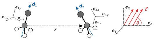
Figure 1: Illustration of two rotating polar molecules with permanent dipole moments $\bm{d}_{1}$ and $\bm{d}_{2}$ interacting with an external dc field $\mathcal{E}$. The laboratory-fixed frame $(X,Y,Z)$ is chosen so that $\bm{r}=r\bm{e}_{Z}$. In addition, each molecule has an associated molecule-fixed frame $(x_{i},y_{i},z_{i})$. Note that we illustrate two prolate symmetric tops with $\bm{d}_{i}=d_{i}\bm{e}_{i,z}$, but we can employ other choices.

II.1 Hamiltonian

The Hamiltonian describing the system reads as

$$\hat{H}=\hat{H}_{\mathrm{rot}}+\hat{H}_{\mathrm{dc}}+\hat{H}_{\mathrm{dd}}\,,$$ (1)

where $\hat{H}_{\mathrm{rot}}$ describes the rotation of both molecules, $\hat{H}_{\mathrm{dc}}$ describes the interaction with the external electric field, and $\hat{H}_{\mathrm{dd}}$ describes the dipole-dipole interaction. Note that we neglect the effect of internal spin.

Under the rigid rotor approximation, the rotation of the molecules is described by Zare (1988)

$$\hat{H}_{\mathrm{rot}}=\sum_{i=1}^{2}\left(A_{i}\hat{\bm{J}}_{i,a_{i}}^{2}+B_{i}\hat{\bm{J}}_{i,b_{i}}^{2}+C_{i}\hat{\bm{J}}_{i,c_{i}}^{2}\right)\,,$$ (2)

where $A_{i}\geq B_{i}\geq C_{i}$ are the rotational constants of each molecule in their principal axes of inertia $a_{i}$, $b_{i}$, and $c_{i}$, and $\hat{\bm{J}}_{i}=(\hat{J}_{i,a_{i}},\hat{J}_{i,b_{i}},\hat{J}_{i,c_{i}})$ are the angular-momentum operators. The values of the rotational constants define the geometry of the molecule, as detailed in Appendix A.1. We also define the molecule-fixed frame as $(x_{i},y_{i},z_{i})=(a_{i},b_{i},c_{i})$ for oblate symmetric tops, whereas as $(x_{i},y_{i},z_{i})=(b_{i},c_{i},a_{i})$ otherwise Zare (1988). In the following, we work with two molecules of the same species, and therefore we consider $A=A_{1}=A_{2}$, $B=B_{1}=B_{2}$, and $C=C_{1}=C_{2}$, but this assumption could easily be relaxed.

The interaction between the permanent dipoles and the external field is described by

$$\hat{H}_{\mathrm{dc}}=-\sum_{i=1}^{2}\hat{\bm{d}}_{i}\cdot\bm{\mathcal{E}}\,,$$ (3)

where $\hat{\bm{d}}_{i}$ is the dipole-moment operator and $\bm{\mathcal{E}}=\mathcal{E}(\cos\theta\,\bm{e}_{Z}+\sin\theta\,\bm{e}_{X})$ is an external dc field. The laboratory-fixed frame $(X,Y,Z)$ is chosen such that the vector connecting the two molecules is defined by $\bm{r}=r\bm{e}_{Z}$, and thus $\theta$ is the angle between $\mathcal{E}$ and the $YZ$-plane (see figure 1).

Finally, the dipole-dipole interaction is described by

$$\hat{H}_{\mathrm{dd}}=\frac{(\hat{\bm{d}}_{1}\cdot\hat{\bm{d}}_{2})-3(\hat{\bm{d}}_{1}\cdot\bm{e}_{\bm{r}})(\hat{\bm{d}}_{2}\cdot\bm{e}_{\bm{r}})}{r^{3}}\,,$$ (4)

where $\bm{e}_{\bm{r}}=\bm{e}_{Z}$ in our chosen frame. Note that we work in units of $\epsilon_{0}=1/4\pi$, where $\epsilon_{0}$ is the vacuum permittivity. In order to work with the standard rotational basis set, we recast the dipole-dipole interaction in terms of spherical tensors Zare (1988); Man (2013), enabling us to write $\hat{H}_{\mathrm{dd}}$ as Krems (2019)

$$\hat{H}_{\mathrm{dd}}=-\frac{\sqrt{6}}{r^{3}}\sum_{p=-2}^{2}(-1)^{p}C^{(2)}_{-p}(\Omega_{r})[\hat{\bm{d}}_{1}\otimes\hat{\bm{d}}_{2}]^{(2)}_{p}\,,$$ (5)

where $\Omega_{r}=(\theta_{r},\phi_{r})$ denotes the polar and azimuthal angles between $\bm{r}$ and the laboratory-fixed frame, $C^{(2)}_{p}$ is an unnormalised spherical harmonic [see Eq. (22)], and

$$[\bm{d}_{1}\otimes\bm{d}_{2}]^{(2)}_{p}=\sum_{p^{\prime}=-1}^{1}\innerproduct{1\,p^{\prime},1\,p-p^{\prime}}{2\,p}d_{1,p^{\prime}}d_{2,p-p^{\prime}}\,,$$ (6)

is the rank-2 tensor product between the two dipole moments, with $\innerproduct{l_{1}\,m_{1},l_{2}\,m_{2}}{l_{3}\,m_{3}}$ the Clebsch–Gordan coefficients. Note that the dipoles have been expressed in their rank-1 spherical tensor form $d_{0}=d_{Z}$ and $d_{\pm 1}=\mp(d_{X}\pm i\,d_{Y})/\sqrt{2}$. We refer to appendix A.2 for complete details on the spherical tensor formalism.

In our chosen laboratory-fixed frame we have that $\Omega_{r}=(\theta_{r},\phi_{r})=(0,0)$, and thus only the $p=0$ term in Eq. (5) contributes. Therefore, we obtain the simpler expression Wall et al. (2015); Dawid et al. (2018)

$$\hat{H}_{\mathrm{dd}}=-\frac{1}{r^{3}}\left(2d_{1,0}d_{2,0}+d_{1,-1}d_{2,1}+d_{1,1}d_{2,-1}\right)\,.$$ (7)

We stress that these dipole elements $d_{i,p}$ are expressed in the laboratory-fixed frame and need to be transformed to their known values in the molecule-fixed frame. This is easily done by using spherical tensor transformations [see Eq. (19)].

II.2 Symmetric top basis and diagonalisation

To diagonalise the Hamiltonian, we work in terms of a basis set

$$\ket{\alpha}\equiv\ket{j_{1}\,k_{1}\,m_{1},j_{2}\,k_{2}\,m_{2}}\,,$$ (8)

where $\ket{j_{i}\,k_{i}\,m_{i}}$ are the usual symmetric top wavefunctions for each molecule Zare (1988) which characterise their rotational state. Indeed, the square of the molecule’s angular momentum $\hat{\bm{J}}_{i}^{2}$ has the usual quantisation $j_{i}(j_{i}+1)$ with $j_{i}=0,1,...$, whereas the projection on the laboratory-fixed axis $J_{Z}$ is quantised by $-j_{i}\leq m_{i}\leq j_{i}$. The additional quantum number $k_{i}$ denotes the quantisation of the projection on the molecule-fixed axis $J_{z_{i}}$. For linear molecules it can be discarded ($k=0$), while for non-linear molecules it takes values $-j_{i}\leq k_{i}\leq j_{i}$. We provide a detailed presentation of this basis in Appendix A.

To diagonalise the problem numerically we construct a basis set with Fock states up to a chosen cutoff $j_{\mathrm{max}}$ for both $j_{i}$. We then construct the Hamiltonian matrix in this truncated subspace and perform the diagonalisation with standard numerical routines for sparse matrices. In this work, we employ a cutoff of $j_{\mathrm{max}}=7$, which enables us to safely study the lower part of the energy spectrum Dawid and Tomza (2020). We provide the explicit expressions for the matrix elements in Appendix B. We also examine the convergence of the calculations as a function of $j_{\mathrm{max}}$ in Appendix C.

II.3 Molecules under consideration

Throughout this article, we consider three types of molecules. First, we consider linear molecules, such as CaF and RbCs, with permanent dipole moments $\bm{d}_{i}=d\bm{e}_{z_{i}}$. Because we scale the results in terms of the parameters of the problem, our results are independent of the specific linear molecule in consideration. Second, we consider fluoroform (CHF₃), an oblate symmetric top. Finally, we consider 1,2-propanediol (CH3CHOHCH2OH), a near-prolate chiral asymmetric top molecule. We note that both CHF₃ and 1,2-propanediol are not amongst the current candidates for cooling to ultracold temperatures in the $\mu$K regime and below. However, their properties are well-known and the values of their rotational constants are convenient to visualise their low-energy properties in this theoretical study. Nevertheless, both molecules can still be cooled to the $\sim$K regime Strebel et al. (2010); Patterson and Doyle (2012).

We provide the rotational constants and components of the dipole moment in table 1. We stress that while the opposite enantiomers of 1,2-propanediol have components $d_{c}$ with opposite signs, the choice of enantiomers does not affect our calculations because we do not consider any enantio-discriminatory element in our model.

Table 1: Molecular properties of CHF₃ Schoolery and Sharbaugh (1951); Meerts and Ozier (1981) and 1,2-propanediol Lovas et al. (2009). The rotational constants ($A$, $B$, $C$) are given in GHz, whereas the dipole moments ($d_{a}$, $d_{b}$, $d_{c}$) are given in Debye. Note that opposite enantiomers ($R$ and $S$) of 1,2-propanediol have $d^{(R)}_{c}=-d^{(S)}_{c}$.

Molecule	$A$	$B$	$C$	$d_{a}$	$d_{b}$	$d_{c}$
CHF3	10.348	10.348	5.6734	0	0	1.645
1,2-propanediol	8.57205	3.640	2.790	1.2	1.9	$\pm$ 0.36

III Zero external field

We start by examining the behaviour of two interacting polar molecules in the absence of external fields. This enables us to quantify the impact of the dipole-dipole interaction on the rotational states.

In figure 2 we show the low-energy spectrum $E$ as a function of the distance between molecules $r$ for the three types of molecules considered in this work. We scale the energies in terms of the rotational constant $B$ of each molecule and their separation in terms of the characteristic distance $r_{B}=(d^{2}/B)^{1/3}$ Micheli et al. (2007); Wall and Carr (2009), where $d=\norm{\bm{d}}$. This characteristic distance separates the regime where the system is dominated by the dipole-dipole interaction $r\ll r_{B}$ to that dominated by the rotational excitations $r\gg r_{B}$. It is usually of the order of tens of nanometres Wall and Carr (2009), smaller than the average separation of current molecular dipolar gases Ni et al. (2008). Nevertheless, examining this regime enables us to better characterise the spectrum and could also be relevant when constructing effective dipolar interactions. We also note that the spectrum for linear molecules [panel (a)] has been examined previously in Ref. Micheli et al. (2007). In this figure (and all the subsequent ones) we have highlighted the lowest-energy states to aid readability.

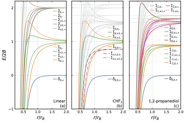
Figure 2: Low-energy spectrum as a function of $r$ for two linear (a), CHF₃ (b), and 1,2-propanediol (c) molecules in the absence of external fields. Solid lines correspond to symmetric solutions, dashed lines correspond to antisymmetric solutions, and dash-dotted states correspond to degenerate solutions of symmetric and antisymmetric states. The thin horizontal lines correspond to the known energies of two independent rotating molecules [see Appendix A], while the vertical lines indicate $r=r_{B}$. The labelling convention is explained in the main text.

We first stress that at large distances $r\gg r_{B}$ the molecules decouple, and thus we recover the known spectrum for two non-interacting rotating molecule (as examined in Appendix A.1), as expected. Indeed, for $r\gg r_{B}$, the ground states in figure 2 simply correspond to two molecules in their $j_{i}=0$ state, the subsequent excited states correspond to one molecule in its first excited $j_{1/2}=1$ state with the other in its ground $j_{2/1}=0$ state, and so on. These known energy values are shown as the thin horizontal lines.

For shorter distances $r\lesssim r_{b}$, as shown in Ref. Micheli et al. (2007) for linear molecules, we observe that the dipole-dipole interaction plays a significant role, changing the energy spectrum and breaking degeneracies. Nevertheless, the symmetries of the Hamiltonian enable us to characterise the different energy levels. Indeed, while the dipole-dipole interaction mixes states with different $j=j_{1}+j_{2}$, both $m=m_{1}+m_{2}$ and $k=k_{1}+k_{2}$ are conserved. Moreover, because the Hamiltonian is invariant under the exchange of the two molecules, the solutions can either be symmetric ($+$) or antisymmetric ($-$), which we denote via $P$. Thus the full labelling system is: $\bar{j}_{m,P}$ for linear molecules, $\bar{j}_{k,m,P}$ for symmetric molecules, and $\bar{j}_{\bar{\tau},m,P}$ for asymmetric molecules. Here $\bar{j}$ corresponds to the value of $j$ in the limit $r\to\infty$. Similarly, $\bar{\tau}$ corresponds to the value of the pseudo-quantum number $\tau=\tau_{1}+\tau_{2}$ which labels the states of asymmetric tops (see Appendix A.1). We note that here and in the following we use overbars to denote labels that do not correspond to good quantum numbers.

First, for linear tops (a) we observe that as $r$ decreases, the energy levels separate into symmetric (solid lines) and antisymmetric (dashed lines) solutions with a constant $\absolutevalue{m}$. Therefore, the levels with $m=0$ are not degenerate, whereas the $|m|>0$ levels are twice degenerate. The gaps between the energy levels become more prominent around $r\approx r_{B}$, at which point some energy levels increase with decreasing $r$, while others decrease. However, all the energy levels diverge to $E_{\bar{j},m,P}\to-\infty$ deep in the molecular region $r\ll r_{B}$ Micheli et al. (2007) as a consequence of the diverging nature of the dipole-dipole interaction for $r\to 0$.

The energy spectrum of symmetric tops (b) has a similar structure to that of linear tops. The spectrum shows symmetric and antisymmetric solutions, and solutions with constant $\absolutevalue{m}$ and $|k|$. The solutions for $k=0$ simply correspond to the spectrum of linear tops (see blue, orange, and green lines) because symmetric tops do not mix states with different $k$. On the other hand, the solutions for $k\neq 0$ add additional states between those for $k=0$. Note that because we examine an oblate top, the states with $k\neq 0$ have less energy than that for $k=0$. In contrast, states with $k\neq 0$ in prolate tops increase the energy (see Eq. 16). Interestingly, the states with $k\neq 0$ have degenerate symmetric and antisymmetric solutions (dash-dotted lines). Therefore, the states $\bar{1}_{\pm 1,\pm 1}$ (purple lines) are eightfold degenerate, while the states $\bar{1}_{\pm 1,0}$ (red lines) are fourfold degenerate.

Finally, the energy spectrum of asymmetric tops (c) shows similar features to the previous spectra, but with much more energy states. Because asymmetric tops mix states with different $k$, the solutions are only labelled by the pseudo-quantum number $\tau$ (see Appendix A.1 for details), and no state coincides with states of linear molecules. Indeed, despite being similar, even the ground state (blue line) of two asymmetric tops is slightly different to that of linear molecules. In addition, asymmetric tops show fewer degenerate states than symmetric tops, as only states with $m\neq 0$ are twice degenerate, with no degenerate symmetric and antisymmetric states.

Because the spectrum of two interacting asymmetric tops depends on the rotational constants, the control of the separation between interacting molecules, for example with optical tweezers, could be employed to experimentally measure the moments of inertia, which are generally difficult to characterise. Moreover, the use of external fields, as in the next section, provides additional parameters to control for molecular measurements. We provide additional details about the dependence of the energy spectrum of asymmetric molecules on their geometry in Appendix D.

IV Finite external field

We now turn our attention to the problem of two interacting polar molecules in the presence of an external dc electric field $\bm{\mathcal{E}}$. We continue our examination of the energy spectrum, and we also examine the total expectation value of the projection of the dipole moments on a laboratory axis $L=X,Y,Z$,

$$\expectationvalue{d_{L}}=\expectationvalue{d_{1,L}+d_{2,L}}/2\,.$$ (9)

The expectation values are calculated from the obtained eigenvectors (for more details see Appendix A.3). In the following, we separate our discussion again into linear, symmetric, and asymmetric molecules.

IV.1 Linear tops

We start by examining the behaviour of the molecules interacting with a fixed external field as a function of their separation, expanding on the spectrum shown in figure 2. In figure 3 we report the energy spectrum and average projection of the dipole moment on the laboratory-frame axes as a function of the distance. We consider an external field in the $\bm{e}_{Z}$ direction in the left panels, and a field in the $\bm{e}_{X}$ direction in the right panels. Because the molecules develop a finite dipole projection only in the direction of the dc field, we only show $\expectationvalue{d_{Z}}$ and $\expectationvalue{d_{X}}$ for the fields in the $\bm{e}_{Z}$ and $\bm{e}_{X}$ directions in panels (c) and (d), respectively. We also only show the dipole projections of the highlighted states in the energy spectrum. Note that all the results converge to the known single molecule limits (thin horizontal lines) for $r\gg r_{B}$, as expected.

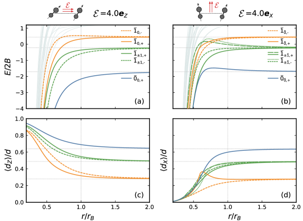
Figure 3: Low-energy spectrum (a,b) and average dipole moment projection on the $\bm{e}_{Z}$ (c) and $\bm{e}_{X}$ (d) axes of two linear molecules as a function of the distance between molecules $r$. The left panels (a,c) consider an external dc field $\bm{\mathcal{E}}=4.0\bm{e}_{Z}$, whereas the right panels (b,d) consider an external dc field $\bm{\mathcal{E}}=4.0\bm{e}_{X}$. Lines with the same colour and line type in the upper and bottom panels indicate the same eigenstate. The thin horizontal lines correspond to the known energies of two independent rotating molecules interacting with a dc field of magnitude $\mathcal{E}=4.0$, while the vertical lines indicate $r=r_{B}$. The labelling convention is explained in the main text.

We first note that the symmetries of the Hamiltonian undergo an important change as the direction of the electric field is varied. While $m$ is conserved for fields in the $\bm{e}_{Z}$ direction, this symmetry is broken if the dc field has a component in any other direction. We can understand this by noting that the dipole-dipole interaction conserves the projection of the angular momentum in the direction of $\bm{r}$, which corresponds to $\bm{e}_{Z}$ in our case. Therefore, the dipole-dipole interaction conserves $m$, as discussed in the previous section. On the other hand, the electric field conserves the projection of the angular momentum in the direction of the field. Therefore, $m$ is only conserved if the electric field is in the $\bm{e}_{Z}$ direction. In any other case, there is a competition between the electric field and dipole-dipole interaction which breaks this symmetry. Due to this, we label the eigenstates in the left panels as $\bar{j}_{m,P}$ as in section III, whereas we label the states in the right panels as $\bar{j}_{\bar{m},P}$ where $\bar{m}$ gives the value of $m$ in the limit $r\gg r_{B}$. However, we stress that around the molecular region ($r\approx r_{B}$) the value of $\bar{m}$ is only a label, rather than a good quantum number.

Another interesting consequence of the direction of the field is the breaking of degeneracies. While for fields in the $\bm{e}_{Z}$ direction the two pairs of states with equal $\absolutevalue{m}$ are degenerate as with no external field (see the two green lines in the left panels of figure 3), this degeneracy is broken if the field has a component in any other direction (see the four green lines in the right panels). This behaviour has been already reported and discussed in Ref. Micheli et al. (2007).

Concerning the dipole projections, in all cases, $\expectationvalue{d_{L}}$ converges to the expected single molecule solution for $r\gg r_{B}$. However, $\expectationvalue{d_{L}}$ behaves significantly differently at short distances depending on the direction of the fields. While $\expectationvalue{d_{Z}}$ increases at short distances for fields in the $\bm{e}_{Z}$ direction (c), $\expectationvalue{d_{Z}}$ instead decreases at short distances for fields in the $\bm{e}_{X}$ direction (d), vanishing for $r\to 0$. To interpret this, we recall that the dipole-dipole interaction becomes maximally attractive for dipoles polarised in the direction of $\bm{r}$, whereas it becomes maximally repulsive for dipoles polarised orthogonal to $\bm{r}$. Therefore, considering that the external field tries to polarise the dipoles in the direction of $\bm{\mathcal{E}}$, the dipole-dipole interaction enhances the polarisation at short distances if the field is in the $\bm{e}_{Z}$ direction. In contrast, for fields in the $\bm{e}_{X}$ direction, it is not favourable to have dipoles polarised in the $\bm{e}_{X}$ direction at short distances due to the repulsive nature of the dipole-dipole interaction. This drives $\expectationvalue{d_{X}}$ to vanish for $r\to 0$. This effect could be relevant to take into account in molecular dipolar gases under weak electric fields.

Finally, to further examine the behaviour of the molecules interacting with dc fields in different directions, we show the energy spectrum and dipole projections as a function of $\theta$ in figure 4. We choose a fixed magnitude $\mathcal{E}$ and distance $r=r_{B}$ between molecules. The figure connects the field in the $\bm{e}_{Z}$ direction ($\theta=0^{\circ}$) to the field in the $\bm{e}_{X}$ direction ($\theta=90^{\circ}$). The energy spectrum shows how the presence of components of $\bm{\mathcal{E}}$ orthogonal to $\bm{e}_{Z}$ breaks the degeneracy of states with equal $\absolutevalue{m}$. Indeed, the two green lines at $\theta=0$ smoothly separate into four lines as $\theta$ increases. In addition, the spectrum shows how the eigenstates are connected between the two limits, which is the reason for the particular colour scheme used in figure 3. Moreover, the figure shows clearly that the direction of the dc field also affects the energies of the level themselves. Indeed, even the ground state energy depends on $\theta$.

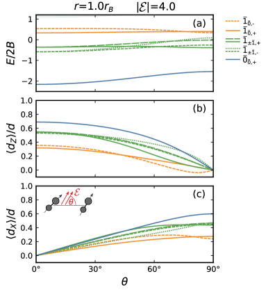
Figure 4: Low-energy spectrum (a) and average dipole moment projections $\expectationvalue{d_{Z}}$ (b) and $\expectationvalue{d_{X}}$ (c) for two linear molecules as a function of the angle $\theta$ between $\bm{\mathcal{E}}$ and the YZ-plane. We consider a distance $r=r_{B}$ and a field of magnitude $\mathcal{E}=4.0$. Lines with the same colour and line type in the upper and bottom panels indicate the same eigenstate. The labelling convention is explained in the main text.

Figure 4 also shows how the dipole moment projections depend on the direction of the external field, with $\expectationvalue{d_{Z}}$ developing an increasing finite value as $\theta\to 0$, whereas $\expectationvalue{d_{X}}$ instead develops a finite value as $\theta\to 90^{\circ}$. We also note that $\langle d_{X}\rangle|_{\theta=90^{\circ}}<\langle d_{Z}\rangle|_{\theta=0^{\circ}}$ for the same eigenstate, due to the enhancement of the dipole projection for fields in the direction of $\bm{r}$, as discussed previously.

IV.2 Symmetric tops

We now extend our previous examination to the oblate symmetric top. We show the energy spectrum and dipole moment projections as a function of the distance between CHF₃ molecules in figure 5, considering again electric fields in the $\bm{e}_{Z}$ and $\bm{e}_{X}$ directions. Naturally, the features observed with linear molecules are largely carried over to more complex molecules. Indeed, $m=m_{1}+m_{2}$ is only conserved if the dc field is in the direction of $\bm{r}$. However, the projection of the angular momentum onto the molecular axis, $k$, remains conserved in all cases. This can be expected, as the molecule-fixed axes simply move alongside the molecules and do not depend on the direction of the interactions. Therefore, we label the states as $\bar{j}_{k,m,P}$ for fields in the $\bm{e}_{Z}$ direction, and $\bar{j}_{k,\bar{m},P}$ otherwise, where $\bar{m}$ gives the value of $m$ for $r\gg r_{B}$.

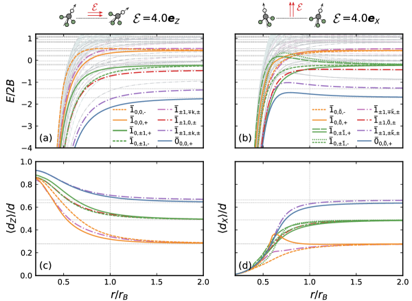
Figure 5: Low-energy spectrum (a,b) and average dipole moment projection on the $\bm{e}_{Z}$ (c) and $\bm{e}_{X}$ (d) axes of two CHF₃ molecules as a function of the distance between molecules $r$. The left panels (a,c) consider an external dc field $\bm{\mathcal{E}}=4.0\bm{e}_{Z}$, whereas the right panels (b,d) consider an external dc field $\bm{\mathcal{E}}=4.0\bm{e}_{X}$. Lines with the same colour and line type in the upper and bottom panels indicate the same eigenstate. The thin horizontal lines correspond to the known energies of two independent rotating molecules interacting with a dc field of magnitude $\mathcal{E}=4.0$, while the vertical lines indicate $r=r_{B}$. The labelling convention is explained in the main text.

The dipole projections also behave as they do with linear molecules, as expected. We observe that $\expectationvalue{d_{Z}}$ increases at short distances for fields in the $\bm{e}_{Z}$ direction, whereas $\expectationvalue{d_{Z}}$ decreases for fields in the $\bm{e}_{X}$ direction. In addition, the states with $k=0$ are identical to those of linear molecules, as there is no mixing of states with different $k$. Nevertheless, the states with $k\neq 0$ fill the energy spectrum with additional states. Again, we only highlight in colour the states with $\bar{j}=0,1$.

As seen with no external fields, the states with $k\neq 0$ generally have degenerate symmetric and asymmetric solutions. This degeneracy is not necessarily broken by the introduction of external fields. Indeed, the highlighted excited states (red and purple lines) maintain this degeneracy. However, we have observed that other states can have this degeneracy broken. The external field does separate states with $k=\pm m$ and $k=\mp m$ (compare purple lines in figure 6 with that in figure 2b). This is simply induced by the Stark effect, as shown for single molecules in figure 10b.

Finally, we show the spectrum and dipole projections as a function of $\theta$ in figure 6. All the eigenstates show a smooth crossover between the $\theta=0$ and $\theta=90^{\circ}$ limits, with $\expectationvalue{d_{X}}$ vanishing for $\theta\to 0$, and $\expectationvalue{d_{Z}}$ vanishing for $\theta\to 90^{\circ}$. The states with $k\neq 0$ do not show any unexpected behaviour as $\theta$ changes.

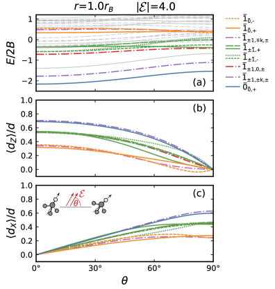
Figure 6: Low-energy spectrum (a) and average dipole moment projections $\expectationvalue{d_{Z}}$ (b) and $\expectationvalue{d_{X}}$ (c) for two CHF₃ molecules as a function of the angle $\theta$ between $\bm{\mathcal{E}}$ and the YZ-plane. We consider a distance $r=r_{B}$ and a field of magnitude $\mathcal{E}=4.0$. Lines with the same colour and line type in the upper and bottom panels indicate the same eigenstate. The labelling convention is explained in the main text.

IV.3 Asymmetric tops

We finish our examination of molecules interacting with external dc fields by considering asymmetric tops. We show the spectrum and dipole projections of two 1,2-propanediol molecules as a function of the separation between them in figure 7. We consider the same fields as in the previous figures. The overall behaviour of the energy spectrum and dipole projections is similar to that of symmetric and linear tops, with the states converging to the known single molecule solutions for $r\gg r_{B}$ and with $m$ being a good quantum number only for fields in the $\bm{e}_{Z}$ direction. Similarly, $\expectationvalue{d_{Z}}$ is enhanced at short distances for fields in the $\bm{e}_{Z}$ direction, whereas $\expectationvalue{d_{X}}$ vanishes at short distances for fields in the $\bm{e}_{X}$ direction. Therefore, we label the states as $\bar{j}_{\bar{\tau},\bar{m},P}$, extending our previous conventions. Nevertheless, asymmetric tops show a more complex behaviour with additional states, which can be expected from the mixing of states with different values of $k$.

Figure 7: Low-energy spectrum (a,b) and average dipole moment projection on the $\bm{e}_{Z}$ (c) and $\bm{e}_{X}$ (d) axes of two 1,2-propanediol molecules as a function of the distance between molecules $r$. The left panels (a,c) consider an external dc field $\bm{\mathcal{E}}=4.0\bm{e}_{Z}$, whereas the right panels (b,d) consider an external dc field $\bm{\mathcal{E}}=4.0\bm{e}_{X}$. Lines with the same colour and line type in the upper and bottom panels indicate the same eigenstate. The thin horizontal lines correspond to the known energies of two independent rotating molecules interacting with a dc field of magnitude $\mathcal{E}=4.0$, while the vertical lines indicate $r=r_{B}$. The labelling convention is explained in the main text.

As with no external field, and in contrast to symmetric tops, asymmetric molecules do not show degenerate symmetric and asymmetric states and instead, they are noticeably distinguishable for $r\lesssim r_{B}$. Some states also show prominent jumps in the dipole projections (see for example solid orange and pink lines in panel c) due to avoided crossings in the spectra Yu et al. (2019). We have found that as the molecules move closer (for $r\lesssim r_{B}$) and many levels have similar energies, there is a strong mixing of Fock states with different $j$ due to the dipole-dipole interaction and of different $k$ due to the rotation of the asymmetric molecules. This mixing produces noticeable variations in the eigenvectors, and thus in the dipole projections. We stress again that the numbers we have associated with each state are only meaningful at $r\gg r_{B}$, and at shorter distances, they only act as labels of each quantum state.

Finally, we show the spectrum and dipole projections of two 1,2-propanediol molecules as a function of $\theta$ in figure 8. The molecules show the expected behaviour, with a smooth crossover between fields in the $\bm{e}_{Z}$ and $\bm{e}_{X}$ limits. The additional complexity of asymmetric tops becomes maybe more noticeable, with a less clear difference in the dipole projections between states. In addition, avoided crossings with jumps in $\langle d\rangle$ also occur as $\theta$ changes.

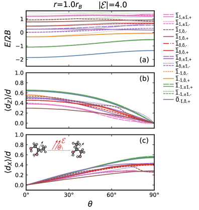
Figure 8: Low-energy spectrum (a) and average dipole moment projections $\expectationvalue{d_{Z}}$ (b) and $\expectationvalue{d_{X}}$ (c) for two 1,2-propanediol molecules as a function of the angle $\theta$ between $\bm{\mathcal{E}}$ and the YZ-plane. We consider a distance $r=r_{B}$ and a field of magnitude $\mathcal{E}=4.0$. Lines with the same colour and line type in the upper and bottom panels indicate the same eigenstate. The labelling convention is explained in the main text.

The mentioned additional complexity of asymmetric tops and high level of near degeneracy makes them less suitable candidates for molecular control. In particular, symmetric tops are probably much better options for quantum computing applications due to having better-defined properties Yu et al. (2019). Nevertheless, a good understanding of the rotational properties of asymmetric molecules can be important for enantio-discrimination of cold chiral molecules Tutunnikov et al. (2018). In this direction, a more comprehensive study of the states of asymmetric molecules is needed, which is left for future work.

V Conclusions

We have investigated the behaviour of two rotating polar molecules interacting via the dipole-dipole interaction and with an external dc electric field. We presented a comprehensive examination of the energy spectra and polarisation of the dipoles for linear, symmetric and asymmetric top molecules. The account of molecular rotation results in rich behaviour at short inter-molecular distances, with a strong dependence on both the direction of the external field and the separation. The molecules examined largely share a similar behaviour, with symmetric and asymmetric molecules adding an increasing complexity, resulting in a high number of states with similar energies and dipole projections at short separations.

We found that the dipole projection on the direction of the electric field becomes enhanced at short separation if the field is in the direction of the vector connecting the molecules, resulting in a stronger polarisation. In contrast, for fields orthogonal to the molecules’ plane, at short separations, it is not favourable to have dipoles polarised in the direction of the field due to the strong repulsive dipole-dipole interaction. While these effects arise at very short separations, these might be relevant to account in many-body applications of polar molecules when building effective dipole-dipole interactions. More generally, the account of rotation in many-body applications of polar molecules could be exploited to achieve new forms of quantum matter not realisable by single atoms, as also suggested by related few-body works on rotating diatomic molecules Dawid et al. (2018); Dawid and Tomza (2020).

The rich behaviour shown by the molecules, especially at short separations, could be also relevant to consider when proposing polar molecules as qubit storage Gregory et al. (2021), as the dipole-dipole interaction plays an important role in designing the corresponding quantum gates Ni et al. (2018). In particular, qubits constructed with symmetric tops have been proposed Wei et al. (2011), which rely on having opposite dipole projections for states with $k=\pm 1$. Therefore, precise control of the dipoles polarisation is required for designing quantum computing platforms Yu et al. (2019).

Future work will consider additional effects, such as from hyperfine structure and interactions with external magnetic and ac electric fields Krems (2019). We also intend to consider mobile molecules trapped in harmonic traps, as studied for two molecules in Refs. Dawid et al. (2018); Dawid and Tomza (2020), with the final aim of describing more realistic many-body configurations. Similarly, we intend to study polar molecules immersed in lattice configurations, complementing recent efforts to describe non-reactive molecules in optical lattices Doçaj et al. (2016); Wall et al. (2017). In this direction, it will be particularly interesting to examine non-linear molecules to further describe recently proposed scenarios of symmetric and asymmetric molecules trapped in lattice configurations Yu et al. (2019); Isaule et al. (2022).

Appendix A Single-molecule physics

In the following, we summarise the description of a single rotating polar molecule for readers unfamiliar with rotating molecules and spherical tensors. For comprehensive reviews, we refer to Refs. Zare (1988); Krems (2019); Di Lauro (2020).

A.1 Rotational Hamiltonian

The Hamiltonian describing a single rigid rotor reads

$$\hat{H}_{\mathrm{rot}}=\left(A\hat{\bm{J}}_{a}^{2}+B\hat{\bm{J}}_{b}^{2}+C\hat{\bm{J}}_{c}^{2}\right)\,.$$ (10)

The rotational constants are defined from the principal moments of inertia $I_{a}$, $I_{b}$, $I_{c}$, as $A=\hbar/(4\pi I_{a})$, $B=(\hbar/4\pi I_{b})$, and $C=(\hbar/4\pi I_{c})$, so have the units of frequency. The values of the rotational constants define the geometry of the molecule. Indeed, all molecules can be classified as

$$I_{a}=0,\,I_{b}=I_{c}>0\quad \textrm{: Linear top}\,,$$

$$I_{a}=I_{b}=I_{c}\quad \textrm{: Spherical top}\,,$$

$$I_{a}=I_{b}<I_{c}\quad \textrm{: Oblate symmetric top}\,,$$

$$I_{a}<I_{b}=I_{c}\quad \textrm{: Prolate symmetric top}\,,$$

$$I_{a}<I_{b}<I_{c}\quad \textrm{: Asymmetric top}\,.$$

Diatomic and some triatomic molecules are linear tops, while many small polyatomic molecules, such as CH₃F and CaOCH₃ are symmetric tops. However, most polyatomic molecules are asymmetric tops, even though some can approximately be treated as near symmetric.

To diagonalise (10), one generally works in terms of the symmetric top wavefunctions $\ket{j\,k\,m}$, where $j=0,1,...$, $-j\leq k\leq j$, and $-j\leq m\leq j$.. These are defined as

$$\innerproduct{\Omega}{j\,k\,m}=\sqrt{\frac{2j+1}{8\pi}}D^{j*}_{m,k}(\Omega),$$ (11)

where here $\Omega=(\phi,\theta,\chi)$ denotes the Euler angles between the molecule- and laboratory-fixed frames, and $D^{j}_{m,k}(\Omega)$ are the Wigner $D$-matrices Zare (1988). In the $\ket{j\,k\,m}$ basis, the angular momentum operator satisfies

$$\hat{\bm{J}}^{2}\,\ket{j\,k\,m} =j(j+1)\,\ket{j\,k\,m}\,,$$ (12)

$$\hat{J}_{z}\,\ket{j\,k\,m} =k\,\ket{j\,k\,m}\,,$$ (13)

$$\hat{J}_{Z}\,\ket{j\,k\,m} =m\,\ket{j\,k\,m}\,.$$ (14)

As illustrated in figure 9, $k$ represents the projection of the angular moment onto the molecule-fixed frame, whereas $m$ represents the usual projection onto the laboratory-fixed frame. Therefore, $\ket{j\,k\,m}$ enables one to identify the rotational state of the molecule. Note that, as explained in the main text, for symmetry arguments we define $(x,y,z)=(a,b,c)$ for oblate symmetric tops, whereas as $(x,y,z)=(b,c,a)$ otherwise Zare (1988). Also note that linear molecules cannot rotate on their $a$-axis, so we can simply consider $k=0$.

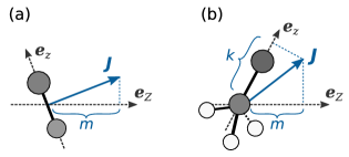
Figure 9: Illustration of a rotating linear (a) and prolate symmetric (b) top molecule with angular momentum $\bm{J}$ with respect to the laboratory-fixed axis $\bm{e}_{Z}$ and the molecule-fixed axis $\bm{e}_{z}$.

In the case of linear and spherical tops, it is easy to see that the rotating Hamiltonian is simply

$$\hat{H}_{\mathrm{rot}}=B\hat{\bm{J}}^{2}\,,$$ (15)

resulting in the well-known spectrum $E_{j}=Bj(j+1)$. In the case of prolate tops, the Hamiltonian can be written as

$$\hat{H}_{\mathrm{rot}}=C\hat{\bm{J}}^{2}+(A-C)\hat{\bm{J}}_{z}^{2}\,.$$ (16)

From Eqs. (12) and (13), one sees that $\hat{H}_{\mathrm{rot}}$ is diagonal in $\ket{j\,k\,m}$, resulting in the spectrum $E_{j,k}=Cj(j+1)+(A-C)k^{2}$. Similarly, for oblate tops one simply exchanges $A$ by $C$ in Eq. (16), resulting in $E_{j,k}=Aj(j+1)+(C-A)k^{2}$.

Finally, asymmetric tops do not have $\hat{H}_{\mathrm{rot}}$ diagonal in $\ket{j\,k\,m}$. Indeed, the non-zero elements of the Hamiltonian matrix are given by

$$\langle j\,k\,m|\hat{H}_{\mathrm{rot}}|j\,k\,m\rangle =\frac{B+C}{2}\left(j(j+1)-k^{2}\right)+A\,k^{2}\,,$$ (17)

$$\langle j\,k\,m|\hat{H}_{\mathrm{rot}}|j\,k\pm 2\,m\rangle =\frac{B-C}{4}f_{\pm}(j,k)\,,$$ (18)

where $f_{\pm}(j,k)=\sqrt{\left[j(j+1)-k(k\pm 1)\right]\left[j(j+1)-(k\pm 1)(k\pm 2)\right]}$. Therefore, the Hamiltonian couples states with $k\pm 2$, requiring a numerical diagonalisation. We refer to Refs. Zare (1988); Koch et al. (2019) for details on the spectrum of asymmetric tops. In addition, because $k$ is not a good quantum number, the wavefunctions of asymmetric tops take the form $\ket{j\,\tau\,m}=\sum_{k}c_{\tau,k}\ket{j\,k\,m}$, where $\tau=k_{a}-k_{c}=-j,...,+j$ is a pseudo-quantum number that labels the states, where $k_{a}=0,..,j$ and $k_{c}=0,...,j$ are the values that $\absolutevalue{k}$ would take in the prolate and oblate limits, respectively Zare (1988).

A.2 Spherical tensors

Because we are interested in interacting rotating molecules, we need to adapt the interaction terms of the Hamiltonian to the $\ket{j\,k\,m}$ basis. This is easily done by using spherical tensors, which enable us to systematically transform vectors between the laboratory- and molecule-fixed frames.

A $\ell$th-rank spherical tensor $T$ has $2\ell+1$ elements with labels $s=-\ell,...,\ell$. Spherical tensors transform as the following Zare (1988)

$$T_{p}^{(\ell)}=\sum_{q=-\ell}^{\ell}D^{\ell*}_{p,q}(\Omega)T_{q}^{(\ell)}\,,\qquad T_{q}^{(\ell)}=\sum_{p=-\ell}^{\ell}D^{\ell}_{p,q}(\Omega)T_{p}^{(\ell)}\,,$$ (19)

where we use $p$ and $q$ to denote elements in the laboratory- and molecule-fixed frame, respectively. The tensor product between two tensors $V$ and $U$ in an arbitrary frame is defined as

$$[V^{(\ell_{v})}\otimes U^{(\ell_{u})}]^{(\ell)}_{s}= \sum_{s_{v},s_{u}}\innerproduct{\ell_{v}\,s_{v},\ell_{u}\,s_{u}}{\ell\,s}V^{(\ell_{v})}_{s_{v}}U^{(\ell_{u})}_{s_{u}}$$

$$= \sum_{s^{\prime}=-\ell}^{\ell}\innerproduct{\ell_{v}\,s^{\prime},\ell_{u}\,s-s^{\prime}}{\ell\,s}V^{(\ell_{v})}_{s^{\prime}}U^{(\ell_{u})}_{s-s^{\prime}}\,,$$ (20)

where $\innerproduct{l_{1}\,m_{1},l_{2}\,m_{2}}{L\,M}$ are Clebsch–Gordan coefficients, and $\ell_{v}$ and $\ell_{u}$ are the ranks of tensors $V$ and $U$, respectively.

In this work, we transform vectors to rank-1 spherical tensors by employing the spherical basis $(\bm{e}_{-1},\bm{e}_{0},\bm{e}_{1})$. In an arbitrary frame with Cartesian coordinates $(x^{\prime},y^{\prime},z^{\prime})$, the unit spherical vectors read

$$\bm{e}_{0}=\bm{e}_{z^{\prime}},\qquad\bm{e}_{\pm 1}=\mp(\bm{e}_{x^{\prime}}\pm i\,\bm{e}_{y^{\prime}})/\sqrt{2}\,.$$ (21)

The $s=-1,0,+1$ spherical elements of a vector $\bm{v}=(v_{x^{\prime}},v_{y^{\prime}},v_{z^{\prime}})$ in this frame are given by $v_{s}=\bm{e}_{s}\cdot\bm{v}=vC^{(1)}_{s}(\Omega_{\bm{v}})$, where

$$C^{(l)}_{m}(\Omega)=D^{l*}_{m,0}(\Omega)=\sqrt{\frac{4\pi}{2l+1}}Y_{l,m}(\Omega)\,,$$ (22)

are the unnormalised spherical harmonics, and $\Omega_{\bm{v}}=(\theta_{\bm{v}},\phi_{\bm{v}})$ denotes the polar and azimuthal angles of $\bm{v}$ in the chosen frame. Therefore, we can simply express the spherical components of $\bm{v}$ as

$$v_{0}=v_{z^{\prime}},\qquad v_{\pm 1}=\mp(v_{x^{\prime}}\pm i\,v_{y^{\prime}})/\sqrt{2}\,.$$ (23)

All the usual vector operations can be defined in terms of spherical tensors Zare (1988). However, in this work, we are only interested in the dot product between two vectors. This takes the simple form

$$\bm{v}^{*}\cdot\bm{u}=\sum_{s=-1}^{1}(-1)^{s}v_{s}u_{-s}\,.$$ (24)

The previous equations enable us to perform all the necessary transformations between frames. Indeed, the rotational state is encoded entirely in the $D$-matrices, which appear from the transformations (19). The matrix elements of the Hamiltonian in the $|j\,k\,m\rangle$ basis are then obtained by using that Zare (1988)

$$\matrixelement{j\,k\,m}{D^{J*}_{M,K}}{j^{\prime}\,k^{\prime}\,m^{\prime}}=(-1)^{m+k}\sqrt{(2j+1)(2j^{\prime}+1)}\begin{pmatrix}j&J&j^{\prime}\\ -m&M&m^{\prime}\end{pmatrix}\begin{pmatrix}j&J&j^{\prime}\\ -k&K&k^{\prime}\end{pmatrix}\,$$ (25)

where the parentheses are the Wigner 3j-symbols. Note that the only nonvanishing matrix elements are those with $m=m^{\prime}+M$ and $k=k^{\prime}+K$.

A.3 Interacting molecule: Stark effect

We now employ the previous definitions to describe a single rotating molecule interacting with an external dc electric field. The system is described by

$$\hat{H}=\hat{H}_{\mathrm{rot}}+\hat{H}_{\mathrm{dc}}\,,$$ (26)

where $\hat{H}_{\mathrm{rot}}$ is given by Eq. (10) and $\hat{H}_{\mathrm{dc}}=-\bm{d}\cdot\bm{\mathcal{E}}$, with $\bm{d}$ the permanent dipole of the molecule and $\bm{\mathcal{E}}$ the chosen electric field. The matrix elements of $\hat{H}_{\mathrm{rot}}$ in $\ket{j\,k\,m}$ are given in A.1. To compute the matrix elements of $\hat{H}_{\mathrm{dc}}$, we write both $\bm{d}$ and $\bm{\mathcal{E}}$ as spherical tensors, resulting in

$$\hat{H}_{\mathrm{dc}} =-\sum_{p=-1}^{1}(-1)^{p}d_{p}\mathcal{E}_{-p}\,,$$ (27)

$$=-\sum_{p,q}(-1)^{p}D^{1*}_{p,q}(\Omega)\,d_{q}\mathcal{E}_{-p}\,.$$ (28)

where in the first line we used Eq. (24) with both tensors in the laboratory-fixed frame, and in the second line we transformed $\bm{d}$ to the molecule-fixed frame using Eq. (19). We stress that $d_{q}$ and $\mathcal{E}_{p}$ are inputs to the calculation. The matrix elements of Eq. (28) then read

$$\matrixelement{j\,k\,m}{\hat{H}_{\mathrm{dc}}}{j^{\prime}\,k^{\prime}\,m^{\prime}}=-\sum_{p,q}(-1)^{p}\,d_{q}\mathcal{E}_{-p}\matrixelement{j\,k\,m}{D^{1*}_{p,q}(\Omega)}{j^{\prime}\,k^{\prime}\,m^{\prime}}\,,$$ (29)

where $\matrixelement{j\,k\,m}{D^{1*}_{p,q}}{j^{\prime}\,k^{\prime}\,m^{\prime}}$ is given by Eq. (25).

We can compute the energy spectrum by diagonalising $\hat{H}$ either numerically, as in this work, or perturbatively for weak fields Krems (2019). In addition, we can compute the average value of the dipole moment projection in some laboratory-frame direction $p$ from $\expectationvalue{d_{p}}=\expectationvalue{d_{p}}{\Psi}$, where $\ket{\Psi}=\sum_{\alpha}c_{\alpha}\ket{j_{\alpha}k_{\alpha}m_{\alpha}}$ is a chosen eigenvector solution. Therefore,

$$\expectationvalue{d_{p}}{\Psi}=\sum_{\alpha,\beta}c^{*}_{\alpha}c_{\beta}\sum_{q}d_{q}\matrixelement{j_{\alpha}k_{\alpha}m_{\alpha}}{D^{1*}_{p,q}(\Omega)}{j_{\beta}k_{\beta}m_{\beta}}\,,$$ (30)

where $d_{q}$ are the known elements of the dipole moment in the molecule-fixed frame. After computing $\expectationvalue{d_{p}}$, we can extract the projections in cartesian coordinates $(X,Y,Z)$ by using Eq. (23).

We show textbook examples Krems (2019); Wall et al. (2013) of the low-energy spectrum and dipole projection as a function of the external dc field in figure 10. We only highlight the lower-energy states for readability. As in the main text, we show examples for linear molecules, the oblate symmetric top CHF₃ and 1,2-propanediol. We choose a dc field $\bm{\mathcal{E}}=\mathcal{E}\bm{e}_{Z}$, and so the projection of the dipole moment is only finite on the $Z$-axis. However, we stress that for a single rotating molecule, the chosen direction of $\bm{\mathcal{E}}$ is arbitrary.

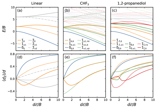
Figure 10: Energy spectrum (a,b,c) and average projection of the dipole moment onto the $\bm{e}_{Z}$ axis (d,e,f) as a function of the magnitude of the external electric field. In the figure $d=|\bm{d}|$ and $B$ is the rotational constant in the $b$-axis. Panels (a,d) show results for a linear molecule, (b,e) show results for CHF₃, and (c,f) show results for 1,2-propanediol.

We label the states as $\bar{j}_{m}$ for linear molecules (a), as $\bar{j}_{k,m}$ for symmetric molecules (b), and as $\bar{j}_{\bar{\tau},m}$ for asymmetric molecules (c), where $j$ is the eigenvalue of $\bm{J}^{2}$ for $\mathcal{E}=0$ and $\tau$ is the pseudo-quantum number relevant to asymmetric tops. Note that while $m$ remains conserved for finite electric fields, $\hat{H}_{\mathrm{dc}}$ couples states with different $j$ Krems (2019).

For $\mathcal{E}=0$, the spectrum is that of a non-interacting rotating molecule described in A.1. With a finite $\mathcal{E}$, the spectrum shows the usual Stark effect, with a splitting of the rotational states. Naturally, symmetric and asymmetric tops show a much richer spectrum due to the additional projection $k$. Note that the lines with finite values of $k$ (or $\tau$) and $m$ are twice degenerate, with solutions where $k$ and $m$ having equal signs (denoted by $\pm m$) and solutions where $k$ and $m$ having opposite signs (denoted by $\mp m$).

The dipole moment’s projection naturally increases with $\mathcal{E}$, aligning the molecule in the direction of the field. However, $\expectationvalue{d_{Z}}$ still depends strongly on the internal state of the molecule. Therefore, we can only neglect the rotation of the molecules for strong fields $d\mathcal{E}\gg B$ Lahaye et al. (2009).

We refer to Refs. Krems (2019); Di Lauro (2020) for more detailed analyses of molecules interacting with electric fields. We also refer to Ref. Strebel et al. (2010) for a detailed analysis of the rotational spectrum of CHF₃.

Appendix B Matrix elements

In the following we provide the matrix elements of $\hat{H}$ [Eq. (1)] in the basis $\ket{j_{1}\,k_{1}\,m_{1},j_{2}\,k_{2}\,m_{2}}$. For compactness, we use the notation $\matrixelement{1,2}{\hat{H}}{1^{\prime},2^{\prime}}=\matrixelement{j_{1}\,k_{1}\,m_{1},j_{2}\,k_{2}\,m_{2}}{\hat{H}}{j^{\prime}_{1}\,k^{\prime}_{1}\,m^{\prime}_{1},j^{\prime}_{2}\,k^{\prime}_{2}\,m^{\prime}_{2}}$.

The rotational and dc terms of the Hamiltonian are simply given by the corresponding terms for the individual molecules

$$\matrixelement{1,2}{\hat{H}_{\mathrm{rot/dc}}}{1^{\prime},2^{\prime}}= \matrixelement{j_{1}\,k_{1}\,m_{1}}{\hat{H}_{\mathrm{rot/dc},1}}{j^{\prime}_{1}\,k^{\prime}_{1}\,m^{\prime}_{1}}\delta_{j_{2},j^{\prime}_{2}}\delta_{k_{2},k^{\prime}_{2}}\delta_{m_{2},m^{\prime}_{2}}$$

$$+\matrixelement{j_{2}\,k_{2}\,m_{2}}{\hat{H}_{\mathrm{rot/dc},2}}{j^{\prime}_{2}\,k^{\prime}_{2}\,m^{\prime}_{2}}\delta_{j_{1},j^{\prime}_{1}}\delta_{k_{1},k^{\prime}_{1}}\delta_{m_{1},m^{\prime}_{1}}\,,$$ (31)

where $\matrixelement{j_{i}\,k_{i}\,m_{i}}{\hat{H}_{\mathrm{rot},i}}{j^{\prime}_{i}\,k^{\prime}_{i}\,m^{\prime}_{i}}$ is given by the matrix elements described in Appendix A.1 [Eqs. (15–18)], whereas $\matrixelement{j_{i}\,k_{i}\,m_{i}}{\hat{H}_{\mathrm{dc},i}}{j^{\prime}_{i}\,k^{\prime}_{i}\,m^{\prime}_{i}}$ is given by Eq. (28).

To compute the matrix elements for $\hat{H}_{\mathrm{dd}}$ we start from the simplified form for our chosen laboratory frame (7). Because the dipole moments in Eq. (7) are expressed in the laboratory-fixed frame, we transform them to their known molecule-fixed values using (19). We obtain

$$\hat{H}_{\mathrm{dd}}=-\frac{1}{r^{3}}\sum_{q_{1},q_{2}}\left[2D^{1*}_{0,q_{1}}(\Omega_{1})D^{1*}_{0,q_{2}}(\Omega_{2})+D^{1*}_{-1,q_{1}}(\Omega_{1})D^{1*}_{1,q_{2}}(\Omega_{2})+D^{1*}_{1,q_{1}}(\Omega_{1})D^{1*}_{-1,q_{2}}(\Omega_{2})\right]d_{1,q_{1}}d_{2,q_{2}}\,,$$ (32)

where $q_{1}$ and $q_{2}$ run over each molecule-fixed frame. Therefore, the matrix elements read

$$\matrixelement{1,2}{\hat{H}_{\mathrm{dd}}}{1^{\prime},2^{\prime}}= -\frac{1}{r^{3}}\Big{[}2\matrixelement{j_{1}\,k_{1}\,m_{1}}{D^{1*}_{0,k_{1}-k^{\prime}_{1}}}{j^{\prime}_{1}\,k^{\prime}_{1}\,m^{\prime}_{1}}\matrixelement{j_{2}\,k_{2}\,m_{2}}{D^{1*}_{0,k_{2}-k^{\prime}_{2}}}{j^{\prime}_{2}\,k^{\prime}_{2}\,m^{\prime}_{2}}\delta_{0,m_{1}-m^{\prime}_{1}}\delta_{0,m_{2}-m^{\prime}_{2}}$$

$$+\matrixelement{j_{1}\,k_{1}\,m_{1}}{D^{1*}_{-1,k_{1}-k^{\prime}_{1}}}{j^{\prime}_{1}\,k^{\prime}_{1}\,m^{\prime}_{1}}\matrixelement{j_{2}\,k_{2}\,m_{2}}{D^{1*}_{1,k_{2}-k^{\prime}_{2}}}{j^{\prime}_{2}\,k^{\prime}_{2}\,m^{\prime}_{2}}\delta_{-1,m_{1}-m^{\prime}_{1}}\delta_{1,m_{2}-m^{\prime}_{2}}$$

$$+\matrixelement{j_{1}\,k_{1}\,m_{1}}{D^{1*}_{1,k_{1}-k^{\prime}_{1}}}{j^{\prime}_{1}\,k^{\prime}_{1}\,m^{\prime}_{1}}\matrixelement{j_{2}\,k_{2}\,m_{2}}{D^{1*}_{-1,k_{2}-k^{\prime}_{2}}}{j^{\prime}_{2}\,k^{\prime}_{2}\,m^{\prime}_{2}}\delta_{1,m_{1}-m^{\prime}_{1}}\delta_{-1,m_{2}-m^{\prime}_{2}}\Big{]}$$

$$\times d_{1,k_{1}-k^{\prime}_{1}}d_{2,k_{2}-k^{\prime}_{2}}\,,$$ (33)

where the matrix elements of the $D$-matrices are given by Eq. (25). Note that most of the matrix elements of all terms in the Hamiltonian are zero. This enables us to work with sparse matrices in our numerical analysis, which is essential to work with the truncated basis used in this work. Otherwise, we would only be able to work up to a cutoff of $j_{\mathrm{max}}=4$ or less.

Appendix C Convergence

To illustrate the dependence of our numerical calculations on the choice of $j_{\mathrm{max}}$, in figure 11 we show examples of the spectrum and dipole projection as a function of this cutoff. We show results for linear molecules and a particular choice of separation and field, but we obtain similar results for other choices.

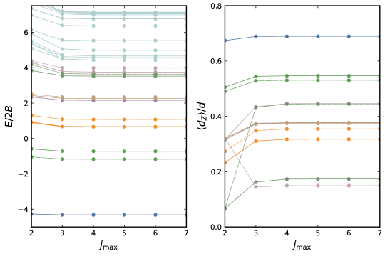
Figure 11: Low-energy spectrum and average dipole moment projections $\expectationvalue{d_{Z}}$ for linear molecules as a function of the angular momentum cutoff $j_{\mathrm{max}}$. We consider a distance $r=r_{B}$ and an external field $\mathcal{E}=4.0\bm{e}_{Z}$. Lines with the same colour and line type in the left and right panels indicate the same eigenstate.

For the low part of the spectrum examined in this work, the figure shows that the results quickly converge for $j_{\mathrm{max}}\gtrsim 4$, even though the dipole projection seems to be more sensitive to $j_{\mathrm{max}}$ than the energies. Because the dipole-dipole interaction and weak external fields only couple Fock states with small differences in $j$, a cutoff of $j_{\mathrm{max}}=4$ already captures the relevant contributions for the states with $\bar{j}\lesssim 2$ examined in this work. In addition, the figure shows clearly that the quality of the results decreases for small $j_{\mathrm{max}}$ and for higher excited states (see for example the light cyan lines in the spectrum). Naturally, to access higher parts of the energy spectrum it is necessary to consider bases with a higher cutoff.

Appendix D Asymmetric molecules

To examine how the eigenstates of two asymmetric top molecules depend on the values of the rotational constants, in figure 12 we show the energy spectrum at a fixed rescaled distance $r/r_{B}$ and no external field $\mathcal{E}=0$ as a function of the asymmetry parameter Zare (1988)

$$\kappa=\frac{2B-A-C}{A-C}\,,$$ (34)

where $\kappa=-1$ in the limit of prolate symmetric tops and $\kappa=1$ in the limit of oblate symmetric tops. We fix the values of $A$ and $C$, and thus we change the value of $B$ with $\kappa$. The colour scheme employed only differentiates states with different $\bar{j}$, as the labelling system used in the main text cannot clearly connect the prolate and oblate limits Zare (1988).

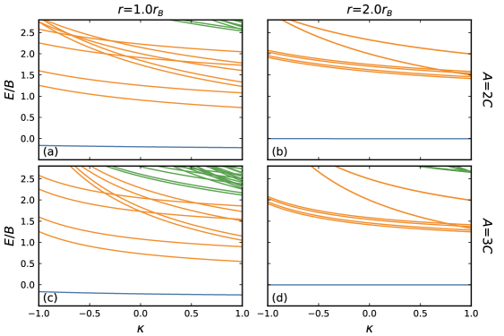
Figure 12: Low-energy spectrum for two asymmetric top molecules as a function of the asymmetry parameter $\kappa$. We consider a distance $r=r_{B}$ (left panels) and $r=2r_{B}$ (right panels), and no external electric field. We consider $A=2C$ (top panels) and $A=3C$ (bottom panels). Blue lines correspond to states with $\bar{j}=0$, orange lines correspond to states with $\bar{j}=1$, and green lines correspond to states with $\bar{j}=2$.

As stressed in the main text, the spectrum depends on both the rotational constants and the inter-molecular separation. For $r=2r_{B}$, the dipole-dipole interaction effect is weaker, and thus the spectrum as a function of $\kappa$ is similar to that of single asymmetric molecules (see Zare (1988)). On the other hand, for $r=r_{B}$ the molecules exhibit a rich spectrum. As discussed, measuring the spectrum of interacting molecules could be employed to extract the moments of inertia. We intend to explore these ideas further in future work.

References

References

- Carr et al. (2009) L. D. Carr, D. DeMille, R. V. Krems, and J. Ye, New Journal of Physics 11, 055049 (2009).
- Quéméner and Julienne (2012) G. Quéméner and P. S. Julienne, Chemical Reviews 112, 4949 (2012).
- Bohn et al. (2017) J. L. Bohn, A. M. Rey, and J. Ye, Science 357, 1002 (2017).
- Ni et al. (2008) K.-K. Ni, S. Ospelkaus, M. H. G. de Miranda, A. Pe’er, B. Neyenhuis, J. J. Zirbel, S. Kotochigova, P. S. Julienne, D. S. Jin, and J. Ye, Science 322, 231 (2008).
- Takekoshi et al. (2014) T. Takekoshi, L. Reichsöllner, A. Schindewolf, J. M. Hutson, C. R. Le Sueur, O. Dulieu, F. Ferlaino, R. Grimm, and H.-C. Nägerl, Physical Review Letters 113, 205301 (2014).
- Guo et al. (2016) M. Guo, B. Zhu, B. Lu, X. Ye, F. Wang, R. Vexiau, N. Bouloufa-Maafa, G. Quéméner, O. Dulieu, and D. Wang, Physical Review Letters 116, 205303 (2016).
- Park et al. (2015) J. W. Park, S. A. Will, and M. W. Zwierlein, Physical Review Letters 114, 205302 (2015).
- Molony et al. (2014) P. K. Molony, P. D. Gregory, Z. Ji, B. Lu, M. P. Köppinger, C. R. Le Sueur, C. L. Blackley, J. M. Hutson, and S. L. Cornish, Physical Review Letters 113, 255301 (2014).
- Tarbutt (2018) M. R. Tarbutt, Contemporary Physics 59, 356 (2018).
- McCarron (2018) D. McCarron, Journal of Physics B: Atomic, Molecular and Optical Physics 51, 212001 (2018).
- Norrgard et al. (2016) E. Norrgard, D. McCarron, M. Steinecker, M. Tarbutt, and D. DeMille, Physical Review Letters 116, 063004 (2016).
- Truppe et al. (2017) S. Truppe, H. J. Williams, M. Hambach, L. Caldwell, N. J. Fitch, E. A. Hinds, B. E. Sauer, and M. R. Tarbutt, Nature Physics 13, 1173 (2017).
- Anderegg et al. (2018) L. Anderegg, B. L. Augenbraun, Y. Bao, S. Burchesky, L. W. Cheuk, W. Ketterle, and J. M. Doyle, Nature Physics 14, 890 (2018).
- Ding et al. (2020) S. Ding, Y. Wu, I. A. Finneran, J. J. Burau, and J. Ye, Physical Review X 10, 021049 (2020).
- Kozyryev et al. (2017) I. Kozyryev, L. Baum, K. Matsuda, B. L. Augenbraun, L. Anderegg, A. P. Sedlack, and J. M. Doyle, Physical Review Letters 118, 173201 (2017).
- Augenbraun et al. (2020a) B. L. Augenbraun, Z. D. Lasner, A. Frenett, H. Sawaoka, C. Miller, T. C. Steimle, and J. M. Doyle, New Journal of Physics 22, 022003 (2020a).
- Vilas et al. (2022) N. B. Vilas, C. Hallas, L. Anderegg, P. Robichaud, A. Winnicki, D. Mitra, and J. M. Doyle, Nature 606, 70 (2022).
- Mitra et al. (2020) D. Mitra, N. B. Vilas, C. Hallas, L. Anderegg, B. L. Augenbraun, L. Baum, C. Miller, S. Raval, and J. M. Doyle, Science 369, 1366 (2020).
- Isaev and Berger (2016) T. A. Isaev and R. Berger, Physical Review Letters 116, 063006 (2016).
- Kozyryev et al. (2016) I. Kozyryev, L. Baum, K. Matsuda, and J. M. Doyle, ChemPhysChem 17, 3641 (2016).
- Augenbraun et al. (2020b) B. L. Augenbraun, J. M. Doyle, T. Zelevinsky, and I. Kozyryev, Physical Review X 10, 031022 (2020b).
- Isaev and Berger (2018) T. A. Isaev and R. Berger, CHIMIA 72, 375 (2018).
- Ivanov et al. (2020) M. V. Ivanov, F. H. Bangerter, P. Wójcik, and A. I. Krylov, The Journal of Physical Chemistry Letters 11, 6670 (2020).
- DeMille (2002) D. DeMille, Physical Review Letters 88, 067901 (2002).
- Yelin et al. (2006) S. F. Yelin, K. Kirby, and R. Côté, Physical Review A 74, 050301 (2006).
- Wei et al. (2011) Q. Wei, S. Kais, B. Friedrich, and D. Herschbach, The Journal of Chemical Physics 135, 154102 (2011).
- Herrera et al. (2014) F. Herrera, Y. Cao, S. Kais, and K. B. Whaley, New Journal of Physics 16, 075001 (2014).
- Hudson and Campbell (2018) E. R. Hudson and W. C. Campbell, Physical Review A 98, 040302 (2018).
- Ni et al. (2018) K.-K. Ni, T. Rosenband, and D. D. Grimes, Chemical Science 9, 6830 (2018).
- Yu et al. (2019) P. Yu, L. W. Cheuk, I. Kozyryev, and J. M. Doyle, New Journal of Physics 21, 093049 (2019).
- Gregory et al. (2021) P. D. Gregory, J. A. Blackmore, S. L. Bromley, J. M. Hutson, and S. L. Cornish, Nature Physics 17, 1149 (2021).
- Baron et al. (2014) J. Baron, W. C. Campbell, D. DeMille, J. M. Doyle, G. Gabrielse, Y. V. Gurevich, P. W. Hess, N. R. Hutzler, E. Kirilov, I. Kozyryev, B. R. O’Leary, C. D. Panda, M. F. Parsons, E. S. Petrik, B. Spaun, A. C. Vutha, and A. D. West, Science 343, 269 (2014).
- Lim et al. (2018) J. Lim, J. Almond, M. Trigatzis, J. Devlin, N. Fitch, B. Sauer, M. Tarbutt, and E. Hinds, Physical Review Letters 120, 123201 (2018).
- Hutzler (2020) N. R. Hutzler, Quantum Science and Technology 5, 044011 (2020).
- Mitra et al. (2022) D. Mitra, K. H. Leung, and T. Zelevinsky, Physical Review A 105, 040101 (2022).
- Krems (2019) R. V. Krems, Molecules in electromagnetic fields: from ultracold physics to controlled chemistry, 1st ed. (John Wiley & Sons, Hoboken, NJ, 2019).
- Ni et al. (2010) K.-K. Ni, S. Ospelkaus, D. Wang, G. Quéméner, B. Neyenhuis, M. H. G. de Miranda, J. L. Bohn, J. Ye, and D. S. Jin, Nature 464, 1324 (2010).
- Lahaye et al. (2009) T. Lahaye, C. Menotti, L. Santos, M. Lewenstein, and T. Pfau, Reports on Progress in Physics 72, 126401 (2009).
- Baranov et al. (2012) M. A. Baranov, M. Dalmonte, G. Pupillo, and P. Zoller, Chemical Reviews 112, 5012 (2012).
- Kovrizhin et al. (2005) D. L. Kovrizhin, G. V. Pai, and S. Sinha, Europhysics Letters (EPL) 72, 162 (2005).
- De Marco et al. (2019) L. De Marco, G. Valtolina, K. Matsuda, W. G. Tobias, J. P. Covey, and J. Ye, Science 363, 853 (2019).
- Valtolina et al. (2020) G. Valtolina, K. Matsuda, W. G. Tobias, J.-R. Li, L. De Marco, and J. Ye, Nature 588, 239 (2020).
- Moses et al. (2017) S. Moses, J. Covey, M. Miecnikowski, D. Jin, and J. Ye, Nature Physics 13, 13 (2017).
- Di Lauro (2020) C. Di Lauro, Rotational structure in molecular infrared spectra, second edition ed. (Elsevier, Amsterdam, Netherlands ; Cambridge, MA, 2020).
- Koch et al. (2019) C. P. Koch, M. Lemeshko, and D. Sugny, Reviews of Modern Physics 91, 035005 (2019).
- Tutunnikov et al. (2018) I. Tutunnikov, E. Gershnabel, S. Gold, and I. S. Averbukh, The Journal of Physical Chemistry Letters 9, 1105 (2018).
- Micheli et al. (2007) A. Micheli, G. Pupillo, H. P. Büchler, and P. Zoller, Physical Review A 76, 043604 (2007).
- Górecki and Rzążewski (2017) W. Górecki and K. Rzążewski, EPL (Europhysics Letters) 118, 66002 (2017).
- Dawid et al. (2018) A. Dawid, M. Lewenstein, and M. Tomza, Physical Review A 97, 063618 (2018).
- Dawid and Tomza (2020) A. Dawid and M. Tomza, Physical Chemistry Chemical Physics 22, 28140 (2020).
- Sroczyńska et al. (2022) M. Sroczyńska, A. Dawid, M. Tomza, Z. Idziaszek, T. Calarco, and K. Jachymski, New Journal of Physics 24, 015001 (2022).
- Wall and Carr (2009) M. L. Wall and L. D. Carr, New Journal of Physics 11, 055027 (2009).
- Gorshkov et al. (2011) A. V. Gorshkov, S. R. Manmana, G. Chen, J. Ye, E. Demler, M. D. Lukin, and A. M. Rey, Physical Review Letters 107, 115301 (2011).
- Wall et al. (2013) M. L. Wall, K. Maeda, and L. D. Carr, Annalen der Physik 525, 845 (2013).
- Wall et al. (2015) M. L. Wall, K. Maeda, and L. D. Carr, New Journal of Physics 17, 025001 (2015).
- Zare (1988) R. N. Zare, Angular momentum: understanding spatial aspects in chemistry and physics (Wiley, New York, 1988).
- Man (2013) P. P. Man, Concepts in Magnetic Resonance Part A 42, 197 (2013).
- Strebel et al. (2010) M. Strebel, F. Stienkemeier, and M. Mudrich, Physical Review A 81, 033409 (2010).
- Patterson and Doyle (2012) D. Patterson and J. M. Doyle, Molecular Physics 110, 1757 (2012).
- Schoolery and Sharbaugh (1951) J. N. Schoolery and A. H. Sharbaugh, Physical Review 82, 95 (1951).
- Meerts and Ozier (1981) W. L. Meerts and I. Ozier, The Journal of Chemical Physics 75, 596 (1981).
- Lovas et al. (2009) F. Lovas, D. Plusquellic, B. H. Pate, J. L. Neill, M. T. Muckle, and A. J. Remijan, Journal of Molecular Spectroscopy 257, 82 (2009).
- Doçaj et al. (2016) A. Doçaj, M. L. Wall, R. Mukherjee, and K. R. Hazzard, Physical Review Letters 116, 135301 (2016).
- Wall et al. (2017) M. L. Wall, N. P. Mehta, R. Mukherjee, S. S. Alam, and K. R. A. Hazzard, Physical Review A 95, 043635 (2017).
- Isaule et al. (2022) F. Isaule, R. Bennett, and J. B. Götte, Physical Review A 106, 013321 (2022).