Estimating the parameters of epidemic spread on multilayer random graphs:
a classical and a neural network approach

Abstract

In this paper, we study the spread of a classical SIR process on a two-layer random network, where the first layer represents the households, while the second layer models the contacts outside the households by a random scale-free graph. We build a three-parameter graph, called polynomial model, where the new vertices are connected to the existing ones either uniformly, or preferentially, or by forming random triangles. We examine the effect of the graph’s properties on the goodness of the estimation of the infection rate $\tau$.

In the classical approach, to estimate $\tau$ one needs to approximate the number of SI edges between households, since the graph itself is supposed to be unobservable. Our simulation study reveals that the estimation is poorer at the beginning of the epidemic, for larger preferential attachment parameter of the graph, and for larger $\tau$. We can improve the estimate either by (i) adjusting it by a graph-dependent factor at a fixed time in the earlier phase of the epidemic, or (ii) by applying a shift in the estimation of the SI edges. Furthermore, we establish our method to be robust to changes in average clustering of the graph model.

We also extend a graph neural network (GNN) approach for estimating contagion dynamics for our two-layered graphs. We find that dense networks offer better training datasets. Moreover, GNN perfomance is measured better using the $l_{2}$ loss function rather than cross-entropy.

1 Introduction

Modelling epidemic spread has been an actively studied field in the last decades, and especially in the last three years, due to the outbreak of the SARS-CoV-2 pandemic. There are several approaches to model and predict epidemics, such as differential equations, or agent-based models. In the current work we are interested in a question coming from the application of random graphs for modelling epidemic spread. Within this area, a very general question is the following: how does the structure of the graph affect the behaviour of the epidemic process, and how does this change the goodness of the estimates of the parameters? Of course, the answer often depends on the methods that we use [8, 12].

When we use random graphs for modelling epidemic spread, it is quite common to use multilayer models, where different layers represent different types of communities [2, 7, 8, 16]. In particular, in the household model introduced and analysed by Ball [3, 4], we can start with a layer for households: this consists of disjoint, small complete graphs. Then we can add a layer representing the connections between households, which can be either a complete graph, as in the original household model, or a random graph with a more inhomogeneous structure, closer to real-world networks. In such models there are many interesting questions about parameter sensitivity, the effect of the structure of the graph on the epidemic process, or about estimating the parameters, already in the two-layer case; see e.g. [8] for a recent survey on this topic. Although there are some partial results, in general, we can say that there are still various open questions in this area, for example:

1. How can we estimate the infection parameters if the second layer is a random graph of a more complex structure, e.g. a preferential attachment graph, or a random graph with duplications?

2. How does the presence of smaller or larger clusters affect the methods of parameter estimation? For example, the second (or other additional layers) can also consist of smaller complete graphs, representing the workplaces or school classes where a group of people meet each other regularly [2], and the general methods for the complete graph, which is homogeneous, might not work in this case.

3. What is the necessary information from the network that is needed for parameter estimation? In real-world problems, very often we do not know the graph exactly, only some basic statistics can be determined by sampling (e.g. the density of edges, or the density of triangles). For example, [19] shows a method using deep learning methods to reconstruct the precise structure of the graph from a smaller sample; but this also shows that we cannot assume that we have a full description of the network.

When we examine these questions, there are several, essentially different approaches to estimate the parameters. For example, [11] compares maximum likelihood estimates with Bayesian estimates in case of a complete graph (without household structure). The papers [7, 14, 17] also present Bayesian inference for similar problems about epidemic spread. On the other hand, the methods based on neural networks are also promising for these questions, see e.g. the recent results in [15].

In the current project we examined the effect of the preferential attachment structure and the clustering coefficient (number of triangles) on the goodness of the estimation of the infection rate in household models, and compared classical (maximum likelihood) and neural network methods from this point of view. The question about the clustering coefficient is already mentioned in Section 6.2 of [8]. Since this seems to be an open problem already in the two-layer case, we consider only the household layer and an additional random graph, which is in most cases a preferential attachment graph with tunable clustering coefficient (see e.g.  [10] or [18] for such models).

2 The model: SIR process on a household graph with tunable clustering coefficient

In the sequel, we focus on two-layer random graphs, where the first layer, the graph of households is deterministic, but the second layer, the connections between the households are chosen randomly. In addition, for simplicity, we keep the size of the households fixed.

An important point in our studies will be the clustering coefficient of the second layer. Loosely speaking, we are interested in the effect of a larger probability that the neighbors of a given vertex are connected to each other. Before we define the model, we formulate the versions of the clustering coefficient which we will use.

Definition 1

Let $G=(V,E)$ be a simple graph.
The global clustering coefficient is the ratio of three times the number of triangles to the number of pairs of djacent edges in $G$.
The average local clustering coefficient $C(G)$ is defined as follows: for each vertex $v$, let $T_{G}(v)$ be the number of triangles containing $v$, and $C_{G}(v)$ the number of paths of length $2$ with the middle point $v$; that is, $\binom{N_{G}(v)}{2}$, where $N_{G}(v)$ is the number of neighbors of $v$. Then

$$C(G)=\frac{1}{|V|}\sum_{v\in V}\frac{T_{G}(v)}{C_{G}(v)}.$$

To put it in another way, for each vertex $v$, we calculate the probability that two uniformly randomly chosen neighbors of $v$are connected to each other with an edge, and average out this probability for all vertices of the graph $G$.

When modelling real-world networks, preferential attachment models are often used, at least as approximative models. Within this family, our goal was to choose graphs whose clustering coefficient is close to the typical clustering coefficient of real-world networks, which is often not very close to zero. From our point of view, the original Barabási–Albert graph [5] is not a very good choice, due to the result of Bollobás and Riordan [6, Theorem 12], proving that the global clustering coefficient of a Barabási–Albert graph on $n$ vertices is asymptotically equal to $c(\log n)^{2}/n$, which goes to $0$ as $n$ tends to infinity. On the other hand, since epidemic spread is based on local dynamics, instead of the global clustering coefficient, we also are also interested in the realistic choice of the average local clustering coefficient. As for the original preferential attachment models, the average local clustering coefficient for vertices of degree $d$ was analyzed in [13].

Hence, to study models with realistic clustering coefficients, instead of the Barabási–Albert graph, we used the polynomial graph models defined by Ostroumova, Ryabchenko and Samosvat [18]. In particular, we study the three-parameter model described in Section 5.1 of the above paper, or its minor modifications. We start with an arbitrary graph with $n_{0}$ vertices and $mn_{0}$ directed edges. Then, in this growing graph process, in the $(n+1)$st step, we add a new vertex labelled $(n+1)$ to the graph, together with $m$ directed edges. The edges are directed from the new vertex $(n+1)$ towards another vertex from the set $\{1,\ldots,n+1\}$ (thus loops are also allowed). We denote the graph after $n$ steps by $G_{n}$. In this particular model we choose an even number $m=2p$, and the $m$ edges are chosen in $p$ pairs, where the choice of these $p$ pairs is independent and identically distributed. The choice of one pair of edges goes as follows (we give here the notations of [18] as well, but in the sequel we use our own notation):

• With probability $p_{\rm pa}=\alpha$, we choose two vertices independently from $\{1,\ldots,n\}$, with probability proportional to their in-degree (preferential attachment component), and connect a new edge to these vertices.

• With probability $p_{\rm u}=\delta$, we choose two vertices independently from $\{1,\ldots,n+1\}$, with equal probability (uniform component), and connect a new edge to these vertices.

• With probability $p_{\rm tr}=\beta$, we choose a random edge of $G_{n}$ uniformly, and connect a new edge to both of its endpoints.

Naturally, we have $p_{\rm pa}+p_{\rm tr}+p_{\rm u}=1$. The authors of [18] also show that if $2p_{\rm pa}+p_{\rm tr}<1$, then the global clustering coefficient of the graph does not tend to zero as $n\to\infty$, but is asymptotically

$$\frac{3(1-2p_{\rm pa}-p_{\rm tr})p_{\rm tr}}{5m-1-2(2m-1)(2p_{\rm pa}+p_{\rm tr})}.$$

In addition, the asymptotic degree distribution is scale-free with exponent $\gamma=1+\frac{2}{2p_{\rm pa}+p_{\rm tr}}$. It seems that there is no closed formula for the limit of the local average clustering coefficient in this model, but computer simulations show that we can tune this quantity nicely (this is presented in [18], and in the next section we also analyze this in more details).

We use the following minor modification of the algorithm, which also works when $m=2p+1$ is odd: first we randomize the number of triangles, which has a binomial distribution of order $p$ with parameter $p_{\rm tr}$, and the remaining edges are formed one-by-one according to preferential attachment (with probability $p_{\rm pa}/(p_{\rm pa}+p_{\rm u})$) or uniform attachment (with probability $p_{\rm u}/(p_{\rm pa}+p_{\rm u})$). Also, we exclude loop-edges. Multiple edges are allowed, but when calculating the clustering coefficient, we take the multiplicity of each edge as $1$.

Putting this together with the household model, we obtain the following model of epidemic spread on a two-layer random graph:

1. We have $N$ vertices, who live in households of size $N_{hh}$. Usually we will use $N_{hh}=5$. Each household is a complete graph with edges of weight $1$. Of course, this is is not a realistic choice for households, but these can represent other small group of people who regularly meet e.g. at workplaces or school.

2. Independently of the household layer, we add a polynomial graph model on the $N$ vertices, defined above. (This can be done for example by first forming the polynomial graph, then grouping the vertices into random households of size $N_{hh}$.) This represents the connections between households. The weight of these edges will be fixed, $w$, which is considered as a given constant and can be used in the estimations (in the simulations we will typically use $w=0.4$).

3. We run an SIR (susceptible-infected-recovered) process on this random graph. The infection rate within households is $\tau$, while the infection rate on each edge connecting individuals from different households is $\tau\cdot w$. Our goal is to estimate the infection rate $\tau$ given the number of S, I, R vertices and maybe some additional information.

An alternative for the polynomial model can be the model of Holme and Kim [10]. For this model, which also has a preferential attachment component, it is proved that the global clustering coefficient tends to zero as the number of vertices tends to infinity, but the average local clustering coefficient has a positive limit.

3 Parameter sensitivity

In this section we study the effect of the different parameters on the epidemic curve in the model defined in Section 2. Based on real data, the average local clustering coefficient of a typical online social network is between $0.1$ and $0.4$ [21]. We may assume that this value is not significantly different for online networks and real-world social networks, through which contagious diseases spread.

We studied the average local clustering coefficients of graphs with $N=5000$ vertices, generated from the 3-parameter polynomial random graph model. Throughout, we used a random initial configuration of size $N_{0}=50$. For the results shown in Figure 1, we chose $m=4$, and changed the values of $p_{\rm pa}$ and $p_{\rm tr}$ using an equispaced grid, with $p_{\rm pa}+p_{\rm tr}\leq 1$. For each choice of the parameters, we calculated the average local clustering coefficient of the polynomial graph (left panel), as well as that of the two-layer household graph (right panel), with household size $5$. Each clustering coefficient in the figure is the mean of $10$ simulations. From the figure, we can see that the average local clustering coefficient of the polynomial graph ranges from almost $0$ to around $0.27$. The strongest clustering occurs when the triangle component takes its maximal value $1$. We can see that the average local clustering coefficient depends on both the triangle and the preferential component in a monotonic increasing way, and of the two, the triangle component has a stronger effect. The reason for this is that in the polynomial graph, as the new vertex is connected to old vertices, there is a small chance to obtain any triangles, unless the triangle component is high.

When we add the layer of households, i.e. small complete graphs, the clustering coefficient naturally increases: it ranges between $0.12$ and $0.33$. Observe that the average local clustering coefficient still depends on both the triangle and the preferential component in a monotonic increasing way. However, interestingly, now the preferential attachment component has a stronger effect – at least when the uniform component is very small – the highest clustering occurs when $p_{\rm pa}$ takes its maximal value $1$. An explanation for this could be the following. When we have a purely preferential graph, vertices with very high degree (so-called hubs) emerge. When we form the households, the neighbors of hubs get connected with each other, thus forming many triangles.

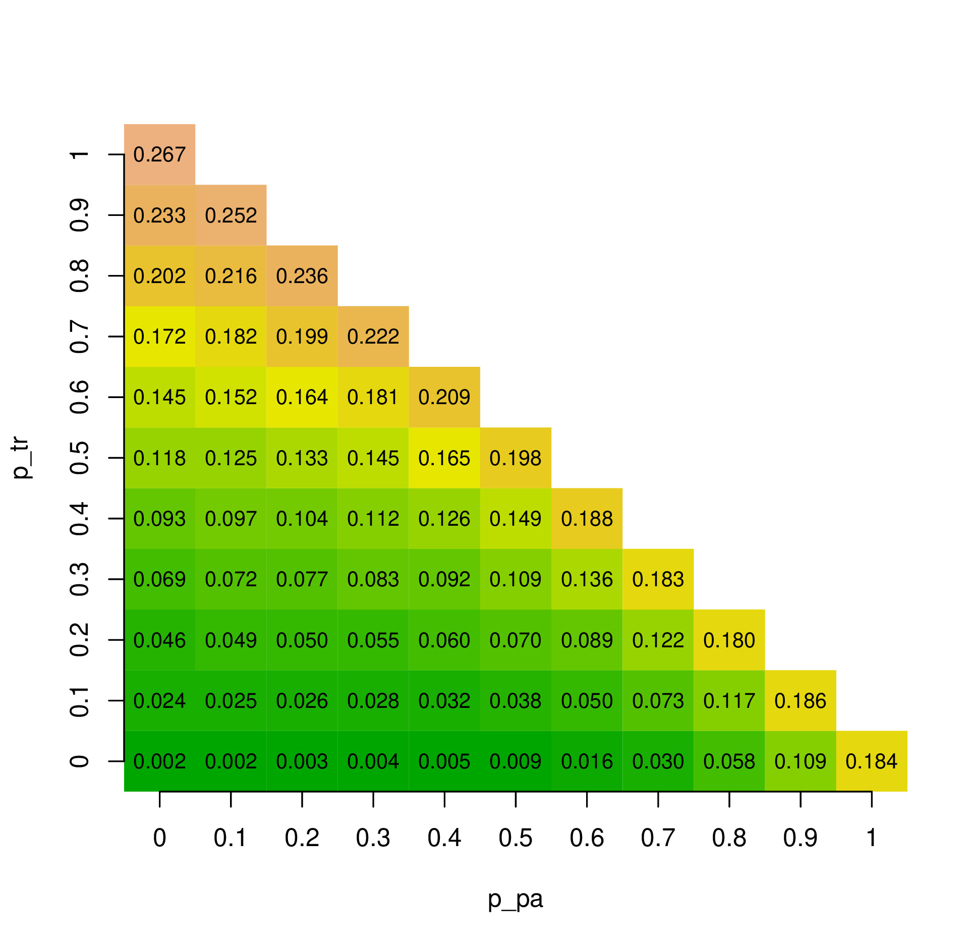
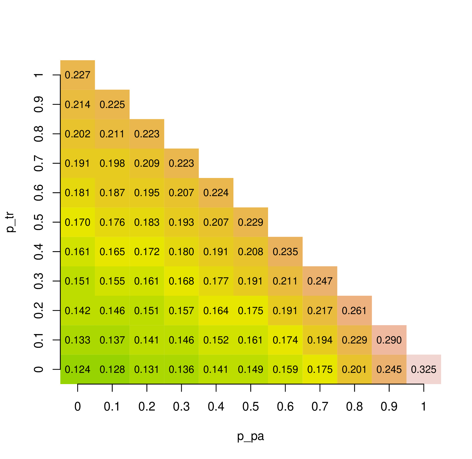
Figure 1: Average local clustering coefficient for the polynomial graph (left) and the two-layer graph (right). The rows show the value of $p_{\rm tr}$, the columns show the values of $p_{\rm pa}$. $N=5000$, $m=4$.

3.1 Choice of the infection rates

In the following sections we will compare epidemic spread on the two-layer graph with different values of $p_{\rm pa}$ and $p_{\rm tr}$. Of course, if we are interested in the effect of the structure of the graph, we have to keep the infection rate $\tau$ fixed. In order to choose realistic values of $\tau$, we now calculate the value of $R_{0}$, the basic reproduction number (the expected number of infections caused by an infected individual at the beginning of the epidemic. It is well known that the epidemic spreads only if $R_{0}\geq 1$. For example, in one of the most intense periods of the coronavirus pandemic, in Spring 2020 in Italy, $R_{0}$ is estimated to be between $2.43$ and $3.1$ [9]. Hence we will choose $\tau$ such that $R_{0}$ is between $1$ and $3$.

Now let us see how $R_{0}$ depends on $\tau$. The infection rate within households is $\tau$, while the infection rate between households is $w\cdot\tau$. The degree of a vertex within its household is $N_{\rm hh}-1=4$, while the average degree of a vertex between households is approximately $2m$ (we omit the effect of the initial configuration, and later on, at each step, one new vertex is added with $m$ new edges).

Let us assume that vertex $v$ gets infected, and calculate $R_{0}$, the expected number of infections it causes. From [20] (see Proposition $2.2$) we know that the value of $R_{0}$ is $(d-1)\cdot\frac{\tau}{\tau+\gamma}$ for a random $d$-regular graph (where $\tau$ is the infection rate and $\gamma$ is the recovery rate), where the subtraction corresponds to the individual that infected $v$. In our model, each vertex has $N_{hh}-1$ edges with weight $1$ within households, and, on average, $2m$ edges with weight $w$ between households. Hence, by simplifying the calculations, the probability that $v$ was infected by some of its household members is $(N_{\rm hh}-1)/(N_{\rm hh}-1+w\cdot 2m)$. Hence, similarly to the value of $R_{0}$ in the configuration model (but taking into consideration that the infection rate between households is $w\cdot\tau$), we obtain that

$$R_{0} \approx\frac{N_{\rm hh}-1}{N_{\rm hh}-1+w\cdot 2m}\cdot\bigg{(}\frac{(N_{\rm hh}-2)\cdot\tau}{\tau+\gamma}+\frac{2m\cdot w\cdot\tau}{w\cdot\tau+\gamma}\bigg{)}$$

$$\quad+\frac{w\cdot 2m}{N_{\rm hh}-1+w\cdot 2m}\cdot\bigg{(}\frac{(N_{\rm hh}-1)\cdot\tau}{\tau+\gamma}+\frac{(2m-1)\cdot w\cdot\tau}{w\cdot\tau+\gamma}\bigg{)}$$

By using this formula with $N_{\rm hh}=5$, $m=4$, $w=0.4$ and recovery rate $\gamma=1$, for $\tau=0.3$ we get $R_{0}\approx 1.6$, while for $\tau=0.6$, we get $R_{0}\approx 2.75$. These values are in the supercritical case, and might be realistic for the coronavirus pandemic in the intensive phases, so we will use these infection rates for our studies for parameter sensitivity.

3.2 Effect of the preferential attachment component

When we study the spread of the epidemic with different parameters of the polynomial model, first we are interested in the effect of the preferential attachment component on the proportion of infected vertices, and on the number of SI edges between households. The first layer, the household graph is fixed, with households of size $N_{\rm hh}=5$. As for the second layer, in the polynomial model (defined in Section 2), we fix the weight of the triangle component ($p_{tr}=0.1$), and increase the weight of the preferential attachment component: $p_{\rm pa}=0.1,0.2,0.3,0.4,0.5$. The number of vertices is $5000$, and for each set of parameters, we generate five graphs from the polynomial model, with $m=3$. Then the SIR process is repeated five times on each graph (the infection rate was $\tau=0.3$, while the recovery rate was $\gamma=1$), hence each curve is the average of $25$ simulations. The set of infected individuals in the beginning is a randomly chosen $5\%$ of the whole population (chosen independently for each simulation).

Figure 2 shows the results of the simulations. We can see that the preferential attachment component has a significant effect on the process (at least if the weight of the preferential attachment component is at least $0.4$): the larger the preferential attachment component is, the larger the peak of the epidemics is. As we can also see from Figure 1, the estimated average local clustering coefficient of the two-layer graph ranges from $0.14$ (for $p_{pa}=0.1$) to $0.16$ (for $p_{pa}=0.5$) for this set of parameters for the two-layer graph. For the polynomial graph itself, the local clustering coefficient goes from $0.026$ to $0.044$. Since the differences are not that large, in this case what we can see is mostly the effect of the preferential attachment structure: if the preferential attachment component has a higher weight, then we have more vertices with a very large degree, who can spread the infection to many vertices very quickly.

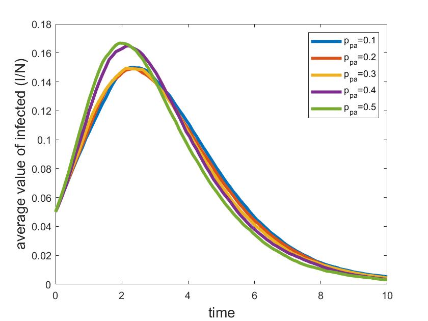
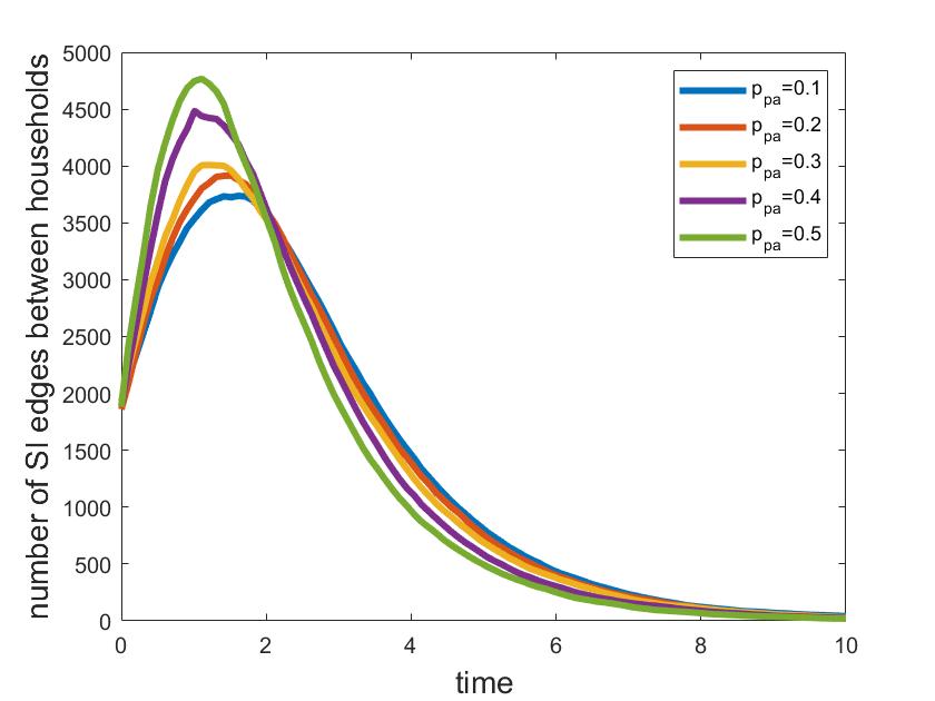
Figure 2: Proportion of infected vertices (left) and number of SI edges (right) with $p_{tr}=0.1$ fixed, $N=5000$ vertices, $m=4$, $\tau=0.3$. Each curve is the average of $25$ simulations

We repeated the same simulations in the case when $\tau=0.6$ (this corresponded to a basic reproduction number larger than $2$). Figure 3 shows the results. In this case the effect of the preferential attachment component seems to be less significant, but still we can see mononiticity with respect to this parameter in the behavior of the number of $SI$ edges between the households.

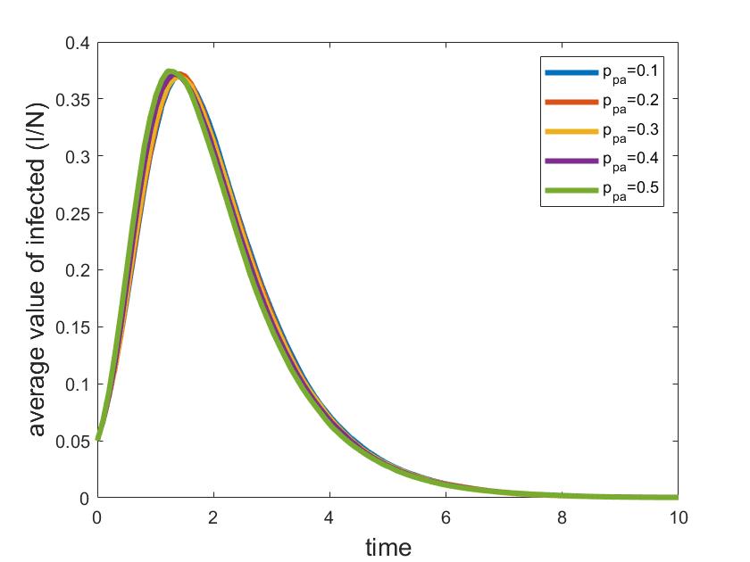
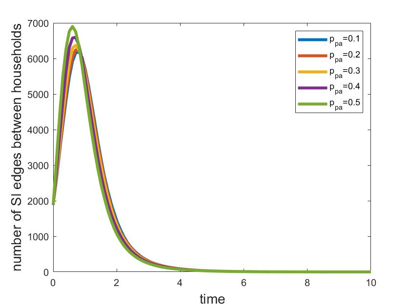
Figure 3: Proportion of infected vertices (left) and number of SI edges (right) with $p_{tr}=0.1$ fixed, $N=5000$ vertices, $m=4$, $\tau=0.6$. Each curve is the average of $25$ simulations

3.3 Effect of the triangles

Now we are interested in the effect of the weight of the triangle component. The simulations are very similar to the ones in the previous subsection, but now we keep $p_{\rm pa}=0.2$ fixed, and we change $p_{\rm tr}$ from $0$ to $0.4$. In this case the estimated average local clustering coefficient goes from $0.133$ to $0.174$ (according to Figure 1), so the differences are somewhat larger than in the previous case. Figure 4 shows the results of the simulations. Here the effect is less significant, compared to 2, although the difference in the clustering coeffient was larger. Monotonicity is not clear from the figure. Heuristically, we would expect that the larger value of an average local clustering coefficient (larger $p_{\rm tr}$) leads to a smaller peak, as the neighbors of an infected vertex might already be infected by their common neighbors of this infected vertex. However, this effect is not visible on the figure. Altogether, these results suggest that the preferential attachment component has a stronger effect on the height of the peak and on the spread of the epidemic.

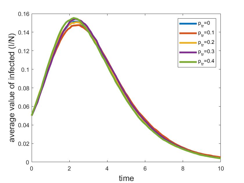
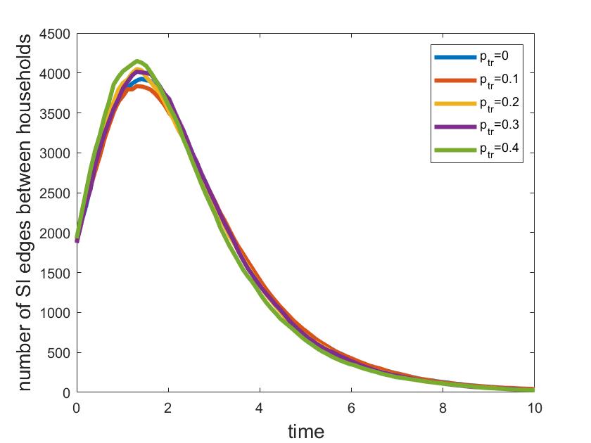
Figure 4: Proportion of infected vertices (left) and number of SI edges (right) with $p_{pa}=0.2$ fixed, $5000$ vertices, $m=4$, $\tau=0.3$. Each curve is the average of $25$ simulations

4 Parameter estimation based on the maximum likelihood method

Our starting point is the argument of [11], where the maximum likelihood estimation for the recovery and infection rates is determined in the case of the complete graph. If we notice that the estimate depends only on local properties (the number of infections and the number of SI edges), we can see that there is a good chance that this can work for our more complex graph as well.

In [11], the authors derive the following maximum likelihood estimates in the case of the complete graph for the recovery rate $\gamma$ and the infection rate $\tau$ (which is the same for all pairs of vertices in the case of the complete graph).

The estimate of the recovery rate:

$$\gamma=\frac{z_{R}}{\int_{0}^{\overline{T}}I_{t}dt}=\frac{z_{R}}{\sum_{t_{i}\leq\overline{T}}I_{t_{i}}\cdot(t_{i}-t_{i-1})},$$

where

• $z_{R}$ is the total number of events when a vertex recovers, that is, the number of recovered vertices at $\overline{T}$;

• $S_{t},I_{t},R_{t}$ denotes the number of vertices in the states $S,I,R$ at time $t$;

• $0<t_{1}<t_{2}<\ldots<t_{i}$ are the time points where there is an infection or a recovery;

• $\overline{T}$ is an appropriately chosen time (typically $5/6$ times the time until the epidemic process stops).

The estimate of the infection rate:

$$\hat{\tau}=\frac{z_{I}}{\int_{0}^{T}E_{t}^{SI}\,dt}=\frac{z_{I}}{\sum_{t_{i}<T}E_{t_{i}}^{SI}(t_{i}-t_{i-1})},$$

where

• $z_{I}$ is the total number of events when a vertex gets infected;

• $E_{t}^{SI}$ is the number of SI edges (edges with one susceptible and one infected endpoint).

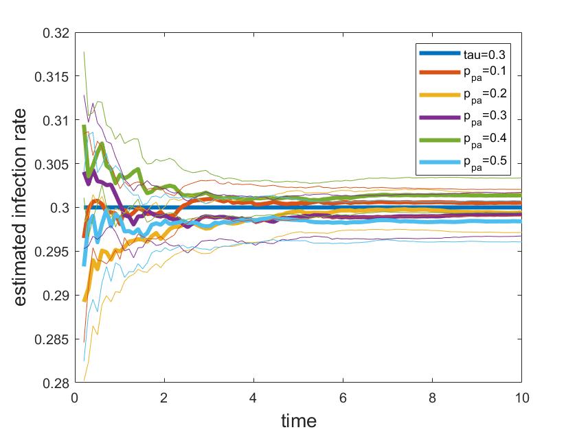
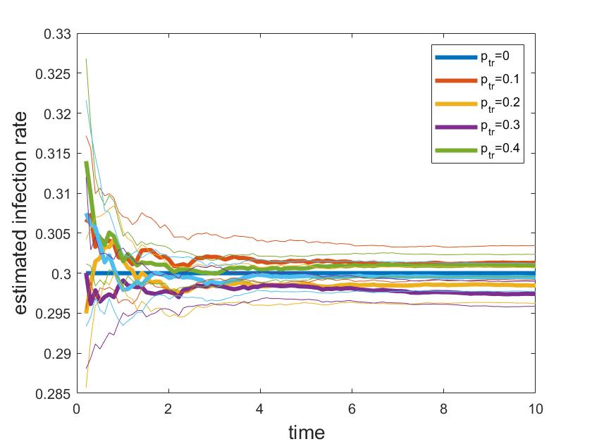
Figure 5: Estimate of the infection parameter $\tau$ for different polynomial random graphs if the number of $SI$ edges is known exactly. The graph has $N=5000$ vertices, $m=4$, $\tau=0.3$, $\gamma=1$, we randomize five graphs for each parameter setup, and run five SIR simulations on each graph; the thick curve is the mean of 25 trajectories, thin curves correspond to the $95\%$ confidence intervals based on the 25 simulations. Left: $p_{\rm tr}=0.1$ is fixed; right: $p_{\rm pa}=0.2$ is fixed.

So far, this formula does not use much from the structure of the graph, so we expect that this works nicely for other graphs as well, after the appropriate modifications:

$$\hat{\tau}=\frac{z_{I}}{\int_{0}^{T}W_{t}^{SI}\,dt}=\frac{z_{I}}{\sum_{t_{i}<T}W_{t_{i}}^{SI}(t_{i}-t_{i-1})},$$ (1)

where

• $z_{I}$ is the total number of events when a vertex gets infected;

• $W_{t}^{SI}$ is the total weight of SI edges, including the edges within households with weight $1$ and the edges between households with weight $w$.

Indeed, as we can see on Figure 5, the estimated infection rate converges quickly to the real value of $\tau$ even in our case, in the polynomial model, independently of the parameters of the graph model.

However, this formula heavily relies on the number of SI edges, which might not be easy to measure during an epidemic. In an earlier (unpublished) work [1], the following formula was used to estimate the number of SI edges going between the households, in the case when the graph connecting the households is an Erdős–Rényi graph (which has a much more homogeneous structure than the preferential attachment graph):

$$\hat{E}^{SI,o}_{t}=I_{t}\cdot\bigg{(}d-\frac{wd}{wd+N_{\rm hh}-1}\bigg{)}\cdot\frac{S_{t}}{N},$$

where $d$ is the average number of the neighbors of a vertex outside its household, and $w$ is the weight of the edges going between different households (both were considered as fixed, known quantities). The idea is that each infected vertex has $d$ edges outside its household, each is susceptible with probability $S_{t}/N$, but with a certain probability, the vertex was infected by one of its neighbors outside the household, and in this case the number of neighbors that we take into account is $d-1$. Once we have this estimate, the estimate of $W_{t}^{SI}$ is simply the number of the $SI$ edges within household plus $w$ times the $\hat{E}^{SI,o}_{t}$, and we can use equation (1) to get the estimate of $\tau$.

Although the degree distribution of the polynomial model is very different from that of the Erdős–Rényi graph (due to the preferential attachment dynamics), and the larger clustering coefficient might have an effect of the estimates as well, this formula was our starting point for the estimate of the infection rate $\tau$ for the polynomial model. Similarly to [1], we assumed that the number of SI edges within households is known (this would be the case if people went to tests together with their household members, or at least we could sample households and test everyone at the same time).

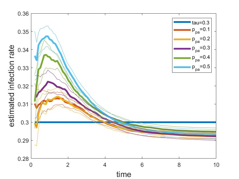
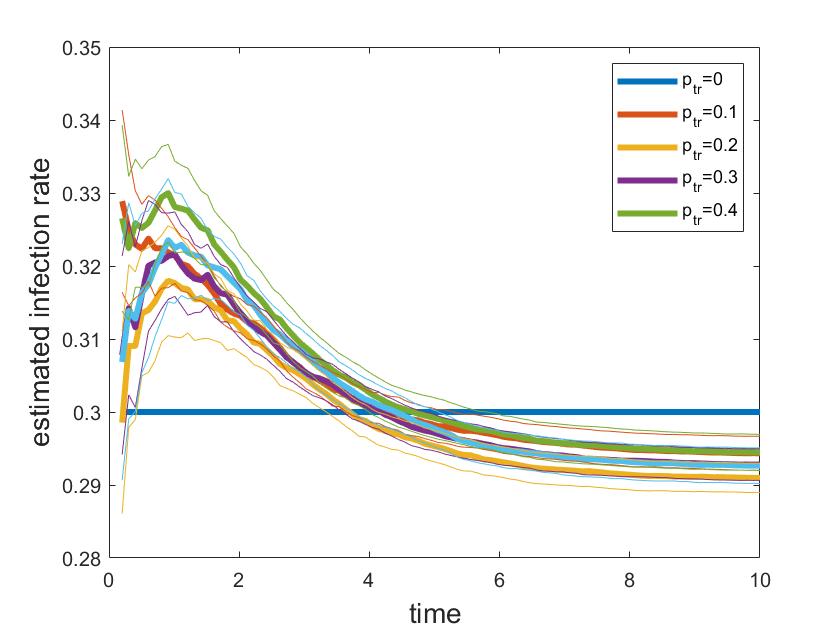
Figure 6: Estimate of the infection parameter $\tau$ for different polynomial random graphs if the number of $SI$ edges between households is not known. The graph has $N=5000$ vertices, $m=4$, $\tau=0.3$, $\gamma=1$, we randomize five graphs for each parameter setup, and run five SIR simulations; the thick curve is the mean of 25 trajectories, thin curves correspond to the $95\%$ confidence intervals based on the 25 simulations. Left: $p_{\rm tr}=0.1$ is fixed; right: $p_{\rm pa}=0.2$ is fixed.

On Figure 6 we can see how the formula with the estimated number of $SI$ edges works as we proceed in time, for different parameter setups. The simulation was run on graphs of $5000$ vertices, with the polynomial model with $m=4$, with $\tau=0.3$ fixed (recall that $R_{0}$ is approximately $1.6$ with this parameter setup). Each thick curve is the average of $25$ curves, corresponding to 5 graphs for each $p_{\rm pa}$ (left) and $p_{\rm tr}$ (right) and 5 SIR simulations on each graph. The thin curves represent the $95\%$ confidence intervals based on these $25$ runs. On the horizontal axis, time is measured in units (the recovery rate $\gamma=1$ is fixed). Recall from Figure 2 that, with the same parameter setup, the peak of the epidemic is around 2. At this time, in the case when we change $p_{\rm pa}$ (left figure), the estimate is between $0.31$ and $0.35$, which is significantly worse than in the case where the total number of SI edges are known (Figure 5). We can also see that the estimate is a monotone function of the weight of the preferential attachment component: the higher the weight of the preferential component is, the higher the error of the estimate is, at least in the first part of the epidemic. Hence it is worth looking for estimates that improve (1) by using the degree distribution or other structural properties of the graph that are closely related to the preferential attachment dynamics. On the right-hand side figure, where the weight of the preferential attachment component is fixed and the weight of the triangle component is changing, the convergence is much faster, and it does not seem to depend on the parameters, at least we cannot see any monotonicity. This corresponds to the fact that in this case the spread of the epidemic was also almost the same for the different values or $p_{\rm tr}$ (recall Figure 4). We can conclude that the degree distribution has a stronger effect on the estimates than the clustering coefficient (which is between $0.14$ and $0.16$ on the left-hand side, but changes from $0.13$ to $0.17$ on the right-hand side, according to Figure 1).

Figure 7 shows the estimate of $\tau$ at a time which is close to the end of the epidemic: this estimates uses the trajectory until the point when $5/6$ of the total epidemic events (infection or recovery) have already occured. We can see that the estimate works quite well for different values of $\tau$, independently of the parameters of the graph, but the estimate is getting worse if we increase the value of the infection parameter. This also suggests that it is worth using more elaborate methods for the estimates.

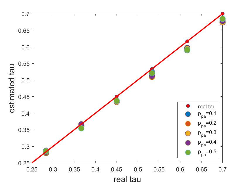
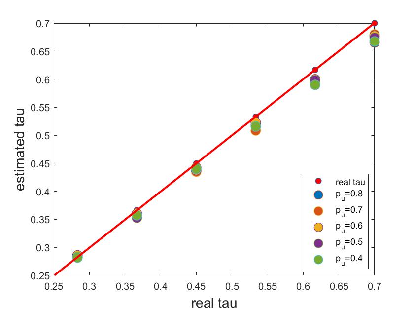
Figure 7: Estimate of the infection parameter $\tau$ for different polynomial random graphs if the number of $SI$ between households is not known. The graph has $N=5000$ vertices, $m=4$, $\gamma=1$; we run five SIR simulations, the dots are averages of the five estimates when $5/6$ of the epidemic events occured. Left: $p_{\rm tr}=0.1$ is fixed; right: $p_{\rm pa}=0.2$ is fixed.

4.1 Parameter estimation with adjustment in the initial period of epidemics

In this section we aim to improve the estimation of the $\tau$ infectious parameter of the virus spread only on some initial phase of the whole process, by applying simulation based adjustment factors in $\hat{E}^{SI,o}_{t}$ the estimated numbers of SI edges outside households. Explicitly, we would like to find some $AdjFact(p_{u},p_{tr},p_{pa})$ adjustment factors, so that with the help of $\hat{E}^{SI,o}_{t}\times(1+AdjFact(p_{u},p_{tr},p_{pa}))$ we get better estimation. The idea was motivated by the following considerations:

• For real life applications, it is more realistic that one would like to estimate the infectious rate right from the beginning of the pandemic, not at the subsidence of the process. With the help of the $\hat{E}^{SI,o}_{t}$ estimation we introduced previously, $\hat{\tau}$ is able to match the real infectious rate on a reasonably long period, however its use is suitable for shorter period of time only to some extent, which is highly depends on the properties of the underlying random graph.

• Based on previous results on $\tau$ convergence (Figure 6) , it can be concluded that generally in the initial period of the virus spread the number of SI edges are under-estimated, while later over-estimated, while the magnitude of error is clearly depends on the structure of the random graph. If we aim to improve the estimation with the help of a single adjustment factor (which can be the function of $p_{u},p_{tr},p_{pa}$ parameters driving the graph structure), it is only possible on some fixed initial period of the virus spread, as this correcting factor would be highly time-dependent.

Driven by the motivations above, firstly we tried to identify a $\tau$ and $p_{u},p_{tr},p_{pa}$ parameter dependent grid of adjustment factors. As first of all, we wanted to grasp independently the pure effect of clustering coefficient and scale free property of the random graph, we created one grid for multiple $p_{tr}$ and $p_{u}$ pairs by keeping $p_{pa}=0$, while in the other grid we bumped $p_{pa}$ and $p_{u}$ with $p_{tr}=0$. In both of the cases we made the following steps: For this simulations, random graphs of $N=5000$ nodes were created from some initial graph of $N_{0}=50$ nodes, with $m=4$ new edges connecting to the existing graph at each step according to the polinomial graph model. (Household layer was added as defined previously with fixed $N_{hh}=5$ number of nodes and weight of 1, while edges outside of the household had weight of $w=0.4$.) The SIR epidemics process was simulated with different $\tau\in[0.3,0.6]$ setups.

1. For each $\tau$ and random graph parameter set, we tried to find the length of the initial period, on which it is possible and considered to be meaningful to improve the the estimation. On each trajectory we calculated the difference between estimated and real SI edges on the whole period, and also the fraction of non-estimated SI edges. Please refer to Figure 8. The length of this initial period was determined as the place of the biggest difference between real and estimated SI edges $len_{max}=\max_{t}\Big{(}\hat{E}^{SI,o}_{t}-E^{SI,o}_{t}\Big{)}$, as based on the simulations the fraction of non-estimated edges locally converges to some value. On each trajectory, we calculated the fraction of this time period regarding to the total epidemic events (infection or recovery), typically 0.1 times the time until the epidemic process stops.

   

   

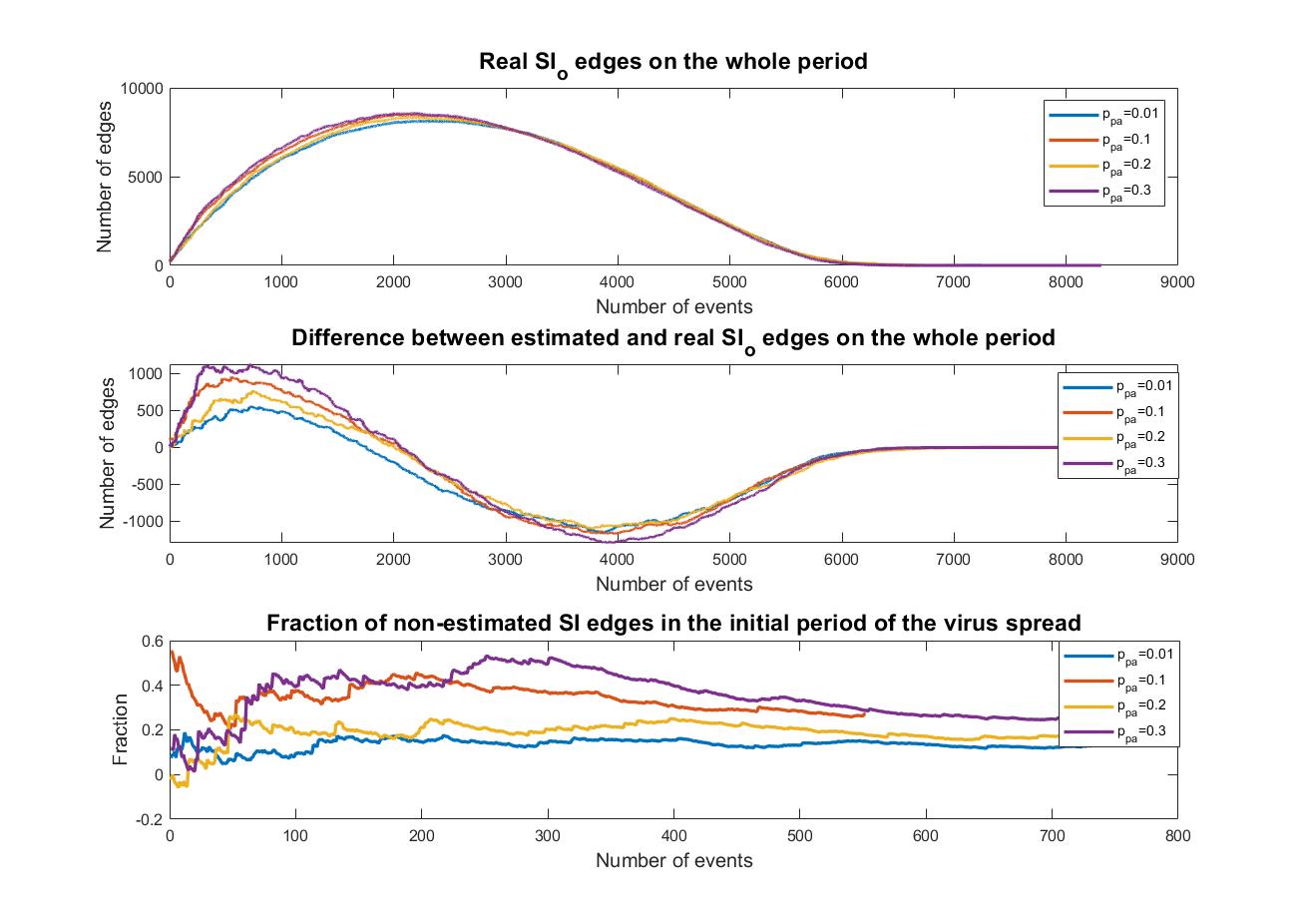
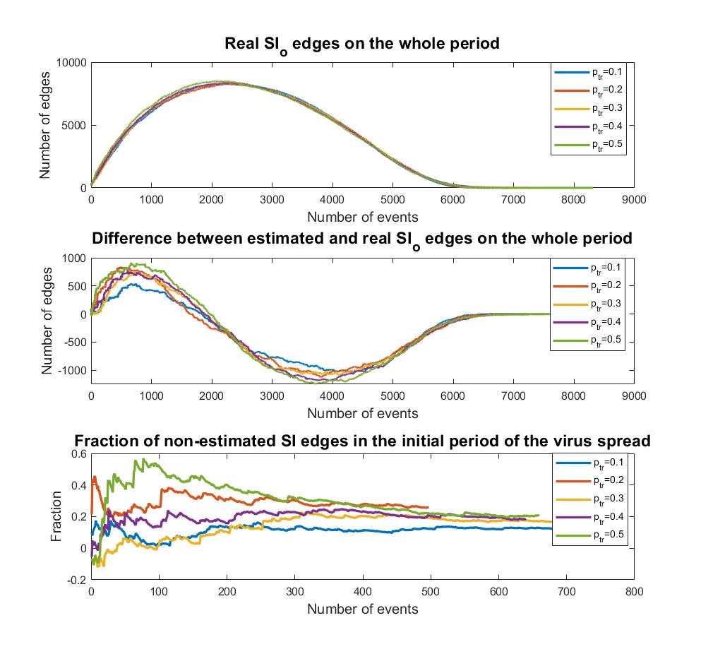
   Figure 8: Error of $\hat{E}^{SI,o}_{t}$ estimation

2. On each testing trajectories calculate the error of our initial estimation, which is the fraction of SI edges the estimation does not take into account $adj(t)=\frac{\hat{E}^{SI,o}_{t}-E^{SI,o}_{t}}{\hat{E}^{SI,o}_{t}}$. Based on the definition of the estimation, it was logical to use the time-integral of $adj(t)$ denoted by $AdjFact(p_{u},p_{tr},p_{pa})=\int_{0}^{len_{max}}adj(s,p_{u},p_{tr},p_{pa})ds$.

3. For each different parameter set we generated 100 random graphs, simulated the virus spread process with some given $\tau$ and calculated the mean of the $AdjFact(p_{u},p_{tr},p_{pa})$ adjustment factors given on each trajectory. As a consequence created a grid, please refer to Figure 9 for the results: It can be concluded that the calculated correcting factors do not depend on $\tau$, therefore the calculated values are meaningful for the improvement of $\tau$ estimation. Adjustment factors are monotonic both in function of $p_{pa}$ and $p_{tr}$ parameters. As expected, the preferential attachment component has very significant effect on the adjustment factors: with $p_{u}=0.7,p_{pa}=0.3,p_{tr}=0$ polinomial graph setup, the original estimation does not take into consideration the quarter of the real $SI_{o}$ edges, as the estimation is based on mean-field theory.

4. For the purpose of backtesting, we calculated the original estimation of $\tau$ infection parameter (similar to Figure 7) based on data of the initial phase of the virus spread and contrasted it to the adjusted estimation. Please refer to Figure 10 for the test results.

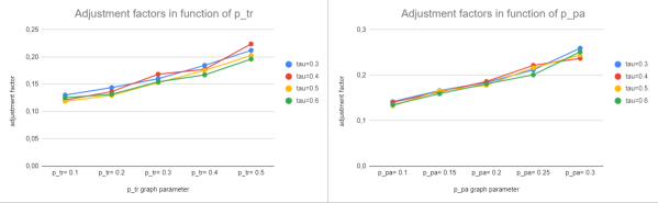
Figure 9: Calculated adjustment factors (mean of 100 independent trajectories) in function of $\tau$ and $p_{tr}$ or $p_{pa}$ parameters

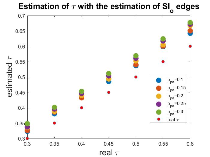
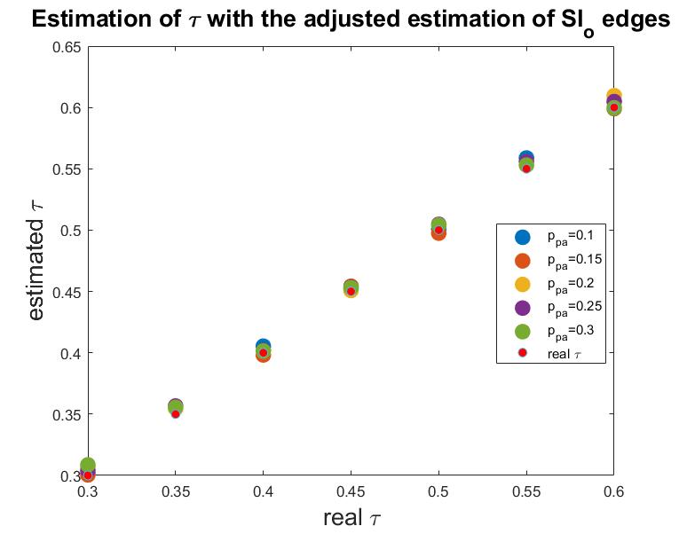
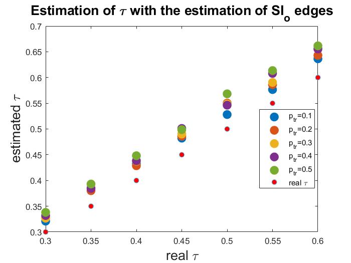
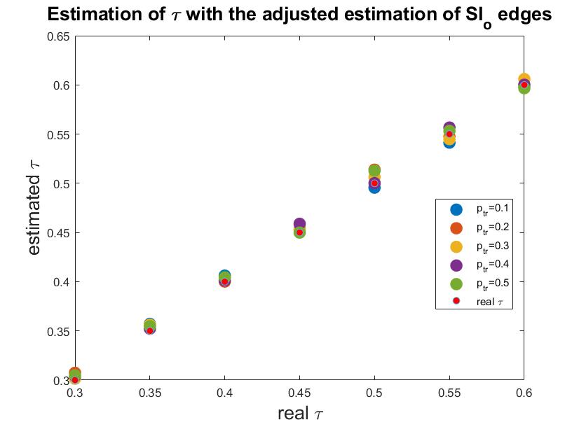
Figure 10: Estimate of the infection parameter $\tau$ for different polynomial random graphs if the number of $SI$ between households is not known with (right) and without adjustment (left). The graph has $N=5000$ vertices, $m=4$, $\gamma=1$; we run 50 SIR simulations, the dots are averages of the 50 estimates when $1/10$ of the epidemic events occured ($p_{\rm tr}=0$ is fixed for the upper figures, while $p_{\rm pa}=0$ is fixed for the lower row).

4.2 Discrete-time SIR process

We also looked briefly at the discrete-time SIR model. If we choose the time unit such that $\gamma=1$, i.e. one time unit is the average time of recovery of an infected individual, then we chose the discretisation step to be $0.05$ time units. For example, if the time unit corresponds to ten days, then the time step of the discrete-time SIR model is half a day. This is small enough to ensure that the results of the continuous-time and the discrete-time epidemic should be very close to each other. Otherwise, we studied the process with the same parameter choices as before, and were interested in the estimation of the between-household SI edges, and in turn the estimation of $\tau$.

We show the results for $\tau=0.3$, and $p_{\rm pa}=0.3,p_{\rm tr}=0.1$. All other characteristics of the setup are the same as in Figure 7. The right panel of Figure 11 shows how the number of SI edges per infected vertex develops over time between households, as well as the estimated value of this quantity. From the figure we can see that the number of between-household SI edges cannot be estimated uniformly well as $C\cdot I_{t}S_{t}$ for some constant $C$, because the number of susceptible vertices decreases monotonically, while the number of SI edges per infected vertex first increases, and later on decreases.

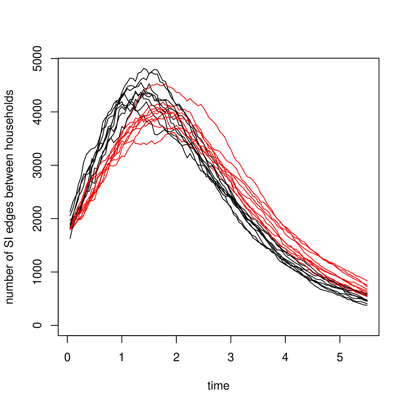
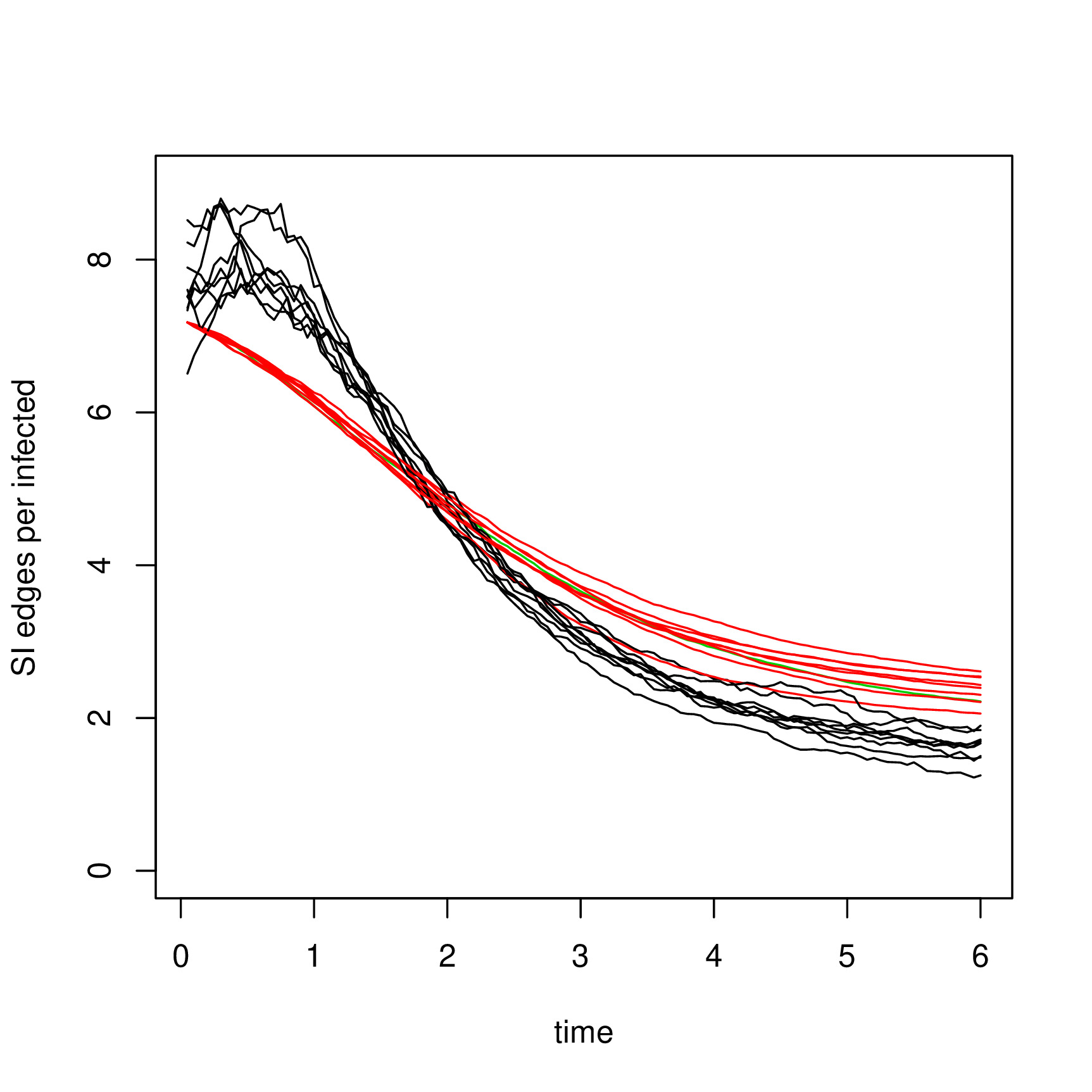
Figure 11: Left: Number of SI edges between households (black) and their estimated number (red). Right: Number of between-household SI edges per infected vertex (black) and their estimated number (red). $N=5000$, $m=4$, $p_{\rm pa}=0.3$, $p_{\rm tr}=0.1$, $\tau=0.3$, $\gamma=1$, three graphs and three SIR simulations on each graph.

From the left panel of Figure 11 one can see that the peak of the estimated number of between-household SI edges is lower than the true value, and also, there seems to be a shift between the two curves. The idea arises to estimate the number of SI edges between households at time $t$ by the formula

$$\hat{E}^{SI,o}_{t}=I_{t+t_{0}}\cdot\bigg{(}d-\frac{wd}{wd+N_{\rm hh}-1}\bigg{)}\cdot\frac{S_{t+t_{0}}}{N},$$ (2)

where $t_{0}$ is a suitably chosen shift. With this method, we need to wait until time $t+t_{0}$ to estimate the contagion parameter $\tau$ at time $t$, but if $t_{0}$ is small, this is not a severe limitation. Figure 12 shows the estimate of $\tau$ with various choices of $t_{0}$. None of the curves seen in the figure perform well overall, but we may say that the shift seems to improve the quality of the estimate. However, the phenomenon would need more careful exploration, and the choice of the shift size is another question.

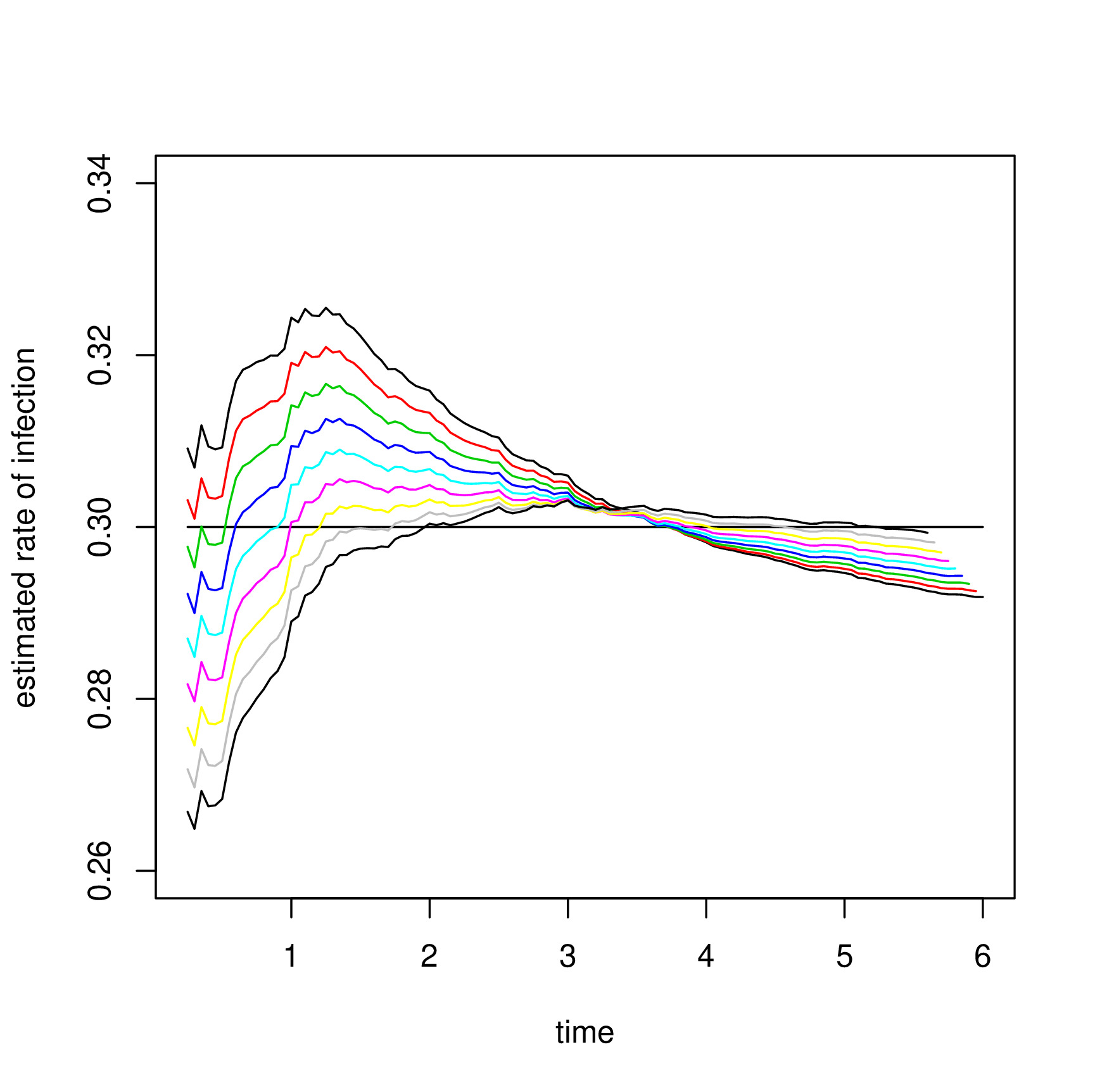
Figure 12: Estimated rate of infection, using the ”shifted” estimate (2) for the number of between-household SI edges. Top curve: no shift, and the shift time grows on the left hand side from top to bottom. Each curve is the average of nine simulations. $N=5000$, $m=4$, $p_{\rm pa}=0.3$, $p_{\rm tr}=0.1$, $\tau=0.3$, $\gamma=1$.

5 Deep learning of contagion dynamics

5.1 The GNN framework

To compare the more traditional maximum likelihood estimation to the neural network approach, we decided to rely on a package developed by Murphy et al., presented in their paper [15]. Although their setup is somewhat different from our starting conditions detailed in the previous sections, we hope that eventually we will be able to modify their architecture to cover our setup as well.

In their paper the authors show how graph neural networks (GNNs), usually used for structure learning, can also be used to model contagion dynamics on complex networks. They design a training procedure and an appropriate GNN architecture capable of representing a wide range of dynamics, which they validate on simulated and real data of increasingly complex contagion dynamics and a variety of network structures.

Now, we review only those results of the cited paper which are most relevant to our research. Assume that an unknown dynamical process takes place on a known network structure, i.e. the graph on which the epidemic spreads is fully known. This includes the vertices and edges of the graph, as well as possible vertex and edge attributes (e.g. weights). The dynamics is assumed to be time invariant, and it acts locally, i.e. the state of a node at the next time step only depends on its current state, and the current states of its neighbors (and on the node and edge attributes of the neighborhood). The objective is to construct a GNN such that after training it on an observed dataset, it mimics the spread of the contagion on any possible graph. The data in this case consists of consecutive snapshots of the epidemic: i.e. we observe how the states of the nodes transition from timestep to timestep.

Therefore, contrary to our approach, [15] works with

• a fully known network,

• discrete time steps,

• general contagion dynamics, which it tries to mimic, instead of just estimate the infection rate.

As mentioned before, the authors investigate a number of contagion dynamics, one of which is the ”simple contagion dynamics” which coincides with our model, where a susceptible node gets the infection from its infected neighbors independently. They show that their GNN architecture can estimate the transition probability $S\to I$ more smoothly than the maximum likelihood method. This is because the MLE is computed for each individual pair $(x,\ell)$ from disjoint subsets of the training dataset (here $x$ is the state of the node and $\ell$ is the number of its infected neighbors). On the other hand, the GNN can interpolate within the dataset, it benefits from any sample to improve all of its predictions, which are then smoother and more consistent.

An important observation regards the network $G$ on which the GNN is trained. Perhaps not surprisingly, a graph with heterogenous degree distribution (e.g. Barabási-Albert graph) offers a wider range of degrees than one whose degree sequence is more homogeneous (e.g. Erdős-Rényi graph), thus a GNN trained on the former generalizes better across a wider range of network structures.

One of our contribution was to define several new network stuctures, and investigate the performance on different training-testing graph pairs – see the next section. The performance was measured using various global loss functions, as in the cited paper.

Let us describe briefly the GNN architecture set up by Murphy and his coauthors. For the simple contagion dynamics, which is most relevant for our present research question, it consists of the following:

• Input layers (Linear(1,32), ReLU, Linear(32, 32), ReLU): these transform the node states and possible node attributes into vectors.

• Attention layers (in this case 2 of them in parallel): these aggregate the node variables with the features of its neighbors, and the possible edge attributes.

• Output layers (Linear(32, 32), ReLU, Linear(32, 2) Softmax): compute the outcomes of the nodes.

This architecture has altogether $6698$ trainable parameters. There are several hyperparameters to be chosen for training the GNN, these include time series length, network size, resampling time, and importance sampling bias. The performance of the neural network depends on all these hyperparameters, so one has to be careful in their choice.

The authors of [15] have also compared their architecture to other ones, and their conclusion is worth citing: ”… not all GNN architectures are capable of learning a dynamical process on networks, which also supports the idea … that most GNN architectures in fact do not have a high expressive power. Then, we can ask if having an extensive aggregator will always be sufficient in the context of dynamical process learning. From our work, it seems to be the case, but the few examples we provide in this paper are far from conclusive in that regard.”

5.2 Deep learning of dynamics for clustered graphs

In this section we present our results regarding the performance of the neural network based approach presented in [15], as a function of average clustering of the network in the epidemic model. As stated before, in the stochastic epidemic model the infection dynamics is a probability distribution of transitioning from a susceptible to infected state, as a function of the number of neighbours (thus it is a function of local structure).
The neural network is trained with generated data from an epidemic model with a given network topology. The proposed goal in [15] is to produce accurate predictions on transition probabilities in any network topology after training the GNN on just one particular topology. The authors found scale-free Barabási-Albert (BA) graphs to provide the best training dataset.
We extended the model to include highly clustered networks (i.e. with asymptotically non-vanishing average clustering coefficient) in both GNN training and testing. The clustered networks possess both scale-free structure and high average clustering according to model presented in Holme et al. 2001 [10]. Although this model is slightly different than the one we used, we chose to use it out of convenience, as Python module NetworkX already contained an algorithm generating graphs based on the model. Here, the graph-generating algorithm differs from the Barabási-Albert model in that an additional triangle-forming step is included after the addition of each new node’s preferential attachment step. The model produces a wide range of average clustering (0-0.7 according to [10]) as a function of a tunable parameter – the triangle forming probability – whilst preserving the scale-free property of the Barabási–Albert model. To fit it to our model used in the MLE-based approach we added a further layer of households to the network consisting of disjoint cliques of a given size ($N_{\rm hh}=5$ as in the previous sections).
We compared the performance of the neural network in cases of training datasets from network models with different average clustering. The performance was evaluated by calculating the $l_{2}$-error of the GNN prediction on contagion dynamics compared to the ground truth provided by the simulated datasets.

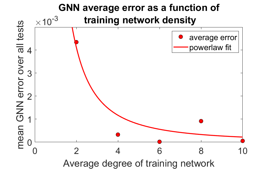
Figure 13: Using BA networks for GNN training, a clear relationship between training network density and GNN performance can be observed.

When using data generated from networks from any model class for GNN training we found a clear relationship between network density and GNN performance as seen in Figure 13. Dense networks offered better training datasets in a given parameter range. Controlling for this parameter, the previously observed relationship between clustering and performance proved to be spurious as seen in Figure 14.

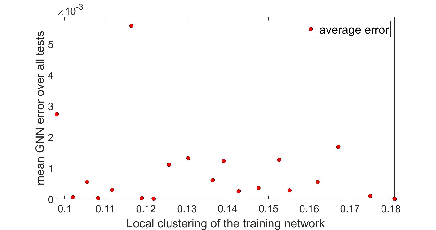
Figure 14: GNN performance as a function of average clustering of the graph generating the training dataset. The average degree of the graphs was fixed ($\overline{d}=13.74$, $\sigma=0.55$).

Evaluating the training using the evaluation function provided by PyTorch, and the cross-entropy value described in [15] (i.e.

$$\mathcal{L}(\mathbf{\Theta})=\sum\limits_{t\in\mathcal{T}^{\prime}}\sum\limits_{v_{i}\in\mathcal{V}^{\prime}(t)}\frac{w_{i}(t)}{Z^{\prime}}L\left(y_{i}(t),\hat{y}_{i}(t)\right),$$

where $\mathbf{\Theta}$ are the GNN parameters, $\mathcal{T}^{\prime}$ and $\mathcal{V}^{\prime}(t)$ are the training time set and node set, $w_{i}(t)$ are importance weights, $Z^{\prime}$ is a normalization factor, $y_{i}(t)$ and $\hat{y}_{i}(t)$ are the real transition probabilities and the GNN output respectively, while $L(y_{i},\hat{y}_{i})=-\sum\limits_{m}y_{i,m}\log\hat{y}_{i,m}$ is the local cross-entropy loss function with $y_{i,m}$ the $m$th element of the output vector) we can observe non-monotonic and nearly constant losses at any stage of the GNN training, while the $l_{2}$ error decreased monotonically as seen in Figure 15. This was the motivation for using the $l_{2}$ metric as a reliable means of evaluation.
We estimated the dependence of network performance on the number of datapoints in the neural network training datasets as a powerlaw with exponent $\beta=-3.6853$ and constant $c=2.4068\cdot 10^{4}$ as seen in Figure 16.

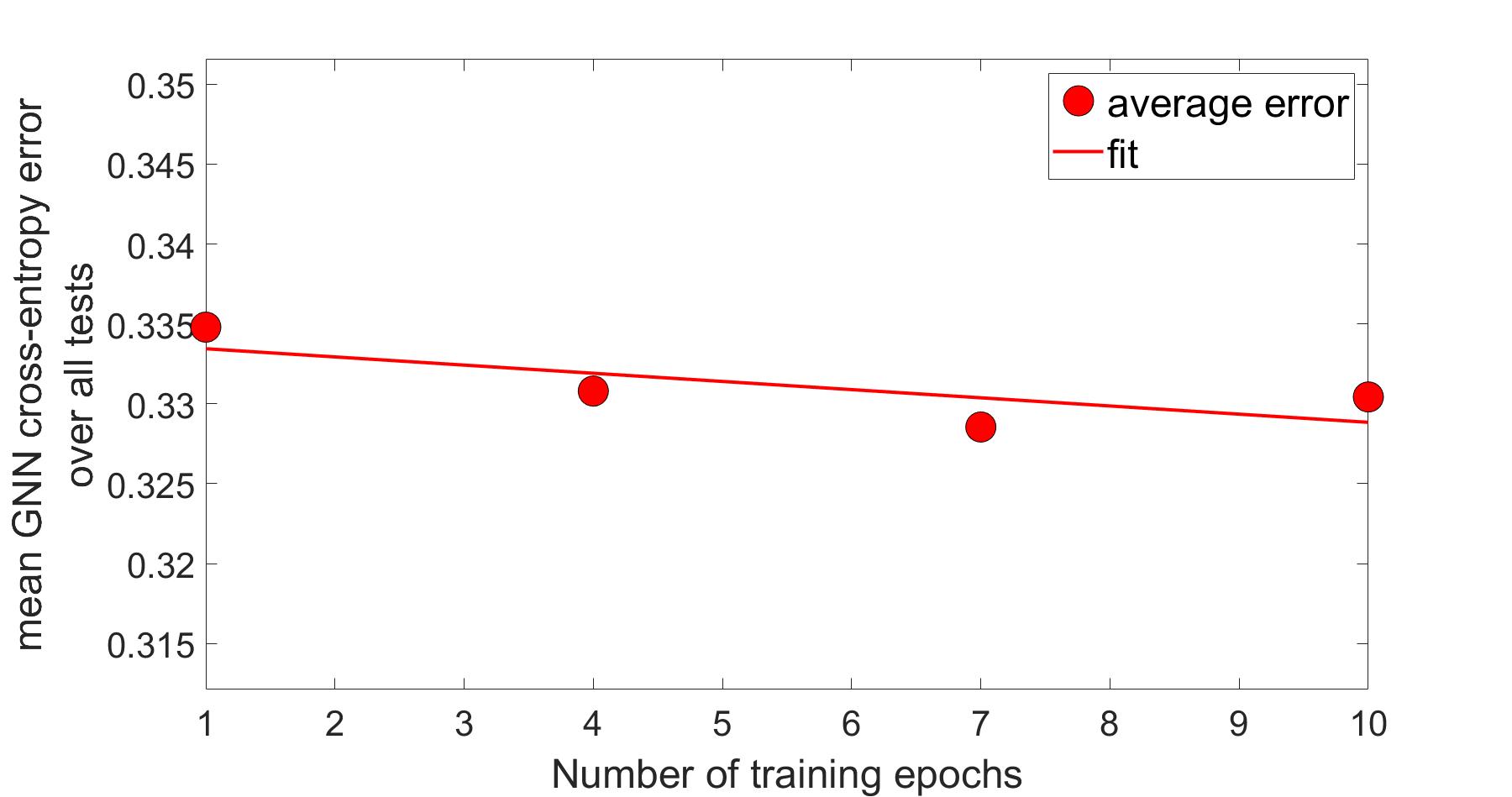
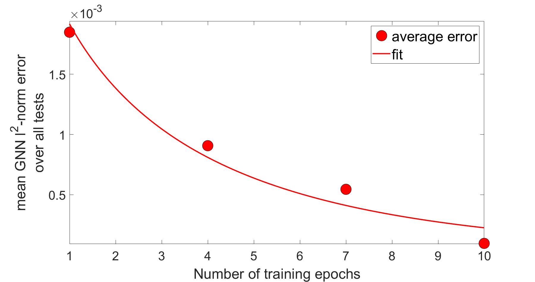
Figure 15: Evaluating GNN performance as a function of the number of training epochs, using the cross-entropy value described in [15] (left), and using $l_{2}$ norm (right). The fitted curve is $y=f(x)=c\cdot e^{\alpha x^{\beta}}$, with $c=5$, $\alpha=-0.5008$ and $\beta=-1.5$ minimizing the mean-squared error of the functional form $f$.

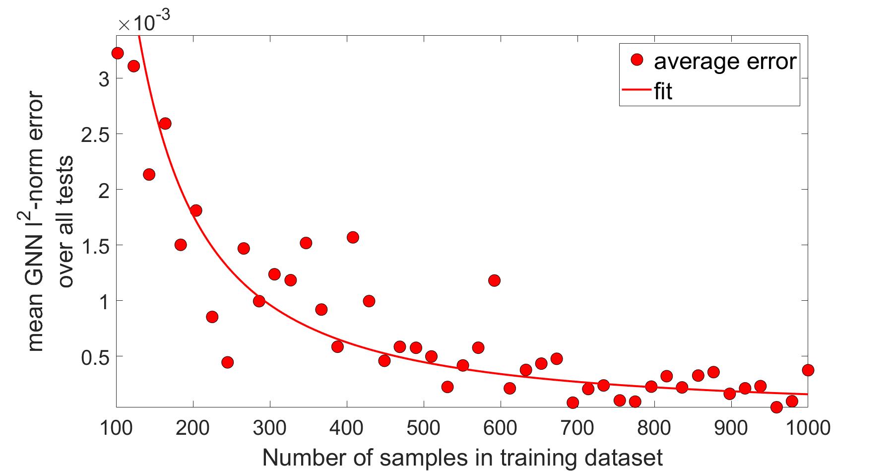
Figure 16: Evaluating GNN performance as a function of the number of datapoints in the training dataset. Featured is the curve $y=f(x)=c\cdot x^{\beta}$, with $c=2.4068\cdot 10^{4}$ and $\beta=-3.6853$ as a function, minimizing mean-squared error of the $f$ functional form.

Conclusions

In this paper we considered a two-layer random graph, consisting of a fixed, deterministic household structure and a preferential attachment model based on [18], added independently. The parameters of the second layer had a significant effect on the degree distribution and the average local clustering coefficient. Given these random graphs with different structural properties, we proposed two methods to estimate the infection parameter in an SIR model. The first, simpler method does not use detailed information about the graph (only quantities like the average degree of a vertex outside its household or the actual number of infected individuals), while the second method is based on a graph neural network, and uses much more detailed information about the graph (e.g. information about the neighbors). Hence, in general, it is not easy to compare the two methods, as they are elaborated for significantly different setups. However, in both cases we may ask whether the structure of the graph (degree distribution, clustering coefficients) has a visible effect on the quality of the estimates.

In the first case we can conclude that increasing the weight of the preferential attachment component, which is closely related to the proportion of vertices with very large degree, leads to larger error in our estimates. As for the GNN method, we observed that the edge density had a significant effect, graphs with larger edge density formed more optimal training sets. On the other hand, the local clustering coefficient does not seem to have a significant effect on the errors of the estimates in either case.

Hence we may conclude that understanding the effect of degree distribution and edge density might be more important than other structural properties, such as the clustering coefficient. On the other hand, it is an open question how we can modify the structure of the neural network such that it works with less detailed information about the network – in this case, we could compare the two methods more directly, to see the advantages and disadvantages better.

References

- [1] Á. Backhausz, E. Bognár, Járványterjedés paramétereinek becslése többrétegű véletlengráf-modellekben. Manuscipt (in Hungarian).
- [2] Á. Backhausz, I. Z. Kiss and P. L. Simon, The impact of spatial and social structure on an SIR epidemic on a weighted multilayer network, Period. Math. Hungar. 85 (2022), no. 2, 343–363. MR4514190
- [3] F. Ball, D. Mollison and G. Scalia-Tomba, Epidemics with two levels of mixing, Ann. Appl. Probab. 7 (1997), no. 1, 46–89. MR1428749
- [4] F. Ball, D. Sirl and P. Trapman, Analysis of a stochastic SIR epidemic on a random network incorporating household structure, Math. Biosci. 224 (2010), no. 2, 53–73. MR2655798
- [5] A.-L. Barabási and R. Albert, Emergence of scaling in random networks, Science 286 (1999), no. 5439, 509–512. MR2091634
- [6] B. Bollobás and O. M. Riordan, Mathematical results on scale-free random graphs. In: Handbook of graphs and networks (editors: S. Bornholdt, H. G. Schuster), 1–34, Wiley-VCH, Weinheim. MR2016117
- [7] T. Britton and P. D. O’Neill, Bayesian inference for stochastic epidemics in populations with random social structure, Scand. J. Statist. 29 (2002), no. 3, 375–390. MR1925565
- [8] T. Britton, Epidemic models on social networks—with inference, Stat. Neerl. 74 (2020), no. 3, 222–241. MR4157131
- [9] M. D’Arienzo, A. Coniglio, Assessment of the SARS-CoV-2 basic reproduction number, R0, based on the early phase of COVID-19 outbreak in Italy, Biosafety and Health 2 (2020), no. 2, 57–79.
- [10] P. Holme, B. J. Kim, Growing Scale-Free Networks with Tunable Clustering, Physical Review E 65 (2001), 026107.
- [11] W. R. KhudaBukhsh, B. Choi, E. Kenah, G. A. Rempała, Survival dynamical systems: individual-level survival analysis from population-level epidemic models. Interface Focus, 10 (2020), no. 1, 20190048.
- [12] I. Z. Kiss, J. C. Miller and P. L. Simon, Mathematics of epidemics on networks, Interdisciplinary Applied Mathematics, 46, Springer, Cham, 2017. MR3644065
- [13] A. Krot and L. Ostroumova Prokhorenkova, Local clustering coefficient in generalized preferential attachment models, in Algorithms and models for the web graph, 15–28, Lecture Notes in Comput. Sci., 9479, Springer, Cham. MR3500665
- [14] T. Kypraios, P. Neal and D. Prangle, A tutorial introduction to Bayesian inference for stochastic epidemic models using approximate Bayesian computation, Math. Biosci. 287 (2017), 42–53. MR3634152
- [15] C. Murphy, E. Laurence, A. Allard, Deep learning of contagion dynamics on complex networks. Nat. Commun. 12 (2021), 4720.
- [16] A. Nande, B. Adlam, J. Sheen, M. Z. Levy, A. L. Hill, Dynamics of covid- 19 under social distancing measures are driven by transmission network structure. PLOS Computational Biology 17 (2021), no. 2, e1008,684.
- [17] D. O’Neill, A tutorial introduction to Bayesian inference for stochastic epidemic models using Markov chain Monte Carlo methods, Math. Biosci. 180 (2002), 103–114. MR1950750
- [18] L. Ostroumova, A. Ryabchenko and E. Samosvat, Generalized preferential attachment: tunable power-law degree distribution and clustering coefficient. In: Algorithms and models for the web graph (editors: K. Avrachenkov, P. Prałat, N. Ye), 185–202, Lecture Notes in Comput. Sci., 8305, Springer, Cham. MR3163720
- [19] A. Tomy, M. Razzanelli, F. Di Lauro, D. Rus, C. Della Santina, Estimating the state of epidemics spreading with graph neural networks, Nonlinear Dyn. (2022), 1–15.
- [20] V. C. Tran, Stochastic epidemics in a heterogeneous community. In: Stochastic epidemic models with inference (editors: T. Britton, E. Pardoux), 239–313, Lecture Notes in Math., 2255, Math. Biosci. Subser, Springer, Cham, 2019. MR4299430
- [21] H. Yin, A. R. Benson, J. Leskovec, The local closure coefficient: A new perspective on network clustering. In: Proceedings of the Twelfth ACM International Conference on Web Search and Data Mining, 303–311, Association for Computing Machinery, New York, 2019.