Mid-infrared fine structure lines from the Galactic warm ionized medium

Abstract

The Warm Ionized Medium (WIM) hosts most of the ionized gas in the Galaxy and occupies perhaps a quarter of the volume of the Galactic disk. Decoding the spectrum of the Galactic diffuse ionizing field is of fundamental interest. This can be done via direct measurements of ionization fractions of various elements. Based on current physical models for the WIM we predicted that mid-IR fine structure lines of Ne, Ar and S would be within the grasp of the Mid-Infrared Imager-Medium Resolution Spectrometer (MIRI-MRS), an Integral Field Unit (IFU) spectrograph, aboard the James Webb Space Telescope (JWST). Motivated thus we analyzed a pair of commissioning data sets and detected [NeII] 12.81 $\mu$m, [SIII] 18.71 $\mu$m and possibly [SIV] 10.51 $\mu$m. The inferred emission measure for these detections is about $10\,{\rm cm^{-6}\,pc}$, typical of the WIM. These detections are broadly consistent with expectations of physical models for the WIM. The current detections are limited by uncorrected fringing (and to a lesser extent by baseline variations). In due course, we expect, as with other IFUs, the calibration pipeline to deliver photon-noise-limited spectra. The detections reported here bode well for the study of the WIM. Along most lines-of-sight hour-long MIRI-MRS observations should detect line emission from the WIM. When combined with optical observations by modern IFUs with high spectral resolution on large ground-based telescopes, the ionization fraction and temperature of neon and sulfur can be robustly inferred. Separately, the ionization of helium in the WIM can be probed by NIRspec. Finally, joint JWST and optical IFU studies will open up a new cottage industry of studying the WIM on arcsecond scales.

1 Introduction

A major challenge in understanding the WIM is the energetics and propagation of Lyman continuum. The inferred ionizing power is high, requiring a sixth or so of the Lyman continuum ($\lambda<912\,$Å, hereafter the Extreme Ultraviolet or EUV) output of the Galactic OB stars (see Haffner et al. 2009 for review; Reynolds 1984). Separately, in order to explain the filling factor, the EUV photons, although originating in the Galactic plane, have to diffuse to nooks and crannies in the Galactic disk. The spectrum of the ionizing photons is significantly modified as they propagate away from star-forming regions. The relative abundance of ions in various ionization states allow us to directly probe the spectrum of the diffuse EUV radiation field.

The traditional diagnostics of the WIM have been optical recombination lines of hydrogen and helium and optical nebular lines of O I, N I, O II, N II, S II and O III. An illustrative example of the richness of the optical lines can be found in Reynolds et al. (2004). The Wisconsin H$\alpha$ Mapper (WHAM; Tufte 1997; Reynolds et al. 1998) was and continues to be the primary workhorse for optical studies of the WIM. It undertook a full-sky H$\alpha$ survey as well as several large-area imagery in [SII] and [NII]. The line ratios (e.g., [SII]/H$\alpha$, [NII]/[SII]) for the WIM are very different from those seen towards bright H II regions.

We summarize the key findings that have emerged from the optical studies. A number of lines of evidence argue for a WIM temperature of 8,000 K to 10,000 K, significantly higher than those of H II regions (5,000 K to 7,000 K; depending on metalicity). Three deep observations of [OI] $\lambda$6300 Å constrain the neutral fraction of hydrogen, thanks to the strong charge exchange, to 10% (Hausen et al., 2002). A single deep observation in [NI] $\lambda$5100 Å constrains the neutral fraction of nitrogen, $n_{\rm N^{0}}/n_{\rm N}\lesssim 0.05$ (Reynolds et al., 1977). The consensus view is that the hydrogen in the WIM is partially ionized, $x_{\rm H^{+}}=n({\rm H^{+}})/n({\rm H})\approx 0.9$. The few observations in the [OIII] provide an upper limit to the temperature of the WIM, $\lesssim 10^{4}\,$K (Reynolds, 1985; Madsen & Reynolds, 2005). The WIM was investigated in [OII] with a novel spectrometer (Mierkiewicz et al., 2006) but no long-term program was undertaken.

The “ionization parameter”, $U$, the ratio of the number density of ionizing photons to the number density of hydrogen atoms, is key to distinguishing classical H II regions from the WIM. The Lyman continuum optical depth to the Strömgren surface, $\tau_{0}\propto U^{1/3}$. Classical H II regions with $\tau_{0}\gg 1$ have sharply defined Strömgren surfaces with gas within the sphere fully ionized. The WIM optical line ratios discussed above have been traditionally modeled by low values of $U$ (Mathis, 1986; Domgörgen & Mathis, 1994; Sembach et al., 2000). Observations of an optical helium recombination line (Reynolds & Tufte, 1995) and extensive and deep radio recombination line studies (Heiles et al., 1996) suggest that helium is weakly ionized, $x_{\rm He^{+}}<0.3$ (optical) or $<0.13$ (radio). This suggests that the diffuse EUV field is relatively “soft”.

Through the fine structure lines of Ne II, Ne III, Ar II, Ar III, S III and S IV, and recombination lines of hydrogen and helium the mid-IR offer new diagnostics of the WIM. The recently launched James Webb Space Telescope (JWST) carries two spectrometers: the Near Infrared Spectrograph (NIRSpec; Böker et al. 2022; Jakobsen et al. 2022) covering the wavelength range 1–5 $\mu$m while the Mid-Infrared Instrument-Medium Resolution Spectrograph (MIRI-MRS; Wells et al. 2015; Labiano et al. 2021) covers 5–29 $\mu$m. JWST, with its narrow spectroscopic field-of-view (FoV, $\Omega$ ranging from ten to fifty arcsec²) is not an obvious facility of choice to study diffuse emission from Galactic WIM. However, at turns out, this small FoV is compensated by the large collecting area of JWST, efficient integral field unit (IFU) spectrometers with spectral resolution of few thousand (Wells et al., 2015) and a thousand spaxels and detectors with negligible dark current (Ressler et al., 2015).

The paper is organized as follows. In §2 we introduce the mid-IR fine structure lines and summarize their potential diagnostic value. In §3 we investigate the detectability of mid-IR fine structure lines with MIRI-MRS. Buoyed by the conclusions of our study we analyzed MIRI-MRS commissioning data sets. In §4 we present secure detections of Ne II and S III and possibly S IV detection from the WIM. In §5 we find the detections are consistent with the low-$U$ photoionization models invoked for the WIM. We conclude in §6 by first noting that hour-long MIRI-MRS observations will, for many lines-of-sight, detect of [NeII], [ArII] and [SIII] from the WIM. Thus, there will be a steady growth of measurements of the WIM ionization fractions. We discuss the detectability of ionized helium with NIRSpec. We end by noting the great returns that would be made possible by joint studies undertaken with JWST & ground-based high spectral-resolution IFU spectrographs.

Unless otherwise mentioned, all basic formulae, collisional and recombination coefficients are from Draine (2011) and the atomic data (A-coefficients, wavelengths) from NIST.

2 The Mid-IR Fine Structure Lines

In the optical, line ratios have been used to infer the temperature and study the state of ionization. For instance, WHAM observations of variation in [NII]/[SII] is nicely explained by variation in $x_{\rm S^{+}}$ from 0.3 to 0.8 while variations in [NII]/H$\alpha$ are readily explained by temperature variations, from 6,000 K to 10,000 K (Haffner et al., 1999). Next, the low value of $x_{\rm S^{++}}$ (inferred from [SIII] observations) is suggestive of the softening of the diffuse EUV field even at photon energies as low as 23 eV.

The mid-IR lines, unlike the optical lines, are not sensitive to variations in temperature and furthermore suffer much less from extinction (including reflection). As will become clear from the discussion below they are also well suited to probing the ionization state.

Of the elements with more than one part million (ppm), Ne, Ar and S have mid-IR lines that are accessible to JWST. As can be seen from Table 1 the ionization potentials of Ne, Ar and S are well suited to probing the spectrum of the diffuse EUV radiation field above the H I and He II edges. Below we develop the formulae for intensities of the mid-IR fine structure lines. The fine structure splitting of [NeII], [ArII] and [SIV] results in two levels but [NeIII], [ArIII] and [SIII] have three levels. Note that [NeIII] 30.01 $\mu$m and [SIII] 33.48 $\mu$m lie outside the wavelength range of MIRI-MRS and so are dropped from any further discussion. The relevant atomic physics data can be found in Appendix A.

Table 1: Ionization Potential

$X$	$Y_{X}$ (ppm)	I$\rightarrow$II	II$\rightarrow$III	III$\rightarrow$IV
Ne	93.3	21.6	41.0	63.4
S	14.5	10.4	23.3	34.8
Ar	2.75	15.8	27.6	40.7
N	74.1	14.5	29.6	47.4

Note. — $X$ is element and $Y_{X}$ is the abundance by number, relative to hydrogen, in parts per million (ppm). Subsequent columns are ionization potential in eV. Nitrogen is included as a point of comparison to argon. For reference, the ionization potential of helium is 24.587 eV.

2.1 Neon

The [NeII] $12.813\,\mu$m fine structure line arises from the spin-orbit splitting of the ${}^{2}{\rm P}^{o}$ ground term. For simplicity we assume that the electrons are provided only by the ionization of hydrogen, $n_{e}=n_{\rm H^{+}}$. The rate of electron excitations per unit volume is $C=n_{\rm H^{+}}n_{\rm Ne^{+}}q_{lu}$ where

$$q_{lu}=\frac{8.629\times 10^{-8}}{T_{4}^{1/2}}\frac{\Omega_{ul}}{g_{l}}{\rm e}^{-T_{u}/T}\,{\rm cm^{3}\,s^{-1}}$$

is the electron collisional coefficient, $g_{l}$ is the degeneracy factor of the lower level; $\Omega_{ul}$ is the collisional strength and is given in Table 6; and $T_{u}=E_{u}/k_{B}$ with $E_{u}$ being the energy level difference between the upper and the ground state. The photon intensity is $\int Cdl/(4\pi)$, the integral along the line-of-sight,

$$I_{\rm[NeII]} = 1.95\xi_{\rm Ne^{+}}T_{4}^{-0.424+0.002\,{\rm ln}T_{4}}{\rm e}^{-0.112/T_{4}}{\rm EM}\ R$$ (1)

where $\xi_{\rm Ne^{+}}=x_{\rm Ne^{+}}/x_{\rm H^{+}}$ and ${\rm EM}=\int n_{\rm H^{+}}^{2}dl$ is the emission measure carrying the unit of ${\rm cm^{-6}\,pc}$ and $R$ stands for Rayleigh. For reference, the EM from the WIM varies from $1\,{\rm cm^{-6}\,pc}$ (Galactic poles) to $25\,{\rm cm^{-6}\,pc}$ (the “brightest” WIM region; see Madsen et al. 2006). For the WIM, we assume a fiducial temperature of 8,000 K. At this temperature, $I_{\rm Ne^{+}}=1.86\,{\rm EM}\,R$.

For Ne III, excitation from the ground level to the first and second levels result in emission of 15.555 $\mu$m photons. The intensity of the 15.555 $\mu$m line is given by the sum of the excitations:

$$I_{\rm[NeIII]}=\xi_{\rm Ne^{+2}}\Big{[}3.85T_{4}^{-0.432-0.0556\,{\rm ln}\,T_{4}}\,{\rm e}^{-0.0925/T_{4}}+\\ 1.03T_{4}^{-0.440-0.053\,{\rm ln}\,T_{4}}\,{\rm e}^{-0.1324/T_{4}}\Big{]}\,{\rm EM}\,R$$

with $\xi_{\rm Ne^{+2}}=x_{\rm Ne^{+2}}/x_{\rm H^{+}}$, and, as before, the atomic data can be found in §A. At the fiducial temperature, $I_{\rm[NeIII]}\approx 4.73\xi_{\rm Ne^{+2}}\,{\rm EM}\,R$.

2.2 Argon & Sulfur

In a similar manner the intensities of fine structure lines of argon and sulfur (§A) can be computed:

$$I_{\rm[ArII]} = 0.72\xi_{\rm Ar^{+}}T_{4}^{-0.416-0.014{\rm ln}\,T_{4}}{\rm e}^{-0.206/T_{4}}\,{\rm EM}\,R\ ,$$

$$I_{\rm[ArIII]} =\xi_{\rm Ar^{+2}}\Big{[}0.59T_{4}^{-0.469+0.002{\rm ln}\,T_{4}}{\rm e}^{-0.1601/T_{4}}$$

$$\ \ +0.15T_{4}^{-0.389-0.009{\rm ln}\,T_{4}}{\rm e}^{-0.2259/T_{4}}\Big{]}{\rm EM}\,R\ ,$$

$$I_{\rm[SIII]} = 30.4\xi_{\rm S^{+2}}T_{4}^{-0.671-0.033{\rm ln}\,T_{4}}{\rm e}^{-0.1199/T_{4}}\,{\rm EM}\,R\ ,$$

$$I_{\rm[SIV]} = 16.5\xi_{\rm S^{+3}}T_{4}^{-0.512-0.076{\rm ln}\,T_{4}}{\rm e}^{-0.1369/T_{4}}\,{\rm EM}\,R\ .$$

Table 2: Detectability with MIRI-MRS

species	$\lambda$	ChB	$\mathcal{R}$	$\theta^{\prime\prime}$	$\eta$	$B_{\nu}$	$\sigma\,(R)$	$S/{\rm EM}\,(R)$	$S/\sigma$
[NeII]	12.81	3A	2880	6.1	0.11	30	0.17	$1.85\xi_{\rm Ne^{+}}$	$10.9\xi_{\rm Ne^{+}}{\rm EM}$
[NeIII]	15.55	3B	2560	6.1	0.11	60	0.25	$4.73\xi_{\rm Ne^{+}2}$	$18.8\xi_{\rm Ne^{+2}}{\rm EM}$
[ArII]	6.98	1C	3300	3.7	0.14	3	0.07	$0.91\xi_{\rm Ar^{+}}$	$12.5\xi_{\rm Ar^{+}}{\rm EM}$
[ArIII]	8.99	2B	2850	4.6	0.13	5	0.08	$0.66\xi_{\rm Ar^{+2}}$	$7.8\xi_{\rm Ar^{+2}}{\rm EM}$
[ArIII]	21.83	4B	1700	7.8	0.02	300	1.27	$0.12\xi_{\rm Ar^{+2}}$	$0.09\xi_{\rm Ar^{+2}}{\rm EM}$
[SIII]	18.71	4A	1610	7.8	0.03	160	0.78	$30.33\xi_{\rm S^{+2}}$	$39.0\xi_{\rm S^{+2}}{\rm EM}$
[SIV]	10.51	2C	3000	4.6	0.134	20	0.16	$15.52\xi_{\rm S^{+3}}$	$96.1\xi_{\rm S^{+3}}{\rm EM}$

Note. — The wavelength, $\lambda$, is in microns. “ChB” refers to Channel-band combination. The spectral resolution, $\mathcal{R}=\lambda/\Delta\lambda$ and the side-length of the IFU field-of-view, $\theta$, are from Table 1 of Wells et al. (2015) while $\eta$ is from Table 5 of Wells et al. (2015). $B_{\nu}$ is a rough estimate of the net background emission in MJy ster^-1. $\sigma$ is the Poisson uncertainty due to the background, assuming $t=3600\,s$ of integration time, in a spectral channel carrying the unit of Rayleigh. In computing $S$, the signal strength in Rayleigh, we set $T=8,000\,$K, Note that $\xi_{\rm X}=x_{\rm X}/x_{\rm H^{+}}$ where $x_{\rm X}$ is the ionization fraction of species $X$. EM is the emission measure along the line-of-sight (unit: cm^-6 pc). The last column is the expected signal-to-noise ratio.

2.3 Ionization Fraction

In order to infer the ionization fraction of, for instance [NeII], we need to know the emission measure. The case B H$\alpha$ photon intensity is given by

$$I_{\rm H\alpha}=0.361T_{4}^{-0.942-0.031\,{\rm ln}\,T_{4}}\,{\rm EM}\,R\ .$$

The ratio

$$\frac{\rm[NeII]}{\rm H\alpha}\equiv\frac{I_{\rm Ne^{+}}}{I_{\rm H\alpha}}=5.4\xi_{\rm Ne^{+}}T_{4}^{0.518+0.033{\rm ln}\,T_{4}}{\rm e}^{-0.112/T_{4}}$$

is a direct measure of $\xi_{\rm Ne^{+}}$. Notice, relative to similar ratios involving forbidden optical lines, the ratio (above) is a weak(er) function of temperature. The primary source of H$\alpha$ data is from WHAM which has a beam of one degree diameter while the MIRI-MRS FoV is about ten arcsec² (see Table 2). There is no reason to believe that the WIM is smooth on scales of a degree. We will return to this important point in the concluding section.

Table 3: Summary of log of data sets forHD 163466

name	$\alpha$ (deg)	$\delta$ (deg)	series	$\tau$(s)
HD163466	268.1057	60.396	jw01050-o009_t004	10,930
HD-BKG1	268.0731	60.418	jw01050-o008_t011	1,682
HD-BKG2	268.0731	60.418	jw01050-o010_t011	1,682

Note. — The “name” is our assigned name for the data set. The next two columns are J2000 right ascension and declination, followed by file name identifier of Level-3 MIRI-MRS pipeline data sets. Each data set has four files, one for each channel. For instance, for HD-BKG1, the data cube for the first channel is jw01050-o010_t011_ch1-longshortmedium-_s3d.fits while that for the second channel is jw01050-o010_t011_ch2-longshortmedium-_s3d.fits and so on. The last column is the integration time. The program ID (PID) for these data sets is 1050.

3 Detectability with MIRI/Medium Resolution Spectrometer

The Medium Resolution Spectrometer is an integral field unit (IFU) spectrograph with a spectral resolution, $\mathcal{R}=\lambda/{\rm FWHM}$ of 2000 to 3000 (Wells et al., 2015; Labiano et al., 2021); here FWHM is the full-width at half-maximum of an unresolved line. The instrument is quite complex with four simultaneous channels (1–4) and three selectable bands (A, B, C). The full wavelength range, 4.87–28.82 $\mu$m, is covered by successively going through the three bands. The entrance aperture of the IFU is approximately a square of side $\theta$ which varies from $3.7^{\prime\prime}$ (Channel 1) to $7.8^{\prime\prime}$ (Channel 4). The “photon-photoelectron conversion” efficiency (i.e., the net throughput of the telescope, spectrometer optics and quantum efficiency of the detectors), $\eta$, and $\mathcal{R}$ depend on the channel-band combination. The instrumental parameters are summarized in Table 2. We assume that the detector dark current is negligible.

Our goal is to measure the mid-IR spectrum of the sky and we do so by using MRS as a “light bucket”. The background intensity, $B_{\nu}$, is usually quoted in units of MJy ster^-1 and arises from a combination of thermal emission from the local zodiacal dust cloud and at wavelengths long-ward of $\sim$15 $\mu$m, self-emission from the telescope. Between 5 and 15 $\mu$m the background intensity increases from 0.5 to 50 MJy ster^-1. Then the rate of photo-electrons from the background in one spectral resolution element, frequency width $\Delta\nu\approx\nu/\mathcal{R}$, is $(B_{\nu}/h\mathcal{R})A\Omega\eta$ where $A=25.4\,{\rm m}^{2}$ is the collecting area of JWST and $\Omega=\theta^{2}$. The thermal line width is a few km s^-1. Including Galactic rotation, the expected [NeII] line will be effectively confined to an effective spectral channel (but the FWHM, depending on wavelength, is spread between 2 and 4 pixels; see Figure 14 of Wells et al. 2015). Because the zodiacal and/or telescope emission is smooth both spatially across a few arcseconds and across a few spectral channels, background subtraction to reveal a spectral line should be photon-noise limited once detector calibration issues are fully resolved.

The rate of photo-electrons due to line emission from the WIM is $SA\Omega\eta$ where $S$ is the line photon intensity (${\rm phot\,cm^{-2}\,ster^{-1}\,s^{-1}}$). The SNR of the line is then

$${\rm SNR}=\frac{S}{\sqrt{B_{\nu}/h}}\Big{(}A\Omega\eta\mathcal{R}t\Big{)}^{1/2}$$ (2)

where $t$ is the integration time. In Table 2 we summarize the detectability by MRS. We also list the specific channel-band in which these lines can be observed. As can be gathered from this Table, detections and useful upper limits can be obtained for all species provided that the EM is greater than a few units.

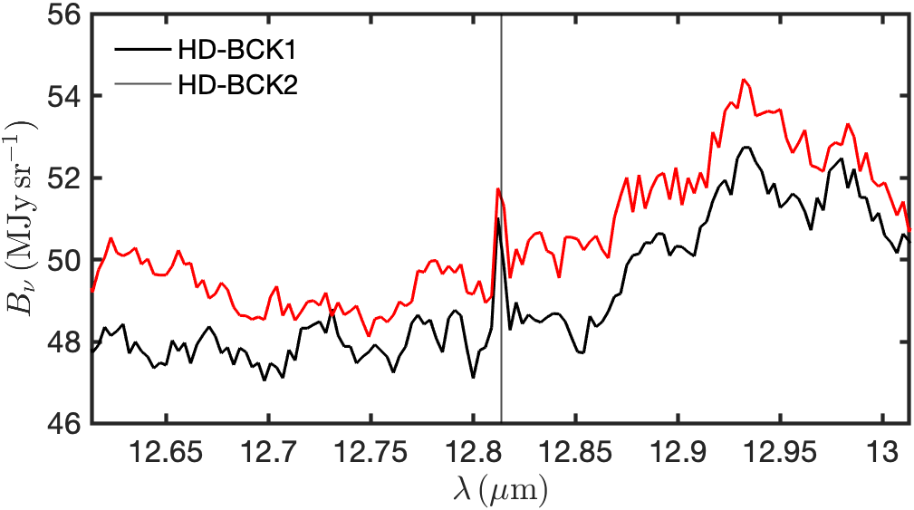
Figure 1: The spectra of the sky, in the vicinity of the [NeII], from data sets HD-BCK1 and HD-BCK2, obtained by taking the median of each of the image slices. The dotted vertical line is the rest wavelength of the [NeII] line.

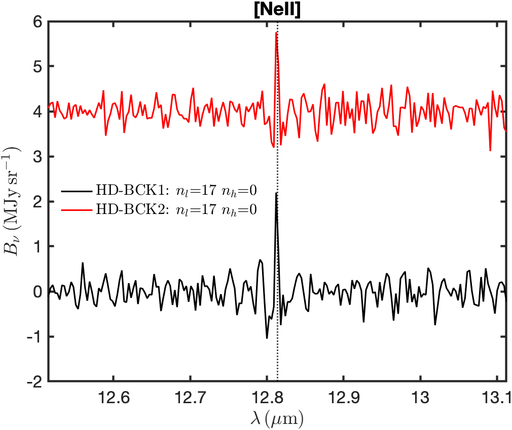
Figure 2: The same as in Figure 1 but after Fourier filtering. The HD-BKG2 spectrum (top) is offset from HD-BKG1 by $4\,{\rm MJy\,sr^{-1}}$. For Fourier filtering the starting point was a a spectrum 200-points long and centered on the line. Following Fourier transform the power spectrum was inspected. The first $n_{l}$ Fourier channels (low frequency) and last $n_{h}$ channels (high frequency) were zeroed out and inverse transform was applied to yield the filtered spectrum displayed here; the values of $n_{l}$ and $n_{h}$ are noted in the figure.

4 Detection by MIRI-MRS

Motivated by the results presented in Table 2 we undertook analysis of MIRI-MRS commissioning data, specifically of a calibration star (HD 163466) and its associated background or “blank” field observations (hereafter, HD-BKG1 and HD-BKG2). The Galactic coordinates of HD 163466 is $l=89^{\circ}.24$ and $b=30^{\circ}.56$. The blank field is some $1.32^{\prime}$ North of HD 163466. The observing log is summarized in Table 3. Summary information on HD 163466 can be found in Appendix B. As a cross-check of our analyses (e.g., in confirming inferred velocities and velocity widths) we also analyzed observations of the bright planetary nebula NGC 6543. The observing log and the analysis of NGC 6543 is summarized in Appendix C.

For all targets, we downloaded the Level-3 MIRI-MRS pipeline data cubes. As a part of the pipeline reduction the MIRI-MRS pipeline wavelength scale has been adjusted to the solar system barycenter. The data sets are cubes with images of size ($n_{x},n_{y}$) and $n_{ch}$ equally spaced (in wavelength) spectral channels. These numbers vary with channel (and dithering pattern) but are typically about (30, 30) and 2000, respectively.

4.1 Background datasets (HD-BKG1, HD-BKG2)

In this sub-section we present our analysis of HD-BKG1 and HD-BGK2 data sets (see Table 3). For each data set the sky spectrum is obtained by taking median of each image slice. In Figure 1 we display the resulting spectrum centered around [NeII] line. There seems to be a clear detection of an unresolved line close to the rest wavelength of the [NeII] line. However, it is clear from the Figure, the sky spectrum is dominated by systematics. After inspection of this spectrum and other spectra it became clear that the systematics are due to three reasons: (i) periodicity in the baseline, (ii) strong pixel-to-pixel variations and (iii) occasionally artifacts, specifically super bright resolved lines.

The signal we are searching is an unresolved line. The Fourier amplitude spectrum of an unresolved line is flat with Fourier frequency. This suggests a Fourier filtering scheme which removes the periodic lumps in the baseline via low-frequency filtering while pixel-to-pixel variation is removed by high frequency filtering.

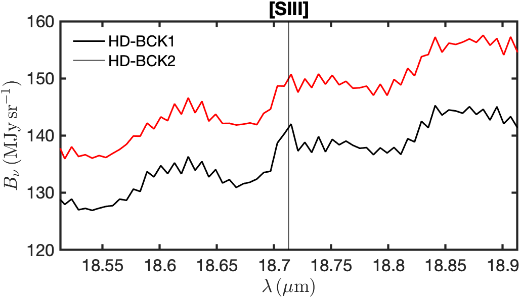
Figure 3: The spectra of the sky, in the vicinity of the [SIII], from data sets HD-BCK1 and HD-BCK2, obtained by taking the median of each of the image slices. The dotted vertical line is the rest wavelength of the [SIII] line. No vertical offsets were applied to the spectra. The variation is presumably due to incomplete calibration.

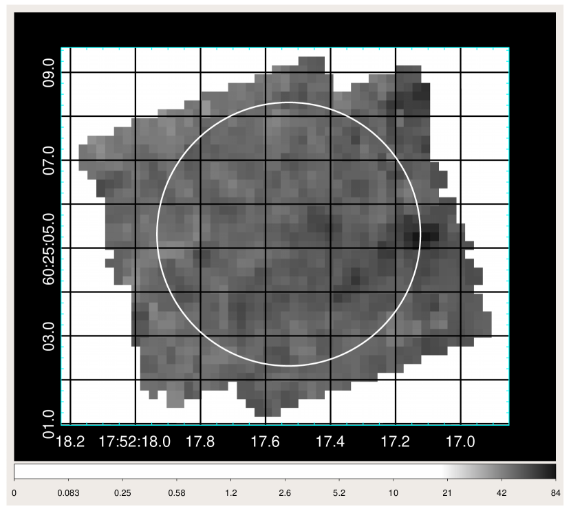
Figure 4: The sky image of the background region in the [NeII] 12.8 $\mu$m line. The sky coordinates are shown in green. A circle with a radius of $3^{\prime\prime}$ is shown for scale.

As can be seen from Figures 1 and 2 the [NeII] line is convincingly detected in the input spectrum and the filtered spectrum. Both detections yield a similar value for the strength of the line. We preferred to use the filtered spectrum to measure the strength of the signal. To this end, based on the window function used for Fourier filtering, we synthesized a “dirty beam”, $f_{D}(\lambda)$. We normalized this profile as follows: $f(\lambda)=f_{D}(\lambda)/\int f_{D}^{2}(\lambda)d\lambda$. We convolved the filtered spectrum with $f(\lambda)$. The line strength was set by the maximum amplitude. We find the resulting line strength to be $2.54\pm 0.31$ (HD-BCK1) and $2.08\pm 0.30\,{\rm MJy\,sr^{-1}}$ (HD-BCK2); here, the rms was determined from the fluctuations in the convolved spectrum (whilst avoiding the line itself). We adopt $2.31\pm 0.30\,{\rm MJy\,sr^{-1}}$. Note that in Table 2 the definition of the spectral resolution incorporates the line width of an unresolved line, $\mathcal{R}=\lambda/{\rm FWHM}$. Thus, the brightness in Rayleigh is $B_{\nu}/(h\mathcal{R})$ and this amounts to $15.2\pm 2.0\,R$. The image of the sky in the [NeII] line is shown in the left panel of Figure 4.

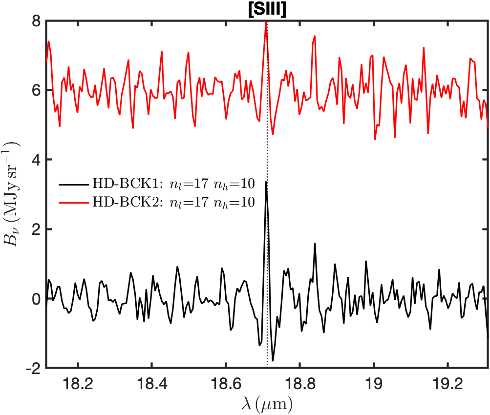
Figure 5: The same as in Figure 3 but after Fourier filtering. The HD-BCK2 spectrum (top) is offset from HD-BCK1 by $6\,{\rm MJy\,sr^{-1}}$.

As can be seen from Figure 3, relative to that of [NeII], the pixel-to-variation for [SIII] is severe. Nonetheless, by eye one can see a line at the rest velocity of [SIII]. As can be seen from Figure 5 the Fourier filtering nicely attenuates the pixel-to-pixel variations and flattens the baseline. The resulting line strengths are $3.70\pm 0.54\,{\rm MJy\,sr^{-1}}$ and $1.96\pm 0.62\,{\rm MJy\,sr^{-1}}$ which leads to a formal value of $2.83\pm 0.58\,{\rm MJy\,sr^{-1}}$. The corresponding surface brightness in the [SIII] line is $33.3\pm 6.8\,R$.

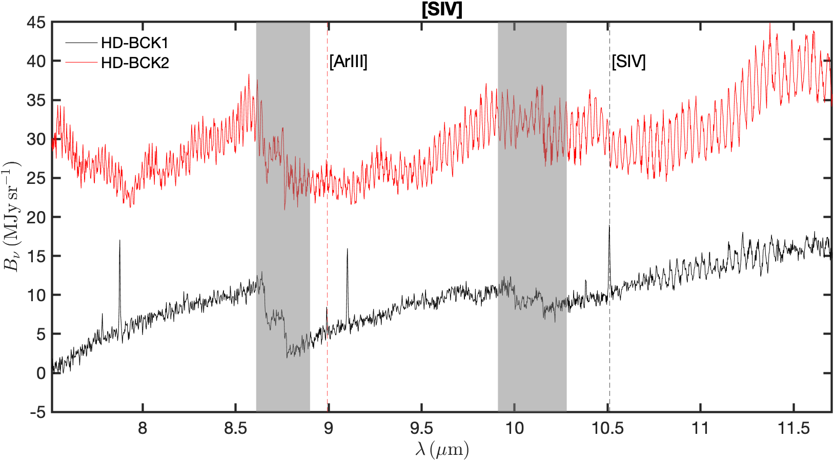
Figure 6: The spectra of the sky of Channel 2 (sub-bands A, B, C) of the data sets, HD-BKG1 and HD-BKG2. The gray columns mark the overlap between adjacent sub-bands (as in A-B and B-C). Notice a pair of bright resolved lines in each of the sub-bands which is present in HD-BKG1 (bottom) but not HD-BKG2 (top). In each band, the separation is about $0.012\lambda$ with $\lambda$ being measured in microns. The wavelength of [SIV] and [ArIII] are marked by vertical lines.

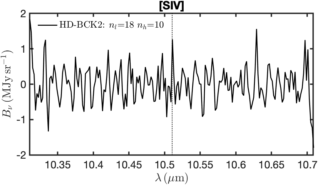
Figure 7: The Fourier-filtered spectrum of the sky, in the vicinity of the [SIV] from HD-BCK2 data set. The dotted vertical line is the rest wavelength of the [SIV] line.

Next we consider [SIV]. As can be seen from Figure 6 the sky spectrum of the first epoch exhibits a pair of bright lines in each of the three bands. These lines are not present in the second epoch. Furthermore, two of these lines coincide with [ArIII] and [SIV]! We suspect that these three pairs of lines are an artifact of the calibration process. We drop data set HDBCK-1 from further analysis. The spectrum emerging from the analysis of HDBCK-2 is shown in Figure 7. The inferred [SIV] line intensity is $1.67\pm 0.66\,{\rm MJy\,sr^{-1}}$ which corresponds to $10.6\pm 3.6\,R$. No other lines were detected with any significance.

The summary of the detections and non-detections can be found in Table 4.

Table 4: Line Strengths

line	$B_{\nu}$ (BKG-1)	$B_{\nu}$ (BKG-2)	$I\,(R)$
[NeII]	$2.54\pm 0.31$	$2.08\pm 0.30$	$15.2\pm 2.0$
[NeIII]	$0.63\pm 0.76$	$1.37\pm 0.55$	$7.4\pm 4.9$
[ArII]	$0.97\pm 0.77$	$1.00\pm 0.79$	$5.7\pm 4.5$
[ArIIIa]	-	$0.60\pm 0.58$	$4.0\pm 3.9$
[ArIIIb]	$1.57\pm 1.09$	$0.44\pm 1.15$	$11.2\pm 12.5$
[SIII]	$3.70\pm 0.54$	$1.96\pm 0.62$	$33.3\pm 6.8$
[SIV]	-	$1.67\pm 0.57$	$10.6\pm 3.6$

Note. — BKG-1 and BKG-2 refer to the two background data sets. The unit of $B_{\nu}$ is ${\rm MJy\,sr^{-1}}$. The last column is the line intensity (unit: Rayleigh, $R$) obtained by taking the arithmetic mean of the two intensities (when available).

4.2 HD 163466 data set

The data set for HD 163466 is attractive because of the long exposure time (see Table 3). However, this is compensated by scattered light from HD 163466 which is a bright star, $V=6.85\,$mag. To this end, we masked out a circular region centered on the star (see Figure 8) and then determined the median of the remaining pixels. The larger the radius of the masked region the smaller is the contribution of the light scattered from the star to the sky spectrum but at the cost of fewer data points. For this reason the analysis was undertaken for two different radii (see Figure 8). The results are summarized in Table 5. [NeII] is robustly detected at $\approx 1.9\,{\rm MJy\,sr^{-1}}$ and [SIII] is plausibly detected, $S\approx 4\,{\rm MJy\,sr^{-1}}$. The corresponding photon intensities are $12\pm 2\,R$ and $47\pm 15\,R$. Within errors both are consistent with the determinations from the background fields.

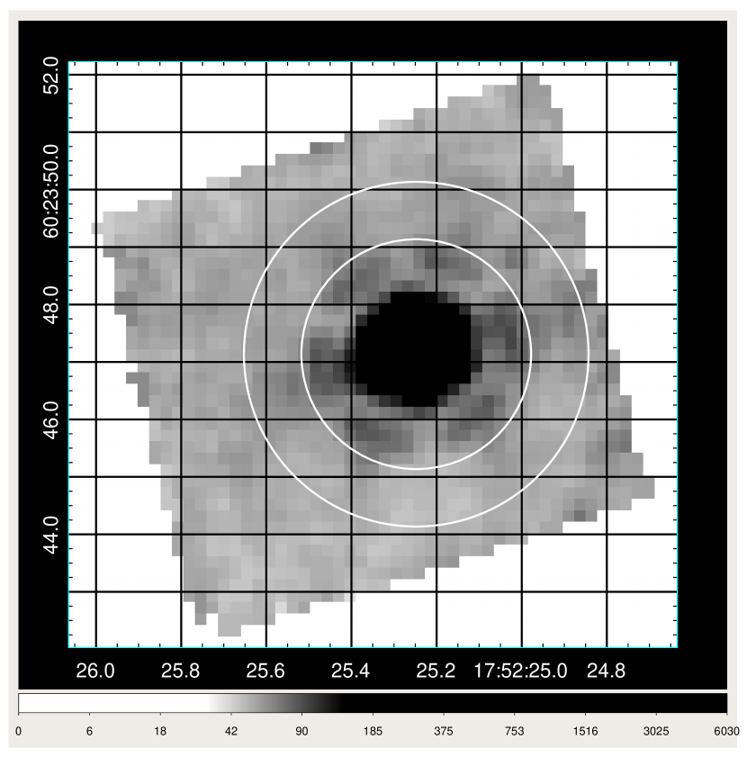
Figure 8: The sky image centered on HD 163466. The circles define 10 and 15-pixel radius masks used to reject light from the aperture around the star HD 163466 (see text).

Table 5: HD 163466 dataset

Line	$S(n=10)$	$S(n=15)$
[NeII]	$1.74\pm 0.28$	$1.90\pm 0.32$
[NeIII]	$1.16\pm 0.50$	$1.15\pm 0.45$
[ArII]	$0.82\pm 1.22$	$1.32\pm 1.54$
[ArIIIa]	$0.45\pm 0.61$	$0.80\pm 0.77$
[ArIIIb]	$2.58\pm 0.97$	$1.75\pm 2.64$
[SIII]	$0.90\pm 0.48$	$4.18\pm 1.34$
[SIV]	$1.49\pm 0.73$	$1.01\pm 0.82$

Note. — A circular region of radius $n$ pixels and centered on HD 163466 of was masked out and the median of the remaining field used to obtain the sky spectrum. The second ($n=10$) and third ($n=15$) columns are the sky brightness in a single spectrometer channel with the unit of ${\rm MJy\,sr^{-1}}$.

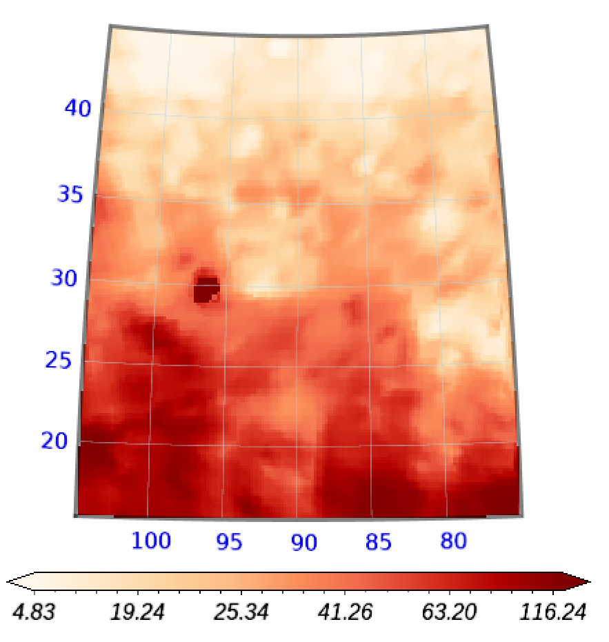
Figure 9: WHAM H$\alpha$ wide image, in Galactic coordinates, of the sky centered on HD 163466 (located at $l=89^{\circ}.24$, $b=30^{\circ}.56$). The horizontal “thermometer” is EM (${\rm cm^{-3}\,pc}$) scaled up by a factor of 22. In the direction towards HD 163466 (marked by a circle) the emission measure is about $1\,{\rm cm^{-6}\,pc}$. The bright emission region at $l\approx 95^{\circ}$ and $b\approx 30^{\circ}$ is NGC 6543. Figure provided by M. Haffner.

5 Inference

The [NeII] 12.814 $\mu$m photon intensity of $15.2\pm 2\,R$ (see Table 4) can, using Equation 1, be used to infer the EM, subject only to our assumption of temperature, $T$ of 8,000 K and adopted gas-phase abundance of neon. We make little error in assuming $x_{\rm H^{+}}=1$. With that simplification the emission measure is $8.2x_{\rm Ne^{+}}^{-1}$. Even if $x_{\rm Ne^{+}}$ is as low as 0.5 the inferred emission measure is modest, ${\rm 16\,cm^{-6}\,pc}$. Thus, it is reasonable to assume that [NeII] emission arises in the WIM. In support of this inference we note that the [NeII] emission towards HD 163466, some 1.3^′ away, is at the same level as that measured in the background field direction. From Table 4 we find that the 2-$\sigma$ upper limit is [NeIII]/[NeII]$<1.13$ and is not particularly informative.

One of the four instruments on the Infrared Space Observatory (ISO) was the Short Wave Spectrometer (SWS; 2.4–45 $\mu$m). Giveon et al. (2002) undertook an extensive study of HII regions in a number of mid-IR fine structure lines. They found [NeIII]/[NeII] to vary from 0.1 (at small Galactocentric radii) to unity (at the solar circle and beyond), albeit with significant scatter. For HD 163466 the observed [NeIII]/[NeII] ratio is $0.49\pm 0.32$. Given that we have a single determination and the scatter in the radial dependence of the [NeIII]/[NeII] ratio we are not able to draw any useful conclusion. Next, as can be seen from Figure 10 the [NeIII]/[NeII] intensity ratio is quite insensitive to the temperature of the gas. At the 3-$\sigma$ level we see that, $x_{\rm Ne^{+2}}/x_{\rm Ne^{+}}<0.57$ which means that [NeII] is more abundant than [NeIII] – this is entirely expected in ionization models of the WIM (e.g., Mathis 1986).

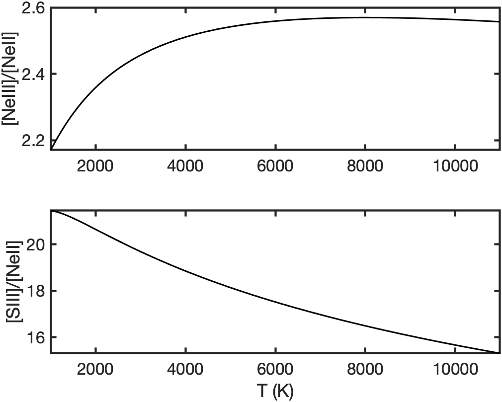
Figure 10: (Top) The run of [NeIII]/[NeII] as a function of temperature. (Bottom) The run of [SIII]/[NeII] as a function of temperature. The multiplicative scale factor is $x_{\rm S^{+2}}/x_{\rm Ne^{+}}$.

In Figure 10 we plot the [SIII]18.71/[NeII]12.81 ratio. The observed ratio is $2.2\pm 0.44$ from which we deduce that $x_{\rm S^{+2}}/x_{\rm Ne^{+}}=0.133\pm 0.027$. To the extent that our adopted abundances are accurate this result points to a significant decrease in the ionizing power of the incident EUV field from 21.6 eV (ionization potential of Ne I; see Table 1) to 23.3 (the ionization potential of S II; ibid).

5.1 H$\alpha$: WHAM

WHAM produced an H$\alpha$ map of the sky at one-degree angular resolution (Haffner et al., 2003). The WHAM H$\alpha$ map centered on HD 163466 is shown in Figure 9. As can be seen from Figure 9 the field of HD 163466 is not dominated by any strong nebula.

From the WHAM catalog we extracted the spectrum closest to the line-of-sight to HD 163466 (see Figure 11). The integrated intensity is $1.14\pm 0.04\,R$. The peak at $v_{\rm LSR}\approx 0$ arises in the local “Orion” spur while the negative velocity emission at, say, $v_{\rm LSR}\approx{\rm-30\,km\,s^{-1}}$ arises in the Perseus arm (see Xu et al. 2016). The intensity weighted mean LSR velocity is $-2\,{\rm km\,s^{-1}}$. The estimated reddening, ${\rm E(B-V)}$, is about 0.05 mag. The corresponding extinction at H$\alpha$ is about 0.1 mag. The extinction corrected value is $1.26\pm 0.04\,R$. Some of the observed H$\alpha$ is due to scattering of brighter Galactic H$\alpha$ by interstellar dust into the line-of-sight. We apply a scattering correction of 15% (Wood & Reynolds, 1999) and find $I_{\rm H\alpha}=1.07\pm 0.03\,R$. For $T=8,000\,$K, the inferred emission measure is $2.4\,{\rm cm^{-6}\,pc}$ significantly smaller than that inferred from observations of [NeII]. Given the widely differing angular scales of MRS and WHAM (cf. §2.3), we are not alarmed by the discrepancy.

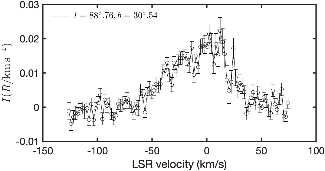
Figure 11: The H$\alpha$ intensity spectrum from the Wisconsin H$\alpha$ Mapper (WHAM). The unit for intensity is $R$ (km s${}^{-1})^{-1}$ while the $x$-axis is the velocity with respect to the local standard of rest (LSR). The spectrum is typical in this region and is usually decomposed into into two Gaussian components: one centered at $v_{\rm LSR}\approx 0\,{\rm km\,s^{-1}}$ for the local (Orion) arm and the other at $\approx-30\,{\rm km\,s^{-1}}$ (Perseus arm).

5.2 [NeII]

The barycentric velocity of the [NeII] line is $-20\pm 12\,{\rm km\,s^{-1}}$ (also Table 8). The corresponding velocity with respect to the Local Standard of Rest (LSR) is $-37\pm 12\,{\rm km\,s^{-1}}$. It appears that the [NeII] emission is associated with negative velocity H$\alpha$ emission which can be traced to the Perseus arm, at a distance of about 5 kpc (see Xu et al. 2016). The vertical scale height is 2.5 kpc. The temperature of the WIM rises with the vertical distance (Haffner et al., 1999; Madsen et al., 2006). It may well be that a better value for the temperature is $10^{4}\,$K – which, for a given EM, would increase [NeII] and [SIII] emission.

H$\alpha$ measurements obtained on angular scales similar to that of MRS, if available, would have allowed us to infer the ionization fraction of Ne⁺ and S⁺⁺. We currently lack this option because the primary source of H$\alpha$ data is WHAM which has one-degree beam. Fortunately, as discussed below (§6.2) modern IFUs on large ground-based optical telescopes will make it possible to measure not only H$\alpha$ but also the full suite of optical nebular lines of interest to WIM studies.

6 Conclusions

MIRI-MRS, as a part of commissioning observed a calibrator star, HD 163466 and an associated “background” field. This intermediate latitude line-of-sight ($l=88^{\circ}.8$, $b=30^{\circ}.5$) does not include any bright nebulae. We obtained the sky spectrum by taking the median of each image slice of the background field data cube. We detected strong [Ne] $12.814\,\mu$m at a barycentric velocity of $-20$ km s^-1, [SIII] 18.713 $\mu$m and possibly [SIV] 10.510 $\mu$m. The photon statistics in the HD 163466 data set are dominated by photons emitted by bright calibrator star. We masked out bright emission from the stars and undertook a similar analysis. [NeII] emission is readily detected while [SIII] is marginally detected. From the neon observations we infer an emission measure, EM$\approx(8.2\pm 1.1)x_{\rm H^{+}}/x_{\rm Ne^{+}}\,{\rm cm^{-3}\,pc}$. The low value of the inferred EM lead us to conclude that these lines arise in the Galactic WIM. We measure $x_{\rm Ne^{+}}/x_{\rm Ne^{++}}<0.6$ and $x_{\rm S^{++}}/x_{\rm Ne^{+}}=0.13\pm 0.027$. These values are consistent with the standard low ionization parameter model for the WIM (Mathis, 1986; Domgörgen & Mathis, 1994; Sembach et al., 2000) On a one-degree scale (as compared to few arcsecond scale of MRS) the inferred EM from ground-based H$\alpha$ emission is $2.4\,{\rm cm^{-3}\,pc}$.

The detection of [NeII] emission on arcsecond scales augers well for the MRS to study tiny ionized nebulae. The radius of the Strömgren sphere is

$$R_{S}=\bigg{(}\frac{3Q_{0}}{4\pi n_{H}^{2}\alpha}\bigg{)}^{1/3}=1.5\times 10^{-2}\,Q_{40}^{1/3}n_{1}^{-2/3}\,{\rm pc}$$

where $n_{\rm H}=10n_{1}\,{\rm cm^{-3}}$ is the H-atom density, $Q_{0}$ is the rate of ionizing photons emitted by the star and $Q_{40}=Q_{0}/10^{40}\,{\rm photon\,s^{-1}}$. The corresponding emission measure is ${\rm EM}=1.94n_{1}^{4/3}Q_{40}^{1/3}\,{\rm cm^{-6}\,pc}$. The ionizing photon luminosity of a white dwarf (radius, $R=0.014\,R_{\odot}$) at a temperature $T=[1.7\times 10^{4},1.0\times 10^{4}]\,$K is $[2.9\times 10^{40},2.8\times 10^{37}]\,{\rm s^{-1}}$. So a white dwarf embedded in the Warm Neutral Medium (volume filling factor of over a third; $n_{\rm H}\approx 1\,{\rm cm^{-3}}$) or an A star embedded in the Cold Neutral Medium (filling factor less than a percent; $n_{\rm H}\approx 30\,{\rm cm^{-3}}$) will have nebulae that are detectable by MRS. Both nebulae lack sharp Strömgren spheres.

6.1 A JWST Comensal Program

The results presented here are limited by uncorrected fringing and not fully calibrated spectral baselines. The current state of affairs is not surprising. IFUs are powerful but are also complex instruments. Past experience has shown that it will take effort and time to calibrate IFUs. We will assume that in due course the MIRI-MRS pipeline will routinely produce photon-noise limited data cubes and the sensitivities summarized in Table 2 will be achieved.

The median WIM H$\alpha$ emission for $|b|>20^{\circ}$ is $1\,R$ which corresponds to an emission measure of $2.2\,{\rm cm^{-3}\,pc}$. Several large regions of low-latitude sky (e.g., Perseus arm, $l=130^{\circ},b=-7.5^{\circ}$; see Madsen et al. 2006) have bright WIM emission, $I_{\rm H\alpha}\approx 10\,R$. Table 2 shows that with an hour long integration MIRI-MRS has the capability to detect [NeII], [ArII], [SIII] and perhaps even [SIV] from a good fraction of the sky, both at high latitude and most certainly at intermediate and low latitude.

Thus, over the course of the lifetime of JWST, we can expect suitable MRS data sets to grow steadily. This is a fine example of highly productive “comensal” observing by JWST. The increasing sample will give astronomers statistical power to explore the variations in the spectrum of the diffuse EUV radiation field and, in due course, measure the volume filling factor of the Warm Neutral Medium (WNM).

6.2 Joint studies with ground-based IFUs

Ground-based optical facilities are well suited to studies via nebular lines as well as hydrogen and helium recombination line studies. Over the last decade, high spectral resolution IFU spectrographs have been commissioned on large ground-based optical telescopes (e.g, MUSE/VLT, Bacon et al. 2014; KCWI/Keck, Morrissey et al. 2018).

The sky background, on a moonless and clear night, at Paranal (Jones et al., 2013) or Mauna Kea is about $200\,{\rm photon\,m^{-2}\,\mu{m}^{-1}\,arcsec^{-2}}$ for for $\lambda<0.7\mu$m which corresponds to about $1.1\,R$ Å^-1. The background gradually rises to ten times this value as one proceeds to 1 $\mu$m. For some lines, air glow line emission will dominate over the continuum background. Geo-coronal H$\alpha$ emission is 2–4 $R$ even at mid-night (Nossal et al., 2008). [NI] and [OI] lines are both very strong (up to 30 $R$ for [NI] and up to 200 $R$ for [OI]) and variable. The air glow lines will be at zero topocentric velocities while the velocity of the astronomical signal will include the projected component of earth’s orbital velocity. Thus, for some lines of sight, with some planning, the air glow contribution can be reduced.

Let $\mathcal{B}$ be the sky brightness in unit of Rayleigh per Angstrom and $\mathcal{S}$ be the photon intensity of the line of interest, also in Rayleigh. We adopt 1 Å as the default spectral channel width, $\Delta\lambda$ and separately note that at the wavelength of H$\alpha$, for instance, 1 Å corresponds to 45 km s^-1. The signal-to-noise ratio (SNR) for an IFU with field-of-view of $\Omega$ operating in a light bucket mode is

$${\rm SNR}=\frac{\eta\alpha\mathcal{S}A\Omega t}{(\eta\alpha\mathcal{B}A\Omega t\Delta\lambda)^{1/2}}$$ (3)

where $\alpha=10^{6}/(4\pi)$ is the conversion factor between intensity in Rayleigh to photon intensity and the other symbols have the same meaning as in Equation 2.

An illustrative example is the Keck Cosmic Imager. At the highest spectral resolution, the input aperture is $\Omega=20^{\prime\prime}\times 8.2^{\prime\prime}$. We simplify by setting $\eta=0.15$ and $\mathcal{R}=15,000$ for the entire optical range. The spectral FWHM would then vary from 0.2 Å at the blue end to 0.6 Å at the red end. The signal-to-noise ratio (SNR) is

$${\rm SNR}=361\bigg{(}\frac{\mathcal{S}}{\sqrt{\mathcal{B}}}\bigg{)}\Big{(}\frac{\eta}{0.15}\Big{)}^{1/2}\Big{(}\frac{\Delta\lambda}{1\,\textrm{\AA}}\Big{)}^{-1/2}t_{\rm hr}^{1/2}{\rm EM}$$ (4)

where $t_{\rm hr}$ is the integration time in hours. H$\alpha$ data, when combined with JWST [NeII] detection, will make it possible to deduce ionization fraction of Ne⁺. Furthermore, this SNR is so high that useful images can be constructed with 1-arcsecond pixels. Thus, ionized nebulae can be probed on arc-second scales!

Next, consider sulfur and neon. The optical nebular lines are temperature sensitive. The sky spectrum in the vicinity of [SIII] $\lambda$9531 Å line is shown in Figure 12. The expected SNR for this line $304\xi_{\rm S^{+}2}/x_{\rm H^{+}}t_{\rm hr}^{1/2}{\rm EM}$. The SNR for [NeIII] $\lambda$3869 Å is $90\xi_{\rm Ne^{+}2}/x_{\rm H^{+}}t_{\rm hr}^{1/2}{\rm EM}$. Joint analysis of the optical and MIRI-MRS data will yield the temperature of the WIM. In addition, the traditional optical forbidden lines (e.g., [OII], [OIII], [NII], [SII] etc) can be observed with KCI and thereby obtain a comprehensive view of the ionization of the WIM. Inversely, the large SNRs for many optical lines mean that every deep KCI observation is comensal – with every deep high spectral resolution observation leading to detections of the WIM.

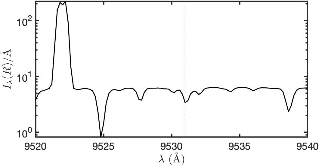
Figure 12: The spectrum of the sky in the vicinity of the [SIII] 9531 Å line (marked vertical dotted line), as observed at the Gemini Observatory atop Mauna Kea.

6.3 Helium Recombination Lines

Pinning down the ionization fraction of helium in the WIM is a long standing goal. The two strongest recombination lines are 5865 Å line and 1.083 $\mu$m. Benjamin et al. (1999) provide volume emissivity for various helium recombination lines. These emissivities are referenced to the emissivity of the He I $\lambda$ 4471 Å ($1s4d\,^{3}{\rm D}\rightarrow 1s2p\,^{3}{\rm P}^{o}$ line. We find the volume emissivities for HeI $\lambda$1.083 $\mu$m triplet ($1s2p\,^{3}{\rm P}^{o}\rightarrow 1s2s\,^{3}{\rm S}$) and HeI $\lambda$5875 Å ($1s3d\,^{3}{\rm D}\rightarrow 1s2s\,^{3}{\rm S}$) to be the following:

$$4\pi n_{5875} = 5.0\times 10^{-14}T_{4}^{-1.065}n_{e}n_{\rm H^{+}}\,{\rm cm^{3}\,s^{-1}}$$

$$4\pi n_{1.083} = 1.9\times 10^{-13}T_{4}^{-0.523}n_{e}n_{\rm H^{+}}\,{\rm cm^{3}\,s^{-1}}$$

where $\dot{n}_{\lambda}=j_{\nu}/(h\nu)$ with $j_{\nu}$ being the emissivity. The corresponding photon intensity along a line-of-sight is

$$I_{5875} = 1.26\times 10^{-2}\xi_{\rm He^{+}}T_{4}^{-1.065}\,{\rm EM}\,R\ ,$$

$$I_{1.083} = 4.8\times 10^{-2}\xi_{\rm He^{+}}T_{4}^{-0.524}\,{\rm EM}\,R\ .$$

A few observations were undertaken with WHAM in HeI $\lambda$5875 (Reynolds & Tufte, 1995). Here, we explore the detectability of the latter with NIRSpec/JWST operating in the IFU mode (Böker et al., 2022; Jakobsen et al., 2022).

For the IFU we assume an entrance aperture, $\Omega=3^{\prime\prime}\times 3^{\prime\prime}$. For HeI 1.083 $\mu$m line the appropriate grating is G140H, $\eta\approx 0.3$ and $\mathcal{R}=2700$ (Giardino et al., 2022). The corresponding background intensity is ${\rm 0.3\,MJy\,ster^{-1}}$. For $T=8,000\,$K the HeI 1.083 $\mu$m intensity is $0.054\xi_{\rm He^{+}}\,{\rm EM}\,R$. The resulting SNR is

$${\rm SNR}=2.5\xi_{\rm He^{+}}\Big{(}\frac{\eta}{0.3}\Big{)}^{1/2}\Big{(}\frac{\mathcal{R}}{2700}\Big{)}^{1/2}\Big{(}\frac{t}{1\,{\rm hr}}\Big{)}^{1/2}\,{\rm EM}\ .$$

Directions with EM of $\gtrsim 10\,{\rm cm^{-6}\,pc}$ are ideal to measure the helium ionization fraction. Over the duration of the mission, stacking of pointings with EM of few ${\rm cm^{-6}\,pc}$ would probe the ionization at high latitude.

Figure 13: The spectrum of the sky as observed at the Gemini Observatory atop Mauna Kea. The wavelengths are measured in air. The black vertical dotted line marks the position of HeI 1.08300 $\mu$m line. The red dotted lines mark OH lines. These are, from left to right, OH 5-2 Q2 (0.5), 5-2 Q1(1.5), 5-2 Q1(2.5); see Rousselot et al. (2000).

How about ground-based facilities? In the vicinity of the 1.083 $\mu$m recombination line the sky continuum intensity is about $5\,R$ Å^-1 (see Figure 13). He atoms in the terrestrial exosphere are excited by energetic electrons to the $1s2p\,^{3}{\rm P}$ meta stable state and these resonantly scatter solar HeI 1.083 $\mu$m photons. The emission decreases as the sun sets. A key requirement is a spectral resolution of better than 1 Å (to avoid contamination by super-strong OH lines; see Figure 13). A spectral resolution of 0.5 Å is even better (to eliminate terrestrial He I emission); thus, $\mathcal{R}\gtrsim 2\times 10^{4}$. Consider the following hypothetical (future) instrument on an 8-m telescope: $\Omega=100\,$arcsec², $\eta=0.3$, $\mathcal{R}=2\times 10^{4}$. The SNR is then $9.7\xi_{\rm He}t_{\rm hr}^{1/2}{\rm EM}$. Thus, such an instrument would be more sensitive than NIRSPEC/JWST. Another possibility is a Fabry-Pérot imager (on a smaller telescope). A different approach is to use optical lines, specifically the $\lambda$5865 line. With KCWI the SNR is $10.4\xi_{\rm He}t_{\rm hr}^{1/2}$.

6.4 Fine Structure in the WIM

At the beginning of this section we noted that the inferred EM from [NeII] is $(8.2\pm 1.1)\xi_{\rm Ne^{+}}^{-1}$. In §5.1 we concluded that the emission measure inferred from the 1-degree WHAM H$\alpha$ sky survey, after correcting for reflection from dust, is ${\rm EM}=2.4\,{\rm cm^{-6}\,pc}$. It appears that the EM at the smaller angular scale of MIRI-MRS (a few arcseconds) is $3.4/\xi_{\rm Ne^{+}}$ larger than that measured on one degree scale. We advance the idea that the WIM has significant fluctuations on sub-degree scales which are smoothed over by the degree-beam of WHAM. If so, in due course, comparison of MIRI-MRS observations with WHAM will provide insight into the fine structure of the WIM.

Appendix A Fine-structure lines

Table 6: Fine-structure lines

ion	$u$–$l$	$\lambda\ (\mu{\rm m})$	$A_{ul}\,({\rm s}^{-1})$	0	$T_{u0}$ (K)	$\Omega_{u0}$
[NeII]	${}^{2}{\rm P}_{\nicefrac{{1}}{{2}}}^{o}$–${}^{2}{\rm P}_{\nicefrac{{3}}{{2}}}^{o}$	12.813548(20)	$8.6\times 10^{-3}$	${}^{2}{\rm P}_{\nicefrac{{3}}{{2}}}^{o}$	1123	$0.314T_{4}^{0.076+0.002{\rm ln}\,T_{4}}$
[NeIII]	${}^{3}{\rm P}_{1}$–${}^{3}{\rm P}_{2}$	15.5551	$5.8\times 10^{-3}$	${}^{3}{\rm P}_{2}$	925	$0.774T_{4}^{0.068-0.0556\,{\rm ln}\,T_{4}}$
[NeIII]	${}^{3}{\rm P}_{0}$–${}^{3}{\rm P}_{1}$	36.0135a	$1.1\times 10^{-3}$	${}^{3}{\rm P}_{2}$	1324	$0.208T_{4}^{0.056-0.053\,{\rm ln}\,T_{4}}$
[ArII]	${}^{2}{\rm P}_{\nicefrac{{1}}{{2}}}^{o}$–${}^{2}{\rm P}_{\nicefrac{{3}}{{2}}}^{o}$	6.985274(4)	$5.3\times 10^{-2}$	${}^{2}{\rm P}_{\nicefrac{{1}}{{2}}}^{o}$	2060	$2.93T_{4}^{0.084-0.014{\rm ln}\,T_{4}}$
[ArIII]	${}^{3}{\rm P}_{1}$–${}^{3}{\rm P}_{2}$	8.99138(12)	$3.1\times 10^{-2}$	${}^{3}{\rm P}_{2}$	1601	$4.04T_{4}^{0.031+0.002{\rm ln}\,T4}$
[ArIII]	${}^{3}{\rm P}_{0}$–${}^{3}{\rm P}_{1}$	21.8302(3)	$5.9\times 10^{-3}$	${}^{3}{\rm P}_{2}$	2259	$1.00T_{4}^{0.111-0.009{\rm ln}T_{4}}$
[SIII]	${}^{3}{\rm P}_{2}$–${}^{3}{\rm P}_{1}$	18.713	$2.6\times 10^{-3}$	${}^{3}{\rm P}_{0}$	1199	$7.87T_{4}^{-0.171-0.033{\rm ln}\,T_{4}}$
[SIV]	${}^{2}{\rm P}_{\nicefrac{{3}}{{2}}}^{o}$–${}^{2}{\rm P}_{\nicefrac{{1}}{{2}}}^{o}$	10.5105	$7.4\times 10^{-3}$	${}^{2}{\rm P}_{\nicefrac{{1}}{{2}}}^{o}$	1369	$8.54T_{4}^{-0.012-0.076{\rm ln}\,T_{4}}$

Note. — The quoted vacuum wavelength is the one with uncertainty of the Ritz or measured values. The uncertainty, shown in the parenthesis, is the last one or two digits of the wavelength value. Column 1 is the species and column 2 is the terms of the transitions (with $l$ for lower state and $u$ for the upper state). The wavelengths (column 3) and A-coefficients (column 4) are from NIST. The column marked with “0” is the term for the ground level. $T_{u0}=E_{u0}/k_{B}$ is the line energy equivalent temperature (column 6); here, $E_{u0}$ is the energy of the upper level $u$ (noted in the first column) with respect to ground level (“$0$”). The collisional strength (last column), $\Omega_{u0}$, is for excitation from level $0$ to level $u$; the data are from Draine (2011). ^aThis line is beyond the reach of the spectrometers of JWST but is include here because excitations to ${}^{3}{\rm P}_{0}$ also result in emission of 15.56 $\mu$m photons.

Appendix B HD 163466

HD 163466 ($\alpha$=17:52:52.37, $\delta$=+60:23:46.9; $l=89^{\circ}.24,b=30^{\circ}.56$) is one of the JWST calibrator stars (Krick et al., 2021). It is listed by Simbad as a bright ($V=6.85$) emission-line star of type A2e. The Gaia parallax is $5.208\pm 0.04\,$mas. At this distance the proper motion amounts to $-1.8\,{\rm km\,s^{-1}}$ in right ascension and 39 km s^-1 along the declination axis. The star with an estimated age of 310 Myr is not a part of any moving group. The radial velocity is $-16\,{\rm km\,s^{-1}}$. HD 163466  was a part of a sample of A stars with debris that was observed with the Spitzer Space Telescope (Su et al., 2006).

Given the newness of the MIRI data we checked its calibration in a number of ways. First to assess the point source photometry we extracted the signal at 12.814 and 15.5505 $\mu$m in a 3″-radius and compared those with observed by the WISE satellite (Wright et al., 2010) and extrapolated using a Rayleigh-Jeans law, $F_{\nu}\propto\nu^{2}$. The agreement is excellent: WISE 0.0676$\pm$0.001 Jy and 0.0459$\pm$0.001 at 12.814 and 15.5505 $\mu$m, respectively vs. MIRI 0.0674$\pm$0.001 Jy and 0.0410$\pm$0.001 Jy with an assumed calibration uncertainty of 2%. These correspond to differences of 2 and 10% at the two wavelengths.

Appendix C NGC 6543

The planetary nebula NGC  6543 was observed during the commissioning of MIRI-MRS (PID#1047 and #1031). The log can be found in Table 7.

Table 7: Summary of log of data sets for NGC  6543

name	$\alpha$ (deg)	$\delta$ (deg)	series	Aperture (″)	$\tau$(s)
NGC6543 ([NeII],[NeIII])	269.63667	66.63133	jw01047-o001_t006	4.0	4129
NGC6543 ([ArII])	269.64313	66.63344	jw01031-c1003_t010	0.7	4129
NGC6543 ([SIII])	269.64313	66.63344	jw01031-o012_t010	2.0	4129

Note. — The “name” refers to our assigned name for the data set. The next two columns are J2000 right ascension and declination, followed by file name identifier of the Level-3 MIRI-MRS pipeline data sets. The next column is the radius of the photometric aperture followed by the integration time.

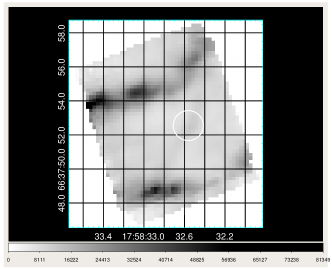
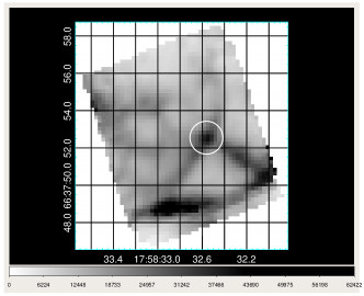
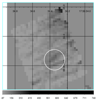
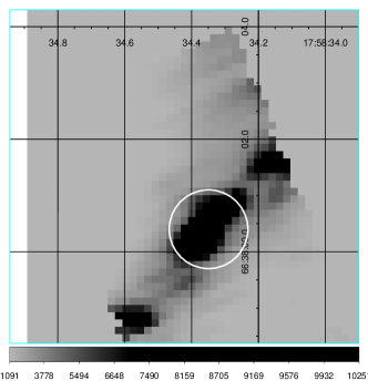
Figure 14: (Top) Location of aperture on knot of [NeII] emission in the Planetary Nebula NGC6543 off and nn the 12.8 $\mu$m line (right and left, respectively. (Bottom ) Emission from the knot in the 6.95 $\mu$m of [ArII] off and on the line

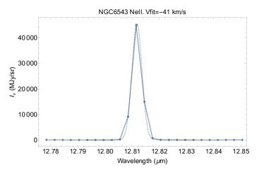
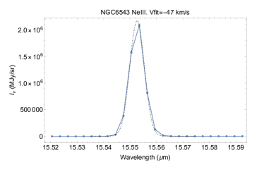
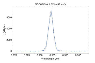
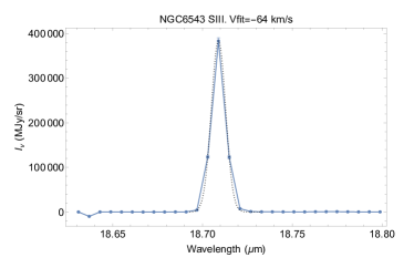
Figure 15: top) Emission from the knot in the 12.8 $\mu$m (right) and 15.55 $\mu$m (left) lines of [NeII] and [NeIII], respectively. bottom) emission in [ArII] and [SIII]. In all cases the emission lines are unresolved. The dotted black lines denote the results of Gaussian fits to the emission with the FHWMs at leach wavelength used in the analysis of the HD 163466 observations.

Table 8: Analysis of NGC 6543

		Ampl	$\lambda$	FWHM	Vfit	Integrated Inten.
Object	Line	MJy $sr^{-1}$	$\mu$m	$\mu$m	km s-1	${\rm erg\,cm^{-2}\,s\,^{-1}\,arcsec^{-2}}$
NGC  6543	[ArII]	(7.120$\pm 0.045)\times 10^{4}$	6.98441	0.00208	$-36.9$	($2.36\pm 0.01)\times 10^{-14}$
NGC  6543	[NeII]	(4.539$\pm 0.008\times 10^{4}$	12.8118	0.00431	$-41.50$	($8.976\pm 0.001)\times 10^{-14}$
NGC  6543	[NeIII]	(2.17$\pm 0.008)\times 10^{6}$	15.5527	0.00649	$-46.63$	$(4.37\pm 0.002)\times 10^{-12}$
NGC  6543	[SIII]	(3.83$\pm 0.002)\times 10^{5}$	18.709	0.00938	$-64\pm 8^{1}$	($7.716\pm 0.004)\times 10^{-13}$

Note. — ¹Velocity uncertainty due to uncertainty in rest wavelength.

Figure 14 shows knots of [NeII] and [ArII] emission taken in slightly different regions of the nebula and measured in and out of the lines. The resultant line intensities are so strong that the data filtering required for the weak lines seen toward HD 163466 was not required. A linear baseline was subtracted from the median values within the given apertures (Table 7) as shown in Figure 15. These data demonstrate the ability of MIRI-MRS to detect robustly the lines of [NeII], [NeIII], [ArII] and [SIII]. Table 8 summarizes the observational data and derived parameters. The intrinsic widths of lines within NGC  6543 are 10 to 15$\,{\rm km\,s^{-1}}$ (Bryce et al., 1992) and are thus unresolved at the $R\sim 2700$ spectral resolution of MRS. We fitted the line profiles with a Gaussian and report the full width at half-maximum (FWHM) in Table 8. As described in Wells et al. (2015), the MRS spectra are under sampled which accounts for the narrowness of the spectra presented in Figure 15.

Table 8 gives resultant heliocentric velocities for the different lines ranging from $-40$ to $-68\,{\rm km\,s^{-1}}$. Although the systemic velocity of NGC  6543 is about $-68\,{\rm km\,s^{-1}}$, observations of [OIII] at 5007$\AA$ averaged over slit lengths of 66–129″(Bryce et al., 1992) showed significant velocity structure from one knot to another suggesting internal motions of a few tens of ${\rm km\,s^{-1}}$. In particular, the region called “A3” (Bryce et al., 1992) close to the site of the MRS observations, shows velocities as low as $-50\,{\rm km\,s^{-1}}$ (Mitchell et al., 2005). Finally, we compared MIRI spectra of NGC6543 in the NeII and NeIII lines obtained with the Spitzer IRS spectrometer. While the spectral resolution is quite different ($\mathcal{R}$=600 vs 2700) and the positions in the nebula different by up to an arc-minute, the agreement between the two spectra is within a factor of two.

References

- Bacon et al. (2014) Bacon, R., Vernet, J., Borisova, E., et al. 2014, The Messenger, 157, 13
- Benjamin et al. (1999) Benjamin, R. A., Skillman, E. D., & Smits, D. P. 1999, ApJ, 514, 307, doi: 10.1086/306923
- Böker et al. (2022) Böker, T., Arribas, S., Lützgendorf, N., et al. 2022, A&A, 661, A82, doi: 10.1051/0004-6361/202142589
- Bryce et al. (1992) Bryce, M., Meaburn, J., Walsh, J. R., & Clegg, R. E. S. 1992, MNRAS, 254, 477, doi: 10.1093/mnras/254.3.477
- Domgörgen & Mathis (1994) Domgörgen, H., & Mathis, J. S. 1994, ApJ, 428, 647, doi: 10.1086/174275
- Draine (2011) Draine, B. T. 2011, Physics of the Interstellar and Intergalactic Medium (Princeton University Press)
- Giardino et al. (2022) Giardino, G., Bhatawdekar, R., Birkmann, S. M., et al. 2022, arXiv e-prints, arXiv:2208.04876. https://arxiv.org/abs/2208.04876
- Giveon et al. (2002) Giveon, U., Sternberg, A., Lutz, D., Feuchtgruber, H., & Pauldrach, A. W. A. 2002, ApJ, 566, 880, doi: 10.1086/338125
- Haffner et al. (1999) Haffner, L. M., Reynolds, R. J., & Tufte, S. L. 1999, ApJ, 523, 223, doi: 10.1086/307734
- Haffner et al. (2003) Haffner, L. M., Reynolds, R. J., Tufte, S. L., et al. 2003, ApJS, 149, 405, doi: 10.1086/378850
- Haffner et al. (2009) Haffner, L. M., Dettmar, R. J., Beckman, J. E., et al. 2009, Reviews of Modern Physics, 81, 969, doi: 10.1103/RevModPhys.81.969
- Hausen et al. (2002) Hausen, N. R., Reynolds, R. J., & Haffner, L. M. 2002, AJ, 124, 3336, doi: 10.1086/344603
- Heiles et al. (1996) Heiles, C., Koo, B.-C., Levenson, N. A., & Reach, W. T. 1996, ApJ, 462, 326, doi: 10.1086/177154
- Jakobsen et al. (2022) Jakobsen, P., Ferruit, P., Alves de Oliveira, C., et al. 2022, A&A, 661, A80, doi: 10.1051/0004-6361/202142663
- Jones et al. (2013) Jones, A., Noll, S., Kausch, W., Szyszka, C., & Kimeswenger, S. 2013, A&A, 560, A91, doi: 10.1051/0004-6361/201322433
- Krick et al. (2021) Krick, J. E., Lowrance, P., Carey, S., et al. 2021, AJ, 161, 177, doi: 10.3847/1538-3881/abe390
- Labiano et al. (2021) Labiano, A., Argyriou, I., Álvarez-Márquez, J., et al. 2021, A&A, 656, A57, doi: 10.1051/0004-6361/202140614
- Madsen & Reynolds (2005) Madsen, G. J., & Reynolds, R. J. 2005, ApJ, 630, 925, doi: 10.1086/432043
- Madsen et al. (2006) Madsen, G. J., Reynolds, R. J., & Haffner, L. M. 2006, ApJ, 652, 401, doi: 10.1086/508441
- Mathis (1986) Mathis, J. S. 1986, ApJ, 301, 423, doi: 10.1086/163910
- Mierkiewicz et al. (2006) Mierkiewicz, E. J., Reynolds, R. J., Roesler, F. L., Harlander, J. M., & Jaehnig, K. P. 2006, ApJ, 650, L63, doi: 10.1086/508745
- Mitchell et al. (2005) Mitchell, D. L., Bryce, M., Meaburn, J., et al. 2005, MNRAS, 362, 1286, doi: 10.1111/j.1365-2966.2005.09399.x
- Morrissey et al. (2018) Morrissey, P., Matuszewski, M., Martin, D. C., et al. 2018, ApJ, 864, 93, doi: 10.3847/1538-4357/aad597
- Nossal et al. (2008) Nossal, S. M., Mierkiewicz, E. J., Roesler, F. L., et al. 2008, Journal of Geophysical Research (Space Physics), 113, A11307, doi: 10.1029/2008JA013380
- Ressler et al. (2015) Ressler, M. E., Sukhatme, K. G., Franklin, B. R., et al. 2015, PASP, 127, 675, doi: 10.1086/682258
- Reynolds (1984) Reynolds, R. J. 1984, ApJ, 282, 191, doi: 10.1086/162190
- Reynolds (1985) —. 1985, ApJ, 298, L27, doi: 10.1086/184560
- Reynolds et al. (2004) Reynolds, R. J., Haffner, L. M., Madsen, G. J., & Tufte, S. L. 2004, in Astronomical Society of the Pacific Conference Series, Vol. 317, Milky Way Surveys: The Structure and Evolution of our Galaxy, ed. D. Clemens, R. Shah, & T. Brainerd, 186
- Reynolds et al. (1977) Reynolds, R. J., Roesler, F. L., & Scherb, F. 1977, ApJ, 211, 115, doi: 10.1086/154908
- Reynolds & Tufte (1995) Reynolds, R. J., & Tufte, S. L. 1995, ApJ, 439, L17, doi: 10.1086/187734
- Reynolds et al. (1998) Reynolds, R. J., Tufte, S. L., Haffner, L. M., Jaehnig, K., & Percival, J. W. 1998, PASA, 15, 14, doi: 10.1071/AS98014
- Rousselot et al. (2000) Rousselot, P., Lidman, C., Cuby, J. G., Moreels, G., & Monnet, G. 2000, A&A, 354, 1134
- Sembach et al. (2000) Sembach, K. R., Howk, J. C., Ryans, R. S. I., & Keenan, F. P. 2000, ApJ, 528, 310, doi: 10.1086/308173
- Su et al. (2006) Su, K. Y. L., Rieke, G. H., Stansberry, J. A., et al. 2006, ApJ, 653, 675, doi: 10.1086/508649
- Tufte (1997) Tufte, S. L. 1997, PhD thesis, University of Wisconsin, Madison
- Wells et al. (2015) Wells, M., Pel, J. W., Glasse, A., et al. 2015, PASP, 127, 646, doi: 10.1086/682281
- Wood & Reynolds (1999) Wood, K., & Reynolds, R. J. 1999, ApJ, 525, 799, doi: 10.1086/307939
- Wright et al. (2010) Wright, E. L., Eisenhardt, P. R. M., Mainzer, A. K., et al. 2010, AJ, 140, 1868, doi: 10.1088/0004-6256/140/6/1868
- Xu et al. (2016) Xu, Y., Reid, M., Dame, T., et al. 2016, Science Advances, 2, e1600878, doi: 10.1126/sciadv.1600878