Quantum geometry beyond projective single bands

Abstract

The past few years have seen a revived interest in quantum geometrical characterizations of band structures due to the rapid development of topological insulators and semi-metals. Although the metric tensor has been connected to many geometrical concepts for single bands, the exploration of these concepts to a multi-band paradigm still promises a new field of interest. Formally, multi-band systems, featuring in particular degeneracies, have been related to projective spaces, explaining also the success of relating quantum geometrical aspects of flat band systems, albeit usually in the single band picture. Here, we propose a different route involving Plücker embeddings to represent arbitrary classifying spaces, being the essential objects that encode $all$ the relevant topology. This paradigm allows for the quantification of geometrical quantities directly in readily manageable vector spaces that a priori do not involve projectors or the need of flat band conditions. As a result, our findings are shown to pave the way for identifying new geometrical objects and defining metrics in arbitrary multi-band systems, especially beyond the single flatband limit, promising a versatile tool that can be applied in contexts that range from response theories to finding quantum volumes and bounds on superfluid densities as well as possible quantum computations.

Introduction. The past decade has witnessed an ever increasing interest in topological matter. Topological insulators and semi-metals provide Qi and Zhang (2011); Hasan and Kane (2010); Armitage et al. (2018) in this regard a direct route to mimic intrinsic topological features and, owing to the inclusion of (crystalline) symmetries, a broad range of results have been achieved Fu (2011); Slager et al. (2012); Kruthoff et al. (2017); Po et al. (2017); Bradlyn et al. (2017); Slager (2019); Scheurer and Slager (2020); Schrunk et al. (2022); Rhim et al. (2018); Kitaev (2009); Schnyder et al. (2008); Song et al. (2018); Bouhon et al. (2021); Elcoro et al. (2021); Watanabe et al. (2018); Kemp et al. (2022); Volovik and Mineev (2018); Van Mechelen et al. (2022); Chiu et al. (2016). While on a case by case bases the synergy between topology and geometry has been rather well established, the past years have seen a reinvigorated interest in the geometrical side. Notably, following the earlier construction of quantum geometric tensors Provost and Vallee (1980); Resta (2011), with a distance measuring real part and imaginary part that encapsulates generalized Berry phases, this object has been in particular useful in the context of topological band theory. Examples include probing single band invariants, such as Chern numbers, in which circularly-polarized light couples to the right elements of the metric tensor to render a response proportional to the determining invariant Ozawa and Goldman (2018); Tran et al. (2017); Salerno et al. (2020); de Juan et al. (2017); Mera and Ozawa (2021); Palumbo (2021) and recent relations with quantum metrology Yu et al. (2022); Li et al. (2022). The latter is particularly appealing in the context of quantum simulators and quenched systems and can even be related to e.g. Cramér-Rao information bounds. In addition, given the surge of interest in flatband physics, notably in the context of twisted multi-layered Van der Waals systems, also relations that bound the superfluid density by general correspondences to the Fubini-Study metric at zero temperature have been receiving increasing interest as well as recent pursuits that relate this density to Wannier properties and real space invariants Peotta and Törmä (2015); Törmä et al. (2021); Begholtz and Liu (2013); Rhim et al. (2020); Herzog-Arbeitman et al. (2022); Parker et al. (2021); Julku et al. (2016); Peri et al. (2021).

In view of all these physical implications a general multi-band approach promises a widely applicable and powerful tool. This relevance is not in the least place also motivated by recent progress on the topological side where recent studies have shown the existence of multi-gap dependent topological phases that culminate in new invariants, such as Euler class Bouhon et al. (2020a); Ahn et al. (2019a); Bouhon et al. (2020b). Multi-gap topologies have been seen in several meta-material studies Jiang et al. (2021a); Guo et al. (2021); Jiang et al. (2022, 2021b); Zhao et al. (2022); Park et al. (2021), and the proposed unusual quench dynamical behavior of Euler class phases Ünal et al. (2020) has been observed in trapped ion insulators Zhao et al. (2022). Similarly, recent proposals in phonon bands and electronic structures under strain have shown to provide feasible routes towards real materials Peng et al. (2022a); Könye et al. (2021); Bouhon et al. (2023a); Peng et al. (2022b); Lange et al. (2021, 2022) and novel anomalous phases Slager et al. (2022).

While there has been recent progress on multi-gap geometrical characterizations, such as the observation that general dipole transitions can be seen as tangent vectors of a Riemannian manifold Ahn et al. (2021), we here point out a general explicit route towards formulating geometric aspects of multi-band systems. Similarly, our approach has no inherent redundancy that comes from taking a specific basis of eigenstates that can be relabeled and thus impose a huge gauge degree of freedom as inherent to recent other setups Ma et al. (2010). Namely, our construction thrives on the key insight that one can directly use the classifying space, the minimal manifold that encodes all topological information without redundant degrees of freedom , and specific characterizations, going by the name of Plücker embeddings, to formulate a general approach to geometric signatures. A Plücker embedding, in essence, is a mapping from a Grassmannian or Flag manifold, which will be shown underneath to be the effective objects to define topology for multi-band settings, into a higher dimensional vector space. We have already shown in recent work Bouhon et al. (2020b); Bouhon and Slager (2022) that Plücker mappings can be employed to define arbitrary multi-gap topological models. Here, however, we take full profit from the geometrical power of this approach that allows for a characterization in terms of straightforward vector spaces. Indeed, as these vector spaces come with very natural geometrical identifications, these embeddings provide for a direct and universal route to define geometrical tensors and properties, providing opportunity to generalize the above mentioned physical impact of the single-band metric to the multi-band context.

This paper proceeds as follows. First we review the single-band metric in the case of band systems having Chern numbers. This provides a good starting point to introduce the Plücker formalism and address the true generalization of single band geometrical notions to a multi-band context, notably in the Chern number context. We then outline how these characterizations offer new routes to model arbitrary topologies, the content of which is then concretely analyzed from a Riemannaian geometrical perspective. We finally highlight the tractable nature of our framework by addressing recently discovered multi-gap topologies in specific models that necessitate descriptions that go beyond single-band formulations and even showcase various general applications that pave the way for future pursuits that will eminently profit from our general perspective.

I Review of single band metric and Chern number

To set the stage we first recall the single band metric formalism in the case of Chern bands. Each band can be viewed as a submanifold of the projective Hilbert space $\mathbb{C}\mathbb{P}^{N-1}$, which is the complex space $\mathbb{C}^{N}$ where all vectors related by complex scalar multiplication are identified. We will use $\left|\tilde{u}\right\rangle$ to denote a vector in $\mathbb{C}\mathbb{P}^{N-1}$ and $\left|u\right\rangle$ to denote a normalized but gauge-dependent representative in $\mathbb{C}^{N}$. This manifold of quantum states is parametrized by crystal momentum $k$, thus assigning a state $\left|\tilde{u}(k)\right\rangle\in\mathbb{C}\mathbb{P}^{N-1}$ to each point of the Brillouin zone. On this manifold one may define a natural metric $g_{ij}$ and symplectic form $\omega_{ij}$,

$$g_{ij} = \mathinner{\langle{\partial_{i}\tilde{u}}|{\partial_{j}\tilde{u}}\rangle}+c.c.$$

$$\omega_{ij} = \mathinner{\langle{\partial_{i}\tilde{u}}|{\partial_{j}\tilde{u}}\rangle}-c.c$$ (1)

The tangent space of $\mathbb{C}\mathbb{P}^{N-1}$ at a point $\left|\tilde{u}\right\rangle$ differs from that of $\mathbb{C}^{N}$ at $\left|u\right\rangle$ by the absence of a vector along $\left|u\right\rangle$ due to the identification of all complex multiples of $\left|u\right\rangle$, so we can write these quantities for a representative $\left|u\right\rangle\in\mathbb{C}^{N}$ by subtracting this component. Defining $Q=\mathbb{1}-\left|u\right\rangle\left\langle u\right|$ as the projector into the tangent space of $\mathbb{C}\mathbb{P}^{N-1}$, we then obtain

$$g_{ij} = \left\langle\partial_{i}u\right|Q\left|\partial_{j}u\right\rangle+c.c.$$

$$\omega_{ij} = \left\langle\partial_{i}u\right|Q\left|\partial_{j}u\right\rangle-c.c.$$ (2)

These form the symmetric and anti-symmetric components of the Fubini-Study metric, respectively. Both the Berry curvature $\omega$ and the quantum metric $g$ describe geometric features of the band with far-reaching consequences on electronic behavior that we have already alluded to above. Indeed, examples include bounds on superfluidity, optical responses when light couples to the right elements to render a response proportional to the Chern number and quantum metrology setups.

When considered from a more mathematical perspective, the curvature $\omega$ has a further description in terms of a connection on $\mathbb{C}^{N}$ viewed as a principle $U(1)$-bundle. A principle $G$-bundle consists of a total space, in this case $\mathbb{C}^{N}$, a projection map $\pi$ to a base space $\mathbb{C}\mathbb{P}^{N-1}$, and a group $G$ acting on the total space, here $U(1)$ by scalar multiplication. Further requirements are that the pre-image of each neighborhood $U$ in the base space is diffeomorphic to $U\times G$, and the group action translates purely within the $G$ component of this trivialization. A connection $A$ is a Lie algebra-valued one-form that maps vertical tangent vectors, those which translate purely within the fiber $G$, to their corresponding element of the Lie algebra. The kernel of $A$ then defines the horizontal section of the tangent space, i.e. vectors that translate purely along base space. In the case of our $U(1)$ bundle, we have the Berry connection

$$A=\mathinner{\langle{u}|{\partial_{i}u}\rangle}$$ (3)

This indeed gives the component of the tangent vector $\left|\partial_{i}u\right\rangle\in T\mathbb{C}^{N}$ along the $U(1)$ fiber, defining an element of the one-dimensional Lie algebra. The Berry curvature is the exterior derivative $\omega=\mathrm{d}A$ of this connection. It is a purely horizontal two-form, describing features of the gauge-invariant base space. Integrating this curvature form then renders the first Chern number associated with the U(1) bundle.

II Multi-band setup and the fundamental role of Grassmannians and Flag manifolds as classifying spaces

A general extension of the above framework to multiple bands necessitates a promotion of these scalar geometric quantities to matrices. If we let $U$ be a matrix whose columns are orthonormal $\left|u\right\rangle$ spanning an occupied collection of bands, we can define

$${\bf g}_{ij} = \partial_{i}U^{\dagger}Q\partial_{j}U+H.c.$$

$$\boldsymbol{\omega}_{ij} = \partial_{i}U^{\dagger}Q\partial_{j}U-H.c.,$$ (4)

where $Q$ generalizes to the projector out of the occupied manifold, $Q=\mathbb{1}-UU^{\dagger}$. Similar to how the $\mathbb{C}^{N}$ representation of the single-band case involved a subtraction of gauge-dependent degree of freedom associated with derivatives along $|u\rangle$, here we remove all components lying within the occupied manifold. This corresponds to a $U(k)$ gauge redundancy, where $k$ is the number of occupied bands. We can now define $\tilde{U}$ to be the identification of all $U(k)$ rotations of $U$, and we obtain

$${\bf g}_{ij}=\partial_{i}\tilde{U}^{\dagger}\partial_{j}\tilde{U}+H.c.$$

$$\boldsymbol{\omega}_{ij}=\partial_{i}\tilde{U}^{\dagger}\partial_{j}\tilde{U}-H.c.$$ (5)

The space of $\tilde{U}$ is best expressed by considering a complete orthonormal basis of $N$ states arranged as columns of $U\in U(N)$ with $k$ states designated as the occupied sector and $N-k$ as the unoccupied sector. $\tilde{U}$ then corresponds to such a $U\in U(N)$ under the identification of all $U(k)$ rotations of the occupied sector and all $U(N-k)$ rotations of the unoccupied sector, i.e. $U(N)/(U(k)\times U(N-k))$. This is the definition of the Grassmanian $Gr^{\mathbb{C}}_{k,N}$. As before, we can view this as a principle $G$-bundle. Though it may seem most natural to consider a $U(k)\times U(N-k)$ bundle, we recall that the $U(N-k)$ component of the gauge group was only introduced as a convenience for considering $U(N)$ as the total space. The relevant part of the gauge group for the occupied manifold is $U(k)$. Since the group is a product, we can easily map to a principle $U(k)$-bundle with total space $U(N)/U(N-k)$. The tangent space to $U(N)$ is the space of anti-Hermitian $N\times N$ matrices, and by quotienting out $U(N-k)$ we remove those with components $\mathinner{\langle{u_{n}}|{\partial u_{m}}\rangle}$ for $u_{n}$, $u_{m}$ unoccupied. The vertical section consists of those matrices with only $\mathinner{\langle{u_{n}}|{\partial_{i}u_{m}}\rangle}$ components where $u_{n}$, $u_{m}$ are both occupied. Thus the Lie algebra-valued connection is the anti-Hermitian $k\times k$ matrix with components $A^{nm}=\mathinner{\langle{u_{n}}|{\partial_{i}u_{m}}\rangle}$, that is

$$A=U^{\dagger}\partial_{i}U.$$ (6)

As before, the curvature $\boldsymbol{\omega}$ is the exterior derivative $\mathrm{d}A$. However, the matrix-valued curvature is not invariant under $U(k)$ rotations. To get something invariant, we must construct a scalar. One useful scalar is the trace, which for the Berry curvature gives the sum of the single-band curvatures over bands $\left|u_{\ell}\right\rangle$ in the occupied manifold.

$$\omega_{ij}\equiv\mathrm{Tr}(\boldsymbol{\omega}_{ij})=\sum_{\ell}\left\langle\partial_{i}u_{\ell}\right|Q\left|\partial_{j}u_{\ell}\right\rangle-c.c.$$ (7)

This quantity integrated over the Brillouin zone gives the Chern number of the occupied manifold. The trace of the symmetric part of the Fubini-Study metric defines a metric on the Grassmanian,

$$g_{ij}\equiv\mathrm{Tr}({\bf g}_{ij})=\sum_{\ell}\left\langle\partial_{i}u_{\ell}\right|Q\left|\partial_{j}u_{\ell}\right\rangle+c.c.,$$ (8)

which then defines the usual notion of distance between two collections of states.

We wish to emphasize the principal topological role of the emergent Grassmannian structure as acting classifying space. The topology of a multi-band model is in all generality set by the relevant classifying space, that, heuristically put, arises by flattening the bands (as dispersion does not affect topological properties), partitioning the system (e.g. in a valence and conduction sector, defining the gap about which topology considered) and removing the redundant degrees of freedom (the permutations of bands in the valence or conduction sector). From a K-theory perspective, meaning a classification perspective that is stable under the addition of trivial bands Kruthoff et al. (2017); Chiu et al. (2016), one usually proceeds by analyzing the Clifford algebra extension problem $Cl_{d}\rightarrow Cl_{d+1}$ Schnyder et al. (2008); Kitaev (2009). The set of representations, denoted by ${\cal C}_{q}$ or ${\cal R}_{q}$ for complex and real case respectively, precisely entails the classifying space, being physically speaking all mass terms that can be added without breaking the assumed symmetries of the system. The topological characterization is then obtained by considering the distinct components, or zeroth homotopy group $\pi_{0}(X)$, where $X={\cal C}_{q}$ or $X={\cal R}_{q}$ Kruthoff et al. (2017); Chiu et al. (2016); Kitaev (2009).

From a homotopy perspective, where one is interested in the topological invariants of a $n$-band system, the classifying space plays a similar fundamental role as it determines the homotopy charges of the relevant Bloch Hamiltonian directly Bouhon et al. (2020b). An illustrative example entails a simple 2D two-band system with Hamiltonian $H=\mathbf{d}(\mathbf{k})\cdot\boldsymbol{\sigma}$ in terms of the Pauli matrices $\boldsymbol{\sigma}$. General maps from the Brillouin zone into the Bloch space of gapped Hamiltonians are in this case determined by the classifying space $Gr^{\mathbb{C}}_{1,2}=U(2)/(U(1)\times U(1)$), being the protective space $\mathbb{CP}^{1}$ or the Riemann sphere. The second homotopy group $\pi_{2}(\mathbb{CP}^{1})=\mathbb{Z}$ then coincides with the opposite Chern number ${\cal C}$ of each band that can take integer values. This is usually rephrased as a ’wrapping of the sphere’ by the $\mathbf{d}(\mathbf{k})$-vector, as quantified using the skyrmion formula ${\cal C}=\frac{1}{4\pi}\int\hat{\mathbf{d}}(\mathbf{k})\cdot\partial_{k_{x}}\hat{\mathbf{d}}(\mathbf{k})\times\partial_{k_{y}}\hat{\mathbf{d}}(\mathbf{k})$ in terms of $\hat{\mathbf{d}}(\mathbf{k})=\mathbf{d}(\mathbf{k})/|\mathbf{d}(\mathbf{k})|$. We stress however that the general point of view on the classifying will underpin richer and more general topologies.

Not in the least place one may note that a general handle on arbitrary classifying space is essential to understand and characterize recently discovered multi-gap topologies as will be detailed in the subsequent sections. These phases arise due to more refined gap conditions that generalize Grassmannians to Flag manifolds Bouhon et al. (2020b); Bouhon and Slager (2022). Considering a three-band system, for example, one may conventionally partition the bands as a two-band and single band subspace, that is $2+1$, or more esoterically as $1+1+1$. This has direct topological consequences when a reality condition due to the presence of $C_{2}{\cal T}$ (two-fold rotations and time reversal symmetry) or ${\cal PT}$ (inversion and time reversal symmetry) is assumed. Indeed, the partition into two sectors then relates to the real Grassmannian $Gr^{\mathbb{R}}_{2,3}=O(3)/(O(2)\times O(1))$ (or oriented forms thereof that give the same homotopy results Bouhon et al. (2020b)), being the real projective plain $\mathbb{RP}^{2}$, while the ‘full Flag limit’ corresponds to $Fl^{\mathbb{R}}_{1,1,1}=O(3)/(O(1)\times O(1)\times O(1)$). Interestingly, the first homotopy group $\pi_{1}(Fl_{1,1,1})$, conveying the possible charges of band nodes, entails the non-Abelian quaternion group $\mathbb{Q}$ Bouhon et al. (2020a); Wu et al. (2019) akin to how vortices act in certain nematics Alexander et al. (2012); Liu et al. (2016); Volovik and Mineev (2018); Beekman et al. (2017). As a result, braiding band node charges between two bands with other nodes residing between two adjacent bands renders phase factors and may lead to similarly valued band node charges within a single two-band subspace. The resulting obstruction to annihilate these nodes is subsequently characterized by a real analogue of the Chern number, the Euler class, that can defined on patches in the Brillouin that include the nodes of this two-band subspace zone to quantify the stability Bouhon et al. (2020a). From a topological point of view, we thus again see the principal role of the classifying space and the relation between different partitions. Indeed, when the third band is subsequently gapped, as is possible for a double braid Bouhon et al. (2020a); Peng et al. (2022b); Bouhon et al. (2020b), this stability of the Euler class in the isolated nodal two-band subspace is precisely captured by the second homotopy of the gapped $2+1$ system that indeed has $\pi_{2}(\mathbb{RP}^{2})=\mathbb{Z}$. In other words, when considering how a system evolves into a multi-gap topological phase characterized by Euler class, we see that starting from a Flag limit in which non-Abelian nodal charges can be braided, we can eventually end up in a gapped system with classifying space $\mathsf{Gr}^{\mathbb{R}}_{2,3}=\mathbb{R}P^{2}$, whose second homotopy group coincides with the Euler class that quantifies the obstruction to annihilate the nodal charges in the isolated two-band subspace due to the previous braiding process Bouhon et al. (2020a); Ünal et al. (2020); Bouhon et al. (2020b).

III Fubini-Study metric in Plucker embedding

The above outlined role of the classifying space manifestly shows that in order to define a general quantum geometric setup, a universal handle on project manifolds as Grassmannians and Flag manifolds is required. Indeed, a pitfall in naively studying multi-band systems using the matrix-valued connection $A$ is that there is a substantial gauge redundancy which makes it easy to consider quantities which may not be observable. One must be careful when considering band off-diagonal quantities, as these may not have physical relevance. More specifically, in the Chern context, the consideration of a collection of states where one does not wish to make any distinction among bands in the occupied sector should ideally result in the mapping of the $U(k)$ gauge theory to a $U(1)$ gauge theory. Similarly, for the multi-gap topologies as analyzed in the subsequent, one requires a general universal handle that notwithstanding does not include physically meaningless unitary or orthogonal rotations of bands in the partitioned subspaces. An essential insight in this regard is that one can depart from the specific relevant classifying space, being the minimal object that encodes all topology, and employ Plücker embeddings as direct universal scheme to concretely parameterize all quantities of interest. To introduce the Plücker embedding we will first motivate it in the familiar Chern context described above, before profiting from its generalizable nature to any Grassmannian or Flag manifold to come to a fully unverisal framework.

As said above, for the characterization of a Chern number of a $k$-band valence sector, the Plücker embedding allows for direct map from the $U(k)$ gauge theory to a $U(1)$ gauge theory. The Plücker embedding is an embedding of $Gr^{\mathbb{C}}_{k,N}$ into $\mathbb{C}^{d}$ where $d=\binom{N}{k}$. Put differently, within this context we map the matrix $U$ representing $k$ states to a single vector in a $d$-dimensional Hilbert space. This single state vector can then be treated using single-band techniques. The Plücker embedding $\iota$ is defined using the wedge product of vectors, which maps $k$ vectors in $N$ dimensions to a vector in $d=\binom{N}{k}$ dimensions and is fully antisymmetric. Given a basis $e_{1},\ldots,e_{N}$ of the original Hilbert space, we define a new basis $\check{e}_{1},\ldots,\check{e}_{d}$ from the $d$ distinct collections $I_{\ell}$ of $k$ indices $\in 1,\ldots,N$ as

$$\check{e}_{\ell}=\bigwedge_{i\in I_{\ell}}e_{i}$$ (9)

Explicitly, a matrix $U$, with elements $u_{i}^{j}$ labeling the $j$th component of the $i$th state, maps to the vector with components

$$V^{\ell}=\epsilon_{i_{1}\ldots i_{k}}u_{1}^{i_{1}}\ldots u_{k}^{i_{k}}\quad i_{1},\ldots,i_{k}\in I_{\ell},$$ (10)

where $\epsilon$ is the Levi-Civita symbol and repeated indices are assumed to be summed over. This defines an explicit way of calculating $P^{\ell}$, however for analytical purposes it will be more useful to work with the object

$$V=u_{1}\wedge\ldots\wedge u_{k},$$ (11)

representing the groundstate manifold in the Plucker embedding, and also the analog to the energy eigenbasis

$$E_{n}=\bigwedge_{i\in I_{n}}u_{i}.$$ (12)

Important algebraic properties of $V$ are the inner product

$$V_{1}^{\dagger}V_{2}=(u_{1}\wedge\ldots\wedge u_{k})^{\dagger}(v_{1}\wedge\ldots\wedge v_{k})=\det(u_{i}^{\dagger}v_{j})$$ (13)

and the Leibniz rule

$$\partial V=\partial u_{1}\wedge u_{2}\wedge\ldots\wedge u_{k}+\ldots+u_{1}\wedge\ldots\wedge u_{k-1}\wedge\partial u_{k}$$ (14)

Furthermore, using the inner product property, one can show that if $u_{1},\ldots,u_{k}$ are orthonormal, then $V$ is normalized. $V$ additionally inherits a $U(1)$ gauge redundancy from the product of $U(1)$ gauge degrees of freedom on the $u_{i}$.

Using these properties, one can show that, see Appendix A,

$$\left\langle\partial_{i}V\right|Q\left|\partial_{j}V\right\rangle-c.c. = \omega_{ij}$$

$$\left\langle\partial_{i}V\right|Q\left|\partial_{j}V\right\rangle+c.c. = g_{ij},$$ (15)

where $Q$ is now $\mathbb{1}-\left|V\right\rangle\left\langle V\right|$. Thus the natural Fubini-Study metric on the Plücker embedding $\iota(U)$ is exactly the trace of the matrix-valued ${\bf g}$ and $\boldsymbol{\omega}$. Similarly, the connection on this $U(1)$ bundle is

$$\mathinner{\langle{V}|{\partial_{i}V}\rangle}=\mathrm{Tr}{A}$$ (16)

We thus observe that, as anticipated, under the Plücker embedding the multi-band generalization of the metric and Chern number map to the single-band version defined on a new Hilbert space, showing its universal power. Naively, the Plücker map constructs a vector parameterization that is invariant under the gauge degrees of freedom (the permutations in the partitioned band subspaces), meaning that it manifestly paramaterizes the right classifying space in a generic manner, giving direct access to all topological invariants. This becomes even more apparent in $n$-band models, where the interplay between partitioning and emergent topological structures is directly tractable in simple models, providing a further intuitive understanding of the Plücker embedding as detailed in the subsequent two Sections.

IV Multi-band systems modeling through Plücker embedding I: Chern phases

The Plücker embedding of Grasmmannians cannot only used in the characterization of the quantum geometry of Bloch Hamiltonians, but can also be used to define arbitrary topological models involving the associated classifying space directly. We here review the use of the Plücker embedding in the systematic modeling of multi-band topological phases. By removing the redundant gauge degrees of freedom, the embedding in fact determines all relevant variables, called principal angles, that most naturally parametrize the points of the Grassmannian.

In this Section and the next, we treat these characterizations in detail. In particular, we will analyze the (“complex”) two-band and three-band Chern phases here, while the (“real”) Euler and Stiefel-Whitney phases are presented in the next section.

IV.1 Two-band Chern models

As outlined above, the classifying space of gapped two-band complex Hamiltonians is the Riemann sphere $\mathsf{Gr}_{1,2}^{\mathbb{C}}=\mathbb{C}P^{1}\cong\mathbb{S}^{2}$. The corresponding Bloch Hamiltonians take the simple form $H^{\mathbb{C},1+1}(\boldsymbol{k})=\boldsymbol{d}(\boldsymbol{k})\cdot\boldsymbol{\sigma}+d_{0}(\boldsymbol{k})\mathbb{1}_{2}$, where the unit vector $\hat{\boldsymbol{d}}\in\mathbb{S}^{2}$ parametrizes the points of the classifying space and its winding determines the Chern number via ${\cal C}=\frac{1}{4\pi}\int\hat{\mathbf{d}}(\mathbf{k})\cdot\partial_{k_{x}}\hat{\mathbf{d}}(\mathbf{k})\times\partial_{k_{y}}\hat{\mathbf{d}}(\mathbf{k})$ in terms of $\hat{\mathbf{d}}(\mathbf{k})=\mathbf{d}(\mathbf{k})/|\mathbf{d}(\mathbf{k})|$. Alternatively, we can start by defining the matrix of Bloch eigenvectors $U^{B}=(u_{1}\,u_{2})$, i.e. entering in the $1+1$-spectral decomposition of the Bloch Hamiltonian

$$H^{\mathbb{C},1+1}=U^{B}\cdot\text{diag}[E_{1},E_{2}]\cdot U^{B\dagger}\,,$$ (17)

where we assume $E_{1}<E_{2}$, in the form of a generic $\mathsf{U}(2)$ matrix parametrized by 4 angles, i.e. $U^{B}=e^{\,\text{i}\varphi}e^{-\,\text{i}\alpha/2\sigma_{z}}e^{-\,\text{i}\beta/2\sigma_{y}}e^{-\,\text{i}\gamma/2\sigma_{z}}$. Clearly the phase $e^{\,\text{i}\varphi}$ and the diagonal factor $e^{-\,\text{i}\gamma/2\sigma_{z}}$ only act as gauge phases of $u_{1}$ and $u_{2}$. We are thus left with a minimal form

$$U^{B}(\alpha,\beta)=e^{-\,\text{i}\alpha/2\sigma_{z}}e^{-\,\text{i}\beta/2\sigma_{y}}\,,$$ (18)

that is parametrized by the two angles that determine a point of the sphere through $\boldsymbol{d}(\alpha,\beta)=-\epsilon(\cos\alpha\sin\beta,\sin\alpha\sin\beta,\cos\beta)$, for which we have set the energy eigenvalues to $E_{1}=-E_{2}=-\epsilon$. We write occupied eigenvector $u_{1}$ as a reference for the 3-band case treated below,

$$u_{1}(\alpha,\beta)=\left[e^{\,\text{i}\alpha/2}\cos\dfrac{\beta}{2}\,,\,e^{-\,\text{i}\alpha/2}\sin\dfrac{\beta}{2}\right]\,.$$ (19)

IV.2 Three-band Chern phases

While the two-band Chern case entails a paradigmatic model, the universal character of the Plücker embedding allows for a direct generalization of this intuitive understanding to novel arbitrary settings. In this regard, we now turn to the systematic modeling of three-band Chern phases where we assume the presence of two occupied bands and one unoccupied one Kemp et al. (2022). Writing the spectral form,

$$H^{\mathbb{C},2+1}=U^{B}\cdot\text{diag}[E_{1},E_{2},E_{3}]\cdot U^{B\dagger}\,,$$ (20)

where $U^{B}=(u_{1}\,u_{2}\,u_{3})\in\mathsf{U}(3)$ and we have assumed $E_{1}\leq E_{2}<E_{3}$, the classifying space is now the complex projective plane $\mathsf{Gr}_{2,3}^{\mathbb{C}}=\mathsf{U}(3)/[\mathsf{U}(2)\times\mathsf{U}(1)]=\mathsf{SU}(3)/\mathsf{S}[\mathsf{U}(2)\times\mathsf{U}(1)]=\mathbb{C}P^{2}$. This is a four-dimensional manifold that can be parametrized by four principal angles. (We refer here to its real dimension. The complex Grassmannian is also a complex manifold of complex dimension 2.)

Similarly to the two-band case, we start with the matrix of Bloch eigenvectors in the form of a generic $\mathsf{SU}(3)$ matrix, i.e. de Guise et al. (2018)

$$U^{B}=U_{23}(\alpha_{1},\beta_{1},\gamma_{1})\cdot U_{12}(\alpha_{2},\beta_{2},\alpha_{2})\cdot U_{23}(\alpha_{3},\beta_{3},\gamma_{3})\,,$$ (21)

in terms of the $\mathsf{SU}(2)$ block matrices

$$[U_{i\,i+1}(\alpha,\beta,\gamma)]_{kl}=[e^{-\,\text{i}\alpha/2\sigma_{z}}e^{-\,\text{i}\beta/2\sigma_{y}}e^{-\,\text{i}\gamma/2\sigma_{z}}]_{kl}\,,$$ (22)

whenever $k,l\in\{i,i+1\}$ and by the identity, i.e. $[U_{i\,i+1}]_{kl}=\delta_{kl}$, when $k,l\not\in\{i,i+1\}$. Out of the eight variables of this generic form, four are redundant to capture the complex projective plane target. Writing $(e_{1},e_{2},e_{3})$ the basis vectors of the ambient complex vector space $\mathbb{C}^{3}$, we take the wedge product of the two occupied Bloch eigenvectors (the first two columns of $U^{B}$) in the spirit of accounting for redundant permutations of bands in the occupied band subspace and verify that

$$V=u_{1}\wedge u_{2}=\check{\boldsymbol{e}}^{\top}\cdot\left[\begin{array}[]{c}e^{\,\text{i}\alpha_{2}}\cos\beta_{2}/2\\ e^{\,\text{i}(\alpha_{1}+\gamma_{1})/2}\cos\beta_{1}/2\sin\beta_{2}/2\\ e^{\,\text{i}(-\alpha_{1}+\gamma_{1})/2}\sin\beta_{1}/2\sin\beta_{2}/2\end{array}\right]\,.$$ (23)

In the above $\check{\boldsymbol{e}}=(e_{1}\wedge e_{2},e_{1}\wedge e_{3},e_{2}\wedge e_{3})$ is the basis of the exterior power space $\bigwedge^{2}(\mathbb{C}^{3})\cong\mathbb{C}^{3}$. We hence see that the angles $(\alpha_{3},\beta_{3},\gamma_{3})$ in Eq. (21) are redundant. After inspection, it turns out that neither the angle $\gamma_{1}$ plays a role in the topology. This leaves the four angles $(\alpha_{1},\beta_{1},\alpha_{2},\beta_{2})$ that fully parametrize the points of the complex projective plane. The minimal form of the Bloch Hamiltonian for all complex $2+1$-partitioned phases is then obtained as

$$H^{\mathbb{C},2+1} (\alpha_{1},\beta_{1},\alpha_{2},\beta_{2})=U^{B}\cdot\text{diag}[E_{1},E_{2},E_{3}]\cdot U^{B\dagger}\,,$$ (24)

$$H^{\mathbb{C},2+1}_{11} =\dfrac{1}{2}(-1-\cos\beta_{1}-\cos\beta_{2}+\cos\beta_{1}\cos\beta_{2})\,$$

$$H^{\mathbb{C},2+1}_{22} =\dfrac{1}{2}(-1+\cos\beta_{1}-\cos\beta_{2}-\cos\beta_{1}\cos\beta_{2})\,$$

$$H^{\mathbb{C},2+1}_{33} =\cos\beta_{2}\,$$

$$H^{\mathbb{C},2+1}_{12} =-e^{\,\text{i}\alpha_{1}}\sin\beta_{1}(\sin\beta_{2}/2)^{2}\,$$

$$H^{\mathbb{C},2+1}_{13} =e^{\,\text{i}(\alpha_{1}+2\alpha_{2}-\gamma_{1})/2}\sin\beta_{1}/2\sin\beta_{2}\,$$

$$H^{\mathbb{C},2+1}_{12} =-e^{-\,\text{i}(\alpha_{1}-2\alpha_{2}+\gamma_{1})/2}\cos\beta_{1}/2\sin\beta_{2}\,$$

where we have taken the energy eigenvalues $E_{1}=E_{2}=-E_{3}=-1$.

The Chern phases are determined by which 2D region of the complex Grassmannian space is covered by $u_{1}\wedge u_{2}$. We find that all the $2+1$-Chern phases are entirely controlled by the two angles $(\alpha_{2},\beta_{2})$. In particular, by setting $(\alpha_{1},\beta_{1},\gamma_{1})=(0,0,0)$, we obtain the form $\left[e^{\,\text{i}\alpha_{2}}\cos\beta_{2}/2,\sin\beta_{2}/2,0\right]$, which is equivalent to Eq. (19).

We finally recover the Berry curvature form from the Plücker vector $V(\alpha_{1},\beta_{1},\alpha_{2},\beta_{2})=u_{1}\wedge u_{2}$ through

$$\Omega^{B} =-\,\text{i}\left[(\partial_{\alpha_{2}}V^{\dagger})\cdot(\partial_{\beta_{2}}V)-(\partial_{\beta_{2}}V^{\dagger})\cdot(\partial_{\alpha_{2}}V)\right]d\alpha_{2}\wedge\beta_{2}\,,$$ (25)

$$=\dfrac{\sin\beta_{2}}{2}d\alpha_{2}\wedge d\beta_{2}\,,$$

from which we get

$$\mathcal{C}_{\mathbb{S}^{2}}=\dfrac{1}{2\pi}\int_{\mathbb{S}^{2}}\Omega^{B}=1\,,$$ (26)

assuming that the angles $(\alpha_{2},\beta_{2})$ cover a base sphere $\mathbb{S}^{2}$ with $\alpha_{2}\in[0,2\pi)$ the azimuthal and $\beta_{2}\in[0,\pi]$ the polar angles (more precisely, such that the unit vector $\boldsymbol{n}(\alpha_{2},\beta_{2})=(\cos\alpha_{2}\sin\beta_{2},\sin\alpha_{2}\sin\beta_{2},\cos\beta_{2})$ wraps the sphere). The above result confirms that when $\mathbb{S}^{2}$ is covered one time, the Plücker vector $V=u_{1}\wedge u_{2}$ covers a nontrivial two-dimensional sphere-image within the Grassmannian, i.e. the image $V(\mathbb{S}^{2})\subset\iota_{P}(\mathbb{C}P^{2})$ is not null-homotopic (it cannot be continuously shrunk to a point within $\mathbb{C}P^{2}$).

Pulling back to the torus Brillouin zone and allowing multiple wrappings of the sphere-image $V(\mathbb{S}^{2})$, we define the mapping

$$H^{W}:\mathbb{T}^{2}\rightarrow\mathbb{S}^{2}:\boldsymbol{k}\mapsto\boldsymbol{n}(\alpha_{2}(\boldsymbol{k}),\beta_{2}(\boldsymbol{k}))\,,$$ (27a)

with a degree $$W\in\mathbb{Z}$$. It is convenient to split this higher winding map into two steps as

$$H^{W}: \mathbb{T}^{2}\xrightarrow{f_{TS}}\mathbb{S}^{2}_{0}\xrightarrow{f^{W}_{SG}}\mathbb{S}^{2}:$$ (27b)

$$\boldsymbol{k}\mapsto(\phi_{0},\theta_{0})\mapsto(\alpha_{2},\beta_{2})\,,$$

such that, reminding that the degree of a map is the number of times it wraps the target space as one scan through its domain, the first map from the torus to the sphere $f_{TS}$ has degree 1 and the second map from the sphere to the Grassmannian $f^{W}_{SG}$ has degree $W\in\mathbb{Z}$ (in particular $f_{SG}=id$), and the resulting map $H^{W}=f^{W}_{SG}\circ f_{TS}$ has degree $W$. Then, the Chern number is nothing but (via pullbacks)

$$\mathcal{C}_{\mathbb{T}^{2}} =H^{W*}\mathcal{C}_{\mathbb{S}^{2}}=f^{*}_{TS}\left[f^{W*}_{SG}\mathcal{C}_{\mathbb{S}^{2}}\right]$$ (28)

$$=\text{deg}(f_{TS})\text{deg}(f^{W}_{SG})=W\in\mathbb{Z}\,.$$

We conclude that all the $2+1$-Chern phases are realized by the Bloch Hamiltonian $H^{\mathbb{C},2+1}(\boldsymbol{k})$ of Eq. (24) with a Chern number $W$ readily fixed by the winding number of the map $f^{W}_{SG}$ from the sphere to its image within the Grassmannian. (While the above pullback structure may seem like a tedious exercise in the context of the three-band Chern phases, it will lie at the basis of our exposition of generalized metrics for an arbitrary number of bands in Section VI.1.)

There remains the question of whether another choice of a pair of angles among the set of variables $\{\alpha_{1},\beta_{1},\alpha_{2},\beta_{2}\}$ would also lead to non-trivial Chern topology. The answer in fact is negative and can be traced back to the so-called CW structure. Although a full treatment of CW complexes is beyond the scope of the present work, we note that the CW structure of a topological space $X$, say of dimension $m$, corresponds to a decomposition of the space into cells $e^{n}$ of increasing dimensions, such that each cell of a certain dimension $n$ is obtained from the inclusion of an $n$-dimensional disc $\mathbb{D}^{n}$ in $X$, and such that the boundary of the disc, $\partial\mathbb{D}^{n}$, is mapped continuously on the cells of dimensions $l\leq n$. Notably for the evaluation of the Chern topology one may deduce that that the CW complex structure of the complex projective plane contains only one sub-Grassmannian sphere, $\mathbb{S}^{2}\cong\mathbb{C}P^{1}\subset\mathbb{C}P^{2}$, parametrized by the angles $(\alpha_{2},\beta_{2})$ (The CW structure of $\mathbb{C}P^{2}$ comprises of a point, the sphere $\mathbb{C}P^{1}\cong\mathbb{S}^{2}$ and a four-dimensional disc $\mathbb{D}^{4}$ whose $\mathbb{S}^{3}$ boundary is glued on the sphere via the Hopf fibration.) In other words, whenever the Plücker vector $V$ does not fully wrap $\mathbb{C}P^{1}$ within $\mathbb{C}P^{2}$, the topology is necessarily trivial.

We crucially note that the topological invariant is insensitive to the local details of the mapping $H^{W}$ from the torus Brillouin zone to the sphere image within the Grassmannian. On the contrary, we will see that such details do affect the quantum geometry of the Bloch eigenstates. We will revisit this point from a more general perspective in the subsequent.

We discuss in Section V.6 a general procedure to obtain explicit tight-binding Hamiltonians from the Plücker ansatz.

V Multi-band systems modeling through Plücker embedding II: Euler and Stiefel-Whitney phases

We continue our demonstration of systematic modeling of topological phases via the Plücker embedding, now focusing on the other fundamental topological class in 2D, namely the (“real”) Euler and Stiefel-Whitney topology Bouhon et al. (2020a); Jiang et al. (2021b); Ahn and Yang (2019); Ünal et al. (2020); Ahn et al. (2019a). We first review the three-band and four-band Euler phases, and then present the $\mathbb{Z}$ Euler to $\mathbb{Z}_{2}$ Stiefel-Whitney topological reduction within five-band phases. Since Euler topology is only realized in orientable two-band subspaces (corresponding to rank-2 real orientable vector bundles), we briefly review the question of orientability that is controlled by the 1D sub-dimensional topology and is indicated by the $\mathbb{Z}_{2}$ first Stiefel-Whitney class. A systematic treatment of the modeling of 1D non-Abelian multi-gap topology will be reported elsewhere Bouhon et al. (2023b).

While the results in the sections on three-band and four-band Euler phases coincide with results of previous work Bouhon et al. (2020b); Bouhon and Slager (2022) on the homotopy classification of these models, we propose here an alternative Plücker-based derivation of the Bloch Hamiltonians that captures more closely the inclusion relation between Grassmannians of increasing dimensions, i.e. $\mathsf{Gr}_{2,3}^{\mathbb{R}}\hookrightarrow\mathsf{Gr}_{2,4}^{\mathbb{R}}\hookrightarrow\mathsf{Gr}_{2,5}^{\mathbb{R}}$. This turns out to be particularly useful for the construction of the five-band models addressed shortly. We also reveal the common geometric origin of topology in complex Chern and real Euler classes that will be useful in the characterization of the quantum geometry of these phases exposed in Sections VI.1 and VIII.

V.1 Reality condition

Contrary to the Chern class, which, within the crystalline context (i.e. symmetric under discrete translations), does not require any additional symmetry, the Euler and Stiefel-Whitney classes are protected by an anti-unitary symmetry (i.e. including complex conjugation) that squares to $+1$ and leaves the quasi-momentum invariant. A ubiquitous example in electronic crystalline systems is the combination of time-reversal symmetry (TRS) ${\cal T}$ and $\pi$-rotation $C_{2z}$ around the axis perpendicular to the system’s basal plane, i.e. here chosen as $\hat{z}$. TRS acts on spin-$1/2$ Bloch orbital states $|\boldsymbol{\varphi},\boldsymbol{k}\rangle=(|\varphi_{A,\uparrow},\boldsymbol{k}\rangle\,|\varphi_{A,\downarrow},\boldsymbol{k}\rangle\,|\varphi_{B,\uparrow},\boldsymbol{k}\rangle\,|\varphi_{B,\downarrow},\boldsymbol{k}\rangle\,\dots)$, where $\{A,B,\dots\}$ label the electronic orbital and sub-lattice degrees of freedom which are both of bosonic type, as ${}^{{\cal T}}|\boldsymbol{\varphi},\boldsymbol{k}\rangle=|\boldsymbol{\varphi},-\boldsymbol{k}\rangle(U_{T}\otimes-\,\text{i}\sigma_{y})\mathcal{K}$, with $U_{\cal T}$ the unitary part acting on the bosonic degrees of freedom and $\mathcal{K}$ is complex conjugation. Similarly, $C_{2z}$ acts as ${}^{C_{2z}}|\boldsymbol{\varphi},\boldsymbol{k}\rangle=|\boldsymbol{\varphi},C_{2z}\boldsymbol{k}\rangle(U_{2}\otimes-\,\text{i}\sigma_{z})$, such that the combination with TRS gives ${}^{C_{2z}{\cal T}}|\boldsymbol{\varphi},\boldsymbol{k}\rangle=|\boldsymbol{\varphi},-C_{2z}\boldsymbol{k}\rangle(U_{2}U_{{\cal T}}\otimes\,\text{i}\sigma_{x})\mathcal{K}$. We recall that for any basis function formed by the (tensor) product of bosonic factors and an odd number of fermionic factors (here the spin $1/2$), we may infer the properties ${\cal T}^{2}=-1$ implying $U_{\cal T}U_{\cal T}^{*}=\mathbb{1}$, $C_{2z}^{2}=-1$ implying $U_{2}U_{2}=\mathbb{1}$ and $C_{2z}{\cal T}={\cal T}C_{2z}$ implying $U_{\cal T}U_{2}^{*}=U_{2}U_{\cal T}$, that lead to $[C_{2z}{\cal T}]^{2}=+1$ since ${}^{[C_{2z}{\cal T}]^{2}}|\boldsymbol{\varphi},\boldsymbol{k}\rangle=|\boldsymbol{\varphi},-C_{2z}\boldsymbol{k}\rangle(U_{2}U_{{\cal T}}U_{2}^{*}U_{{\cal T}}^{*}\otimes\mathbb{1}_{2})=|\boldsymbol{\varphi},-C_{2z}\boldsymbol{k}\rangle$, where $-C_{2z}\boldsymbol{k}=m_{z}\boldsymbol{k}=\boldsymbol{k}$ whenever $\boldsymbol{k}\cdot\hat{z}=0$. Interestingly, spinless TRS combined with spinless $C_{2z}$ also gives $[{\cal T}C_{2z}]^{2}=+1$, leaving basal momenta similarly invariant as in the case of spinless ${\cal PT}$ symmetry (with ${\cal P}$ inversion), such that crystalline bosonic systems are also subjected to Euler and Stiefel-Whitney topological classes. In order to concretize ideas and models, we only refer to the $C_{2}T$ symmetry in the following and take $\boldsymbol{k}$ within the $C_{2}T$-invariant plane.

Writing a Bloch Hamiltonian in the general basis $|\boldsymbol{\varphi},\boldsymbol{k}\rangle$

$$\mathcal{H}=\sum\limits_{\boldsymbol{k}}|\boldsymbol{\varphi},\boldsymbol{k}\rangle H(\boldsymbol{k})\langle\boldsymbol{\varphi},\boldsymbol{k}|\,,$$ (29)

and defining $U_{2{\cal T}}=U_{2}U_{\cal T}$, the condition of $C_{2}{\cal T}$ symmetry ${}^{C_{2z}{\cal T}}\mathcal{H}=\mathcal{H}$ leads to the constraint

$$U_{2{\cal T}}\cdot H(\boldsymbol{k})^{*}\cdot U_{2{\cal T}}^{\dagger}=H(\boldsymbol{k})\,.$$ (30)

The condition $[C_{2z}{\cal T}]^{2}=+1$ implies $U_{2{\cal T}}^{\top}=U_{2{\cal T}}$, i.e. it is unitary and symmetric, in which case the Takagi factorization $U_{2{\cal T}}=V_{\text{TF}}V_{\text{TF}}^{\top}$ is readily obtained from the singular value decomposition $U_{2{\cal T}}=U_{svd}\mathbb{1}V_{svd}$ as $U_{\text{TF}}=U_{svd}\sqrt{U_{svd}^{\dagger}V_{svd}^{*}}$ Chen et al. (2022); Chebotarev and Teretenkov (2014); Peng et al. (2022b). As a consequence, performing a change of basis through $|\boldsymbol{\varphi},\boldsymbol{k}\rangle=|\boldsymbol{\phi},\boldsymbol{k}\rangle U_{\text{TF}}^{\top}$, we obtain the new Hamiltonian matrix

$$\widetilde{H}(\boldsymbol{k})=U_{\text{TF}}^{\dagger}\cdot H(\boldsymbol{k})\cdot U_{\text{TF}}\,.$$ (31)

that now satisfies the $C_{2}{\cal T}$-symmetry constraint

$$\widetilde{H}(\boldsymbol{k})^{*}=\widetilde{H}(\boldsymbol{k})\,,$$ (32)

i.e. it must be real. In the following, we assume that the appropriate basis has been adopted and we assume that $H(\boldsymbol{k})$ is real without marking it with a tilde.

V.2 1D topology and orientability

The Euler class only exists for rank-2 oriented vector bundles in 2D Hatcher (2003), i.e. here the Bloch bundle of a two-band subspace $\mathcal{B}_{n,n+1}=\bigcup_{\boldsymbol{k}\in\mathbb{T}^{2}}\langle u_{n}(\boldsymbol{k}),u_{n+1}(\boldsymbol{k})\rangle$ spanned by the Bloch eigenvectors $\{u_{n}(\boldsymbol{k}),u_{n+1}(\boldsymbol{k})\}$ Bouhon et al. (2020b); Panati (2007). We thus restrict our discussion to orientable phases. The obstruction to orientability is measured by the first Stiefel-Whitney class, which is practically computed by the Berry phase factor $e^{\,\text{i}\gamma_{B}[l]}$ over the two non-contractible directions $\{l_{1},l_{2}\}$ of the torus Brillouin zone $\mathbb{T}^{2}$ Ahn et al. (2018). We thus require zero Berry phases. This is simply enforced by modeling the Euler phases through Bloch Hamiltonians that are periodic over the first Brillouin zone, i.e. such that $H(\boldsymbol{k}+\boldsymbol{b}_{i})=H(\boldsymbol{k})$ for the two primitive reciprocal lattice vectors $\boldsymbol{b}_{1}$ and $\boldsymbol{b}_{2}$.

We must distinguish oriented vector bundles from orientable phases because there is no canonical choice of orientation for Bloch Hamiltonians such that the orientation of the associated Bloch bundle can be reversed through an adiabatic deformation, see Bouhon et al. (2020b); Bouhon and Slager (2022) for a detailed discussion. This technical distinction has the consequence of reducing the $\mathbb{Z}$ counting of 2D phases by a signed Euler class to the $\mathbb{N}$ homotopy classification of Euler phases indicated by unsigned Euler classes.

For simplicity, we also assume that the system is compatible with an orientable atomic flag limit, i.e. such that the band structure can be fully trivialized with every band disconnected one-from-another by an energy gap and such that each band has zero first Stiefel-Whitney class. (We refer to it as the flag limit, because when all the bands are disconnected in energy the most general classifying space of the Bloch Hamiltonian becomes the flag manifold $\mathsf{Fl}_{1,1,1,\dots}^{\mathbb{R}}=\mathsf{O}(N)/\mathsf{O}(1)^{N}$.) This condition is necessarily satisfied when all the atomic orbitals are located at the center of the unit cell (see Jiang et al. (2022) for the presentation of an Euler phase realized in the kagome lattice for which there is no orientable atomic flag limit).

V.3 Three-band Euler phases

Having set the necessary preliminaries, we return to the analysis of the Plücker embedding in the concrete context of $n$-band models, specifying now to the case of a real $n=3$ system. We start with a $C_{2}T$-symmetric (thus “real”) three-band system possessing two occupied bands and one unoccupied band. As alluded to above, the classifying space of the Bloch Hamiltonian corresponds to the real Grassmannian $\mathsf{Gr}_{2,3}^{\mathbb{R}}=\mathsf{O}(3)/[\mathsf{O}(2)\times\mathsf{O}(1)]=\mathsf{SO}(3)/\mathsf{S}[\mathsf{O}(2)\times\mathsf{O}(1)]=\mathbb{R}P^{2}$, being the real projective plane. Given the above condition of orientability and of orientable atomic flag limit, it is convenient to build the Bloch Hamiltonians through the Plücker embedding of the oriented Grassmannian $\widetilde{\mathsf{Gr}^{\mathbb{R}}}_{2,3}=\mathsf{SO}(3)/\mathsf{SO}(2)=\mathbb{S}^{2}$.

Our strategy is again to start from the matrix of Bloch eigenvectors $R^{B}=(u_{1}\,u_{2}\,u_{3})$ in a generic $\mathsf{SO}(3)$ form, i.e. $R^{B}(\alpha,\beta,\gamma)=e^{\,\text{i}(\alpha L_{x}+\beta L_{y}+\gamma L_{z})}$ with the angular momentum matrices $L_{x}$=$\begin{bmatrix}0&0&0\\ 0&0&-1\\ 0&1&0\end{bmatrix}$ $L_{y}$=$\begin{bmatrix}0&0&1\\ 0&0&0\\ -1&0&0\end{bmatrix}$ and $L_{z}$=$\begin{bmatrix}0&-1&0\\ 1&0&0\\ 0&0&0\end{bmatrix}$ that form a basis of the Lie algebra $\mathsf{so}(3)$, and write the $2+1$-partitioned Bloch Hamiltonian form as

$$H^{\mathbb{R},2+1}=R^{B}(\alpha,\beta,\gamma)\cdot\text{diag}[E_{1},E_{2},E_{3}]\cdot R^{B}(\alpha,\beta,\gamma)^{\top}\,,$$ (33)

assuming the ordering of the eigenenergies $E_{1}\leq E_{2}<E_{3}$.

Setting $(\alpha,\beta)=(-\pi/2+\phi,\pi/2+\theta)$ and taking the wedge product of the two first eigenvectors as for the three-band Chern model above, we get a Plücker vector of the form

$$V(\theta,\phi) =u_{1}\wedge u_{2}=\check{\boldsymbol{e}}^{\top}\cdot\boldsymbol{n}(\phi,\theta)\,,$$ (34)

$$\boldsymbol{n}(\phi,\theta) =(\cos\phi\sin\theta,\sin\phi\sin\theta,\cos\theta)^{\top}\in\mathbb{S}^{2}\,,$$

where the column of vectors $\check{\boldsymbol{e}}=(e_{1}\wedge e_{2},e_{3}\wedge e_{1},e_{2}\wedge e_{3})$ is the basis of $\bigwedge^{2}(\mathbb{R}^{3})\cong\mathbb{R}^{3}$ formed from the basis $(e_{1},e_{2},e_{3})$ of $\mathbb{R}^{3}$. (We incidentally note that $u_{3}=\boldsymbol{n}(\phi,\theta)$, as is expected since by taking the Hodge star $u_{3}=*(u_{1}\wedge u_{2})$.) We conclude that the phase $\gamma$ is redundant and $V$ wraps the target sphere whenever the angles $(\phi,\theta)$ cover a base sphere. (This approach is slightly more general than the derivation in Bouhon et al. (2020b) [based on the special spherical frame representing the tangent bundle of the sphere] and allows us to point out the methodological similarity with the Chern phases shortly.)

The Euler class is defined from the real $\mathsf{SO}(2)$-connection of the two-band subspace considered. Using the principal angles that parameterize the classifying space, the 2-by-2 Berry connection 1-form for the two lower bands is

$$\mathcal{A}[\{u_{1},u_{2}\}]=\\ \left[\begin{array}[]{cc}0&u_{1}^{\top}\partial_{\phi}u_{2}\,d\phi+u_{1}^{\top}\partial_{\theta}u_{2}\,d\theta\\ -u_{1}^{\top}\partial_{\phi}u_{2}\,d\phi-u_{1}^{\top}\partial_{\theta}u_{2}\,d\theta&0\end{array}\right],$$ (35a)

from which we define the Euler connection $$\mathtt{a}=\text{Pf}\mathcal{A}[\{u_{1},u_{2}\}]=u_{1}^{\top}\partial_{\phi}u_{2}\,d\phi+u_{1}^{\top}\partial_{\theta}u_{2}\,d\theta$$ Ahn et al. (2019a); Bouhon et al. (2020a); Xie et al. (2020a). The Euler two-form is then obtained as

$$\mathtt{Eu}=d\mathtt{a} =(\partial_{\phi}u_{1}^{\top}\partial_{\theta}u_{2}-\partial_{\theta}u_{1}^{\top}\partial_{\phi}u_{2})\,d\phi\wedge d\theta\,,$$ (35b)

$$=-\sin\theta\,d\phi\wedge d\theta\,,$$

leading to the Euler number (or Euler class)

$$\chi_{\mathbb{S}^{2}}[\{u_{1},u_{2}\}]=\dfrac{1}{2\pi}\int_{\mathbb{S}^{2}}\mathtt{Eu}=-2\,.$$ (35c)

The minus sign here simply comes from our convention in the definition of the Euler form. Furthermore, as noted above, it is the unsigned Euler class that is in one-to-one correspondence with the homotopy classes of (orientable) Euler Bloch Hamiltonians, i.e.

$$[\mathbb{S}^{2}_{0},\mathbb{R}P^{2}]=2\mathbb{N}\ni\left|\chi[\{u_{1},u_{2}\}]\right|\,.$$ (36)

It remains to explain the factor $2$. A first route involves noting that the form of the Bloch Hamiltonian, if we flatten the spectrum as $E_{1}=E_{2}=-E_{3}=-1$, relates to the canonical form $H^{\mathbb{R},2+1}=2\boldsymbol{n}(\phi,\theta)\cdot\boldsymbol{n}(\phi,\theta)^{\top}-\mathbb{1}_{3}$. As a result, we observe that the Hamiltonian “winds” twice when the unit vector $\boldsymbol{n}(\phi,\theta)$ wraps the sphere once. A deeper explanation is that the Euler class matches with the Euler characteristics of the sphere, thus realizing the Gauss-Bonnet theorem

$$\left|\chi_{\mathbb{S}^{2}}[\{u_{1},u_{2}\}]\right|=\chi[\mathbb{S}^{2}]=2\,,$$ (37)

for which the Euler form plays the role of the Gauss curvature.

We note the direct agreement between the above evaluation of the Euler number and the winding number of the Plücker vector represented by the unit vector $\boldsymbol{n}(\phi,\theta)$ [Eq. (34)]. We thus conclude once again that the generality of the Plücker embedding acts as a unification principle, revealing the essentially similar origin of topology in Chern and in Euler phases.

We conclude with generating all $2+1$-Euler phases from the minimal Bloch Hamiltonian form $H^{\mathbb{R},2+1}(\phi,\theta)$, in the same way we did for the Chern phases, namely through the pullback to the torus Brillouin zone by the same map $H^{W}=f^{W}_{SG}\circ f_{TS}$ [Eq. (27)]. Via a similar line of reasoning, we then obtain

$$\left|\chi_{\mathbb{T}^{2}}\right| =\left|H^{W*}\chi_{\mathbb{S}^{2}}\right|$$ (38)

$$=2\left|\text{deg}(H^{W})\right|$$

$$=2|W|\in 2\mathbb{N}\,.$$

V.3.1 Correspondence with Chern phases

The similarity in the origin of nontrivial topology in Chern and Euler phases noted above should not hide their qualitatively different physical manifestations. We only mention here the “leading order” differences between the two topologies. On one hand for the Chern phases we note that $(i)$ a nonzero Chern number can be carried by a single band disconnected in energy from all other bands, $(ii)$ the sum of the Chern number of all the bands below an energy gap, $C_{I}$, and the Chern of all the bands above the gap, $C_{II}$, must add to zero, i.e. $C_{II}=-C_{II}$, $(iii)$ the topological phase transition between Chern phases are generically mediated (discarding crystalline symmetry constraints) through a band inversion happening at a single point of the 2D Brillouin zone (this can be seen as the result of an embedding of the 2D phase in the 3D Brillouin zone of a Weyl semimetallic phase and a subsequent sweep of the two-torus section through one Weyl point). On the other hand for Euler phases we note $(i)$ a nonzero Euler class can only be carried by a pair of bands connected by a number $2|\chi|$ of stable nodal points distributed over the 2D Brillouin zone Bouhon et al. (2020a, b); Bouhon and Slager (2022); Ahn et al. (2019a), $(ii)$ the parity of the sum of the Euler classes of multiple two-band subspaces located within different energy windows must be zero, i.e. $\sum_{J=I,II,\dots}|\chi_{J}|\>\mathrm{mod}\>2=0$ (which guarantees that the total second Stiefel-Whitney class is zero, see the five-band phases below) Bouhon et al. (2020b); Bouhon and Slager (2022), and finally as a most striking difference $(iii)$ we recall that the topological phase transition between distinct gapped Euler phases is mediated by the braiding of nodal points belonging to adjacent energy gaps Wu et al. (2019); Bouhon et al. (2020a, b); Peng et al. (2022b); Chen et al. (2022); Bouhon and Slager (2022); Ahn et al. (2019a).

V.4 Four-band Euler phases

We now move to the four-band Euler phases, assuming the spectral separation into two occupied and two unoccupied bands. The classifying space entials the non-oriented Grassmannian $\mathsf{Gr}_{2,4}^{\mathbb{R}}=\mathsf{SO}(4)/\mathsf{S}[\mathsf{O}(2)\times\mathsf{O}(2)]$. As for the three-band case, it is convenient, to build the Bloch Hamiltonian, to instead use the oriented Grassmannian $\widetilde{\mathsf{Gr}}_{2,4}^{\mathbb{R}}=\mathsf{SO}(4)/[\mathsf{SO}(2)\times\mathsf{SO}(2)]$ which enjoys a diffeomorphism to the product of two spheres, as will become apparent from the Plücker embedding. The derivation here starts from the standard rotation matrices that span $\mathsf{SO}(4)$, which differs from the approach of Bouhon et al. (2020b); Bouhon and Slager (2022) (see also below).

The dimension of the Grassmannian, now seen as a manifold (see Section VI.1.1), is $\dim\widetilde{\mathsf{Gr}}_{2,4}^{\mathbb{R}}=\dim\mathsf{SO}(4)-2\dim\mathsf{SO}(2)=4\times 3/2-2\times 1=4$, and we symbolically parametrize a representing element $R^{B}\in\mathsf{SO}(4)$ of the coset $[R^{B}]$ with four angles, i.e. $R^{B}=R^{B}(\theta^{1},\theta^{2},\theta^{3},\theta^{4})$ (from now on, we use superscripts for labeling the coordinates). We then write the real $2+2$-partitioned Bloch Hamiltonian in the canonical form

$$H^{\mathbb{R},2+2}=\\ R^{4B}(\theta^{1},\theta^{2},\theta^{3},\theta^{4})\,\text{diag}\left[\begin{array}[]{c}E_{1}\\ E_{2}\\ E_{3}\\ E_{4}\end{array}\right]R^{4B}(\theta^{1},\theta^{2},\theta^{3},\theta^{4})^{\top}\,,$$ (39a)

assuming the energy ordering $$E_{1}\leq E_{2}<E_{3}\leq E_{4} R^{B}=(u_{1}~{}u_{2}~{}u_{3}~{}u_{4})$$, and give the frame of column eigenvectors the generic form (see below)

$$R^{4B}(\theta^{1},\theta^{2},\theta^{3},\theta^{4})=e^{\theta^{1}L_{14}}e^{\theta^{2}L_{23}}e^{\theta^{3}L_{24}}e^{\theta^{4}L_{13}}\,,$$ (39b)

formed by the rotation matrices $e^{\theta\,L_{ij}}$, with the angular momentum matrices $[L_{ij}]_{ab}=-\delta_{ai}\delta_{bj}+\delta_{aj}\delta_{bi}$ indexed by the pairs

$$(i,j)\in I_{2,4} =\{(a,b)|1\leq a<b\leq 4\}\,,$$ (40)

$$=\{(1,2),(1,3),(1,4),(2,3),(2,4),(3,4)\}\,,$$

that form a basis of the Lie algebra $\mathsf{so}(4)$ (dim $\mathsf{so}(4)$=6). Crucially, the form Eq. (39b) is deduced from the local parametrization of the Grassmannian manifold in terms of the normal coordinates, see Section VI.1.2.

We now use the Plücker embedding to extract the Euler topology of Eq. (39a), starting with the wedge products

$$V_{I}(\theta^{1},\theta^{2},\theta^{3},\theta^{4}) =u_{1}\wedge u_{2}\,,$$ (41)

$$V_{II}(\theta^{1},\theta^{2},\theta^{3},\theta^{4}) =u_{3}\wedge u_{4}\,,$$

that both define a six-dimensional vector in $\bigwedge^{2}\left(\mathbb{R}^{4}\right)\cong\mathbb{R}^{6}$ and written in the basis

$$\{\check{e}_{m}\}_{m=1}^{N(N-1)/2}=\{e_{i}\wedge e_{j}\}_{(i,j)\in I_{2,4}}\,,$$ (42)

(again with $\{e_{i}\}_{i=1}^{4}$ the Cartesian basis of $\mathbb{R}^{4}$), i.e. , using the Einstein summation convention,

$$V_{I}=V_{I}^{m}\check{e}_{m}\,,~{}V_{II}=V_{II}^{m}\check{e}_{m}\,.$$ (43)

We now perform an orthonormal change of basis,

$$\check{\boldsymbol{e}}^{\top}V_{\alpha}=\check{\boldsymbol{e}}^{\top}MV^{\prime}_{\alpha}=\check{\boldsymbol{e}}^{{}^{\prime}\top}V_{\alpha}^{\prime}\,,~{}\text{for}~{}\alpha=I,II\,,$$ (44)

where

$$M=\dfrac{1}{\sqrt{2}}\left[\begin{array}[]{rrrrrr}0&1&0&0&1&0\\ 1&0&0&1&0&0\\ 0&0&1&0&0&1\\ 0&0&1&0&0&-1\\ -1&0&0&1&0&0\\ 0&1&0&0&-1&0\end{array}\right]\,,$$ (45)

giving the rotated wedge vectors

$$V_{\alpha}^{\prime}=\left[\begin{array}[]{r}V_{\alpha}^{2}-V_{\alpha}^{5}\\ V_{\alpha}^{1}+V_{\alpha}^{6}\\ V_{\alpha}^{3}+V_{\alpha}^{4}\\ V_{\alpha}^{2}+V_{\alpha}^{5}\\ V_{\alpha}^{1}-V_{\alpha}^{6}\\ V_{\alpha}^{3}-V_{\alpha}^{4}\end{array}\right]\,,~{}\alpha=I,II\,.$$ (46)

In order to make the geometry of the Grassmannian more apparent, we finally make the change of coordinates

$$\theta^{1} =\frac{1}{2}(2\pi+\phi_{-}-\phi_{+})\,,~{} \theta^{3} =\frac{1}{2}(\pi+\theta_{-}+\theta_{+})\,,$$ (47)

$$\theta^{2} =\frac{1}{2}(\pi-\phi_{-}-\phi_{+})\,,~{} \theta^{4} =\frac{1}{2}(\theta_{-}-\theta_{+})\,.$$

We then deduce that

$$V_{I}^{\prime}(\theta_{+},\phi_{+},\theta_{-},\phi_{-}) =\dfrac{1}{\sqrt{2}}(n^{1}_{+},n^{2}_{+},n^{3}_{+},n^{1}_{-},n^{2}_{-},n^{3}_{-})$$ (48a)

$$=\dfrac{1}{\sqrt{2}}\left(\boldsymbol{n}_{+}\oplus\boldsymbol{n}_{-}\right)\,,$$

$$V_{II}^{\prime}(\theta_{+},\phi_{+},\theta_{-},\phi_{-}) =\dfrac{1}{\sqrt{2}}(n^{1}_{+},n^{2}_{+},n^{3}_{+},-n^{1}_{-},-n^{2}_{-},-n^{3}_{-})$$

$$=\dfrac{1}{\sqrt{2}}\left(\boldsymbol{n}_{+}\oplus-\boldsymbol{n}_{-}\right)\,,$$

with the unit vectors

$$\boldsymbol{n}_{\pm}(\theta_{\pm},\phi_{\pm}) =(n^{1}_{\pm},n^{2}_{\pm},n^{3}_{\pm})_{(\theta_{\pm},\phi_{\pm})}\,,$$ (48b)

$$=(\cos\phi_{\pm}\sin\theta_{\pm},\sin\phi_{\pm}\sin\theta_{\pm},\cos\theta_{\pm})\in\mathbb{S}^{2}_{\pm}\,,$$

such that

$$V_{\alpha}^{\prime}(\theta_{+},\phi_{+},\theta_{-},\phi_{-})\in\mathbb{S}^{2}_{+}(\frac{1}{\sqrt{2}})\times\mathbb{S}^{2}_{-}(\frac{1}{\sqrt{2}})\,,~{}\alpha=I,II\,.$$ (48c)

We have thus recovered the well-known diffeomorphism $\widetilde{\mathsf{Gr}}^{\mathbb{R}}_{2,4}\cong\mathbb{S}^{2}\times\mathbb{S}^{2}$ . Although our results may seem cumbersome, they will prove to be very useful in the next section where we study in detail the Riemannian structures of the Euler phases.

Crucially, we emphasize that our ansatz Eq. (39b) of the frame of eigenvectors covers the whole of the four-dimensional Grassmannian which is the universal space for all real Bloch Hamiltonians with the $2+2$ spectral decomposition. In other words, every (real) four-band system is fully captured by Eq. (39).

We are now in the position to seek the Euler number of two-dimensional phases represented by $\widetilde{\mathsf{Gr}}_{2,4}^{\mathbb{R}}$. Focusing on orientable phases (assuming that the Bloch Hamiltonian is strictly periodic in the reciprocal space), the Bloch Hamiltonian maps continuously the two-torus Brillouin zone to a compact two-dimensional region of the Grassmannian. The structure of $\widetilde{\mathsf{Gr}}_{2,4}^{\mathbb{R}}$ comprises two embedded copies of $\widetilde{\mathsf{Gr}}_{2,3}^{\mathbb{R}}\cong\mathbb{S}^{2}$ Hatcher (2003). We thus conclude that the Bloch Hamiltonian maps the two-torus Brillouin zone either to one of the two spheres inside the Grassmannian, or it wraps the two spheres at once. The number of wrapping of the two two-spheres inside the Grassmannian (the degree of the Bloch Hamiltonian map) determines the topology of the system.

As done previously, it is convenient to decompose the Bloch Hamiltonian map $H^{(W_{+},W_{-})}$ into a degree-1 map of the torus Brillouin zone to a sphere, $f_{TS}:\mathbb{T}^{2}\rightarrow\mathbb{S}^{2}_{0}$, followed by a map of the sphere to the Grassmannian, $f^{(W_{+},W_{-})}_{SG}:\mathbb{S}^{2}_{0}\rightarrow\mathbb{S}^{2}_{+}\times\mathbb{S}^{2}_{-}$ of variable degrees $(W_{+},W_{-})$. While the first map $f_{TS}$ depends on the details of the system, the topology is only determined by the winding of the second map. It is therefore sufficient to consider the second map, which we simply define through

$$f^{(W_{+},W_{-})}_{SG}\left(\boldsymbol{n}(\theta,\phi)\right)=\left\{\begin{aligned} &\boldsymbol{n}_{+}\left(\,[1-\delta_{W_{+},0}]\,\theta,W_{+}\,\phi\right)\\ &\boldsymbol{n}_{-}\left(\,[1-\delta_{W_{-},0}]\,\theta,W_{-}\,\phi\right)\end{aligned}\right.\,,$$ (50a)

obtained from the map on the coordinates

$$\tilde{f}^{(W_{+},W_{-})}_{SG}(\theta,\phi)\mapsto\left\{\begin{aligned} \theta_{\pm}&=[1-\delta_{W_{\pm},0}]\,\theta\\ \phi_{\pm}&=W_{\pm}\,\phi\end{aligned}\right.\,,$$ (50b)

and we write the resulting frame as

$$R^{4B}(\theta^{1},\theta^{2},\theta^{3},\theta^{4})\rightarrow R^{4B}_{(W_{+},W_{-})}(\theta,\phi)\,.$$ (50c)

We now show that the winding (wrapping) numbers $(W_{\pm})$ of the unit vectors $\boldsymbol{n}_{\pm}\in\mathbb{S}^{2}_{\pm}$ readily determine the Euler numbers $(\chi_{I},\chi_{II})$ of the two-band subspaces. Indeed, we find through direct computation (by integrating the Euler form $\mathsf{F}(\theta,\phi)$ over the sphere as in Eq. (35))

$$\chi_{I} =\chi[\{u_{1},u_{2}\}]=W_{-}-W_{+}\,,$$ (51)

$$\chi_{II} =\chi[\{u_{3},u_{4}\}]=-W_{-}-W_{+}\,.$$

We thus recover the homotopy result $\pi_{2}[\mathsf{Gr}_{2,4}^{\mathbb{R}}]=\mathbb{Z}^{2}$. However, since the Hamiltonian homotopy classes are actually not sensitive to the orientation of the frame (see Appendix C and Bouhon et al. (2020b)), which is captured by the signs of the Euler numbers, the strict homotopy invariants are given the unsigned numbers

$$|\chi_{I}|=|W_{+}-W_{-}|\,, ~{}|\chi_{II}|=|W_{+}+W_{-}|\,,$$ (52)

$$W_{+}, W_{-}\in\mathbb{Z}\,.$$

We note the following condition that is automatically satisfied

$$(\chi_{I}+\chi_{II})\>\mathrm{mod}\>2=0\,,$$ (53)

guaranteeing that the total (stable) second Stiefel-Whitney class, i.e. $\sum_{J=I}^{II}w_{2,J}$ with $w_{2,J}=\chi_{J}\>\mathrm{mod}\>2$, vanishes.

We conclude this section with the explicit form of the Bloch Hamiltonian in the above parametrization. Substituting the parameters Eq. (47) in the $2+2$-Hamiltonian form Eq. (39), we get, after setting $E_{1}=E_{2}=-E_{3}=-E_{4}=-1$,

$$H^{\mathbb{R},2+2}[\boldsymbol{n}_{+},\boldsymbol{n}_{-}]= \,n^{3}_{-}\left(-n^{3}_{+}\Gamma_{33}-n^{2}_{+}\Gamma_{10}+n^{1}_{+}\Gamma_{31}\right)$$ (54a)

$$+ \,n^{1}_{-}\left(-n^{3}_{+}\Gamma_{01}-n^{2}_{+}\Gamma_{22}-n^{1}_{+}\Gamma_{03}\right)$$

$$+ \,n^{2}_{-}\left(+n^{3}_{+}\Gamma_{13}-n^{2}_{+}\Gamma_{30}-n^{1}_{+}\Gamma_{11}\right)\,,$$

$$= \,\boldsymbol{n}_{+}^{\top}\cdot\underline{\Gamma}\cdot\boldsymbol{n}_{-}\,,$$

with the four-by-four matrices $$\Gamma_{ij}=\sigma_{i}\otimes\sigma_{j} i,j=0,1,2,3 \sigma_{0}=\mathbb{1}_{2}$$ for and (not to be confused with the Christoffel symbols introduced in the next section), with the tensor

$$\underline{\Gamma}=\left(\begin{array}[]{rrr}-\Gamma_{03}&-\Gamma_{11}&\Gamma_{31}\\ -\Gamma_{22}&-\Gamma_{30}&-\Gamma_{10}\\ -\Gamma_{01}&\Gamma_{13}&-\Gamma_{33}\end{array}\right)\,.$$ (54b)

We note that the above derivation differs from the previous ones exposed in Bouhon et al. (2020b); Bouhon and Slager (2022) by the initial choice of the parametrization [Eq. (39b)] of the $\mathsf{SO}(4)$ matrix representing the frame of eigenvectors. The present approach in the parametrization of the Grassmannian is more systematic as it allows us to generalize it analytically to an even higher number of bands, as we show below. We note however that the Plücker embedding can always be found in any system numerically. (For yet a different choice of parametrization of the element $R\in\mathsf{SO}(4)$, see Appendix B.)

V.5 Five-band Euler-to-Stiefel-Whitney phases

We now turn to five-band phases which, beyond demonstrating the high flexibility of the Plücker approach, allows us to address the role of yet another invariant, namely the second Stiefel-Whitney class. In particular, we will consider systems with three occupied and two unoccupied bands (or equivalently, two occupied and three unoccupied bands, by simply reversing the sign of the Bloch Hamiltonian). As we will show, adding one extra band to a two-band subspace allows us to capture the $\mathbb{Z}\rightarrow\mathbb{Z}_{2}$ reduction of the homotopy classes, corresponding to the transition from the Euler of a rank-2 Bloch bundle to the second Stiefel-Whitney class of a rank-3 Bloch bundle.

We start with the frame of eigenvectors $R^{B}=(u_{1}~{}u_{2}~{}u_{3}~{}u_{4}~{}u_{5})\in\mathsf{SO}(5)$ representing a generic coset $[R^{B}]\in\widetilde{\mathsf{Gr}}_{3,5}^{\mathbb{R}}$ which, since $\dim\widetilde{\mathsf{Gr}}_{3,5}^{\mathbb{R}}=\dim\mathsf{SO}(5)-\dim\mathsf{SO}(3)-\dim\mathsf{SO}(2)=5\times 4/2-3-1=6$, can be fully parameterized by six angles. We chose a form that directly embeds the above modeling of four-band systems, i.e. (see also Section VI.1.2 on the local normal coordinates)

$$R^{5B}(\theta^{1},\theta^{2},\theta^{3},\theta^{4},\theta^{5},\theta^{6})=e^{\theta^{6}L_{14}}e^{\theta^{5}L_{15}}\\ \cdot e^{\theta^{1}L_{25}}e^{\theta^{2}L_{34}}e^{\theta^{3}L_{35}}e^{\theta^{4}L_{24}}\,,$$ (55a)

where the angular momentum matrices $$[L_{ij}]_{ab}=-\delta_{ai}\delta_{bj}+\delta_{aj}\delta_{bi}$$ indexed by the pairs

$$(i,j)\in I_{2,5} =\{(a,b)|1\leq a<b\leq 5\}\,,$$ (55b)

now form a basis of the Lie algebra $$\mathsf{so}(5) \mathsf{so}(5) 3+2$$ (dim =10), entering the -Bloch Hamiltonian form

$$H^{\mathbb{R},3+2}=R^{5B}(\theta^{1},\theta^{2},\theta^{3},\theta^{4},\theta^{5},\theta^{6})\,\text{diag}\left[\begin{array}[]{c}E_{1}\\ E_{2}\\ E_{3}\\ E_{4}\\ E_{5}\end{array}\right]\\ \cdot R^{5B}(\theta^{1},\theta^{2},\theta^{3},\theta^{4},\theta^{5},\theta^{6})^{\top}\,,$$ (55c)

with $E_{1}\leq E_{2}\leq E_{3}<E_{4}\leq E_{5}$. If we set $\theta^{5}=\theta^{6}=0$ in Eq. (55a) the $(2{:}5\times 2{:}5)$-block is identical to the four-band ansatz Eq. (39b). The physical interpretation is, starting from the four-band case, that we have added one atomic orbital leading to an additional occupied band with eigenenergy $E_{1}$ and Bloch eigenvector $u_{1}$. Allowing the hybridization between the extra orbital and the four others, which is accounted for by nonzero values of $(\theta_{5},\theta_{6})$, while preserving the energy gap between the bands $3$ and $4$, the dimension of the Grassmannian increases from $4$ to $6$.

Let us first impose the structure of the 4-band model to the product of matrix factors depending only on $\{\theta^{1},\theta^{2},\theta^{3},\theta^{4}\}$, i.e. we set

$$R^{5B}(\theta^{1},\theta^{2},\theta^{3},\theta^{4},\theta^{5},\theta^{6})\rightarrow R^{5B}_{(W_{+},W_{-})}(\theta,\phi,\theta^{5},\theta^{6})\\ =e^{\theta^{6}L_{14}}e^{\theta^{5}L_{15}}\left(\begin{array}[]{cc}1&\mathbb{0}\\ \mathbb{0}&R^{4B}_{(W_{+},W_{-})}(\theta,\phi)\end{array}\right)\,,$$ (56)

obtained from the change of coordinates $(\theta^{1},\theta^{2},\theta^{3},\theta^{4})\rightarrow(\theta_{+},\phi_{+},\theta_{-},\phi_{-})$ of Eq. (47) and the parametrization $\{\theta_{\pm}(\theta,\phi),\phi_{\pm}(\theta,\phi)\}$ of Eq. (130) which fixes the winding of the two-dimensional Bloch Hamiltonian. Interestingly, we find the same Euler numbers for the bands $(2,3)$ and $(4,5)$ independently of the values of $(\theta^{5},\theta^{6})$. More remarkably, even after generalizing the frame of eigenvectors to

$$R^{5B}_{(W_{+},W_{-})}(\theta,\phi,\theta^{5},\theta^{6})\rightarrow\\ e^{\theta^{10}L_{45}}e^{\theta^{9}L_{23}}e^{\theta^{8}L_{13}}e^{\theta^{7}L_{12}}R^{5B}_{(W_{+},W_{-})}(\theta,\phi,\theta^{5},\theta^{6})\,,$$ (57)

corresponding to the complete hybridization of the five orbitals, the analytical Euler numbers remain unchanged, i.e. we find

$$\begin{aligned} \chi_{I}&=\chi[\{u_{2},u_{3}\}]=W_{-}-W_{+}\,,\\ \chi_{II}&=\chi[\{u_{4},u_{5}\}]=-W_{-}-W_{+}\,,\end{aligned}\forall(\theta^{5},\theta^{6},\theta^{7},\theta^{8},\theta^{9},\theta^{10})\,.$$ (58)

In other words, the extension Eq. (57) preserves the homotopy classes of the four-band Bloch Hamiltonian. (This result does not depend on the ordering of the matrix factors depending on the angles $\{\theta^{5},\dots,\theta^{10}\}$.) Furthermore, the above discussion (in the 4-band case) on the absence of an intrinsic orientation of the Hamiltonian (contrary to the frame that can be consistently oriented), still applies here and the homotopy classes are again classified by Eq. (52). We however remark that in practice, we can compute an Euler number for the bands $2$ and $3$ only when band 1 is disconnected from them, i.e. if $E_{1}<E_{2}\leq E_{3}$.

We now address the question of the effect of mixing the eigenstates below the energy gap between bands 3 and 4, i.e. mixing the occupied states ($u_{1},u_{2},u_{3}$), and the unoccupied states ($u_{4},u_{5}$). This is accounted for through the extension

$$R^{5B}_{(W_{+},W_{-})}(\theta,\phi,\theta^{5},\theta^{6})\rightarrow\\ R^{5B}_{(W_{+},W_{-})}(\theta,\phi,\theta^{5},\theta^{6})e^{\theta_{a}L_{23}}e^{\theta_{b}L_{45}}e^{\theta_{c}L_{12}}e^{\theta_{d}L_{13}}\,,$$ (59)

corresponding to a general $\mathsf{SO}(3)\times\mathsf{SO}(2)$ transformation of the frame . As can be expected, the factors in $\theta_{a}$ (that mixes the eigenstates $2$ and $3$) and in $\theta_{b}$ (that mixes the eigenstates $4$ and $5$) do not affect the above homotopy classification. The factors in $\{\theta_{c},\theta_{d}\}$ (mixing eigenstates 1 with 2 and 3), on the contrary, make the Euler class $\chi_{I}$ undefined, while $\chi_{II}$ remains unchanged. We review below that the homotopy characterization of the $3+2$-phase, when the mixing between the three occupied bands cannot be neglected (i.e. due to band inversions among the three bands), undergoes a $\mathbb{Z}^{2}\rightarrow\mathbb{Z}$ reduction, such that the $\mathbb{Z}$ Euler class of the occupied band subspace (Bloch bundle) is reduced to the $\mathbb{Z}_{2}$ second Stiefel-Whitney class of the rank-3 occupied band subspace.

We conclude that the two types of extensions, Eq. (57) and Eq. (59), while keeping fixed the winding form inherited from the 4-band ansatz [Eq. (130)] may reduce the homotopy classes of the $1+2+2$-gapped system (only through the specific factors in $\{\theta_{c},\theta_{d}\}$) but have no effect on the homotopy class of the $3+2$-gapped Bloch Hamiltonian. We claim that any concrete 5-band $3+2$-real Bloch Hamiltonian can be modeled by the above extended ansatz of the frame of eigenvectors.

We finally remark that the rationale for the homotopy features of the 4-band model to be preserved within the 5-band model is a manifestation of the successive embeddings of Grassmannians, i.e. $\mathsf{Gr}^{\mathbb{R}}_{2,3}\hookrightarrow\mathsf{Gr}^{\mathbb{R}}_{2,4}\hookrightarrow\mathsf{Gr}^{\mathbb{R}}_{3,5}$ Hatcher (2003). For the modeling of orientable phases, we have the corresponding embeddings of oriented Grassmannians $\widetilde{\mathsf{Gr}}^{\mathbb{R}}_{2,3}\hookrightarrow\widetilde{\mathsf{Gr}}^{\mathbb{R}}_{2,4}\hookrightarrow\widetilde{\mathsf{Gr}}^{\mathbb{R}}_{3,5}$. In particular, both $\widetilde{\mathsf{Gr}}^{\mathbb{R}}_{2,4}$ and $\widetilde{\mathsf{Gr}}^{\mathbb{R}}_{3,5}$ contain two (homotopy equivalent) copies of $\widetilde{\mathsf{Gr}}^{\mathbb{R}}_{2,3}\cong\mathbb{S}^{2}$ (as CW subcomplexes Hatcher (2003)), which explains that two winding numbers are sufficient to exhaustively model all two-dimensional topologies of five-band systems with a single energy gap. Indeed, there is no more two-dimensional CW subcomplex in $\widetilde{\mathsf{Gr}}^{\mathbb{R}}_{3,5}$ (see the discussion in Section V.6). Very concretely, we have verified that the Euler numbers of the five-band model are completely independent of the angles $\{\theta^{5},\theta^{6}\}$, i.e. we cannot associate any further winding number with these dimensions. (This reflects that we have exhausted the two-dimensional CW subcomplexes. We keep a more formal analysis of this for later as this goes beyond the scope of the work.)

V.5.1 Reduction of $\mathbb{Z}$-Euler to $\mathbb{Z}_{2}$-second Stiefel Whitney numbers

When more than two bands are connected together, the (2D) Euler number of the band subspace is not defined. The second Stiefel Whitney invariant should be used instead Ahn et al. (2018) to characterize the $\mathbb{Z}_{2}$ topology. This can be readily explained in the following way. Let us consider the progressive hybridization of a two-band subspace hosting an Euler number $\chi$ with a third band (single bands of real Bloch Hamiltonian have a trivial 2D topology$-$discarding the 1D non-orientable topology). Before hybridization, the Euler number indicates the number of pairs of stable nodal points (NP) formed by the crossing of the two bands, i.e. $|\chi|=2\#\text{NP}$. Then switching on the hybridization with a third band facilitates band inversions among the three bands and the process of braiding the NP within one gap (say between bands 1 and 2) around the NP of the adjacent gap (between bands 2 and 3) Bouhon and Slager (2022); Ahn et al. (2018, 2019b); Tiwari and Bzdušek (2020); Bouhon et al. (2019). Then, the braiding process among three bands can only create or annihilate an even number of NP-pairs per gap Bouhon et al. (2020a). Therefore, whenever the two-band Euler number is even, the hybridization with a third band permits the complete annihilation of the stable nodes (a process we call “debraiding” Bouhon et al. (2020b); Bouhon and Slager (2022)), leading to a trivial topology. On the other hand, when the two-band Euler number is odd, there is a minimum of one pair of stable nodes that remains irreducible upon hybridization with a third band. It is precisely this even-odd feature in the stability of NP-pairs that is captured by the second Stiefel-Whitney class $w_{2,I}$ of the lower three-band subspace, i.e.

$$w_{2,I}=w_{2}[\{u_{1},u_{2},u_{3}\}]=\chi_{I}\>\mathrm{mod}\>2\in\mathbb{Z}_{2}\,,$$ (60)

where $\chi_{I}=\chi[\{u_{2},u_{3}\}]$. Again, the global consistency of the system (i.e. the five bands taken together must realize a trivial vector bundle) requires

$$w_{2,I}+\chi_{II}\>\mathrm{mod}\>2=(w_{2,I}+w_{2,II})\>\mathrm{mod}\>2=0\,,$$ (61)

where $w_{2,II}=w_{2}[\{u_{4},u_{5}\}]=\chi_{II}\>\mathrm{mod}\>2$.

The above implies that there exists a homotopy transformation from any $1+2+2$-phase $(\chi_{I},\chi_{II})$, i.e. such that there are $|\chi_{I}|$ many NP-pairs formed by bands 2 and 3, and $|\chi_{II}|$ many NP-pairs formed by bands 4 and 5 before hybridization with the fifth orbital, to the maximally debraided phase, under the adiabatic constraint $E_{3}<E_{4}$. The maximally debraided phase is a new $1+2+2$-phase with the number of NP-pairs of $|\chi_{I}|\>\mathrm{mod}\>2$ in the lower band subspace, while the number $|\chi_{II}|$ of NP-pairs in the upper band subspace is preserved. This homotopy deformation thus connects the above 5-band ansatz with the winding numbers

$$W_{+}=-\dfrac{\chi_{I}+\chi_{II}}{2}\,,~{}W_{-}=\dfrac{\chi_{I}-\chi_{II}}{2}\,,$$ (62)

to the 5-band ansatz with the winding numbers

$$W_{+}=-\dfrac{\chi_{I}\,\text{mod}\,2+\chi_{II}}{2}\,,~{}W_{-}=\dfrac{\chi_{I}\,\text{mod}\,2-\chi_{II}}{2}\,.$$ (63)

Thus, by allowing band inversions between band $1$ and the two-band subspace with bands $2$ and $3$, there exists be a deformation of the Bloch Hamiltonian from Eq. (62) to Eq. (62), while the energy gap between bands 3 and 4 remains open. This transition from the split band subspaces $\mathcal{B}_{1}\cup\mathcal{B}_{2}\oplus\mathcal{B}_{3}$ (we mean here the direct sum $\oplus$ of vector bundles Hatcher (2003)) to $\mathcal{B}_{1}\oplus\mathcal{B}_{2}\oplus\mathcal{B}_{3}$, hence explicitly realizes the $\mathbb{Z}\rightarrow\mathbb{Z}_{2}$ reduction from the Euler to the second Stiefel-Whitney topology. While we can readily build such a homotopy deformation numerically, we leave it as an interesting future problem of finding a corresponding analytical homotopy path.

Proceeding further with the addition of one extra unoccupied band, thus realizing the Grassmannian $\mathsf{G}_{3,6}^{\mathbb{R}}$, the $\mathbb{Z}$ Euler number above the gap, $\chi_{II}=\chi[\{u_{4},u_{5}\}]$, is now also reduced to a $\mathbb{Z}_{2}$ second Stiefel-Whitney number, i.e.

$$w_{2,II}=w_{2}[\{u_{4},u_{5},u_{6}\}]=\chi_{II}\>\mathrm{mod}\>2\,,$$ (64)

under the global constraint

$$(w_{2,I}+w_{2,II})\>\mathrm{mod}\>2=0\,.$$ (65)

Therefore, there is a reduction of the second homotopy group of $\mathbb{Z}^{2}\rightarrow\mathbb{Z}_{2}$ from $\widetilde{\mathsf{G}}_{2,4}^{\mathbb{R}}$ to $\widetilde{\mathsf{G}}_{3,6}^{\mathbb{R}}$, since now both band subspaces (occupied and unoccupied) are characterized by a single $\mathbb{Z}_{2}$ second Stiefel-Whitney number.

We will come back to the phenomenology of the second Stiefel-Whitney topology in Section VII.3 where we reveal its manifestation within the geometric properties of the system.

V.6 Derivation of tight-binding models

As is evident from the general nature of the Plücker framework as outlined above, it provides a concrete route towards defining models in all generality. We wish to nonetheless comment on the general case with a few remarks. We reiterate that our approach has been to decompose the winding Hamiltonian map from the torus Brillouin zone to the Grassmannian into two steps, i.e. $H^{W}=f^{W}_{SG}\circ f_{TS}$ [Eq. (27)]. In the general context we are seeking the expression of an explicit tight-binding Hamiltonian that realizes any given homotopy class, i.e. with a prefixed topology. Considering the above few-band examples, the topological sector is fixed by $W$, or $\boldsymbol{W}=(W_{+},W_{-})$, independently of the local details of the maps $f^{W}_{SG}$ and $f_{TS}$.

While we have defined the map $f^{W}_{SG}$ ($f^{\boldsymbol{W}}_{SG}$) for the few-band models, we now need to specify $f_{TS}:\boldsymbol{k}\mapsto(\theta,\phi)$. An obvious choice is

$$\left\{\begin{aligned} \theta(\boldsymbol{k})&=\max\{|k_{1}|,|k_{2}|\}\,,\\ \phi(\boldsymbol{k})&=\arg(k_{1}+\,\text{i}k_{2})\,.\end{aligned}\right.$$ (66)

We then expand each element of the Bloch Hamiltonian as the truncated Fourier series

$$H_{\alpha\beta}(\boldsymbol{k})=\sum\limits_{n_{1},n_{2}=-N_{\text{max}}}^{N_{\text{max}}}t_{\alpha\beta}^{(n_{1},n_{2})}e^{\,\text{i}\boldsymbol{k}\cdot\boldsymbol{\delta}^{(n_{1},n_{2})}}\,,$$ (67)

with the hopping vectors $\boldsymbol{\delta}^{(n_{1},n_{2})}=n_{1}\boldsymbol{a}_{1}+n_{2}\boldsymbol{a}_{2}$ (where $n_{1},n_{2}\in\mathbb{Z}^{2}$ and $\{\boldsymbol{a}_{1},\boldsymbol{a}_{2}\}$ are the primitive vectors), and where the hopping parameters are obtained through the discrete Fourier transform

$$t_{\alpha\beta}^{(n_{1},n_{2})}=\dfrac{1}{N_{k}^{2}}\sum\limits_{\kappa_{1},\kappa_{2}=-N_{k}}^{N_{k}}e^{-\,\text{i}\dfrac{\kappa_{1}\boldsymbol{b}_{1}+\kappa_{2}\boldsymbol{b}_{2}}{2N_{k}}\cdot\boldsymbol{\delta}^{(n_{1},n_{2})}}H_{\alpha\beta}(\boldsymbol{k})\,,$$ (68)

with the primitive reciprocal lattice vectors $\{\boldsymbol{b}_{1}=2\pi\boldsymbol{a}_{2}\times\boldsymbol{a}_{3}/|\boldsymbol{a}_{1}\cdot\boldsymbol{a}_{2}\times\boldsymbol{a}_{3}|,\boldsymbol{b}_{2}=2\pi\boldsymbol{a}_{3}\times\boldsymbol{a}_{1}/|\boldsymbol{a}_{1}\cdot\boldsymbol{a}_{2}\times\boldsymbol{a}_{3}|\}$ with $\boldsymbol{a}_{3}=\boldsymbol{a}_{1}\times\boldsymbol{a}_{2}/|\boldsymbol{a}_{1}\times\boldsymbol{a}_{2}|$. By setting a finite sampling of the Bloch Hamiltonian over the Brillouin zone, i.e. taking $N_{k}$ finite, and setting the maximum range of the hopping processes as $N_{\text{max}}\lesssim 3N_{k}$ we guarantee the analyticity of each term $H_{\alpha\beta}(\boldsymbol{k})$.

An important remark is in place here. By construction, any gapped Bloch Hamiltonian must realize a point of its associated (unoriented, see Appendix C) Grassmannian. However, the Bloch Hamiltonians have additional structures beyond topology. Indeed, the set of all explicit Bloch Hamiltonians at a given momentum is in one-to-one correspondence with the set of all orthonormal frames and ordered energy eigenvalues, i.e. (say in the real case)

$$\left\{\left.\mathcal{H}^{p+(N-p)}\right|_{\boldsymbol{k}}\right\}=\mathsf{SO}(N)\times\left\{(E_{1},\dots,E_{N})_{\boldsymbol{k}}\in\mathbb{R}^{N}\big{|}\right.\\ \left.E_{1}\leq\cdots\leq E_{p}<E_{p+1}\leq\cdots\leq E_{N}\right\}\,.$$ (69)

For the complex case, we have the unitary group instead. Therefore, the map from a Plücker-based ansatz to an explicit tight-binding model is one-to-many. While we are here only interested in a representative model of a given homotopy class, our approach can be combined with further selection criteria pertaining to concrete physical systems. For instance, a higher winding is less likely in solid-state contexts since it typically requires long-range hopping, while the corresponding parameters are typically exponentially suppressed for increasing distances. The question of modeling optimization is a very promising one, but this goes beyond the scope of the present work which instead focuses on the general Plücker framework to capture topological but also, as shown below, geometrical features in the many-band context.

V.7 Generalization to arbitrarily-many-band systems

Our Plücker approach is strongly based on the homotopy classification of the topological phases of specific gapped Bloch Hamiltonians. We first consider the effect of including more bands, while preserving the condition of a single energy gap, in which case the classifying space is always a Grassmannian. Above, we have discussed the effect on the homotopy classification of two-dimensional phases of successively adding single additional bands first to the occupied, then to the unoccupied two-band subspaces, corresponding to the embedding of $\mathsf{G}_{2,4}^{\mathbb{R}}$ in $\mathsf{G}_{3,5}^{\mathbb{R}}$, and then of $\mathsf{G}_{3,5}^{\mathbb{R}}$ in $\mathsf{G}_{3,6}^{\mathbb{R}}$. We have argued that only two winding numbers are needed to exhaustively model all the (orientable) topological gapped phases. The rationale behind this is the fact that $\widetilde{\mathsf{G}}_{2,4}^{\mathbb{R}}$, $\widetilde{\mathsf{G}}_{3,5}^{\mathbb{R}}$, and $\widetilde{\mathsf{G}}_{3,6}^{\mathbb{R}}$, each contains only two two-dimensional CW subcomplexes that are both homotopy equivalent to $\widetilde{\mathsf{G}}_{3,4}^{\mathbb{R}}=\mathbb{S}^{2}$. It can be easily checked (through the counting of the echelon forms of the rectangular matrix $(u_{1}~{}u_{2})$, see Hatcher (2003)) that every oriented Grassmannian with $p\geq 2$ and $N-p\geq 2$ does contains only two two-dimensional CW subcomplexes. Then, through the sub-complex inclusions $\widetilde{\mathsf{G}}_{2,4}^{\mathbb{R}}\hookrightarrow\widetilde{\mathsf{G}}_{3,5}^{\mathbb{R}}\hookrightarrow\widetilde{\mathsf{G}}_{3,6}^{\mathbb{R}}\hookrightarrow\cdots$, these two-dimensional CW subcomplexes are homotopy equivalent to $\widetilde{\mathsf{G}}_{2,3}^{\mathbb{R}}\cong\mathbb{S}^{2}$. We thus conclude that two winding numbers are sufficient to exhaustively model all the homotopy classes of two-dimensional Bloch Hamiltonians with a single energy gap. (We note that the CW subcomplex structure is a topological notion in essence, while we rely on the smoothness of the Bloch Hamiltonian map to relate it to geometric structures.)

Generalizing further, we have given in Ref. Bouhon et al. (2020b) the complete homotopy classification of real Bloch Hamiltonian of multi-gap phases, i.e. when several energy gaps are specified in the spectrum. The topology of these generalized gapped phases is fully captured by the real (unoriented) partial flag manifolds

$$\mathsf{Fl}_{p_{1},\dots,p_{n_{g}},N-p_{1}\dots-p_{n_{g}}}=\\ \dfrac{\mathsf{O}(N)}{\mathsf{O}(p_{1})\times\cdots\times\mathsf{O}(p_{n_{g}})\times\mathsf{O}(N-p_{1}\dots-p_{n_{g}})}\,,$$ (70)

here for a system with $n_{g}$ energy gaps and $n_{g}+1$ successive band subspaces of rank $p_{1}$,$\dots$, $p_{n_{g}}$, and $N-p_{1}\dots-p_{n_{g}}$.

Focusing on orientable phases (i.e. excluding $\pi$-Berry phase polarizations), in which case the multi-gap Bloch Hamiltonian defines a (maximally) two-dimensional region of the oriented flag manifold

$$\widetilde{\mathsf{Fl}}_{p_{1},\dots,p_{n_{g}},N-p_{1}\dots-p_{n_{g}}}=\\ \dfrac{\mathsf{SO}(N)}{\mathsf{SO}(p_{1})\times\cdots\times\mathsf{SO}(p_{n_{g}})\times\mathsf{SO}(N-p_{1}\dots-p_{n_{g}})}\,,$$ (71)

we showed in Bouhon et al. (2020b); Bouhon and Slager (2022) that any $n^{\prime}$-th two-band subspace (i.e. rank$\,\mathcal{B}_{n^{\prime}}=2$) is characterized by an Euler number $\chi_{n^{\prime}}\in\mathbb{Z}$ and that any $n^{\prime\prime}$-th band subspace with more than two bands (i.e. rank$\,\mathcal{B}_{n^{\prime\prime}}>2$) is characterized by a second Stiefel-Whitney number $w_{2,n^{\prime\prime}}\in\mathbb{Z}_{2}$, under the global constraint that $\left(\sum_{n^{\prime}}\chi_{n^{\prime}}+\sum_{n^{\prime\prime}}w_{2,n^{\prime\prime}}\right)\>\mathrm{mod}\>2=0$. We hence conclude, generalizing our discussion of the five-band model, that the generic Plücker ansatz of a multi-gap phase is characterized by a vector of winding numbers $\boldsymbol{W}=(W_{1},\dots,W_{n_{W}})$ with one winding number per band-subspace of rank $r\geq 2$.

We importantly note that the homotopy classification of the gapped phases is over-determined by the winding numbers used in the modeling. First, the models are homotopy equivalent upon the inversion of pairs of Euler numbers, $(\chi_{n_{1}},\chi_{n_{2}})\rightarrow(-\chi_{n_{1}},-\chi_{n_{2}})$ Bouhon et al. (2020b); Bouhon and Slager (2022). Then, there is the $\mathbb{Z}\rightarrow\mathbb{Z}_{2}$ (Euler-to-Stiefel-Whitney) topological reduction for every band-subspace with more than two bands, as we have shown above for the five-band model.

The above examples highlight the highly versatile nature of the Plücker description to obtain analytical models of few-band systems. We emphasize that at no point we had to solve the eigenvalue problem from the Bloch Hamiltonian. Given that there is no analytical solution to the eigenvalue problem in the five-band case and that the ansatz for the three-band and four-band cases would not allow the analytical integration of the topological invariants, the simplicity of our approach based on the Plücker embedding to fully capture the topology is rather striking. In its essence, our method naturally generalizes to the general $N$-band context and to the multi-gap phases addressed above. Indeed, this applicability goes beyond formulating analytical descriptions as the approach also provides a general route to numerically formulate realistic $N$-band systems beyond the analytical tractable limit.

In the following sections, we show that our Plücker approach is not only useful for the characterization of topology but, moreover, gives a natural framework to obtain new geometric signatures of topological condensed matter systems.

VI Riemanniann structure of many-band systems through the Plücker representation of Grassmannians

The Plücker approach does not only provide for a direct modeling of phases and a concise non-redundant description of the Fubini-Study metric as outlined above for the many band Chern case but more importantly allows for a general (and moreover directly calculable) formulation of the metric and quantum geometric tensor. Due to the above demonstrated general applicability of the embedding, this route provides an efficient tool to address the generalization of single band metric to arbitrary systems, that is generalizing Eqs. (III) beyond the $n$-band Chern case, which formed the true generalization of the single band expressions Eqs. (I).

Here, the emphasis will be on the case of real Bloch Hamiltonians, i.e. hosting Euler and Stiefel-Whitney topologies, as these have not been systematically considered under the Riemannian viewpoint before while they exhibit rich geometric features. We moreover note that with our Plücker formalism, tractable results for the complex case can be readily obtained from the real ones simply by treating the complex Grassmannian as a combination of two real manifolds generated by the separation of the unitary eigenvector-frames as $U=R_{r}+\,\text{i}\,R_{i}$ with $R_{r}=\text{Re}\,U$ and $R_{i}=\text{Im}\,U$.

VI.1 General Plücker framework for multi-band Bloch Hamiltonians

VI.1.1 Plücker embedding

Since the above Grassmannians originate from the gauge structure of the spetral decomposition of the gapped Bloch Hamiltonian, i.e. $H(\boldsymbol{k})=U(\boldsymbol{k})\cdot\text{diag}[E_{1}(\boldsymbol{k}),\dots,E_{p}(\boldsymbol{k}),E_{p+1}(\boldsymbol{k}),\dots,E_{N}(\boldsymbol{k})]\cdot U(\boldsymbol{k})^{\dagger}$, with the ordered energy eigenvalues

$$E_{1}(\boldsymbol{k})\leq\cdots\leq E_{p}(\boldsymbol{k})<E_{p+1}\leq\cdots\leq E_{N}(\boldsymbol{k})\,,$$ (72)

and the corresponding matrix of Bloch (column) eigenvectors $U(\boldsymbol{k})=\left[u_{1}(\boldsymbol{k})~{}\cdots~{}u_{N}(\boldsymbol{k})\right]\in\mathsf{U}(N)$, we first define the classifying Grassmannian as the set of left cosets

$$=\{U\cdot[G_{I}\oplus G_{II}]|G_{I}\oplus G_{II}\in\mathsf{U}(p)\times\mathsf{U}(N-p)\}\,,$$ (73)

$$\in\mathsf{Gr}^{\mathbb{C}}_{p,N}=\mathsf{U}(N)/[\mathsf{U}(p)\times\mathsf{U}(N-p)]\,,$$

i.e. the Grassmannian is here defined as a homogeneous space. In the case of real Bloch Hamiltonians we replace the unitary matrix and unitary groups ($U(\boldsymbol{k}),\mathsf{U}(N),\mathsf{U}(p),\mathsf{U}(N-p)$) by an orthogonal matrix and orthogonal groups ($R(\boldsymbol{k}),\mathsf{O}(N),\mathsf{O}(p),\mathsf{O}(N-p)$). Since we will focus in this work on the physical signatures coming from the geometric features of orientable phases, we will mainly work with the oriented Grassmannians, i.e. $\widetilde{\mathsf{Gr}}^{\mathbb{R}}_{p,N}=\mathsf{SO}(N)/[\mathsf{SO}(p)\times\mathsf{SO}(N-p)]$ and $\widetilde{\mathsf{Gr}}^{\mathbb{C}}_{p,N}=\mathsf{SU}(N)/[\mathsf{SU}(p)\times\mathsf{SU}(N-p)]$.

The Plücker embedding then allows us to represent a point $[R]\in\mathsf{G}$ of the real oriented Grassmannian as a vector in the $p$-th external power space, the elements of which we call $p$-vectors, i.e.

$$\iota_{P}:\widetilde{\mathsf{Gr}}_{p,N}^{\mathbb{R}} \hookrightarrow\iota_{P}\left(\widetilde{\mathsf{Gr}}_{p,N}^{\mathbb{R}}\right)\equiv\mathsf{G}\subset\bigwedge^{p}\mathbb{R}^{N}\cong\mathbb{R}^{\left(\begin{subarray}{c}N\\ p\end{subarray}\right)}:$$ (74)

$$[R] \mapsto V=u_{1}\wedge\cdots\wedge u_{p}=V^{m}\check{e}_{m}\,,$$

where $(\check{e}_{1},\dots,\check{e}_{\left(\begin{subarray}{c}N\\ p\end{subarray}\right)})$ is a Cartesian basis of the (Euclidean) exterior power space $\bigwedge^{p}\mathbb{R}^{N}$, i.e.

$$\check{e}_{m}=e_{i^{m}_{1}}\wedge\cdots\wedge e_{i^{m}_{p}}\,,~{}(i^{m}_{1},\dots,i^{m}_{p})\in I_{p,N}\,,$$ (75)

with $(e_{1},\dots,e_{N})$ the Cartesian basis of the underlying $\mathbb{R}^{N}$ Euclidean space, and with the set of $\left(\begin{subarray}{c}N\\ p\end{subarray}\right)$ possible ordered $p$-tuples of indices

$$I_{p,N}=\left\{(i_{1},\dots,i_{p})|1\leq i_{1}<\cdots<i_{p}\leq N\right\}\,.$$ (76)

The general conditions for a $p$-vector $V\in\bigwedge^{p}\mathbb{R}^{N}$ to belong to $\iota_{P}\left(\widetilde{\mathsf{Gr}}_{p,N}^{\mathbb{R}}\right)$ are that it must be (i) a simple $p$-vector, i.e. such that there exists a basis $(e^{\prime}_{i})_{i=1,\dots,N}$ of $\mathbb{R}^{N}$ in which the $p$-vector takes the form $V=e^{\prime}_{1}\wedge\cdots\wedge e^{\prime}_{N}$, and $(ii)$ a unit vector, i.e. $V\in\mathbb{S}^{\left(\begin{subarray}{c}N\\ p\end{subarray}\right)-1}\subset\mathbb{R}^{\left(\begin{subarray}{c}N\\ p\end{subarray}\right)}$ Kozlov (2000). By defining the $p$-vector $V$ as a wedge product of Bloch eigenvectors, i.e. that are columns of an orthogonal matrix, both conditions are readily satisfied. It follows from the above considerations that $\mathsf{G}$ is a submanifold of the exterior power space Kozlov (2000) with dimension $\dim\widetilde{\mathsf{Gr}}_{p,N}^{\mathbb{R}}=\dim\mathsf{SO}(N)-\dim\mathsf{SO}(p)-\dim\mathsf{SO}(N-p)=p(N-p)$. From now on we will use the short notations $\wedge_{p}=\bigwedge^{p}\mathbb{R}^{N}$ and $\mathsf{G}=\iota_{P}\left(\widetilde{\mathsf{Gr}}_{p,N}^{\mathbb{R}}\right)$ for the submanifold in $\wedge_{p}$.

VI.1.2 From the local normal coordinates to the global parametrization of Grassmannians

We now need to make a brief detour through the projector matrix representation, noted $\mathsf{G}_{\text{proj}}$, of the unoriented Grassmannian $\mathsf{Gr}_{p,N}^{\mathbb{R}}$ inherited from the Lie group $\mathsf{SO}(N)$. We follow Bendokat et al. (2020) for this. We have the projection $\Phi_{P_{0}}:\mathsf{SO}(N)\rightarrow\mathsf{G}_{\text{proj}}:R\mapsto R_{p}R_{p}^{\top}=RP_{0}R^{\tau}$, where $R_{p}=\left(u_{1}\cdots u_{p}\right)$ is the rectangular matrix of the $p$ first columns of $R$, and the projector $P_{0}=\bigl{[}\begin{smallmatrix}\mathbb{1}_{p}&0\\ 0&0\end{smallmatrix}\bigr{]}$. Then, the differential of the projection gives a map from the tangent space of $\mathsf{SO}(N)$ at $R$, $T_{R}\mathsf{SO}(N)$, to the tangent space of the Grassmannian at $R_{p}R^{\tau}_{p}$, $T_{R_{p}R^{\tau}_{p}}\mathsf{G}_{\text{proj}}$. Given a generic tangent vector $X=\bigl{[}\begin{smallmatrix}A&-B^{\top}\\ B&C\end{smallmatrix}\bigr{]}\in\mathsf{so}(N)=T_{\mathbb{1}_{N}}\mathsf{SO}(N)$, i.e. $X$ is a real skew-symmetric matrix with in particular an arbitrary rectangular matrix $B\in\mathbb{R}^{(N-p)\times p}$, the corresponding tangent direction at $R$ is $L_{R*}X=RX$. We then find $d\Phi_{P_{0}}:T_{R}\mathsf{SO}(N)\rightarrow T_{R_{p}R^{\tau}_{p}}\mathsf{G}_{\text{proj}}:RX\mapsto\left.d/dt\right|_{t=0}\gamma(t)P_{0}\gamma(t)^{\top}=R\bigl{[}\begin{smallmatrix}0&B^{\tau}\\ B&0\end{smallmatrix}\bigr{]}R^{\top}$, with $\gamma(t)$ a curve in $\mathsf{SO}(N)$ starting at $\gamma(0)=R$ with a tangent vector $\dot{\gamma}(0)=RX$ Bendokat et al. (2020). The expression $R\bigl{[}\begin{smallmatrix}0&B^{\tau}\\ B&0\end{smallmatrix}\bigr{]}R^{\top}$ implies that the angular momentum matrices $\{L_{ij}\}_{i=1,\dots,p}^{j=p+1,\dots,N}$ acting as a basis for $B$, i.e.

$$\bigl{[}\begin{smallmatrix}0&-B^{\top}\\ B&0\end{smallmatrix}\bigr{]}=\sum\limits_{i=1}^{p}\sum\limits_{j=p+1}^{N}\theta^{ij}L_{ij}\,,$$ (77)

with the variables $\left\{\theta^{ij}\right\}_{i=1,\dots,p}^{j=p+1,\dots,N}$, equivalently act as a basis for the tangent space of the Grassmannian at any point $R_{p}R_{p}^{\top}$.

A geodesic in $\mathsf{SO}(N)$ starting at $R$ with a tangent vector $X=\bigl{[}\begin{smallmatrix}A&-B^{\top}\\ B&C\end{smallmatrix}\bigr{]}\in T_{R}\mathsf{SO}(N)$ is defined via the exponential map through $\gamma(t)=Re^{tX}$. Projecting onto the Grassmannian, the corresponding geodesic in $\mathsf{G}_{\text{proj}}$ is then obtained through Bendokat et al. (2020)

$$\Phi_{P_{0}}(\gamma(t)) =\Phi_{P_{0}}\left(Re^{t\bigl{[}\begin{smallmatrix}0&-B^{\top}\\ B&0\end{smallmatrix}\bigr{]}}\right)$$ (78)

$$=Re^{t\bigl{[}\begin{smallmatrix}0&-B^{\top}\\ B&0\end{smallmatrix}\bigr{]}}P_{0}e^{t\bigl{[}\begin{smallmatrix}0&B^{\top}\\ -B&0\end{smallmatrix}\bigr{]}}R^{\top}\,.$$

Combining now Eq. (77) and Eq. (78), we arrive at the local parametrization of the Grassmannian Bendokat et al. (2020)

$$\rho^{\mathsf{G}_{\text{proj}}}:\mathbb{R}^{(N-p)\times p} \rightarrow\mathsf{G}_{\text{proj}}:$$ (79)

$$\left[\theta^{ij}\right]_{ij} \mapsto\Phi_{P_{0}}(\gamma(1))\,,$$

where the angles $\{\theta^{ij}\}_{ij}$ are called the normal coordinates of the Grassmannian at $R_{p}R_{p}^{\top}$. The lifting of the parametrization from $\mathsf{G}$ to $\mathsf{SO}(N)$ is then simply given by

$$\rho^{\mathsf{SO}(N)}:\mathbb{R}^{(N-p)\times p} \rightarrow\mathsf{SO}(N):$$ (80)

$$\left[\theta^{ij}\right]_{ij} \mapsto\gamma(1)=Re^{\sum\limits_{i=1}^{p}\sum\limits_{j=p+1}^{N}\theta^{ij}L_{ij}}\,.$$

In the following, we label the normal coordinates through $\{\theta^{\mu_{ij}}\}_{\mu_{ij}=1,\dots,p(N-p)}$ after setting a one-to-one correspondence between the sets $\{\mu_{ij}\}_{i=1,\dots,p}^{j=p+1,\dots,N}$ and $\{1,\dots,p(N-p)\}$. Choosing $R=\mathbb{1}_{N}$ as the origin of the parametrization, we deduce the following global ansatz for the $N$-band frame of eigenvectors that diagonalizes a $p+(N-p)$-gapped Bloch Hamiltonian

$$R^{NB}(\boldsymbol{\theta}) =\prod\limits_{i=1}^{p}\prod\limits_{j=p+1}^{N}e^{\theta^{\mu_{ij}}L_{ij}}\,,$$ (81)

$$\boldsymbol{\theta} =\left(\theta^{\mu_{ij}}\right)_{\mu_{ij}}=\left(\theta^{1},\dots,\theta^{p(N-p)}\right)\,,$$

where the angle variables now play the role of curvilinear coordinates that parameterize the Grassmannian globally. The rationale for choosing this form is the agreement with the normal coordinates in the first order of the Taylor expansion around each angle variable taken separately. This is the ansatz used in Section V.4 for the 4-band case and in V.5 for the 5-band case. It is clear that this framework can be generalized to an arbitrary number of bands, which is a direction we will pursue in subsequent works. While the ordering of the matrix exponentials is not important per se, once chosen it determines the explicit expressions of the homotopy analysis, as in the previous section. In the following, we drop the $ij$-indices and label the angle variables simply as $\{\theta^{\mu}\}_{\mu=1,\dots,p(N-p)}$. We will also use the Einstein summation convention over repeated indices.

VI.1.3 Plücker tangent and cotangent bundles

Now that we have a global and intrinsic coordinate system for the Grassmannians, it is straightforward to express all the derived geometric quantities, i.e. from the tangent bundle to the metric, then to Riemannian tensor and the sectional curvature. We start here with the definition of the tangent and cotangent bundles of the Grassmannian in the Plücker framework.

The parametrization Eq. (81) readily equips the Plücker $p$-vector with a global parametrization, i.e.

$$\iota_{P}([R^{NB}(\boldsymbol{\theta})]) =V(\boldsymbol{\theta})$$ (82)

$$=V^{m}(\boldsymbol{\theta})\,\partial_{m}\in\mathsf{G}\subset\wedge_{p}\,,$$

where the frame $(\partial_{m})_{m}$ gives a Cartesian basis of $\wedge_{p}\cong\mathbb{R}^{\left(\begin{subarray}{c}N\\ p\end{subarray}\right)}$.

Let us define the coordinate map $\varphi:\mathbb{R}^{p(N-p)}\rightarrow\widetilde{G}_{p,N}^{\mathbb{R}}:\boldsymbol{\theta}=(\theta^{1},\dots,\theta^{p(N-p)})\mapsto[R(\boldsymbol{\theta})]$, we then define the intrinsic tangent vectors of the Grassmannian induced by $\varphi$, i.e.

$$\partial_{\mu}^{\text{int}}=\partial_{\theta^{\mu}}^{\text{int}}=\varphi_{*}\left(\dfrac{\partial~{}~{}\;}{\partial\theta^{\mu}}\right)=\partial_{\theta^{\mu}}[R(\boldsymbol{\theta})]\,,~{}\text{for\;every}~{}\mu\,.$$ (83)

Then, we define the tangent vectors induced by the push-forward by the Plücker embedding, i.e. $\iota_{P*}:T_{\boldsymbol{\theta}}\widetilde{\mathsf{G}}_{p,N}^{\mathbb{R}}\rightarrow T_{V(\boldsymbol{\theta})}\mathsf{G}\subset T_{V(\boldsymbol{\theta})}\wedge_{p}$ (in the following we write $T_{\boldsymbol{\theta}}\mathsf{G}$, since there is a one-to-one correspondence $\boldsymbol{\theta}\leftrightarrow V(\boldsymbol{\theta})$ and there is no ambiguity), which gives

$$\partial_{\mu}=\partial_{\theta^{\mu}} \equiv\iota_{P*}(\partial_{\mu}^{\text{int}})=\partial_{\mu}V^{m}(\boldsymbol{\theta})\,e_{m}\,,$$ (84)

$$v_{\mu}^{m} =\partial_{\mu}V^{m}\,,$$

for $\mu=1,\dots,p(N-p)$, where $\{e_{m}\}_{m}$ is a Cartesian basis for $\wedge_{p}$. The frame $(\partial_{\mu})_{\mu}$ forms a basis of $T\mathsf{G}$ that is parameterized by the intrinsic angle coordinates $\{\theta^{\mu}\}_{\mu}$. Furthermore, the form of Eq. (84), i.e. a change of coordinates, implies a zero Lie bracket, i.e. $[\partial_{\mu},\partial_{\nu}]=0$ for every pair $(\mu,\nu)$.

We then write the dual basis, i.e. the basis of the cotangent bundle $T^{*}\mathsf{G}$, still parametrized by $\{\partial_{\mu}\}_{\mu}$ as

$$\left\{d\theta^{\mu}\right\}_{\mu}\,,\;\text{such\;that}\;\left\langle d\theta^{\mu},\partial_{\nu}\right\rangle=d\theta^{\mu}(\partial_{\nu})=\delta^{\mu}_{\nu}\,,$$ (85)

(Note that the angle variables parametrize the Grassmannian globally, but the basis formed by the vectors $v_{\mu}$ is called a local basis because it is not constant.)

VI.1.4 Plücker induced metric and volume form

The Plücker embedding induces a metric on the Grassmannian submanifold $\mathsf{G}$ from the Euclidean metric of the space $\wedge_{p}$, i.e. $g_{\wedge_{p}}=\delta_{mn}dx^{m}\otimes dx^{n}$. That is given by the pullback of $g_{\wedge_{p}}$ by the inclusion $\iota:\mathsf{G}\hookrightarrow\wedge_{p}$, i.e. [see e.g. Petersen (2016)]

$$g_{\mathsf{G}} =\iota^{*}\,g_{\wedge_{p}}=\delta_{mn}\,\iota^{*}\left(dx^{m}\otimes dx^{n}\right)$$ (86)

$$=g_{\mathsf{G},\mu\nu}\;d\theta^{\mu}\otimes d\theta^{\nu}\,,$$

with, since $dx^{m}(\partial_{\mu})=(\partial_{\mu}V^{n})\delta_{nm}$,

$$g_{\mathsf{G},\mu\nu} =\quad g_{\mathsf{G}}\left(\partial_{\mu},\partial_{\nu}\right)=\sum_{m}(\partial_{\mu}V^{m})(\partial_{\nu}V^{m})\,,$$ (87)

$$=\sum_{m}v^{m}_{\mu}v^{m}_{\nu}=\left\langle v^{\top}_{\mu},v_{\nu}\right\rangle\,.$$

Given that the angle variables $\{\theta^{\mu}\}_{\mu=1,\dots,p(N-p)}$ define a coordinate system, the volume form reads

$$d\text{Vol}_{g_{\mathsf{G}}}=\sqrt{|\det M_{g_{\mathsf{G}}}|}\,d\theta^{1}\wedge\cdots\wedge d\theta^{p(N-p)}\,,$$ (88)

with the metric matrix

$$M_{g_{\mathsf{G}}}=\left[\begin{array}[]{ccc}g_{\mathsf{G},1,1}&\cdots&g_{\mathsf{G},1,p(N-p)}\\ \vdots&&\vdots\\ g_{\mathsf{G},p(N-p),1}&\cdots&g_{\mathsf{G},p(N-p),p(N-p)}\end{array}\right]\,.$$ (89)

VI.1.5 Plücker sectional curvature

The Christoffel symbols define the behavior of the tangent vectors under a covariant derivative, which we need to the definition of the sectional curvature. These are obtained from the metric through

$$\Gamma^{\kappa}_{\mu\nu}=\dfrac{1}{2}g_{\mathsf{G}}^{\kappa\lambda}\left(\partial_{\mu}g_{\mathsf{G},\nu\lambda}+\partial_{\nu}g_{\mathsf{G},\mu\lambda}-\partial_{\lambda}g_{\mathsf{G},\mu\nu}\right)\,,$$ (90)

where $g_{\mathsf{G}}^{\kappa\lambda}$ is the inverse $[g_{\mathsf{G}}^{-1}]_{\kappa\lambda}$.

We use below the Cartesian inner product in $\wedge_{p}$, namely $\langle V^{\top},V^{\prime}\rangle=V^{m}V^{\prime}_{m}$ with $V^{\top}$ the dual (transpose) of $V$ and where $m=1,\dots,\left(\begin{subarray}{c}N\\ p\end{subarray}\right)$.

The sectional curvature is defined as

$$sec:T_{\boldsymbol{\theta}}\mathsf{G}\times T_{\boldsymbol{\theta}}\mathsf{G}\rightarrow\mathbb{R}:$$ (91)

$$(v,w)\mapsto sec(v,w)=\dfrac{g_{\mathsf{G}}(R(w,v)v,w)}{g_{\mathsf{G}}(v,v)g_{\mathsf{G}}(w,w)-g_{\mathsf{G}}(v,w)^{2}}\,,$$

with the directional curvature operator

$$R(\cdot,v)v:T_{\boldsymbol{\theta}}\mathsf{G}\rightarrow T_{\boldsymbol{\theta}}\mathsf{G}:$$ (92)

$$w\mapsto R(w,v)v=\nabla_{w,v}^{2}v-\nabla_{v,w}^{2}v\,,$$

where $\nabla$ is the Riemannian affine connection defining the covariant derivative $\nabla_{\partial_{\mu}}\partial_{\nu}=\Gamma_{\mu\nu}^{\kappa}\partial_{\kappa}$ where $\partial_{\{\mu,\nu,\kappa\}}=\partial_{\theta^{\{\mu,\nu,\kappa\}}}$ and $\mu,\nu,\kappa=1,\dots,p(N-p)$. Using the torsion-freeness of the connection Petersen (2016), the directional curvature operator reads

$$R(w,v)v=[\nabla_{w},\nabla_{v}]v-\nabla_{[w,v]}v\,.$$ (93)

In the following, we will only consider the sectional curvature of (linearly independent) pairs of Plücker tangent vectors of the basis $\{\partial_{\mu}\equiv\partial_{\theta^{\mu}}\}_{\mu}$, that is, for $\mu\neq\nu$,

$$R(\partial_{\mu},\partial_{\nu})\partial_{\nu}= \left[\nabla_{\partial_{\mu}},\nabla_{\partial_{\nu}}\right]\partial_{\nu}$$ (94)

$$= \left[(\partial_{\mu}\Gamma^{\beta}_{\nu\nu})+\Gamma^{\alpha}_{\nu\nu}\Gamma^{\beta}_{\mu\alpha}\partial_{\beta}-(\partial_{\nu}\Gamma^{\alpha}_{\mu\nu})\partial_{\alpha}-\Gamma^{\alpha}_{\mu\nu}\Gamma^{\beta}_{\nu\alpha}\right]\partial_{\beta}\,,$$

where we only sum over $\alpha$ and $\beta$, and we used $\nabla_{[\partial_{\mu},\partial_{\nu}]}\partial_{\nu}=0$, since $[\partial_{\mu},\partial_{\nu}]=0$ for the system of angles coordinates $\{\theta^{\mu}\}_{\mu}$. The corresponding sectional curvature then reads,

$$sec(\partial_{\mu},\partial_{\nu})=\dfrac{\left(\partial_{\mu}\Gamma^{\alpha}_{\nu\nu}-\partial_{\nu}\Gamma^{\alpha}_{\mu\nu}\right)g_{\mathsf{G}}(\partial_{\alpha},\partial_{\mu})+\left(\Gamma^{\alpha}_{\nu\nu}\Gamma^{\beta}_{\mu\alpha}-\Gamma^{\alpha}_{\mu\nu}\Gamma^{\beta}_{\nu\alpha}\right)g_{\mathsf{G}}(\partial_{\beta},\partial_{\mu})}{g_{\mathsf{G}}(\partial_{\mu},\partial_{\mu})g_{\mathsf{G}}(\partial_{\nu},\partial_{\nu})-g_{\mathsf{G}}(\partial_{\mu},\partial_{\nu})^{2}}\,,$$ (95)

where again the summation is taken over $\alpha$ and $\beta$.

VI.1.6 Gauss-Bonnet-Chern theorem

In the case when the oriented Grassmannian is two-dimensional, the Gauss-Bonnet theorem states that the Euler characteristic is simply given by

$$\chi[\mathsf{G}]=\dfrac{1}{2\pi}\int_{\mathsf{G}}\left.sec(\partial_{\theta^{1}},\partial_{\theta^{2}})\right|_{V}\left.d\text{Vol}_{\mathsf{G}}\right|_{V}\,,$$ (96)

where the rank-2 vector bundle $\bigcup\limits_{V\in\mathsf{G}}\langle\partial_{\theta^{1}},\partial_{\theta^{2}}\rangle$ is nothing but the tangent bundle $T\mathsf{G}$, where $\{\theta^{1},\theta^{2}\}$ are global curvilinear coordinates of the Grassmannian. Since the only 2D Grassmanians are $\mathsf{G}=\iota_{P}(\widetilde{\mathsf{G}}^{\mathbb{R}}_{2,3})\cong\mathbb{S}^{2}$, and $\mathsf{G}=\iota_{P}(\widetilde{\mathsf{G}}^{\mathbb{C}}_{1,2})\cong\mathbb{S}^{2}$ and taking the spherical coordinates, we get (see derivation in Section VII.1)

$$\chi[\mathsf{G}]_{\dim\mathsf{G}=2}=\chi[\mathbb{S}^{2}]=2\,.$$ (97)

The Gauss-Bonnet-Chern theorem generalizes this to arbitrary even-dimensional oriented manifolds as

$$\chi[\mathsf{G}]_{\dim\mathsf{G}=2m}=\int_{\mathsf{G}}e\left(\Omega\right)\,,$$ (98)

where the Euler form (a differential $2m$-form)

$$e\left(\Omega\right)=\dfrac{1}{(2\pi)^{m}}\text{Pf}\,\Omega\,,$$ (99)

is defined as the Pfaffian of the $2m\times 2m$-skew symmetric matrix of two-forms

$$[\Omega]_{\mu\nu}=-\sum\limits_{\alpha<\beta}R_{\mu\nu\alpha\beta}\;d\theta^{\alpha}\wedge d\theta^{\beta}\,,~{}\text{for}\;\mu,\nu=1,\dots,2m\,,$$ (100)

where the Riemannian curvature tensor is defined through

$$R_{\mu\nu\alpha\beta}=g_{\mathsf{G}}\left(\partial_{\mu},R(\partial_{\alpha},\partial_{\beta}\right)\partial_{\nu})\,.$$ (101)

It is straightforward to show that Eq. (98) reduces to Eq. (96) when $m=1$ Nicolaescu (2022). Applying this general framework to the analytical few-band models representing the real Grassmannians [Section V], we compute the Euler characteristic $\chi[\widetilde{\mathsf{G}}^{\mathbb{R}}_{2,4}]=2$ and $\chi[\widetilde{\mathsf{G}}^{\mathbb{R}}_{3,5}]=2$ in Section VII. We emphasize that these results characterize the topology of the whole Grassmannians. In the following, we will be interested in the topology of the winding Bloch Hamiltonian map $H^{W}$ that covers a two-dimensional sub-cell within the Grassmannian (possibly with a multiple wrapping number, i.e. in the way of a branched covering) which is the image of the two-dimensional torus Brillouin zone. Fundamentally, the question is thus whether the sub-cell can be shrunk to a point, i.e. if it is null-homotopic, or if it wraps unavoidable holes.

VI.2 Pullback to the sphere

So far, we have derived the Riemannian structures of the whole Grassmannians. Our aim, instead, is to characterize the Bloch Hamiltonian mapping from the torus Brillouin zone to a sub-region of the Grassmannian. As advocated in Sections IV and V, it is convenient to split the winding Bloch Hamiltonian map $H^{W}:\mathbb{T}^{2}\rightarrow\mathsf{G}$ into two, i.e. $H^{W}=f^{W}_{SG}\circ f_{TS}$, such that it is the second map, $f^{W}_{SG}:\mathbb{S}^{2}_{0}\rightarrow\mathsf{G}$, that determines the winding, while the first map, $f_{TS}:\mathbb{T}^{2}\rightarrow\mathbb{S}^{2}_{0}$, has a fixed degree of 1. We do this because the complete topological features (i.e. the global features) of the phases can be characterized completely analytically through the pullback of the second map, $f^{W}_{SG}$, to the sphere $\mathbb{S}^{2}_{0}$ (see below), i.e. the topology is independent of the details of the first map $f_{TS}$. On the contrary, the details of $f_{TS}$ lead to local geometric features as we show in Section VII.

Here we focus on the winding map $f^{W}_{SG}$ from the two-sphere parameterized by the spherical coordinates $(\theta,\phi)$ to the Grassmannian parameterized by the global angle variables $(\theta^{\mu})_{\mu=1,\dots,p(N-p)}$, i.e.

$$f^{W}_{SG}:\mathbb{S}^{2}_{0}\rightarrow\mathsf{G}:\boldsymbol{n}(\theta,\phi)\mapsto V(\boldsymbol{\theta}(\theta,\phi))\,.$$ (102)

As argued in Section V.7, in the most general multi-gap context the map $f^{W}_{SG}$ determines one winding number per band-subspace of rank $r\geq 2$, that we write in a vector $\boldsymbol{W}=(W_{1},\dots,W_{n_{W}})$. Nevertheless, as discussed in Section V.7, as long as we consider a single energy gap, the Hamiltonian classifying space (of orientable phases) is a (oriented) Grassmannian that always includes two sphere-like submanifolds, i.e. two two-dimensional CW subcomplexes that are each a copy of $\widetilde{\mathsf{G}}_{2,3}^{\mathbb{R}}\cong\mathbb{S}^{2}$, such that two winding numbers are sufficient to model every two-dimensional phase. In the following, we restrict to single-gap phases and we label the winding map with $\boldsymbol{W}=(W_{+},W_{-})$ (similarly to the four-band model above). We then define the Plücker vector

$$V(\boldsymbol{\theta}(\theta,\phi))=V(\boldsymbol{\theta}_{\boldsymbol{W}}(\theta,\phi))\,,$$ (103)

through the map between the coordinates

$$\tilde{f}^{\boldsymbol{W}}_{SG}:(\theta,\phi)\mapsto\theta^{\mu}_{\boldsymbol{W}}(\theta,\phi)\equiv[\tilde{f}^{\boldsymbol{W}}_{SG}(\theta,\phi)]^{\mu}\,,$$ (104)

for $\mu=1,\dots,p(N-p)$. For instance, in the case of the real Grassmannian $\widetilde{\mathsf{G}}_{2,3}^{\mathbb{R}}\cong\mathbb{S}^{2}$, we set $(\theta^{1},\theta^{2})=(\theta,W\phi)$, such that the Plücker vector $V(\theta^{1},\theta^{2})=V(\theta,W\phi)$ wraps the Grassmannian $W$ times when $\boldsymbol{n}(\theta,\phi)$ wraps $\mathbb{S}^{2}_{0}$ one time (see next Section).

Crucially, the restriction of $\mathsf{G}$ to the image of $\mathbb{S}^{2}_{0}$ by $f^{\boldsymbol{W}}_{SG}$ defines a (maximally) two-dimensional submanifold of the Grassmannian (assuming that the Bloch Hamiltonian map is smooth). We are thus seeking the restriction of the Riemannian structures to the submanifold $\mathcal{M}\equiv f^{\boldsymbol{W}}_{SG}(\mathbb{S}^{2}_{0})\subset\mathsf{G}$. In general, $f^{(W_{+},W_{-})}_{SG}(\mathbb{S}^{2}_{0})=S_{1}\cup S_{2}\cong\mathbb{S}^{2}_{+}\cup\mathbb{S}^{2}_{-}$ (we mean that each part is diffeomorphic to a two-sphere), with $W_{+}$, and $W_{-}$, the numbers of times the CW subcomplexes $S_{1}(\cong\mathbb{S}^{2}_{+})$, and $S_{2}(\cong\mathbb{S}^{2}_{-})$, are wrapped, respectively (similarly to the four-band model above).

A simple ansatz for the modeling of all the topological phases is e.g. given by the parametrization

$$\tilde{f}^{\boldsymbol{W}}_{SG}:(\theta,\phi)\mapsto$$ (105)

$$\left\{\begin{aligned} &~{}~{}\begin{aligned} \theta^{1}_{\boldsymbol{W}}(\theta,\phi)&=[1-\delta_{W_{+},0}]\theta\,,~{}&&\theta^{2}_{\boldsymbol{W}}(\theta,\phi)&&=W_{+}\phi\,,\\ \theta^{3}_{\boldsymbol{W}}(\theta,\phi)&=[1-\delta_{W_{-},0}]\theta\,,~{}&&\theta^{4}_{\boldsymbol{W}}(\theta,\phi)&&=W_{-}\phi\,,\end{aligned}\\ &\left(\theta^{5}_{\boldsymbol{W}}(\theta,\phi),\dots,\theta^{p(N-p)}_{\boldsymbol{W}}(\theta,\phi)\right)=\left(\theta^{5},\dots,\theta^{p(N-p)}\right)\,.\end{aligned}\right.$$

where the four coordinates $\{\theta^{1}_{\boldsymbol{W}},\theta^{2}_{\boldsymbol{W}},\theta^{3}_{\boldsymbol{W}},\theta^{4}_{\boldsymbol{W}}\}$ are in general given by linear combinations of the global angle coordinates of Section VI.1.2, and the remaining coordinates are fixed freely. We note that owing to the Kähler structure that can be defined on the two-dimensional submanifold defined by $f^{\boldsymbol{W}}_{SG}$, such an ansatz can be interpreted as a branched covering with ramification orders of $W_{+}-1$ and $W_{-}-1$, such that we can use the Riemann-Hurwitz generalization of the Gauss-Bonnet theorem Jost (2006). Namely, the Euler characteristic computed from the sectional curvature is corrected by a term with the total ramification order of $f^{\boldsymbol{W}}_{SG}$ (see Section VII for the concrete examples provided by the few-band models).

In the following we describe the necessary steps to obtain the Riemannian structure. This general approach is then elucidated upon utilizing the perspective in the concrete setting of specific models in the next Section.

VI.2.1 Riemannian structures induced by the map $f^{\boldsymbol{W}}_{SG}$

We first address the tangent vectors on the restricted region of $\mathsf{G}$ defined by the map $f^{\boldsymbol{W}}_{SG}$. Since $\mathcal{M}=f^{\boldsymbol{W}}_{SG}(\mathbb{S}^{2}_{0})$ is (maximally) two-dimensional, the restriction to $\mathcal{M}$ gives a rank-2 tangent bundle. We first define the intrinsic tangent vectors to the sphere in the spherical coordinates $(\partial_{\theta}^{\text{int}},\partial_{\phi}^{\text{int}})$. Then, we obtained the tangent vectors of the Grassmannian obtained through the differential (or push-forward) of tangent vector fields $f^{\boldsymbol{W}}_{SG*}:T\mathbb{S}^{2}_{0}\rightarrow T\mathcal{M}\subset T\mathsf{G}$, which gives

$$\left\{\begin{aligned} \partial_{\theta}&\equiv f^{\boldsymbol{W}}_{SG*}(\partial_{\theta}^{\text{int}})=\left(\partial_{\theta}\theta^{\mu}_{\boldsymbol{W}}\right)\,\partial_{\mu}\,,\\ \partial_{\phi}&\equiv f^{\boldsymbol{W}}_{SG*}(\partial_{\phi}^{\text{int}})=\left(\partial_{\phi}\theta^{\mu}_{\boldsymbol{W}}\right)\,\partial_{\mu}\,.\end{aligned}\right.$$ (106)

As a next step, the metric induced by $f^{\boldsymbol{W}}_{SG}$ on $\mathcal{M}$, that is parameterized by $(\theta,\phi)$, is readily obtained through the pullback

$$g_{\mathcal{M}} =f^{\boldsymbol{W}*}_{SG}g_{\mathsf{G}}$$ (107)

$$=g_{\mathsf{G},\mu\nu}(\boldsymbol{\theta}_{\boldsymbol{W}}(\theta,\phi))$$

$$\quad\quad\quad~{}~{}\big{[}\left(\partial_{\theta}\theta^{\mu}_{\boldsymbol{W}}(\theta,\phi)\right)\left(\partial_{\theta}\theta^{\nu}_{\boldsymbol{W}}(\theta,\phi)\right)\,d\theta\otimes d\theta$$

$$\quad\quad~{}~{}\;+\left(\partial_{\phi}\theta^{\mu}_{\boldsymbol{W}}(\theta,\phi)\right)\left(\partial_{\phi}\theta^{\nu}_{\boldsymbol{W}}(\theta,\phi)\right)\,d\phi\otimes d\phi$$

$$\quad\quad~{}~{}\;+\left(\partial_{\theta}\theta^{\mu}_{\boldsymbol{W}}(\theta,\phi)\right)\left(\partial_{\phi}\theta^{\nu}_{\boldsymbol{W}}(\theta,\phi)\right)\,d\theta\otimes d\phi$$

$$\quad\quad~{}~{}\;+\left(\partial_{\phi}\theta^{\mu}_{\boldsymbol{W}}(\theta,\phi)\right)\left(\partial_{\theta}\theta^{\nu}_{\boldsymbol{W}}(\theta,\phi)\right)\,d\phi\otimes d\theta\big{]}\,.$$

Then, the volume form is simply given as

$$d\text{Vol}_{g_{\mathcal{M}}}=\sqrt{|\det M_{g_{\mathcal{M}}}|}\;d\theta\wedge d\phi\,,$$ (108)

with $M_{g_{\mathcal{M}}}$ the two-by-two matrix formed by the coefficients of Eq. (107).

Since $\{\theta,\phi\}$ are curvilinear coordinates for $\mathcal{M}$ their Lie bracket vanishes, i.e. $[\partial_{\theta},\partial_{\phi}]=0$, such that the sectional curvature takes the same form as in Eq. (95), simply by substituting $\{\partial_{\mu},\partial_{\nu}\}$ by $\{\partial_{\theta},\partial_{\phi}\}$, where we use the Christoffel symbols given by the form Eq. (90) expressed for the new metric $g_{\mathcal{M}}$.

VI.3 Pullback to the torus Brillouin zone

We finally address the last step that involves the pullback by $f_{TS}$ from the sphere $\mathbb{S}_{0}^{2}$ back to the torus Brillouin zone $\mathbb{T}^{2}$. Because of the non-triviality of the fundamental group of the torus ($\pi_{1}[\mathbb{T}^{2}]=\mathbb{Z}^{2}$) while the sphere is simply connected ($\pi_{1}[\mathbb{S}^{2}_{0}]=e$), the map $f_{TS}$ fails to be a Riemannian immersion Mera and Ozawa (2021), i.e. the push-forward (differential) $f_{TS*}=df_{TS}$ is not injective Lee (2018). As a consequence, the metric induced by $f_{TS}$, $g_{\mathbb{T}^{2}}$, must be degenerate, i.e. there must be at least one point of the Brillouin zone where $\det g_{\mathbb{T}^{2}}$ Mera and Ozawa (2021).

In this section, we show that while the geometric structures pulled-back on the torus Brillouin zone fail to be Riemannian strictly speaking, they are nonetheless well defined and can be evaluated.

We first start with the tangent vectors of $\mathcal{M}$ parameterized by the points of the torus Brillouin zone $\boldsymbol{k}=(k^{1},k^{2})\in\mathbb{T}^{2}$, where the coordinates $\{k^{1},k^{2}\}$ are associated with the basis $(\partial_{k^{1}}^{\text{int}},\partial_{k^{2}}^{\text{int}})$ of the intrinsic tangent bundle. The tangent vectors of the sphere $\mathbb{S}^{2}_{0}$ parameterized by the points of the Brillouin zone are then obtained through the push-forward by $f_{TS}:\boldsymbol{k}\mapsto(\theta(\boldsymbol{k}),\phi(\boldsymbol{k}))$, i.e.

$$\left.f_{TS*}(\partial_{k^{i}}^{\text{int}})\right|_{\boldsymbol{k}}=(\partial_{k^{i}}\theta(\boldsymbol{k}))\partial_{\theta}+(\partial_{k^{i}}\phi(\boldsymbol{k}))\partial_{\phi}\,,~{}\text{for}~{}i=1,2\,.$$ (109)

Then, together with Eq. (106), we get the tangent vectors on $\mathcal{M}$ parameterized by the coordinates $\{k^{1},k^{2}\}$ of the torus Brillouin zone, i.e.

$$\left\{\begin{aligned} \partial_{k^{1}}&\equiv\left[(\partial_{k^{1}}\theta(\boldsymbol{k}))(\partial_{\theta}\theta_{\boldsymbol{W}}^{\mu})+(\partial_{k^{1}}\phi(\boldsymbol{k}))(\partial_{\phi}\theta_{\boldsymbol{W}}^{\mu})\right]\partial_{\mu}\,,\\ \partial_{k^{2}}&\equiv\left[(\partial_{k^{2}}\theta(\boldsymbol{k}))(\partial_{\theta}\theta_{\boldsymbol{W}}^{\mu})+(\partial_{k^{2}}\phi(\boldsymbol{k}))(\partial_{\phi}\theta_{\boldsymbol{W}}^{\mu})\right]\partial_{\mu}\,,\end{aligned}\right.$$ (110)

$$~{}\{\partial_{k^{1}},\partial_{k^{2}}\}\in T\mathsf{G}\,,$$

where the summation over $\mu$ is assumed.

Then, the metric on the Brillouin zone induced by $f_{TS}$ is

$$g_{\mathbb{T}^{2}}=f_{TS}^{*}g_{\mathcal{M}}=g_{\mathsf{G},\mu\nu}(\boldsymbol{\theta}_{\boldsymbol{W}}(\theta(\boldsymbol{k}),\phi(\boldsymbol{k})))\\ (\partial_{\alpha}\theta^{\mu}_{\boldsymbol{W}})(\partial_{\beta}\theta^{\mu}_{\boldsymbol{W}})(\partial_{k^{i}}\alpha(\boldsymbol{k}))(\partial_{k^{j}}\beta(\boldsymbol{k}))\;dk^{i}\otimes dk^{j}\,,$$ (111)

where we assume the summation over $\alpha,\beta\in\{\theta,\phi\}$ and $i,j\in\{1,2\}$. Since the matrix of the metric in the $\{k^{1},k^{2}\}$-basis is again 2-by-2, namely

$$M_{g_{\mathbb{T}^{2}}}=\left[\begin{array}[]{cc}g_{\mathbb{T}^{2},k^{1}k^{1}}&g_{\mathbb{T}^{2},k^{1}k^{2}}\\ g_{\mathbb{T}^{2},k^{2}k^{1}}&g_{\mathbb{T}^{2},k^{2}k^{2}}\end{array}\right]\,,$$ (112)

the volume form takes the same form as above

$$d\text{Vol}_{g_{\mathbb{T}^{2}}}=\sqrt{|\det M_{g_{\mathbb{T}^{2}}}|}\;dk^{1}\wedge dk^{2}\,.$$ (113)

If we adopt the parametrization Eq. (66), and using $[\partial_{\theta},\partial_{\phi}]=0$, we again find that the Lie bracket vanishes, i.e. $[\partial_{k_{1}},\partial_{k_{2}}]=0$. Therefore, similarly to the basis $\{\partial_{\theta},\partial_{\phi}\}$, the expression of the sectional curvature is simply given by Eq. (95) after substituting $\{\partial_{\mu},\partial_{\nu}\}\rightarrow\{\partial_{k^{1}},\partial_{k^{2}}\}$, and where the Christoffel symbols Eq. (90) is computed for the above metric $g_{\mathbb{T}^{2}}$.

Contrary to the parametrization Eq. (66) that is not smooth everywhere, our procedure of tight-binding approximation [Section V.6], where each matrix element of the Bloch Hamiltonian is obtained as a truncated Fourier series, readily provides a smooth mapping $H^{W}$ to the (maximally) two-dimensional sub-manifold $\mathcal{M}\subset\mathsf{G}$. Since first principles band structures, e.g. obtained from density functional theory, can virtually always be approached through tight-binding modeling (e.g. through the downfolding to optimized localized Wannier functions), the Bloch Hamiltonian map can always be assumed to be smooth for all practical purposes. We will further illustrate this with concrete tight-binding examples elsewhere, see also Bouhon et al. (2020b); Bouhon and Slager (2022).

VI.4 Numerics

When dealing directly with Bloch Hamiltonians of real systems, e.g. in the form of multi-band tight-binding models, we can reduce the above expressions by skipping the intermediary maps. While these play an important role in our work to pinpoint the qualitative origin of nontrivial geometry in topological phases, they are cumbersome for direct evaluation. These are however numerical tractable, see also the detailed exposition in Refs. Bouhon et al. (2020b); Bouhon and Slager (2022), and form the reduced expressions that may be applied in case studies of various tight-binding models representing the settings as described below.

The tangent vectors on $\mathsf{G}$ parametrized by the momenta are given by

$$\partial_{k^{i}}\equiv\partial_{k^{i}}V^{m}(\boldsymbol{k})\,e_{m}=v^{m}_{i}e_{m}\,,~{}i=1,2\,.$$ (114)

We remark, generally speaking, that this expression is meant to be evaluated numerically with the Plücker vector simply given from the Bloch eigenvectors by $V(\boldsymbol{k})=u_{1}(\boldsymbol{k})\wedge\cdots\wedge u_{p}(\boldsymbol{k})$. One advantage of using the Plücker vector $V(\boldsymbol{k})$ is that there is no ambiguity of choosing consistent (continuous) gauge phases for the each Bloch eigenvectors.

The metric is then

$$g_{\mathbb{T}^{2}} =\sum\limits_{m}(\partial_{k^{i}}V^{m})(\partial_{k^{j}}V^{m})\,dk^{i}\otimes dk^{j}$$ (115)

$$=v^{m}_{i}v^{m}_{j}\,dk^{i}\otimes dk^{j}\,,$$

where we sum over $i,j\in\{1,2\}$. The volume form takes the same above as above. Also, since $[\partial_{k^{1}},\partial_{k^{2}}]=0$, the form of the sectional curvature Eq. (95) is preserved, and we only need to make substitution $(\partial_{\mu},\partial_{\nu})\rightarrow(\partial_{k^{1}},\partial_{k^{2}})$.

Euler form = sec dVol.

$$(\partial_{k^{1}}v_{1})^{\top}(\partial_{k^{2}}v_{2})-(\partial_{k^{2}}v_{1})^{\top}(\partial_{k^{1}}v_{2})$$ (116)

VII Riemannian structures of few-band models

A virtue of the outlined Plücker framework is that we can address all Riemannan structures in a tractable manner, furnishing a tool that can be widely applied. We showcase this in the remaining parts of the paper. The analytical few-band models derived in the previous section prove a particularly precious framework for which we derive explicitly and analytically the successive geometric structures that are relevant in realistic many-band systems. We will in particular focus on the real Grassmannians due the rich multi-gap topological features, but we emphasize that the results directly translate to the complex cases.

As in the previous section, it will be convenient to decompose the Bloch Hamiltonian mapping from the Brillouin zone to the Grassmannian into two steps, i.e. $H^{W}=f^{W}_{SG}\circ f_{TS}$, due to the motivation that the topology of the system (i.e. the homotopy class of the Bloch Hamiltonian) may be chosen to only depend on the winding of the second map $f^{W}_{SG}$. Using the perspective and line of thought of the previous Section we directly compute the Riemannian structures for concrete cases.

VII.1 Three-band Euler phases

We first turn to the three-band Euler phases. We recall that the Grassmannian here is the embedding sphere in $\mathbb{R}^{3}$, such that the global angle coordinates can be readily taken as

$$\tilde{f}^{W}_{SG}:(\theta,\phi)\rightarrow(\theta^{1},\theta^{2})=(\theta,W\phi)\,,$$ (117)

corresponding to the Plücker vector $V(\theta,W\phi)=\check{\boldsymbol{e}}^{\top}\cdot\boldsymbol{n}(\theta,W\phi)$, where $W\in\mathbb{Z}$ is the degree of the map. We then define the basis of the tangent bundle by

$$v_{\theta} =\partial_{\theta}V(\theta,W\phi)=(\cos W\phi\cos\theta,\sin W\phi\cos\theta,-\sin\theta)\,,$$ (118)

$$v_{\phi} =\partial_{\phi}V(\theta,W\phi)=W\sin\theta(-\sin W\phi,\cos W\phi,0)\,.$$

We need to be cautious however that this basis is not normalized. Defining $e_{\theta}=v_{\theta}$ and $e_{\phi}=v_{\phi}/(W\sin\theta)$, the unit vectors $(e_{\theta},e_{\phi})$ span the tangent space at any point of the sphere. By including $e_{r}=V$, they simply correspond to the spherical coordinates frame.

Since $v_{\theta}^{\top}\cdot v_{\theta}=1$, $v_{\phi}^{\top}\cdot v_{\phi}=\sin\theta^{2}$, and $v_{\theta}^{\top}\cdot v_{\phi}=0$, the induced metric

$$g_{\mathbb{S}^{2}}=d\theta\otimes d\theta+W^{2}\sin^{2}\theta\,d\phi\otimes d\phi\,,$$ (119)

which for $W=1$ is nothing but the usual metric of the unit sphere. Then the only nonzero Christoffel symbols are $\Gamma_{\theta,\phi}^{\phi}=\Gamma_{\phi,\theta}^{\phi}=\cot\theta$, and $\Gamma_{\phi,\phi}^{\theta}=-W^{2}\cos\theta\sin\theta$, leading to the directional Riemannian operator

$$R(\partial_{\theta},\partial_{\phi})\partial_{\phi}=W^{2}\sin^{2}\theta\;\partial_{\theta}\,,$$ (120)

and the sectional curvature is

$$sec(\partial_{\theta},\partial_{\phi})=1\,.$$ (121)

For the volume form, we find

$$d\text{Vol}_{g_{\mathbb{S}^{2}}}=|W||\sin\theta|\,d\theta\wedge d\phi\,.$$ (122)

Evaluating now the integral of the Gauss-Bonnet theorem associated with the metric $g_{\mathbb{S}^{2}}$, we find

$$\chi_{g_{\mathbb{S}^{2}}} =\dfrac{1}{2\pi}\int_{\mathbb{S}^{2}}sec(\partial_{\theta},\partial_{\phi})\,d\text{Vol}_{g_{\mathbb{S}^{2}}}$$ (123)

$$=\dfrac{1}{2\pi}\int_{\mathbb{S}^{2}}1\cdot|W||\sin\theta|d\theta\wedge\;d\phi\,,$$

$$=2|W|\in 2\mathbb{Z}\,.$$

Since the map $f^{\boldsymbol{W}}_{SG}$ is not an immersion (when $W\neq 1$, the differential of the map fails to be globally injective), the above result can more rigorously be interpreted as the Rieman-Hurwitz relation. Indeed, interpreting $f^{\boldsymbol{W}}_{SG}$ as a holomorphic map between two Riemann surfaces, it defines a branched covering with two ramification points, located at $\theta=0$ and $\pi$, each with the ramification order of $W-1$ Jost (2006). The Rieman-Hurwitz theorem says, given that the genus of the sphere is zero, that the total ramification order of a map of degree $W$ is $v_{f}=2(W-1)$ Jost (2006).

Since $\widetilde{\mathsf{G}}^{\mathbb{C}}_{1,2}\cong\mathbb{S}^{2}$, the topology of the Chern phases of the complex $1+1$-phase can be obtained similarly.

VII.2 Four-band Euler phases

VII.2.1 Whole Grassmannian

We now address the Riemannian structures for the whole of $\widetilde{\mathsf{Gr}}_{2,4}^{\mathbb{R}}$.

From Eq. (48), we readily derive the tangent vectors

$$\partial_{\theta_{+}} \equiv\iota_{P*}(\partial_{\theta_{+}}^{\text{int}})=\partial_{\theta_{+}}V_{I}^{\prime}=\dfrac{1}{\sqrt{2}}\left(e_{\theta_{+}}\oplus\boldsymbol{0}\right)\,,$$ (124a)

$$\partial_{\phi_{+}} \equiv\iota_{P*}(\partial_{\phi_{+}}^{\text{int}})=\partial_{\phi_{+}}V_{I}^{\prime}=\dfrac{\sin\theta_{+}}{\sqrt{2}}\left(e_{\phi_{+}}\oplus\boldsymbol{0}\right)\,,$$

$$\partial_{\theta_{-}} \equiv\iota_{P*}(\partial_{\theta_{-}}^{\text{int}})=\partial_{\theta_{-}}V_{I}^{\prime}=\dfrac{1}{\sqrt{2}}\left(\boldsymbol{0}\oplus e_{\theta_{-}}\right)\,,$$

$$\partial_{\phi_{-}} \equiv\iota_{P*}(\partial_{\phi_{-}}^{\text{int}})=\partial_{\theta_{-}}V_{I}^{\prime}=\dfrac{\sin\theta_{-}}{\sqrt{2}}\left(\boldsymbol{0}\oplus e_{\phi_{-}}\right)\,,$$

with

$$\left\{\begin{aligned} e_{\theta_{\pm}}&=(\cos\phi_{\pm}\cos\theta_{\pm},\sin\phi_{\pm}\cos\theta_{\pm},-\sin\theta_{\pm}),\\ e_{\phi_{\pm}}&=(-\sin\phi_{\pm},\cos\phi_{\pm},0),\end{aligned}\right.$$ (124b)

are the unit vectors of the spherical frame of reference $(e_{\theta}(\theta,\phi),e_{\phi}(\theta,\phi),e_{r}(\theta,\phi)=\boldsymbol{n}(\theta,\phi))$ on a two-sphere. We then readily find that the frame $(\partial_{\theta_{+}}\;\partial_{\phi_{+}}\;\partial_{\theta_{-}}\;\partial_{\phi_{-}})$ has vanishing Lie brackets, i.e. $[\partial_{\mu},\partial_{\nu}]=0$ for all $\mu,\nu\in\{\theta_{+},\phi_{+},\theta_{-},\phi_{-}\}$.

From the ansatz Eq. (39b) and the change of variables Eq. (47), we find the metric

$$g_{\mathsf{G}_{2,4}}=\dfrac{1}{2}\left(d\theta_{+}\otimes d\theta_{+}+\sin^{2}\theta_{+}\,d\phi_{+}\otimes d\phi_{+}\right.\\ \left.+d\theta_{-}\otimes d\theta_{-}+\sin^{2}\theta_{-}\,d\phi_{-}\otimes d\phi_{-}\right)\,,$$ (125)

as was expected from Eq. (48c). The nonvanishing Christoffel symbols are then

$$\Gamma_{\theta_{+}\phi_{+}}^{\phi_{+}}=\Gamma_{\phi_{+}\theta_{+}}^{\phi_{+}} =\cot\theta_{+}\,,$$ (126)

$$\Gamma_{\phi_{+}\phi_{+}}^{\theta_{+}} =-\cos\theta_{+}\sin\theta_{+}\,,$$

$$\Gamma_{\theta_{-}\phi_{-}}^{\phi_{-}}=\Gamma_{\phi_{-}\theta_{-}}^{\phi_{-}} =\cot\theta_{-}\,,$$

$$\Gamma_{\phi_{-}\phi_{-}}^{\theta_{-}} =-\cos\theta_{-}\sin\theta_{-}\,,$$

and the non-vanishing elements of the directional curvature tensor are

$$R(\partial_{\theta_{+}},\partial_{\phi_{+}})\partial_{\phi_{+}} =\sin^{2}\theta_{+}\,\partial_{\theta_{+}}\,,$$ (127)

$$R(\partial_{\theta_{-}},\partial_{\phi_{-}})\partial_{\phi_{-}} =\sin^{2}\theta_{-}\,\partial_{\theta_{-}}\,.$$

We finally find a non-vanishing sectional curvature only for the pairs $\{\theta_{+},\phi_{+}\}$ and $\{\theta_{-},\phi_{-}\}$,

$$sec_{g_{\mathsf{G}_{2,4}}}(\partial_{\theta_{+}},\partial_{\phi_{+}})=sec_{g_{\mathsf{G}_{2,4}}}(\partial_{\theta_{-}},\partial_{\phi_{-}})=2\,,$$ (128)

(this agrees with Kozlov (2000)) and the volume form

$$d\text{Vol}_{g_{\mathsf{G}_{2,4}}}=\dfrac{1}{2}|\sin\theta_{+}||\sin\theta_{-}|\,d\theta_{+}\wedge d\phi_{+}\wedge d\theta_{-}\wedge d\phi_{-}\,.$$ (129)

VII.2.2 Restriction to $\mathcal{M}=f^{(W_{+},W_{-})}_{SG}(\mathbb{S}^{2}_{0})$

We have defined the map $\tilde{f}^{(W_{+},W_{-})}_{SG}$ in Eq. (130) of Section V.4,

$$\left\{\begin{aligned} \theta_{+}&=C_{+}\theta\,,\quad&&\phi_{+}&&=W_{+}\phi\,,\\ \theta_{-}&=C_{-}\theta\,,&&\phi_{-}&&=W_{-}\phi\,,\end{aligned}\right.$$ (130a)

that can rewritten in terms of the Euler numbers $$(\chi_{I},\chi_{II})$$ according to Eq. (51), i.e. using

$$\left\{\begin{aligned} W_{+}&=\frac{-\chi_{I}-\chi_{II}}{2}\,,\quad&&C_{+}&&=[1-\delta_{\chi_{II},-\chi_{I}}]\,,\\ W_{-}&=\frac{\chi_{I}-\chi_{II}}{2}\,,&&C_{-}&&=[1-\delta_{\chi_{II},\chi_{I}}]\,.\end{aligned}\right.$$ (130b)

From Eq. (125), and through Eq. (107), the induced metric is found

$$g_{\mathcal{M}_{2,4}}=\dfrac{1}{2}\left(C_{+}+C_{-}\right)\;d\theta\otimes d\theta\\ +\dfrac{1}{8}\big{[}(\chi_{I}+\chi_{II})^{2}\sin^{2}C_{+}\theta\\ +(\chi_{I}-\chi_{II})^{2}\sin^{2}C_{-}\theta\big{]}\;d\phi\otimes d\phi\,.$$ (131)

Let first assume $|\chi_{II}|=|\chi_{I}|=\chi$ and $\chi_{I(II)}\neq 0$. We call this the balanced condition since the absolute Euler number is the same below and above the energy gap. We find the metric

$$g^{(\text{bal})}_{\mathcal{M}_{2,4}}=\dfrac{1}{2}\;d\theta\otimes d\theta+\dfrac{1}{2}\chi^{2}\sin^{2}\theta\;d\phi\otimes d\phi\,,$$ (132)

the sectional curvature

$$sec(\partial_{\theta},\partial_{\phi})=2\,,$$ (133)

and the volume form

$$d\text{Vol}_{\mathcal{M}_{2,4}}=\dfrac{1}{2}\chi|\sin\theta|\;d\theta\wedge d\phi\,.$$ (134)

Integrating the sectional curvature, we get an effective Euler characteristic

$$\chi_{g_{\mathcal{M}_{2,4}}}=2\chi=2|\chi_{I}|=2|\chi_{II}|\in 2\mathbb{Z}\,.$$ (135)

The interpretation for this result is that the balanced phases are realized whenever one of the winding numbers $(W_{+},W_{-})$ is zero, which means that the map $f^{\boldsymbol{W}}_{SG}$ only covers one sphere of $\mathbb{S}^{2}_{+}(\frac{1}{\sqrt{2}})\times\mathbb{S}^{2}_{-}(\frac{1}{\sqrt{2}})$. Therefore, we recover the Euler characteristic of the sphere, as derived above for the three-band model (when $|\chi_{I}|=|\chi_{II}|=1$), and the Riemann-Huwitz relation between two Riemann surfaces of genus zero (when $|\chi_{I}|=|\chi_{II}|>1$), see the discussion below Eq. (123).

When $|\chi_{II}|\neq|\chi_{I}|$, which we call the imbalance case, we have $C_{+}=C_{-}=1$ and the induced metric is

$$g^{(\text{imb})}_{\mathcal{M}_{2,4}}=d\theta\otimes d\theta+\dfrac{1}{4}\left(\chi_{I}^{2}+\chi_{II}^{2}\right)\sin^{2}\theta\;d\phi\otimes d\phi\,.$$ (136)

We then find the sectional curvature

$$sec(\partial_{\theta},\partial_{\phi})=1\,,$$ (137)

and the volume form

$$d\text{Vol}_{g_{\mathcal{M}_{2,4}}}=\dfrac{1}{2}\sqrt{\chi_{I}^{2}+\chi_{II}^{2}}\;|\sin\theta|\;d\theta\wedge d\phi\,.$$ (138)

Finally, the integration of the sectional curvature gives an effective Euler characteristic

$$\chi_{g_{\mathcal{M}_{2,4}}}=\sqrt{\chi_{I}^{2}+\chi_{II}^{2}}\,.$$ (139)

When the two winding numbers have equal norm one Euler number vanishes, i.e. $\chi_{II}=0$ when $W_{-}=W_{+}$ such that

$$\chi^{(W_{-}=W_{+})}_{g_{\mathcal{M}_{2,4}}}=|\chi_{I}|=|W_{+}|=|W_{-}|\in\mathbb{Z}\,,$$ (140)

and $\chi_{I}=0$ when $W_{-}=-W_{+}$ such that

$$\chi^{(W_{-}=-W_{+})}_{g_{\mathcal{M}_{2,4}}}=|\chi_{II}|=|W_{+}|=|W_{-}|\in\mathbb{Z}\,.$$ (141)

Interestingly, when $|W_{+}|=|W_{-}|=1$, the Euler characteristic of $\mathcal{M}$ in such imbalanced phases is $1$, i.e. the same as for a two-dimensional disc. When $W_{+},W_{-}\neq 0$ and $|W_{-}|\neq|W_{+}|$, which implies that both Euler numbers are nonzero, the Euler characteristic of $\mathcal{M}$ is not even an integer. While this can be used as a geometric indication of this special imbalanced topology, the topological interpretation of the non-integer value is not clear, but poses an intriguing direction of investigation.

VII.2.3 Euler form and Euler number of $T\mathcal{M}$

Alternatively, we can define the Euler form from the tangent subbundle $T\mathcal{M}$, since it is of rank 2, and compute an Euler number similarly to Section V. It turns out that this quantity is identical to the effective Euler characteristic computed above from the sectional curvature, and this other derivation can be seen as short cut to the effective Euler characteristic. In order not to confuse it with the topological Euler numbers derived in Section V, we will continue to call it an effective Euler characteristic.

From Eq. (106) and Eq. (124), we obtain the globally defined basis of the tangent subbundle

$$\left\{\begin{aligned} \partial_{\theta}&=\dfrac{1}{\sqrt{2}}\big{[}C_{+}\,e_{\theta}(C_{+}\theta,W_{+}\phi)\oplus C_{-}\,e_{\theta}(C_{-}\theta,W_{-}\phi)\big{]}\,,\\ \partial_{\phi}&=\dfrac{1}{\sqrt{2}}\big{[}W_{+}\sin C_{+}\theta\,e_{\phi}(C_{+}\theta,W_{+}\phi)\\ &\quad\quad\quad\quad\oplus W_{-}\sin C_{-}\theta\,e_{\phi}(C_{-}\theta,W_{-}\phi)\big{]}\,.\end{aligned}\right.$$ (142)

Defining the unit tangent vectors $\widetilde{e}_{\theta}=\partial_{\theta}/|\partial_{\theta}|$ and $\widetilde{e}_{\phi}=\partial_{\phi}/|\partial_{\phi}|$, we can now compute the Euler form [Eq. (35b)]

$$\mathtt{Eu} =\left[\left(\partial_{\theta}\widetilde{e}_{\theta}\right)^{\top}\left(\partial_{\phi}\widetilde{e}_{\phi}\right)-\left(\partial_{\phi}\widetilde{e}_{\theta}\right)^{\top}\left(\partial_{\theta}\widetilde{e}_{\phi}\right)\right]d\theta\wedge d\phi\,,$$ (143)

from which we can compute the Euler number, $1/(2\pi)\int\mathtt{Eu}$, using Eq. (35c). In the case of balanced phases, setting $\chi=|\chi_{I}|=|\chi_{II}|$, and $(C_{+},C_{-})=(1,0)$ or $(C_{+},C_{-})=(0,1)$, we find $\mathtt{Eu}=\chi\sin\theta\;d\theta\wedge d\phi$, such that the effective Euler characteristic is $2\chi$. When the phase is imbalanced, setting $(C_{+},C_{-})=(1,1)$, we get $1/2\sqrt{(\chi_{I}+\chi_{II})^{2}}\sin\theta$, such that the effective Euler characteristic is $\sqrt{\chi_{I}^{2}+\chi_{II}^{2}}$. These results are identical to the above derivation via the sectional curvature, which shows the consistency of the Riemanniann structures. Again, the topological interpretation of the non-integer value of the effective Euler characteristic of $T\mathcal{M}$ poses an interesting future pursuit.

VII.3 Five-band Euler and second Stiefel-Whitney phases

We finally address the generalization to five bands. We start with the Riemannian structures of the whole of $\widetilde{\mathsf{G}}^{\mathbb{R}}_{3,5}$. Moreover, we then derive the geometric structures induced by the restriction from the whole Grassmannian to $\mathcal{M}$, the image of the two-sphere, obtained via our pullback construction. There, we essentially retrieve the above results for the restricted band subspaces. As such these tractable examples set the stage for full generalizations to arbitrary $N$-band systems and isolated band sub-spaces thereof, showing the universal power of the Plücker framework.

VII.3.1 Whole Grassmannian

We here evaluate the Riemannian structures for the whole of $\widetilde{\mathsf{G}}^{\mathbb{R}}_{3,5}$. From the ansatz Eq. (55a), together with the change of variables Eq. (47) and the parametrization Eq. (130), we find the metric

$$g_{\mathsf{G}_{3,5}}=d\boldsymbol{\theta}^{\top}\cdot M_{g_{\mathsf{G}_{3,5}}}^{(\otimes)}\cdot d\boldsymbol{\theta}\,,$$ (144a)

with

$$d\boldsymbol{\theta} =\left(d\theta^{1},d\theta^{2},d\theta^{3},d\theta^{4},d\theta^{5},d\theta^{6}\right)\,,$$ (144b)

$$=\left(d\theta_{+},d\phi_{+},d\theta_{-},d\phi_{-},d\theta^{5},d\theta^{6}\right)\,,$$

where we combine the matrix and tensor products as

$$d\theta^{\mu}\left[M_{g_{\mathsf{G}_{3,5}}}^{(\otimes)}\right]_{\mu\nu}d\theta^{\nu}=g_{\mathsf{G}_{3,5},\mu\nu}\;d\theta^{\mu}\otimes d\theta^{\nu}\,,$$ (145)

and evaluate only the non-vanishing elements given by

$$\begin{aligned} g_{\mathsf{G}_{3,5},11}&=\dfrac{1}{2}\,,\quad&&g_{\mathsf{G}_{3,5},22}&&=\dfrac{1}{2}\sin^{2}\theta_{+}\,,\\ g_{\mathsf{G}_{3,5},33}&=\dfrac{1}{2}\,,\quad&&g_{\mathsf{G}_{3,5},44}&&=\dfrac{1}{2}\sin^{2}\theta_{-}\,,\end{aligned}$$ (146)

$$g_{\mathsf{G}_{3,5},55}=\dfrac{1+n_{+}^{1}n_{-}^{1}-n^{3}_{+}n^{3}_{-}+n_{+}^{2}n_{-}^{2}}{2},$$

$$\begin{aligned} g_{\mathsf{G}_{3,5},16}&=g_{\mathsf{G}_{3,5},61}&&g_{\mathsf{G}_{3,5},26}&&=g_{\mathsf{G}_{3,5},62}\,,\\ &=-\dfrac{\cos\phi_{+}\sin\theta^{5}}{2}\,,&&&&=\dfrac{n_{+}^{2}n_{+}^{3}\sin\theta^{5}}{2}\,,\\ g_{\mathsf{G}_{3,5},36}&=g_{\mathsf{G}_{3,5},63}&&g_{\mathsf{G}_{3,5},46}&&=g_{\mathsf{G}_{3,5},64}\,,\\ &=-\dfrac{\cos\phi_{-}\sin\theta^{5}}{2}\,,&&&&=\dfrac{n_{-}^{2}n_{-}^{3}\sin\theta^{5}}{2}\,,\end{aligned}$$

$$g_{\mathsf{G}_{3,5},56}=g_{\mathsf{G}_{3,5},65}=-\cos\theta_{5}\dfrac{n_{+}^{3}n_{-}^{1}+n_{-}^{3}n_{+}^{1}}{2}\,,$$

where we substituted the elements of the unit vectors defined in Eq. (48b). Putting this all together we verify that

$$g_{\mathsf{G}_{3,5},66}=\frac{1}{64}\left[-32\cos^{2}\theta^{5}\sin\theta_{-}\sin\theta_{+}\cos(\phi_{-}+\phi_{+})+4\cos(2\theta^{5}-\theta_{-}-\theta_{+})+4\cos(2\theta^{5}+\theta_{-}-\theta_{+})\right.$$ (147)

$$+4\cos(2\theta^{5}-\theta_{-}+\theta_{+})+4\cos(2\theta_{a}+\theta_{-}+\theta_{+})+\cos 2(\theta^{5}-\theta_{-}-\phi_{-})+\cos 2(\theta^{5}+\theta_{-}-\phi_{-})+\cos 2(\theta^{5}-\theta_{-}+\phi_{-})$$

$$+\cos 2(\theta^{5}+\theta_{-}+\phi_{-})-2\cos 2(\theta^{5}-\theta_{-})-2\cos 2(\theta^{5}+\theta_{-})+16\sin^{2}\theta^{5}\sin^{2}\theta_{+}\cos 2\phi_{+}-2\cos 2(\theta^{5}-\theta_{+})$$

$$-2\cos 2(\theta^{5}+\theta_{+})-2\cos 2(\theta^{5}-\phi_{-})-2\cos 2(\theta^{5}+\phi_{-})-8\cos 2\theta^{5}+8\cos(\theta_{-}-\theta_{+})+8\cos(\theta_{-}+\theta_{+})$$

$$\left.-2\cos 2(\theta_{-}-\phi_{-})-2\cos 2(\theta_{-}+\phi_{-})+4\cos 2\theta_{-}+4\cos 2\theta_{+}+4\cos 2\phi_{-}+40\right]\,.$$

While the Christoffel symbols can now be readily derived, their expressions are cumbersome and we do not write them here. We just note that we find the volume form

$$d\text{Vol}_{g_{\mathsf{G}_{3,5}}}=\dfrac{1}{8}|\sin\theta_{+}\sin\theta_{-}\cos\theta^{5}\left(n^{2}_{+}+n^{2}_{-}\right)|\\ d\theta_{+}\wedge d\phi_{+}\wedge d\theta_{-}\wedge d\phi_{-}\wedge d\theta^{5}\wedge d\theta^{6}\,.$$ (148)

We obtain the constant nonzero sectional curvature

$$sec_{g_{\mathsf{G}_{3,5}}}(\partial_{\theta_{+}},\partial_{\phi_{+}})=sec_{g_{\mathsf{G}_{3,5}}}(\partial_{\theta_{-}},\partial_{\phi_{-}})=2\,,$$ (149)

and

$$sec_{g_{\mathsf{G}_{3,5}}}(\partial_{\theta^{\mu}},\partial_{\theta^{\nu}})=\dfrac{1}{2}\,,$$ (150)

for the pairs of Plücker tangent vectors, $(\theta^{\mu},\theta^{\nu})\in\{(\theta_{+},\theta_{5}),(\phi_{+},\theta_{5}),(\theta_{-},\theta_{5}),(\phi_{-},\theta_{5})\}$. As in the four-band case, the sectional curvature is zero for $(\theta^{\mu},\theta^{\nu})\in\{(\theta_{+},\theta_{-}),(\theta_{+},\phi_{-}),(\phi_{+},\theta_{-}),(\phi_{+},\phi_{-})\}$.

Finally, we obtain a variable and bounded sectional curvature

$$0\leq sec_{g_{\mathsf{G}_{3,5}}}(\partial_{\theta^{\mu}},\partial_{\theta^{\nu}})\leq 2\,,$$ (151)

for the remaining pairs $(\theta^{\mu},\theta^{\nu})\in\{(\theta_{+},\theta^{6}),(\phi_{+},\theta^{6}),(\theta_{-},\theta^{6}),(\phi_{-},\theta^{6}),(\theta^{5},\theta^{6})\}$.

We note that these results are in agreement with the classical result Wong (1968) derived from the projector matrix representation of the Grassmannians Bendokat et al. (2020). We are not aware of any other source where the Plücker representation of Grassmannians is directly used to obtain global analytical expressions of the Riemannian structures beyond the case $\mathsf{G}^{\mathbb{R}}_{2,4}$. We thus here demonstrate with the example $\mathsf{G}^{\mathbb{R}}_{3,5}$ that our approach is tractable and can be generalized. Moreover, our approach provides a very efficient framework for the design of new material phases with non-trivial geometric signatures.

VII.3.2 Restriction to $\mathcal{M}=f^{(W_{+},W_{-})}_{SG}(\mathbb{S}^{2}_{0})$

We now take the pullback by $f^{(W_{+},W_{-})}_{SG}$, still using Eq. (130), i.e. we assume that the angles $\{\theta^{5},\theta^{6}\}$ are independent of $\{\theta,\phi\}$. The latter assumption is justified since we have shown that these directions do not affect the two-dimensional topologies. As a consequence, the Riemannian metric and other structures on $\mathcal{M}$ are identically the same as in Section VII.2.2 for the four-band systems.

Very interestingly, as for the four-band case, the tangent subbundle $T\mathcal{M}$ is of rank 2, which allows us to compute the associated Euler form and integrate it as an Euler number. Again making the same assumptions on $\{\theta^{5},\theta^{6}\}$, we find the same expressions of the effective Euler characteristics as in Section VII.2.3.

We emphasize that this result has a non-trivial consequence. Namely, while the (topological) Euler number introduced in Section V is only defined for rank-2 Bloch vector bundles, i.e. strictly for a two-band subspace (see the discussion on the Euler-to-Stiefel-Whitney reduction in Section V.5.1), we now can characterize the topology of the three-band subspace (i.e. a rank-3 vector bundle) in term of an effective Euler characteristic of the two-dimensional submanifold $\mathcal{M}$, that is computed either via the sectional curvature, or via the Euler form of the rank-2 tangent bundle [Section VII.2.3].

VII.4 Towards a fully general description

We stress that our discussion can be readily extended to systems with arbitrary many bands. Indeed, the restriction to the sub-manifold $\mathcal{M}$, image of the sphere $\mathbb{S}^{2}_{0}$ within an arbitrary large Grassmannian $\mathsf{G}^{\mathbb{R}}_{p,N}$ (for $p\geq 2$ and $N-p\geq 2$), always induces a (maximally) rank-2 tangent subbundle, $T\mathcal{M}$, for which there is a well defined Euler form and Euler number. The obtained Euler number corresponds to the effective Euler characteristic obtained from the integration of sectional curvature over $\mathcal{M}$. Contrary to the topological Euler number introduced in Section V, the effective Euler characteristic exists for band-subspaces with an arbitrary number of bands.

VIII Physical applications

We already noted the quantum geometric tensor has recently been appearing in multiple physical contexts that range from bounding superfluid densities Peotta and Törmä (2015); Törmä et al. (2021); Rhim et al. (2020); Herzog-Arbeitman et al. (2022); Parker et al. (2021); Julku et al. (2016); Peri et al. (2021) to probing topological band invariants as responses to perturbations such as light, quench dynamics and in other metrological setups Ozawa and Goldman (2018); Tran et al. (2017); de Juan et al. (2017); Mera and Ozawa (2021); Yu et al. (2022); Li et al. (2022). While the application of the introduced Plücker technology within these contexts opens up many routes for new research initiatives that deserve separate treatments, we here outline some preliminary points of view that already firmly underpin the promised potential.

VIII.1 Operators and Response functions

We first consider how operators are defined within the Plücker setting. As a result, we can then directly relate to perturbations and response theories, setting the stage for a universal framework that will be applicable for a wide range of physical settings as alluded to above.

VIII.1.1 Operator in the Plücker setting

As a first step we outline how to map operators $O$ from the original Hilbert space to operators $\check{O}$ in the Plücker embedding. Evidently, such a map needs to preserve expectation values over the occupied manifold

$$\left\langle V\right|\check{O}\left|V\right\rangle=\mathrm{Tr}{U^{\dagger}OU}.$$ (152)

Analyzing $\mathinner{\langle{V}|{\partial_{i}V}\rangle}=\mathrm{Tr}{U^{\dagger}\partial_{i}U}$ subsequently gives an insight on how to accomplish this. Replacing $\partial_{i}$ with $O$, it can be deduced that we obtain the desired relation if $\check{O}$ obeys a Leibniz rule on the wedge product of $u_{i}$.

$$\check{O}\left|V\right\rangle=Ou_{1}\wedge u_{2}\wedge\ldots\wedge u_{k}+\ldots+u_{1}\wedge\ldots\wedge Ou_{k}.$$

We can now write $\check{O}$ explicitly in the $V_{i}$ basis

$$\check{O}_{nm}=\sum_{I_{n}/i_{j}=I_{m}/i_{\ell}}(-1)^{j-\ell}O_{i_{j}i_{\ell}},$$ (153)

where $n,m$ index the energy eigenbasis of the Plücker embedding, $I_{n},I_{m}$ are their corresponding ordered index sets, and the sum runs over all $i_{j},i_{\ell}$ labelling the $j$th ($\ell$th) element of $I_{n}$ ($I_{m}$) for which the relation $I_{n}/i_{j}=I_{m}/i_{\ell}$ is true. The number of terms in the sum will either be zero or one for $n\neq m$, and $k$ for $n=m$. Specifically, for the diagonal elements of $\check{O}$, we simply obtain

$$\check{O}_{nn}=\sum_{j=1}^{k}O_{jj}.$$ (154)

Therefore, we can easily see that the groundstate expectation value amount to the desired value

$$\left\langle V\right|\check{O}\left|V\right\rangle=\sum_{j=1}^{k}\left\langle u_{j}\right|O\left|u_{j}\right\rangle$$ (155)

We note here that one can interpret the off-diagonal elements $n\neq m$ as single band excitations out of the occupied manifold. Indeed, suppose $V_{m}$ can be obtained from $V_{n}$ by removing $u_{j}$ and appending $u_{\ell}$. Then $\check{O}_{nm}$ is precisely the amplitude (up to a sign) for $O$ to excite an electron from $u_{j}$ to $u_{\ell}$. That is,

$$\check{O}_{nm}=(-1)^{k-j}O_{j\ell}$$ (156)

If $V_{n}$ differs from $V_{m}$ by more than one $u_{j}$, then $\check{O}_{nm}$ is simply zero as expected.

VIII.1.2 Perturbation theory and response functions

Since the expression to map operators into the Plücker embedding is linear, we can directly analyze perturbations $\lambda H_{1}$ to the Hamiltonian $H$ that thus carry over as

$$H+\lambda H^{\prime}\mapsto\check{H}+\lambda\check{H}^{\prime}.$$ (157)

To make this more concrete let us consider the perturbations to the original states

$$\left|u_{j}\right\rangle\rightarrow\left|u_{j}\right\rangle+\lambda\sum_{\ell\neq j}\frac{\left|u_{\ell}\right\rangle\left\langle u_{\ell}\right|H^{\prime}\left|u_{j}\right\rangle}{\epsilon_{j}-\epsilon_{\ell}}.$$ (158)

When we now take the wedge product of the perturbed $u_{1},\ldots,u_{k}$, the term at first order in $\lambda$ amounts to

$$\lambda\sum_{j=1}^{k}\sum_{\ell=k+1}^{N}u_{1}\wedge\ldots\wedge\hat{u}_{j}\wedge\ldots\wedge u_{k}\wedge u_{\ell}(-1)^{k-\ell}\frac{\left\langle u_{\ell}\right|H^{\prime}\left|u_{j}\right\rangle}{\epsilon_{j}-\epsilon_{\ell}},$$ (159)

where $\hat{u}_{j}$ denotes omission of $u_{j}$ and the minus sign arises from reordering $u_{\ell}$ from where it is inserted at the $j$th position to the end. We see that $(-1)^{k-j}\left\langle u_{\ell}\right|H^{\prime}\left|u_{j}\right\rangle$ is the matrix element of $\check{H}^{\prime}_{nm}$ for energy eigenstates $V_{n}$ and $V_{m}$ in the Plücker embedding that differ by exactly one band index. In such a case, the energies take the form

$$\check{\epsilon}_{n}-\check{\epsilon}_{m}=\sum_{i_{n}\in I_{n}}\epsilon_{i_{n}}-\sum_{i_{m}\in I_{m}}\epsilon_{i_{m}}=\epsilon_{j}-\epsilon_{\ell}.$$ (160)

When $I_{n}$ and $I_{m}$ differ by more than one index, we have $\check{H}^{\prime}_{nm}=0$. Therefore we can rewrite the perturbation as a sum over all $n\neq m$

$$\left|V_{n}\right\rangle\rightarrow\left|V_{n}\right\rangle+\lambda\sum_{n\neq m}\frac{\left|V_{m}\right\rangle\left\langle V_{m}\right|\check{H}^{\prime}\left|V_{n}\right\rangle}{\check{\epsilon}_{n}-\check{\epsilon}_{m}}$$ (161)

This exactly corresponds to the expected shifts of the wavefunctions if we were to calculate the perturbation entirely in the Plücker embedding. It follows that the linear order expression for a response function $R$ measured by $O$ to a perturbation $\lambda H^{\prime}$ can be calculated in the Plücker embedding as

$$R=\lambda\sum_{n\neq m}\frac{\left\langle V_{n}\right|\check{O}\left|V_{m}\right\rangle\left\langle V_{m}\right|\check{H}^{\prime}\left|V_{n}\right\rangle}{\check{\epsilon}_{n}-\check{\epsilon}_{m}}+c.c.$$ (162)

Usually, however, we are interested in operators $O$ of the form $\frac{1}{i\hbar}[A,H]$, imposing a slight subtlety, since products $AH$ of operators do not in general map to products $\check{A}\check{H}$ under the Plücker embedding. That is, we have

$$\check{O}_{nm}=\sum_{I_{n}/i_{j}=I_{m}/i_{\ell}}(-1)^{j-\ell}(A_{i_{j}i_{p}}H_{i_{p}i_{\ell}}-H_{i_{j}i_{p}}A_{i_{p}i_{\ell}}).$$ (163)

The only relevant matrix elements in the response function must have $I_{n}$ and $I_{m}$ differing by one band index. Furthermore, we note that $H$ is diagonal. As a result, we thus arrive at

$$\check{O}_{nm}=\delta_{I_{n}/i_{j},I_{m}/i_{\ell}}(-1)^{j-\ell}(A_{i_{j}i_{\ell}}H_{i_{\ell}i_{\ell}}-H_{i_{j}i_{j}}A_{i_{j}i_{\ell}}).$$ (164)

We therefore directly infer the impact of the mentioned subtlety, being that $[\check{A},\check{H}]$ would include a sum of $H_{ii}$ over the occupied sector, while there is only a single $H_{ii}$. However, since $I_{n}$ and $I_{m}$ differ by only one band index, we can add and subtract these additional terms. Since $(-1)^{j-\ell}A_{i_{j}i_{\ell}}=\check{A}_{nm}$ for $n\neq m$, we obtain

$$\check{O}_{nm}=\check{A}_{nm}\check{H}_{mm}-\check{H}_{nn}\check{A}_{nm}=[\check{A},\check{H}]_{nm},\;\;\;n\neq m.$$ (165)

As a last step, we may follow the usual process for turning the response function into a curvature. Concretely, if $A=i\partial_{i}$ and $H^{\prime}=i\partial_{j}$, we get

$$R = \sum_{n\neq m}\frac{\left\langle V_{n}\right|[\partial_{j},\check{H}]\left|V_{m}\right\rangle\left\langle V_{m}\right|i\partial_{j}\left|V_{n}\right\rangle}{\check{\epsilon}_{n}-\check{\epsilon}_{m}}+c.c.$$ (166)

$$= i(\mathinner{\langle{\partial_{i}V_{n}}|{\partial_{j}V_{n}}\rangle}-c.c.)$$

Since the Berry curvature within the Plücker embedding gives the sum of single-band Berry curvatures over the occupied manifold, we know that the curvature can be interpreted as the sum of band-diagonal responses. With the above result we therefore confirm the anticipation that this response can furthermore be expressed in the form of a Kubo formula.

VIII.1.3 Example of probing Chern numbers with dichroism

As a specific example of the above response theory we may connect to recent predictions that suggest how to probe Chern numbers with circularly polarized light  Ozawa and Goldman (2018); Tran et al. (2017); de Juan et al. (2017); Mera and Ozawa (2021). To couple with circularly polarized light, we consider a standard minimal coupling and take $H(\vec{k})\rightarrow H(\vec{k}+\vec{A})$, where $\vec{A}=\frac{E}{\omega}(\cos(\omega t),\pm\sin(\omega t))$ in the plane of the material. Viewing the original Hamiltonian $H(k)$ within a rotating frame, $R^{\dagger}_{\pm}H(k)R_{\pm}$ in terms of Tran et al. (2017)

$$\quad R_{\pm}=\exp\left(-i\tfrac{E}{\hbar\omega}(\cos(\omega t)\hat{x}\pm\sin(\omega t)\hat{y})\right),$$ (167)

we obtain a time-dependent perturbation that, to first order $E$, reads

$$R^{\dagger}_{\pm}H(k)R_{\pm}\approx$$

$$H_{0}+\tfrac{E}{\hbar\omega}\left(\cos(\omega t)\tfrac{\partial H}{\partial k_{x}}\pm\sin(\omega t)\tfrac{\partial H}{\partial k_{y}}\right).$$ (168)

The probability of transition from the ground state manifold to higher bands over long times is given by the sum of transition rates between every pair of occupied and unoccupied bands, which evaluates to

$$\Gamma_{\pm}(\omega)=\sum_{n\in\text{gs}}\sum_{m\in\text{ex}}\frac{E}{2\hbar\omega}|\mathinner{\langle{m}|}(\partial_{k_{x}}\mp i\partial_{k_{y}})\mathinner{|{n}\rangle}|^{2}\delta(\epsilon_{n}-\epsilon_{m}-\omega).$$ (169)

This expression is now directly in terms of off-diagonal elements of $\partial_{k}$ in the Plücker embedding. A Kubo formula, i.e. the curvature form in the Plücker embedding, can be obtained by finding the integrated rate $\tilde{\Gamma}=\int\Gamma\mathrm{d}\omega$ over a suitable range of $\omega$ and the taking difference of the two chiralities $\Delta\Gamma=\Gamma_{+}-\Gamma_{-}$ to produce

$$\Delta\tilde{\Gamma}=\sum_{n\in\text{gs}}\frac{iE}{2\hbar\omega}\left(\mathinner{\langle{\partial_{k_{x}}n}|{\partial_{k_{y}}n}\rangle}-\mathinner{\langle{\partial_{k_{y}}n}|{\partial_{k_{x}}n}\rangle}\right).$$ (170)

This physical interpretation provides a useful intuition for the important role that transitions between occupied and unoccupied bands take in the Plücker embedding. We moreover emphasize that the embedding precisely renders physical degrees of freedom as all gauge degrees of freedom have by construction been eliminated, meaning that for this complex $n$-band system we directly evaluate the describing Chern number and carry over no extra redudant information.

VIII.2 Quantum volumes and bounds

The metric directly affects various other physical quantities. These relations have notably resulted in revived perspectives on quantum metrology Yu et al. (2022); Li et al. (2022), for example in the context of quantum simulators, and Cramér-Rao information bounds. In addition, given the surge of interest in flatband physics, especially in the context of twisted multi-layered Van der Waals materials and superfluid (ultracold) systems, also relations that bound the superfluid density by general correspondences to the Fubini-Study metric at zero temperature have been receiving increasing interest Peotta and Törmä (2015); Törmä et al. (2021); Begholtz and Liu (2013); Rhim et al. (2020); Herzog-Arbeitman et al. (2022); Parker et al. (2021); Julku et al. (2016); Peri et al. (2021). In particular, using the quantum geometric tensor various trace and determinant identities that relate the imaginary (entailing generalized Berry curvatures) and real part (being the quantum distance part) can be derived. Indeed, using the relation between the geometric and arithmetic mean, one readily obtains $\text{Tr}g(\mathbf{k})\geq|\Omega(\mathbf{k})|$, paving a saturation condition that facilitates the formation of fractional Chern insulating states Parker et al. (2021); Begholtz and Liu (2013); Repellin and Senthil (2020). In addition, a similar application of such identities was shown to be applicable in superfluid systems. That is, it was found the integral over the Brillouin-zone of the quantum metric renders the superfluid weight in a flat band and hence is bounded by the presence of invariants (the integral of $\Omega$) such as Chern numbers or Euler invariants Peotta and Törmä (2015); Törmä et al. (2021); Peri et al. (2021). As such our technology of expressing quantum metric formulations and finding quantum volumes of arbitrary multi-band systems also promises a versatile approach in these contexts. We therefore close this section of applications of our perspective by evaluating such quantum volumes and bounds for two representative model settings. Namely, we derive analytically that the integrated quantum metric is bounded from below by the topological Euler number in the 3-band and the 4-band cases when pulled-back on the two-sphere $S^{2}_{0}$. We then close the discussion by addressing the effect of pulling-back the phase on the Brillouin zone in terms of the tight-binding models, whose numerical form is obtained as discussed above and in Refs. Bouhon et al. (2020b); Bouhon and Slager (2022). We reemphasize that these two cases serve as an illustration that can be generlized to a varity of model settings.

As before, the Plücker approach is powerful in the intricately-related dual aspects that concern the modelling aspect as well as retrieving the full Riemannian structure. Given the generality of the framework we again focus on the real topological phases due to their rich multi-gap nature, while the complex counterparts can readily be derived analogously. In the subsequent it will be of use to unify the discussion. To this end we write $R_{p}=(u_{1}\cdots u_{p})\in\mathbb{R}^{N}\times\mathbb{R}^{p}$ to denote the rectangular matrix with the occupied column-Bloch eigenvectors. The quantum geometric tensor may then be defined as

$$\boldsymbol{\sigma}_{ij}=\partial_{i}R_{p}^{\top}\left(\mathbb{1}_{N}-R_{p}R_{p}^{\top}\right)\partial_{j}R_{p}\,,$$ (171)

that is an element of $\mathbb{R}^{p}\times\mathbb{R}^{p}$. The symmetric and the anti-symmetric parts accordingly read

$$\boldsymbol{g}_{ij}=\dfrac{1}{2}(\boldsymbol{\sigma}_{ij}+\boldsymbol{\sigma}_{ij}^{\top})\,,~{}\boldsymbol{\omega}_{ij}=\dfrac{1}{2}(\boldsymbol{\sigma}_{ij}-\boldsymbol{\sigma}_{ij}^{\top})\,.$$ (172)

An important feature of $\sigma^{mn}_{ij}$ is its positive definiteness, see e.g. Peotta and Törmä (2015); Xie et al. (2020b), i.e. it satisfies

$$\sum_{ij}v_{i}^{\top}\boldsymbol{\sigma}_{ij}v_{j}\geq 0\,,$$ (173)

for any pair of real vectors $v_{i},v_{j}\in\mathbb{R}^{p}$.

VIII.2.1 Three-band $2+1$-Euler phases

We depart from the ansatz of the $2+1$-Euler phases of Section V.3. Considering the two-band occupied subspace, $\boldsymbol{\sigma}_{ij}$ is a 2-by-2 matrix in the band space and the labels $\{i,j\}$ run through the coordinates $\{\theta,\phi\}$ of $\mathcal{M}=\mathsf{G}=\mathbb{S}^{2}$. Choosing the vectors $v_{\theta}=(1,1)$ and $v_{\phi}=(1,-1)$, the inequality Eq. (173) gives

$$\text{tr}\,\boldsymbol{g}-4\boldsymbol{\omega}^{12}_{\theta\phi}\geq 0\,,$$ (174)

where the trace is taken over all the degrees of freedom, i.e. $\text{tr}\,\boldsymbol{g}=\boldsymbol{g}^{11}_{\theta\theta}+\boldsymbol{g}^{22}_{\theta\theta}+\boldsymbol{g}^{11}_{\phi\phi}+\boldsymbol{g}^{22}_{\phi\phi}$. If we take $v_{\theta}=(1,-1)$ and $v_{\phi}=(1,1)$ instead, we get $\text{tr}\,\boldsymbol{g}+4\boldsymbol{\omega}^{12}_{\theta\phi}\geq 0$, such that in general there a non-negative lower bound on the quantum metric

$$\text{tr}\,\boldsymbol{g}\geq 4|\boldsymbol{\omega}^{12}_{\theta\phi}|\,.$$ (175)

From the analytic ansatz of Section V.3, where $W$ fixes the winding of $f^{W}_{SG}$ and the Euler number $\chi=2|W|$ of the phase, we find

$$\left\{\begin{aligned} \text{tr}\,\boldsymbol{g}&=1+W^{2}\sin^{2}\theta=1+\dfrac{\chi^{2}}{4}\sin^{2}\theta\,,\\ |\boldsymbol{\omega}^{12}_{\theta\phi}|&=|2W\sin\theta|=\chi|\sin\theta|\,,\end{aligned}\right.$$ (176)

which after integration gives

$$\left\{\begin{aligned} I_{1}&=\dfrac{1}{4\pi}\int\text{tr}\,\boldsymbol{g}\,d\theta\wedge d\phi=\dfrac{\pi}{16}(8+\chi^{2})\,,\\ I_{2}&=\dfrac{1}{\pi}\int|\boldsymbol{\omega}^{12}_{\theta\phi}|\,d\theta\wedge d\phi=\chi\,,\end{aligned}\right.$$ (177)

with the allowed values $\chi\in 2\mathbb{N}$. We plot in Fig. 1(a) the two integrals as a function of the Euler number of the phase $\chi$, where we see that the ansatz actually gives a strict inequality $I_{1}>I_{2}$.

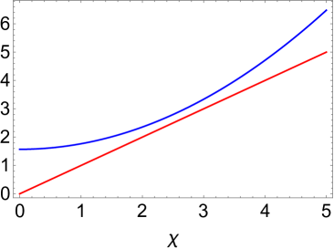
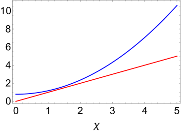
(a) (b) (c)

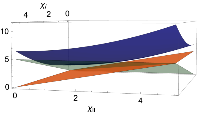
Figure 1: Integrated quantum metric (blue) bounded by the topological Euler number $\chi\geq 0$ (red). (a) Three-band $2+1$-Euler phases. (b) Four-band $2+2$-Euler phases with balanced Euler numbers $|\chi_{I}|=|\chi_{II}|=\chi$. (c) Four-band $2+2$-Euler phases with the imbalanced Euler numbers $|\chi_{I}|$ (green), $|\chi_{II}|$ (orange).

VIII.2.2 Four-band $2+2$-Euler phases

Considering again two-band subspaces, we find the same general bound on the metric

$$\text{tr}\,\boldsymbol{g}\geq 4|\boldsymbol{\omega}^{12}_{\theta\phi}|\,.$$ (178)

As a next step, using the four-band ansatz of Section V.4 for the balanced phases ($|\chi_{I}|=|\chi_{II}|=\chi$), we find

$$\left\{\begin{aligned} \text{tr}\,\boldsymbol{g}^{I}=\text{tr}\,\boldsymbol{g}^{II}&=\dfrac{1+\chi^{2}\sin^{2}\theta}{2}\,,\\ |\boldsymbol{\omega}^{I,12}_{\theta\phi}|=|\boldsymbol{\omega}^{II,12}_{\theta\phi}|&=\chi|\sin\theta|\,,\end{aligned}\right.$$ (179)

where $\{\boldsymbol{g}^{I}\,\boldsymbol{\omega}^{I,12}_{\theta\phi}\}$ ($\{\boldsymbol{g}^{II}\,\boldsymbol{\omega}^{II,12}_{\theta\phi}\}$) are the quantities obtained for the occupied (respectively, unoccupied) two-band subspace, which after integration gives

$$\left\{\begin{aligned} I^{I}_{1}&=I^{II}_{1}=\dfrac{\pi}{8}(2+\chi^{2})\,,\\ I^{I}_{2}&=I^{II}_{2}=\chi\,,\end{aligned}\right.$$ (180)

where here $\chi\in\mathbb{N}$. We again have a strict bound $I_{1}>I_{2}$.

If we however instead consider the imbalanced Euler phases ($|\chi_{I}|\neq|\chi_{II}|$), we find

$$\left\{\begin{aligned} \text{tr}\,\boldsymbol{g}^{I}&=\text{tr}\,\boldsymbol{g}^{II}=1+\dfrac{1}{4}(\chi_{I}^{2}+\chi_{II}^{2})\sin^{2}\theta\,,\\ |\boldsymbol{\omega}^{I,12}_{\theta\phi}|&=|\chi_{I}||\sin\theta|\,,~{}|\boldsymbol{\omega}^{II,12}_{\theta\phi}|=|\chi_{II}||\sin\theta|\,,\end{aligned}\right.$$ (181)

which, after integration, gives

$$\left\{\begin{aligned} I^{I}_{1}&=I^{II}_{1}=\dfrac{\pi}{16}(8+\chi_{I}^{2}+\chi_{II}^{2})\,,\\ I^{I}_{2}&=|\chi_{I}|\,,~{}I^{II}_{2}=|\chi_{II}|\,.\end{aligned}\right.$$ (182)

VIII.2.3 General numerical settings

The above analytical study can now be brought to the context of tight-binding settings, where the geometric structures must be computed numerically. In that respect, the fact that the sectional curvature of the submanifold $\mathcal{M}$, which is defined numerically from the evaluations of the Plücker vector, can be computed most efficiently from the Euler form of the numerically obtained tangent bundle $T\mathcal{M}$, represents a great advantage. In upcoming future work, we will show that the numerically integrated metric is its self bounded from below by the analytical expressions obtained above. This can be interpreted as the consequence that the metric of tight-binding models is degenerate since the mapping of the Brillouin zone to $\mathcal{M}$ fails to be an immersion, see the discussion in Section VI.3. This will be reported in detail elsewhere, but its general applicability shows the promise of the introduced perspective.

IX Conclusions and Discussion

We have shown that the Plücker embedding entails a versatile route to analyze geometric tensors and Riemannian structures for arbitrary $n$-band systems. Departing from simple two-band Chern models, we demonstrate how this embedding universally generalizes the quantum metric tensor in terms of a simple geometric viewpoint that formulates all relevant information. This concrete, non-redundant, approach however becomes even more far-reaching in evaluating general topological many-state systems hosting recently discovered multi-gap phases that arise by rather generic reality conditions. As such, our universal approach that manifests all relevant geometrical identities by appealing to a simple vector description, presents a powerful universal benchmark to evaluate physical topological systems.

The generic framework also provides a direct route towards a systematic modelling, highlighting the interplay of topology, geometry and direct descriptions in various situations. We outline how this approach accordingly can by utilized in numerous physical contexts. Indeed, as preliminary applications, we highlighted its manifestation in general perturbation theory that in turn can be used to analyze optical responses of many-band systems and outlined its use in defining quantum volumes that are of active interest to derive bounds on superfluidity or formulate ideal conditions to host fractional Chern states.

The above directions promise eminent potential to use the presented framework and explore several novel directions. These not only include analyzing novel interplays between topology and optical responses in many-band systems or utilizing the generalized metric and its bounds in different settings, but even reach to quantum computation and information. We already mentioned the relation to Cramér-Rao information bounds and reemphasize that the active scene of quantum metrology may directly profit from our framework. Moreover, we anticipate that the direct handle of many-band systems, also in terms of modelling, could induce new holonomic approaches to quantum compuation Pachos et al. (1999). In such approaches one essentially encodes information in a degenerate eigenspace of a parametric family of Hamiltonians, which basically thrives on defining generalized non-Abelian Berry connections that can be readily computed within our approach. We therefore believe that our results can set a benchmark for a wide range of novel fundamental insights as well as concrete physically relevant pursuits.

Appendix A Derivation of Equation (III)

We here detail the derivation of Eq. (III). To define a notion of distance $D$ between two states $V_{1}$ and $V_{2}$ in the Plücker embedding is we consider the canonical expression

$$D^{2}_{\text{Pl}}=1-\mathinner{\langle{V_{2}}|{V_{1}}\rangle}\mathinner{\langle{V_{1}}|{V_{2}}\rangle}$$ (183)

Assuming that $V_{2}$ differs from $V_{1}$ by an infinitesimal change $d\vec{x}$ in the parameters of the Hamiltonian, we then obtain

$$D^{2}_{\text{Pl}}=1-\mathinner{\langle{V(\vec{x}+\mathrm{d}\vec{x})}|{V(\vec{x})}\rangle}\mathinner{\langle{V(\vec{x})}|{V(\vec{x}+\mathrm{d}\vec{x})}\rangle}$$ (184)

Expressing this result in term of the eigenstates, the above implies

$$D^{2}_{\text{Pl}}=1-\mathinner{\langle{u_{1}(\vec{x}+\mathrm{d}\vec{x})\wedge\ldots\wedge u_{k}(\vec{x}+\mathrm{d}\vec{x})}|{u_{1}(\vec{x})\wedge\ldots\wedge u_{k}(\vec{x})}\rangle}$$

$$\mathinner{\langle{u_{1}(\vec{x})\wedge\ldots\wedge u_{k}(\vec{x})}|{u_{1}(\vec{x}+\mathrm{d}\vec{x})\wedge\ldots\wedge u_{k}(\vec{x}+\mathrm{d}\vec{x})}\rangle}$$

Expanding to second order in $\mathrm{d}\vec{x}$ then results in

$$D^{2}_{\text{Pl}}=1-\left\langle\left(\textstyle\sum_{i,j}u_{1}+\partial_{i}u_{1}\mathrm{d}x_{i}+\tfrac{1}{2}\partial_{i}\partial_{j}u_{1}\mathrm{d}x_{i}\mathrm{d}x_{j}\right)\wedge\ldots\wedge\left(\textstyle\sum_{i,j}u_{k}+\partial_{i}u_{k}\mathrm{d}x_{i}+\tfrac{1}{2}\partial_{i}\partial_{j}u_{k}\mathrm{d}x_{i}\mathrm{d}x_{j}\right)\right|$$

$$\left|u_{1}(\vec{x})\wedge\ldots\wedge u_{k}(\vec{x})\right\rangle\left\langle u_{1}(\vec{x})\wedge\ldots\wedge u_{k}(\vec{x})\right|$$

$$\left|\left(\textstyle\sum_{i,j}u_{1}+\partial_{i}u_{1}\mathrm{d}x_{i}+\tfrac{1}{2}\partial_{i}\partial_{j}u_{1}\mathrm{d}x_{i}\mathrm{d}x_{j}\right)\wedge\ldots\wedge\left(\textstyle\sum_{i,j}u_{k}+\partial_{i}u_{k}\mathrm{d}x_{i}+\tfrac{1}{2}\partial_{i}\partial_{j}u_{k}\mathrm{d}x_{i}\mathrm{d}x_{j}\right)\right\rangle,$$

where $i$ and $j$ indices denote components of the parameters $\vec{x}$. Multiplying out each inner product and keeping only terms to second order, we will have a few different categories of terms:

• The zeroth order term $\mathinner{\langle{u_{1}\wedge\ldots\wedge u_{k}}|{u_{1}\wedge\ldots\wedge u_{k}}\rangle}=1$

• First order terms containing a single $\partial_{i}u_{n}\mathrm{d}x_{i}$. A simple determinant calculation shows that these evaluate to $(\partial_{i}u_{n})^{\dagger}u_{n}\mathrm{d}x_{i}$

• Second order terms containing two instances of $\partial_{i}u_{n}\mathrm{d}x_{i}$. For these, we have not only $(\partial_{i}u_{n})^{\dagger}u_{n}(\partial_{j}u_{m})^{\dagger}u_{m}\mathrm{d}x_{i}\mathrm{d}x_{j}$ from the diagonal contribution to the determinant, but also an off-diagonal contribution $-(\partial_{i}u_{n})^{\dagger}u_{m}(\partial_{j}u_{m})^{\dagger}u_{n}\mathrm{d}x_{i}\mathrm{d}x_{j}$. To get the correct count, we require $n>m$ for these.

• Second order terms containing one instance of $\frac{1}{2}\partial_{i}\partial_{j}u_{n}\mathrm{d}x_{i}\mathrm{d}x_{j}$. This again has only a diagonal contribution to the determinant and thus evaluates to $\frac{1}{2}(\partial_{i}\partial_{j}u_{n})^{\dagger}u_{n}\mathrm{d}x_{i}\mathrm{d}x_{j}$

Applying the above, we arrive at

$$D^{2}_{\text{Pl}}=1-\left|1+\textstyle\sum_{i,j,n>m}(\partial_{i}u_{n})^{\dagger}u_{n}\mathrm{d}x_{i}+(\partial_{i}u_{n})^{\dagger}u_{n}(\partial_{j}u_{m})^{\dagger}u_{m}\mathrm{d}x_{i}\mathrm{d}x_{j}-(\partial_{i}u_{n})^{\dagger}u_{m}(\partial_{j}u_{m})^{\dagger}u_{n}\mathrm{d}x_{i}\mathrm{d}x_{j}\right.$$

$$\left.+\tfrac{1}{2}(\partial_{i}\partial_{j}u_{n})^{\dagger}u_{n}\mathrm{d}x_{i}\mathrm{d}x_{j}\right|^{2}.$$

Multiplying out the square and keeping only terms to second order, we then get

$$D^{2}_{\text{Pl}}=1-\left(1+\textstyle\sum_{i,j,n,m}2\mathrm{Re}\,\left((\partial_{i}u_{n})^{\dagger}u_{n}\right)\mathrm{d}x_{i}+(\partial_{i}u_{n})^{\dagger}u_{n}u_{m}^{\dagger}(\partial_{j}u_{m})\mathrm{d}x_{i}\mathrm{d}x_{j}\right.$$

$$+2\mathrm{Re}\,\left((\partial_{i}u_{n})^{\dagger}u_{n}(\partial_{j}u_{m})^{\dagger}u_{m}\right)_{n>m}\mathrm{d}x_{i}\mathrm{d}x_{j}-2\mathrm{Re}\,\left((\partial_{i}u_{n})^{\dagger}u_{m}(\partial_{j}u_{m})^{\dagger}u_{n}\right)_{n>m}\mathrm{d}x_{i}\mathrm{d}x_{j}$$

$$+\left.\tfrac{1}{2}\cdot 2\mathrm{Re}\,\left((\partial_{i}\partial_{j}u_{n})^{\dagger}u_{n}\right)\mathrm{d}x_{i}\mathrm{d}x_{j}\right)$$

The first order terms vanish because $(\partial_{i}u_{n})^{\dagger}u_{n}$ is pure imaginary. We can drop the $\mathrm{Re}\,$ on most of the second order terms because they are products of two such imaginary terms. For the $n>m$ terms, we extend to a sum over all $n,m$ by absorbing a factor of $2$ and noticing that the $n=m$ terms internally cancel.

$$D^{2}_{\text{Pl}}=-\textstyle\sum_{i,j,n,m}\left((\partial_{i}u_{n})^{\dagger}u_{n}u_{m}^{\dagger}(\partial_{j}u_{m})+(\partial_{i}u_{n})^{\dagger}u_{n}(\partial_{j}u_{m})^{\dagger}u_{m}-(\partial_{i}u_{n})^{\dagger}u_{m}(\partial_{j}u_{m})^{\dagger}u_{n}\right.$$

$$+\left.\mathrm{Re}\,\left((\partial_{i}\partial_{j}u_{n})^{\dagger}u_{n}\right)\right)\mathrm{d}x_{i}\mathrm{d}x_{j}$$

We also have that $(\partial_{i}u_{n})^{\dagger}u_{n}u_{m}^{\dagger}(\partial_{j}u_{m})=-(\partial_{i}u_{n})^{\dagger}u_{n}(\partial_{j}u_{m})^{\dagger}u_{m}$, so the first two terms cancel. We are left with

$$D^{2}_{\text{Pl}}=-\textstyle\sum_{i,j,n,m}\left(-(\partial_{i}u_{n})^{\dagger}u_{m}(\partial_{j}u_{m})^{\dagger}u_{n}+\mathrm{Re}\,\left((\partial_{i}\partial_{j}u_{n})^{\dagger}u_{n}\right)\right)\mathrm{d}x_{i}\mathrm{d}x_{j}$$

Integrating by parts, this can be written

$$D^{2}_{\text{Pl}}=-\textstyle\sum_{i,j,n,m}\left((\partial_{i}u_{n})^{\dagger}u_{m}u_{m}^{\dagger}\partial_{j}u_{n}+\mathrm{Re}\,\left(\partial_{j}((\partial_{i}u_{n})^{\dagger}u_{n})-(\partial_{i}u_{n})^{\dagger}\partial_{j}u_{n}\right)\right)\mathrm{d}x_{i}\mathrm{d}x_{j}$$

The first term is pure real and the first term inside the $\mathrm{Re}\,$ is pure imaginary, so this reduces to

$$D^{2}_{\text{Pl}}=\textstyle\sum_{i,j,n,m}\mathrm{Re}\,\left((\partial_{i}u_{n})^{\dagger}\partial_{j}u_{n}-(\partial_{i}u_{n})^{\dagger}u_{m}u_{m}^{\dagger}\partial_{j}u_{n}\right)\mathrm{d}x_{i}\mathrm{d}x_{j}$$

Switching to Dirac notation, we discern the usual quantum metric

$$g_{ij}=\sum_{n,m\in\text{occ}}\mathrm{Re}\,\mathinner{\langle{\partial_{i}u_{n}}|}\left(\mathbb{I}-\mathinner{|{u_{m}}\rangle}\mathinner{\langle{u_{m}}|}\right)\mathinner{|{\partial_{j}u_{n}}\rangle},\quad D^{2}_{\text{Pl}}=\sum_{i,j}g_{ij}\mathrm{d}x_{i}\mathrm{d}x_{j}$$

We thus observe that the usual notion of infinitesimal distance between two manifolds of states $D^{2}$ corresponds exactly to the distance we defined in the Plücker embedding,

$$D^{2} = D^{2}_{\text{Pl}}$$

$$= 1-\mathinner{\langle{V(x+\mathrm{d}x)}|{V(x)}\rangle}\mathinner{\langle{V(x)}|{V(x+\mathrm{d}x)}\rangle}.$$

To write the quantum metric in the Plücker embedding, we would then go through the exercise of expanding $V(x+dx)$ and rearranging $D^{2}_{\text{Pl}}$ into the form $g_{ij}\mathrm{d}x_{i}\mathrm{d}x_{j}$. This however amounts to the same derivation one would do for the single band case in the standard formalism. Therefore we irectly infer that the usual quantum metric expressed in the Plücker embedding is

$$g_{ij}=\mathrm{Re}\,\left(\mathinner{\langle{\partial_{i}V}|{\partial_{j}V}\rangle}-\mathinner{\langle{\partial_{i}V}|{V}\rangle}\mathinner{\langle{V}|{\partial_{j}V}\rangle}\right).$$ (185)

Appendix B Alternative parametrization of $\widetilde{\mathsf{Gr}}_{2,4}^{\mathbb{R}}$

We start with the parametrization of a generic element of $\mathsf{SO}(4)$ as de Guise et al. (2018)

$$R^{4B}(\theta_{1}\cdots\theta_{6})=e^{\theta_{1}L_{12}}e^{\theta_{2}L_{13}}e^{\theta_{3}L_{14}}e^{\theta_{4}L_{23}}e^{\theta_{5}L_{24}}e^{\theta_{6}L_{34}}\,,$$ (186)

with the angular momentum matrices $[L_{ij}]_{\alpha\beta}=-\delta_{\alpha i}\delta_{\beta j}+\delta_{\alpha j}\delta_{\beta i}$ for all pairs $(i,j)\in I_{2}=\{(a,b)|1\leq a<b\leq 4\}=\{(1,2),(1,3),(1,4),(2,3),(2,4),(3,4)\}$, that form a basis of $\mathsf{so}(4)$ (dim $\mathsf{so}(4)$=6). A direct inspection shows that $\theta_{6}$ is a pure gauge sign and we thus set $\theta_{6}=0$. In the end, we need a reduction to a maximum of $4$ principal angles that parametrize the four-dimensional Grassmannian $\widetilde{\mathsf{Gr}}_{2,4}^{\mathbb{R}}$. For this we take the wedge products

$$V_{I}=u_{1}\wedge u_{2}\,,\;V_{II}=u_{3}\wedge u_{4}\,,$$ (187)

that both define six-dimensional vectors in $\bigwedge^{2}\left(\mathbb{R}^{4}\right)$ and written in the basis $\{\check{\boldsymbol{e}}_{ij}=e_{i}\wedge e_{j}\}_{(i,j)\in I_{2}}$ (again with $\{e_{i}\}_{i=1}^{4}$ the Cartersian basis of $\mathbb{R}^{4}$). We now take the linear combinations

$$V_{\pm}=V_{I}\pm V_{II}\,,$$ (188)

and write these as

$$V_{\pm}=\check{\boldsymbol{e}}_{ij}\,[V_{\pm}]_{ij}=\check{\boldsymbol{e}}_{ij}^{\prime}\,[V_{\pm}^{\prime}]_{ij}\,,$$ (189)

in the new basis,

$$\left[\begin{array}[]{c}\check{\boldsymbol{e}}_{12}^{\prime}\\ \check{\boldsymbol{e}}_{13}^{\prime}\\ \check{\boldsymbol{e}}_{14}^{\prime}\\ \check{\boldsymbol{e}}_{23}^{\prime}\\ \check{\boldsymbol{e}}_{24}^{\prime}\\ \check{\boldsymbol{e}}_{34}^{\prime}\end{array}\right]^{\top}=\left[\begin{array}[]{c}\check{\boldsymbol{e}}_{12}\\ \check{\boldsymbol{e}}_{13}\\ \check{\boldsymbol{e}}_{14}\\ \check{\boldsymbol{e}}_{23}\\ \check{\boldsymbol{e}}_{24}\\ \check{\boldsymbol{e}}_{34}\end{array}\right]^{\top}\cdot\dfrac{1}{2}\left[\begin{array}[]{rrrrrr}0&1&0&0&-1&0\\ 0&0&1&1&0&0\\ 1&0&0&0&0&1\\ 0&1&0&0&1&0\\ 0&0&1&-1&0&0\\ 1&0&0&0&0&-1\end{array}\right]\,.$$ (190)

Then, by setting

$$(\theta_{1},\theta_{2}) =(0,0)\,,$$ (191)

$$(\theta_{3},\theta_{4}) =\dfrac{1}{2}(\phi_{+}+\phi_{-},\phi_{+}-\phi_{-})\,,$$

$$\theta_{5} =-\theta+\pi/2\,,$$

we finally obtain

$$V_{+}^{\prime} =(\sin\phi_{+}\sin\theta,\cos\theta,\cos\phi_{+}\sin\theta,0,0,0)\,,$$ (192)

$$V_{-}^{\prime} =(0,0,0,-\sin\phi_{-}\sin\theta,\cos\theta,\cos\phi_{-}\sin\theta)\,,$$

such that each Plücker vector ($V_{\pm}^{\prime}$) defines a two-sphere ($\mathbb{S}^{2}_{\pm}$) within one three-dimensional half of the six-dimensional vector space $\bigwedge^{2}(\mathbb{R}^{4})=V_{+}\oplus V_{-}\cong\mathbb{R}^{3}\oplus\mathbb{R}^{3}$, i.e. $V_{\pm}^{\prime}\in\mathbb{S}^{2}_{\pm}\in V_{\pm}$. We remark that by only keeping three angles, $V_{\pm}^{\prime}$ do not cover the whole of $\mathsf{Gr}_{2,4}^{\mathbb{R}}$. Nevertheless, we do capture the two sub-dimensional spheres contained in the four-dimensional Grassmannian and this is sufficient to fully characterize the 2D Euler topology, as we now show.

Defining the unit vectors

$$\boldsymbol{n}_{+} =(\cos\phi_{+}\sin\theta,\sin\phi_{+}\sin\theta,\cos\theta)\in\mathbb{S}^{2}_{+}\,,$$ (193a)

$$\boldsymbol{n}_{-} =(\cos\phi_{+}\sin\theta,\sin\phi_{+}\sin\theta,\cos\theta)\in\mathbb{S}^{2}_{-}\,,$$

and substituting the parameters Eq. (191) in the $$2+2 E_{1}=E_{2}=-E_{3}=-E_{4}=-1$$-Hamiltonian form Eq. (39), we get, after setting ,

$$H^{\mathbb{R},2+2}[\boldsymbol{n}_{+},\boldsymbol{n}_{-}]= \,n^{3}_{-}\left(-n^{3}_{+}\Gamma_{33}+n^{2}_{+}\Gamma_{31}-n^{1}_{+}\Gamma_{10}\right)$$ (193b)

$$+ \,n^{1}_{-}\left(+n^{3}_{+}\Gamma_{13}-n^{2}_{+}\Gamma_{11}-n^{1}_{+}\Gamma_{30}\right)$$

$$+ \,n^{2}_{-}\left(+n^{3}_{+}\Gamma_{01}+n^{2}_{+}\Gamma_{03}+n^{1}_{+}\Gamma_{22}\right)\,,$$

$$= \,\boldsymbol{n}_{+}^{\top}\cdot\underline{\Gamma}\cdot\boldsymbol{n}_{-}\,,$$

with the tensor

$$\underline{\Gamma}=\left(\begin{array}[]{rrr}-\Gamma_{30}&\Gamma_{22}&-\Gamma_{10}\\ -\Gamma_{11}&\Gamma_{03}&\Gamma_{31}\\ \Gamma_{13}&\Gamma_{01}&-\Gamma_{33}\end{array}\right)\,.$$ (193c)

We note that the above derivation differs from the previous ones exposed in Bouhon et al. (2020b); Bouhon and Slager (2022) by the initial choice of the parametrization of the $\mathsf{SO}(4)$ matrix representing the frame of eigenvectors.

If we set

$$(\phi_{+},\phi_{-}) =(q_{+},q_{-})\,\phi_{0}\,,\;\theta=\theta_{0}\,,$$ (194)

$$q_{+},q_{-} \in\mathbb{Z}\,,$$

such that $\boldsymbol{n}_{+}$ ($\boldsymbol{n}_{-}$) wraps the sphere $\mathbb{S}^{2}_{+}$ ($\mathbb{S}^{2}_{-}$) a number of times $q_{+}$ ($q_{-}$) whenever $(\phi_{0},\theta_{0})$ covers one time the base sphere $\mathbb{S}^{2}_{0}$. The direct computation of the Euler two-form for the occupied and unoccupied two-band subspaces then gives

$$\mathtt{F}_{\mathbb{S}^{2}_{0}}[\{u_{1},u_{2}\}] =-\dfrac{q_{+}+q_{-}}{2}\sin\theta_{0}\,,$$ (195)

$$\mathtt{F}_{\mathbb{S}^{2}_{0}}[\{u_{3},u_{4}\}] =-\dfrac{q_{+}-q_{-}}{2}\sin\theta_{0}\,,$$

and accordingly Euler classes

$$\chi_{I,\mathbb{S}^{2}_{0}} =-(q_{+}+q_{-})\in\mathbb{Z}\,,$$ (196)

$$\chi_{II,\mathbb{S}^{2}_{0}} =-(q_{+}-q_{-})\in\mathbb{Z}\,.$$

Appendix C Orientability of Euler homotopy classes

The fact that we have used the oriented Grassmannian for the Plücker embedding must now be corrected since the Bloch Hamiltonian are only orientable, and the phases are classified by the free homotopy set (i.e. no base point), together allowing the reversal of the orientation through an adiabatic transformation (automorphism of $\pi_{2}$ by the action of $\pi_{1}$) Bouhon et al. (2020b). The strict homotopy classification gives the following equivalence

$$(\chi_{I},\chi_{II})\simeq(-\chi_{I},-\chi_{II})\,.$$ (197)

Whenever the partial gap between two bands of the same subspace (that is closed by nodal points) closes completely (i.e. at every momentum), or in other words, when a band inversion takes place between these two bands such that they become fully degenerate, there is yet a further homotopy equivalence of signed Euler classes, namely

$$\chi_{I}\simeq-\chi_{I}\,,\;\chi_{II}\simeq-\chi_{II}\,,$$ (198)

see Bouhon and Slager (2022) for a detailed discussion.

There only remains to pullback the base sphere $\mathbb{S}^{2}_{0}$ to the torus Brillouin zone via the map Eq. (27) such that the resulting $2+2$-Bloch Hamiltonian has an Euler topology exhaustively captures by

$$(\chi_{I,\mathbb{T}^{2}},\chi_{II,\mathbb{T}^{2}})=(\chi_{I,\mathbb{S}^{2}_{0}},\chi_{II,\mathbb{S}^{2}_{0}})\in\mathbb{Z}^{2}/\sim\,,$$ (199)

with $\sim$ for the above homotopy equivalences.

References

- Qi and Zhang (2011) Xiao-Liang Qi and Shou-Cheng Zhang, “Topological insulators and superconductors,” Rev. Mod. Phys. 83, 1057–1110 (2011).
- Hasan and Kane (2010) M. Z. Hasan and C. L. Kane, “Colloquium,” Rev. Mod. Phys. 82, 3045–3067 (2010).
- Armitage et al. (2018) N. P. Armitage, E. J. Mele, and Ashvin Vishwanath, “Weyl and dirac semimetals in three-dimensional solids,” Rev. Mod. Phys. 90, 015001 (2018).
- Fu (2011) Liang Fu, “Topological crystalline insulators,” Phys. Rev. Lett. 106, 106802 (2011).
- Slager et al. (2012) Robert-Jan Slager, Andrej Mesaros, Vladimir Juričić, and Jan Zaanen, “The space group classification of topological band-insulators,” Nat. Phys. 9, 98 (2012).
- Kruthoff et al. (2017) Jorrit Kruthoff, Jan de Boer, Jasper van Wezel, Charles L. Kane, and Robert-Jan Slager, “Topological classification of crystalline insulators through band structure combinatorics,” Phys. Rev. X 7, 041069 (2017).
- Po et al. (2017) Hoi Chun Po, Ashvin Vishwanath, and Haruki Watanabe, “Symmetry-based indicators of band topology in the 230 space groups,” Nat. Commun. 8, 50 (2017).
- Bradlyn et al. (2017) Barry Bradlyn, L. Elcoro, Jennifer Cano, M. G. Vergniory, Zhijun Wang, C. Felser, M. I. Aroyo, and B. Andrei Bernevig, “Topological quantum chemistry,” Nature 547, 298 (2017).
- Slager (2019) Robert-Jan Slager, “The translational side of topological band insulators,” Journal of Physics and Chemistry of Solids 128, 24 (2019).
- Scheurer and Slager (2020) Mathias S. Scheurer and Robert-Jan Slager, “Unsupervised machine learning and band topology,” Phys. Rev. Lett. 124, 226401 (2020).
- Schrunk et al. (2022) Benjamin Schrunk, Yevhen Kushnirenko, Brinda Kuthanazhi, Junyeong Ahn, Lin-Lin Wang, Evan O’Leary, Kyungchan Lee, Andrew Eaton, Alexander Fedorov, Rui Lou, Vladimir Voroshnin, Oliver J. Clark, Jaime Sánchez-Barriga, Sergey L. Bud’ko, Robert-Jan Slager, Paul C. Canfield, and Adam Kaminski, “Emergence of fermi arcs due to magnetic splitting in an antiferromagnet,” Nature 603, 610–615 (2022).
- Rhim et al. (2018) Jun-Won Rhim, Jens H. Bardarson, and Robert-Jan Slager, “Unified bulk-boundary correspondence for band insulators,” Phys. Rev. B 97, 115143 (2018).
- Kitaev (2009) Alexei Kitaev, “Periodic table for topological insulators and superconductors,” AIP Conference Proceedings 1134, 22–30 (2009).
- Schnyder et al. (2008) Andreas P. Schnyder, Shinsei Ryu, Akira Furusaki, and Andreas W. W. Ludwig, “Classification of topological insulators and superconductors in three spatial dimensions,” Phys. Rev. B 78, 195125 (2008).
- Song et al. (2018) Zhida Song, Tiantian Zhang, Zhong Fang, and Chen Fang, “Quantitative mappings between symmetry and topology in solids,” Nature communications 9, 1–7 (2018).
- Bouhon et al. (2021) Adrien Bouhon, Gunnar F. Lange, and Robert-Jan Slager, “Topological correspondence between magnetic space group representations and subdimensions,” Phys. Rev. B 103, 245127 (2021).
- Elcoro et al. (2021) Luis Elcoro, Benjamin J. Wieder, Zhida Song, Yuanfeng Xu, Barry Bradlyn, and B. Andrei Bernevig, “Magnetic topological quantum chemistry,” Nature Communications 12, 1–10 (2021).
- Watanabe et al. (2018) Haruki Watanabe, Hoi Chun Po, and Ashvin Vishwanath, “Structure and topology of band structures in the 1651 magnetic space groups,” Science Advances 4 (2018).
- Kemp et al. (2022) Cameron J. D. Kemp, Nigel R. Cooper, and F. Nur Ünal, “Nested-sphere description of the -level chern number and the generalized bloch hypersphere,” Phys. Rev. Res. 4, 023120 (2022).
- Volovik and Mineev (2018) GE Volovik and VP Mineev, “Investigation of singularities in superfluid he3 in liquid crystals by the homotopic topology methods,” in Basic Notions Of Condensed Matter Physics (CRC Press, 2018) pp. 392–401.
- Van Mechelen et al. (2022) Todd Van Mechelen, Sathwik Bharadwaj, Zubin Jacob, and Robert-Jan Slager, “Optical -insulators: Topological obstructions to optical wannier functions in the atomistic susceptibility tensor,” Phys. Rev. Res. 4, 023011 (2022).
- Chiu et al. (2016) Ching-Kai Chiu, Jeffrey C. Y. Teo, Andreas P. Schnyder, and Shinsei Ryu, “Classification of topological quantum matter with symmetries,” Rev. Mod. Phys. 88, 035005 (2016).
- Provost and Vallee (1980) JP Provost and G Vallee, “Riemannian structure on manifolds of quantum states,” Communications in Mathematical Physics 76, 289–301 (1980).
- Resta (2011) R. Resta, “The insulating state of matter: a geometrical theory,” The European Physical Journal B 79, 121–137 (2011).
- Ozawa and Goldman (2018) Tomoki Ozawa and Nathan Goldman, “Extracting the quantum metric tensor through periodic driving,” Phys. Rev. B 97, 201117 (2018).
- Tran et al. (2017) Duc Thanh Tran, Alexandre Dauphin, Adolfo G. Grushin, Peter Zoller, and Nathan Goldman, “Probing topology by “heating”: Quantized circular dichroism in ultracold atoms,” Science Advances 3 (2017), 10.1126/sciadv.1701207.
- Salerno et al. (2020) Grazia Salerno, Nathan Goldman, and Giandomenico Palumbo, “Floquet-engineering of nodal rings and nodal spheres and their characterization using the quantum metric,” Phys. Rev. Res. 2, 013224 (2020).
- de Juan et al. (2017) Fernando de Juan, Adolfo G. Grushin, Takahiro Morimoto, and Joel E Moore, “Quantized circular photogalvanic effect in weyl semimetals,” Nature Communications 8, 15995 (2017).
- Mera and Ozawa (2021) Bruno Mera and Tomoki Ozawa, “Kähler geometry and chern insulators: Relations between topology and the quantum metric,” Phys. Rev. B 104, 045104 (2021).
- Palumbo (2021) Giandomenico Palumbo, “Non-abelian tensor berry connections in multiband topological systems,” Phys. Rev. Lett. 126, 246801 (2021).
- Yu et al. (2022) Min Yu, Xiangbei Li, Yaoming Chu, Bruno Mera, F. Nur Ünal, Pengcheng Yang, Yu Liu, Nathan Goldman, and Jianming Cai, “Experimental demonstration of topological bounds in quantum metrology,” arXiv:2206.00546 (2022), 10.48550/arxiv.2206.00546.
- Li et al. (2022) Changhao Li, Mo Chen, and Paola Cappellaro, “A geometric perspective: experimental evaluation of the quantum cramer-rao bound,” arXiv:2204.13777 (2022), 10.48550/arxiv.2204.13777.
- Peotta and Törmä (2015) Sebastiano Peotta and Päivi Törmä, “Superfluidity in topologically nontrivial flat bands,” Nature communications 6, 1–9 (2015).
- Törmä et al. (2021) Päivi Törmä, Sebastiano Peotta, and Bogdan A Bernevig, “Superfluidity and quantum geometry in twisted multilayer systems,” arXiv preprint arXiv:2111.00807 (2021).
- Begholtz and Liu (2013) Emil J. Begholtz and Zhao Liu, “Topological flat band models and fractional chern insulators,” International Journal of Modern Physics B 27, 1330017 (2013).
- Rhim et al. (2020) Jun-Won Rhim, Kyoo Kim, and Bohm-Jung Yang, “Quantum distance and anomalous landau levels of flat bands,” Nature 584, 59–63 (2020).
- Herzog-Arbeitman et al. (2022) Jonah Herzog-Arbeitman, Valerio Peri, Frank Schindler, Sebastian D. Huber, and B. Andrei Bernevig, “Superfluid weight bounds from symmetry and quantum geometry in flat bands,” Phys. Rev. Lett. 128, 087002 (2022).
- Parker et al. (2021) Daniel Parker, Patrick Ledwith, Eslam Khalaf, Tomohiro Soejima, Johannes Hauschild, Yonglong Xie, Andrew Pierce, Michael P Zaletel, Amir Yacoby, and Ashvin Vishwanath, “Field-tuned and zero-field fractional chern insulators in magic angle graphene,” arXiv preprint arXiv:2112.13837 (2021).
- Julku et al. (2016) Aleksi Julku, Sebastiano Peotta, Tuomas I. Vanhala, Dong-Hee Kim, and Päivi Törmä, “Geometric origin of superfluidity in the lieb-lattice flat band,” Phys. Rev. Lett. 117, 045303 (2016).
- Peri et al. (2021) Valerio Peri, Zhi-Da Song, B. Andrei Bernevig, and Sebastian D. Huber, “Fragile topology and flat-band superconductivity in the strong-coupling regime,” Phys. Rev. Lett. 126, 027002 (2021).
- Bouhon et al. (2020a) Adrien Bouhon, QuanSheng Wu, Robert-Jan Slager, Hongming Weng, Oleg V. Yazyev, and Tomáš Bzdušek, “Non-abelian reciprocal braiding of weyl points and its manifestation in zrte,” Nature Physics 16, 1137–1143 (2020a).
- Ahn et al. (2019a) Junyeong Ahn, Sungjoon Park, and Bohm-Jung Yang, “Failure of nielsen-ninomiya theorem and fragile topology in two-dimensional systems with space-time inversion symmetry: Application to twisted bilayer graphene at magic angle,” Phys. Rev. X 9, 021013 (2019a).
- Bouhon et al. (2020b) Adrien Bouhon, Tomáš Bzdušek, and Robert-Jan Slager, “Geometric approach to fragile topology beyond symmetry indicators,” Phys. Rev. B 102, 115135 (2020b).
- Jiang et al. (2021a) Tianshu Jiang, Qinghua Guo, Ruo-Yang Zhang, Zhao-Qing Zhang, Biao Yang, and C. T. Chan, “Four-band non-abelian topological insulator and its experimental realization,” Nature Communications 12, 6471 (2021a).
- Guo et al. (2021) Qinghua Guo, Tianshu Jiang, Ruo-Yang Zhang, Lei Zhang, Zhao-Qing Zhang, Biao Yang, Shuang Zhang, and C. T. Chan, “Experimental observation of non-abelian topological charges and edge states,” Nature 594, 195–200 (2021).
- Jiang et al. (2022) Bin Jiang, Adrien Bouhon, Shi-Qiao Wu, Ze-Lin Kong, Zhi-Kang Lin, Robert-Jan Slager, and Jian-Hua Jiang, “Experimental observation of meronic topological acoustic euler insulators,” arXiv preprint arXiv:2205.03429 (2022).
- Jiang et al. (2021b) Bin Jiang, Adrien Bouhon, Zhi-Kang Lin, Xiaoxi Zhou, Bo Hou, Feng Li, Robert-Jan Slager, and Jian-Hua Jiang, “Experimental observation of non-abelian topological acoustic semimetals and their phase transitions,” Nature Physics 17, 1239–1246 (2021b).
- Zhao et al. (2022) W. D. Zhao, Y. B. Yang, Y. Jiang, Z. C. Mao, W. X. Guo, L. Y. Qiu, G. X. Wang, L. Yao, L. He, Z. C. Zhou, Y. Xu, and L. M. Duan, “Observation of topological euler insulators with a trapped-ion quantum simulator,” (2022), arXiv:2201.09234 [quant-ph] .
- Park et al. (2021) Sungjoon Park, Yoonseok Hwang, Hong Chul Choi, and Bohm Jung Yang, “Topological acoustic triple point,” Nature Communications 12, 1–9 (2021).
- Ünal et al. (2020) F. Nur Ünal, Adrien Bouhon, and Robert-Jan Slager, “Topological euler class as a dynamical observable in optical lattices,” Phys. Rev. Lett. 125, 053601 (2020).
- Peng et al. (2022a) Bo Peng, Adrien Bouhon, Robert-Jan Slager, and Bartomeu Monserrat, “Multigap topology and non-abelian braiding of phonons from first principles,” Phys. Rev. B 105, 085115 (2022a).
- Könye et al. (2021) Viktor Könye, Adrien Bouhon, Ion Cosma Fulga, Robert-Jan Slager, Jeroen van den Brink, and Jorge I. Facio, “Chirality flip of weyl nodes and its manifestation in strained ,” Phys. Rev. Research 3, L042017 (2021).
- Bouhon et al. (2023a) Adrien Bouhon, Yan-Qing Zhu, Robert-Jan Slager, and Giandomenico Palumbo, “Second euler number in four dimensional synthetic matter,” arXiv:2301.08827 (2023a), 10.48550/arxiv.2301.08827.
- Peng et al. (2022b) Bo Peng, Adrien Bouhon, Bartomeu Monserrat, and Robert-Jan Slager, “Phonons as a platform for non-abelian braiding and its manifestation in layered silicates,” Nature Communications 13, 423 (2022b).
- Lange et al. (2021) Gunnar F. Lange, Adrien Bouhon, and Robert-Jan Slager, “Subdimensional topologies, indicators, and higher order boundary effects,” Phys. Rev. B 103, 195145 (2021).
- Lange et al. (2022) Gunnar F. Lange, Adrien Bouhon, Bartomeu Monserrat, and Robert-Jan Slager, “Topological continuum charges of acoustic phonons in two dimensions and the nambu-goldstone theorem,” Phys. Rev. B 105, 064301 (2022).
- Slager et al. (2022) Robert-Jan Slager, Adrien Bouhon, and F. Nur Ünal, “Floquet multi-gap topology: Non-abelian braiding and anomalous dirac string phase,” arXiv:2208.12824 (2022), 10.48550/ARXIV.2208.12824.
- Ahn et al. (2021) Junyeong Ahn, Guang-Yu Guo, Naoto Nagaosa, and Ashvin Vishwanath, “Riemannian geometry of resonant optical responses,” Nature Physics 18, 290–295 (2021).
- Ma et al. (2010) Yu-Quan Ma, Shu Chen, Heng Fan, and Wu-Ming Liu, “Abelian and non-abelian quantum geometric tensor,” Phys. Rev. B 81, 245129 (2010).
- Note (1) More precisely, the classifying space is the homogeneous space that captures the gauge structure of the spectral decomposition of the Bloch Hamiltonian, with the Lie group of diagonalizing matrices and the group of gauge transformations that preserve the spectral decomposition between disconnected bands. Then, the homotopy classes of Bloch Hamiltonian of -dimensional systems, , can be decomposed into the homotopy groups .
- Bouhon and Slager (2022) Adrien Bouhon and Robert-Jan Slager, “Multi-gap topological conversion of euler class via band-node braiding: minimal models, -linked nodal rings, and chiral heirs,” arXiv:2203.16741 (2022), 10.48550/ARXIV.2203.16741.
- Wu et al. (2019) QuanSheng Wu, Alexey A. Soluyanov, and Tomáš Bzdušek, “Non-abelian band topology in noninteracting metals,” Science 365, 1273–1277 (2019).
- Alexander et al. (2012) Gareth P. Alexander, Bryan Gin-ge Chen, Elisabetta A. Matsumoto, and Randall D. Kamien, “Colloquium: Disclination loops, point defects, and all that in nematic liquid crystals,” Rev. Mod. Phys. 84, 497–514 (2012).
- Liu et al. (2016) Ke Liu, Jaakko Nissinen, Robert-Jan Slager, Kai Wu, and Jan Zaanen, “Generalized liquid crystals: Giant fluctuations and the vestigial chiral order of , , and matter,” Phys. Rev. X 6, 041025 (2016).
- Beekman et al. (2017) Aron J. Beekman, Jaakko Nissinen, Kai Wu, Ke Liu, Robert-Jan Slager, Zohar Nussinov, Vladimir Cvetkovic, and Jan Zaanen, “Dual gauge field theory of quantum liquid crystals in two dimensions,” Physics Reports 683, 1 – 110 (2017).
- de Guise et al. (2018) Hubert de Guise, Olivia Di Matteo, and Luis L. Sánchez-Soto, “Simple factorization of unitary transformations,” Phys. Rev. A 97, 022328 (2018).
- Ahn and Yang (2019) Junyeong Ahn and Bohm-Jung Yang, “Symmetry representation approach to topological invariants in -symmetric systems,” Phys. Rev. B 99, 235125 (2019).
- Bouhon et al. (2023b) Adrien Bouhon, Tomáš Bzdušek, and Robert-Jan Slager, “Quantization of 1d non-abelian multi-gap topological charges and the absence thereof,” to appear (2023b).
- Chen et al. (2022) Siyu Chen, Adrien Bouhon, Robert-Jan Slager, and Bartomeu Monserrat, “Non-abelian braiding of weyl nodes via symmetry-constrained phase transitions,” Phys. Rev. B 105, L081117 (2022).
- Chebotarev and Teretenkov (2014) Alexander M. Chebotarev and Alexander E. Teretenkov, “Singular value decomposition for the takagi factorization of symmetric matrices,” Applied Mathematics and Computation 234, 380–384 (2014).
- Hatcher (2003) A. Hatcher, Vector Bundles and K-Theory (Unpublished, 2003).
- Panati (2007) Gianluca Panati, “Triviality of bloch and bloch-dirac bundles,” Ann. Henri Poincaré 8, 995?1011 (2007).
- Ahn et al. (2018) Junyeong Ahn, Dongwook Kim, Youngkuk Kim, and Bohm-Jung Yang, “Band topology and linking structure of nodal line semimetals with monopole charges,” Phys. Rev. Lett. 121, 106403 (2018).
- Xie et al. (2020a) Fang Xie, Zhida Song, Biao Lian, and B. Andrei Bernevig, “Topology-bounded superfluid weight in twisted bilayer graphene,” Phys. Rev. Lett. 124, 167002 (2020a).
-
Note (2)