plaintop
\restylefloattable
\floatsetup[figure]subcapbesideposition = top
11institutetext:
Computer Science and Engineering,
The Ohio State University, Columbus, OH 43210, USA
11email: {ning.104}@osu.edu 22institutetext: Machine Learning Department, NEC Labs, Princeton, NJ 08540, USA
22email: {renqiang}@nec-labs.com 33institutetext: Digital Technologies Research Centre, National Research Council Canada, Ontario, Canada 44institutetext: Department of Medicine, Baylor College of Medicine, Houston, TX 77030, USA 55institutetext: NEC Oncolmmunity AS, Oslo Cancer Cluster, Innovation Park, Ullernchausséen 64, 0379, Oslo, Norway 66institutetext: Biomedical Informatics, The Ohio State University, Columbus, OH 43210, USA 77institutetext: Translational Data Analytics Institute, The Ohio State University, Columbus, OH 43210, USA
T-Cell Receptor Optimization with Reinforcement Learning and Mutation Polices for Precision Immunotherapy
Abstract
T cells monitor the health status of cells by identifying foreign peptides displayed on their surface. T-cell receptors (TCRs), which are protein complexes found on the surface of T cells, are able to bind to these peptides. This process is known as TCR recognition and constitutes a key step for immune response. Optimizing TCR sequences for TCR recognition represents a fundamental step towards the development of personalized treatments to trigger immune responses killing cancerous or virus-infected cells. In this paper, we formulated the search for these optimized TCRs as a reinforcement learning () problem, and presented a framework with a mutation policy using proximal policy optimization. mutates TCRs into effective ones that can recognize given peptides. leverages a reward function that combines the likelihoods of mutated sequences being valid TCRs measured by a new scoring function based on deep autoencoders, with the probabilities of mutated sequences recognizing peptides from a peptide-TCR interaction predictor. We compared with multiple baseline methods and demonstrated that significantly outperforms all the baseline methods to generate positive binding and valid TCRs. These results demonstrate the potential of for both precision immunotherapy and peptide-recognizing TCR motif discovery.
Keywords:
T-cell Receptor Immunotherapy Reinforcement Learning Biological Sequence Design1 Introduction
Immunotherapy is a fundamental treatment for human diseases, which uses a person’s immune system to fight diseases [35, 10, 36]. In the immune system, immune response is triggered by cytotoxic T cells which are activated by the engagement of the T cell receptors (TCRs) with immunogenic peptides presented by Major Histocompatibility Complex (MHC) proteins on the surface of infected or cancerous cells. The recognition of these foreign peptides is determined by the interactions between the peptides and TCRs on the surface of T cells. This process is known as TCR recognition and constitutes a key step for immune response [9, 12]. Adoptive T cell immunotherapy (ACT), which has been a promising cancer treatment, genetically modifies the autologous T cells taken from patients in laboratory experiments, after which the modified T cells are infused into patients’ bodies to fight cancer. As one type of ACT therapies, TCR T cell (TCR-T) therapy directly modifies the TCRs of T cells to increase the binding affinities, which makes it possible to recognize and kill tumor cells effectively [27]. TCR is a heterodimeric protein with an chain and a chain. Each chain has three loops as complementary determining regions (CDR): CDR1, CDR2 and CDR3. CDR1 and CDR2 are primarily responsible for interactions with MHC, and CDR3 interacts with peptides [26]. The CDR3 of the chain has a higher degree of variations and is therefore arguably mainly responsible for the recognition of foreign peptides [20]. In this paper, we focused on the optimization of the CDR3 sequence of chain in TCRs to enhance their binding affinities against peptide antigens, and we conducted the optimization through novel reinforcement learning. The success of our approach will have the potential to guide TCR-T therapy design. For the sake of simplicity, when we refer to TCRs in the rest of the paper, we mean the CDR3 of chain in TCRs.
Despite the significant promise of TCR-T therapy, optimizing TCRs for therapeutic purposes remains a time-consuming process, which typically requires exhaustive screening for high-affinity TCRs, either in vitro or in silico. To accelerate this process, computational methods have been developed recently to predict peptide-TCR interactions [33], leveraging the experimental peptide-TCR binding data [30, 34] and TCR sequences [6]. However, these peptide-TCR binding prediction tools cannot immediately direct the rational design of new high-affinity TCRs. Existing computational methods for biological sequence design include search-based methods [3], generative methods [19, 16], optimization-based methods [14] and reinforcement learning ()-based methods [2, 31]. However, all these methods generate sequences without considering additional conditions such as peptides, and thus cannot optimize TCRs tailored to recognizing different peptides. In addition, these methods do not consider the validity of generated sequences, which is important for TCR optimization as valid TCRs should follow specific characteristics [18].
In this paper, we presented a new reinforcement-learning () framework based on proximal policy optimization (PPO) [29], referred to as 111The code is available at https://github.com/ninglab/TCRPPO, to computationally optimize TCRs through a mutation policy. In particular, learns a joint policy to optimize TCRs customized for any given peptides. In , we designed a new reward function that measures both the likelihoods of the mutated sequences being valid TCRs, and the probabilities of the TCRs recognizing peptides. To measure TCR validity, we developed a TCR auto-encoder, referred to as , and utilized reconstruction errors from and also its latent space distributions, quantified by a Gaussian Mixture Model, to calculate novel validity scores. To measure peptide recognition, we leveraged a state-of-the-art peptide-TCR binding predictor [33] to predict peptide-TCR binding. Please note that is a flexible framework, as can be replaced by any other binding predictors [5, 37]. In addition, we designed a novel buffering mechanism, referred to as , to revise TCRs that are difficult to optimize. We conducted extensive experiments using 7 million TCRs from [6], 10 peptides from [34] and 15 peptides from [30]. Our experimental results demonstrated that can substantially outperform the best baselines with best improvement of 45.04% and 52.89% in terms of generating qualified TCRs with high validity scores and high recognition probabilities, over and peptides, respectively. Figure 1 presents the overall architecture of .
2 Related Work
Existing methods developed for biological sequence design include search-based methods, deep generative methods, optimization-based methods and -based methods. Among search-based methods, the classical evolutionary search [3] uses an evolution strategy to randomly mutate the sequences and select desired ones in an iterative way. Among generative methods, Killoran et al. [19] optimized the latent embeddings of DNA sequences learned from a variational autoencoder towards better properties. Gupta et al. [16] used generative adversarial networks (GANs) to generate DNA sequences and selected the generated ones with desired properties to further optimize GANs. Among optimization-based methods, Gonzalez et al. [14] used a Gaussian process model to emulate the production rates of a certain protein across different gene designs in living cells, and then optimized the gene designs to improve the production rates using Bayesian optimization. Both the above generative methods and optimization methods aim at optimizing the biological sequences without any additional conditions, As a consequence, these methods are not applicable to our TCR optimization problem. In our problem, the optimization of TCRs must be tailored to given peptides, because TCRs binding to different peptides have different characteristics.
Despite the success of on many applications, there remains limited work of applying to biological sequence design. Angermueller et al. [2] developed a model-based method for biological sequence design using PPO to improve the sample efficiency, where the policy is trained over a simulator model learned to approximate the reward function. Skwark et al. [31] then leveraged a method based on PPO to discover a potential Covid-19 cure. Their method aims at identifying the variants of human angiotensin-converting enzyme (ACE2) protein sequence that have higher binding affinities against the SARS-CoV-2 spike protein than the original ACE2 protein. Our also applies PPO with a mutation policy to optimize TCR sequences. However, is fundamentally different from previous methods in three aspects. First, learns a joint policy to optimize the TCRs customized for any given peptides. In addition, employs a comprehensive reward function to simultaneously optimize the validity and the recognition probability of the TCRs against the peptides. also leverages a buffering mechanism to generalize the optimization capability of to TCRs that are hard to optimize, or peptides with fewer positive binding TCRs.
3 Methods
3.1 Problem Definition
In this paper, the recognition ability of a TCR sequence against the given peptides is measured by a recognition probability, denoted as . The likelihood of a sequence being a valid TCR is measured by a score, denoted as . A qualified TCR is defined as a sequence with and , where and are pre-defined thresholds (=0.9 and =1.2577, as discussed in Appendix A.2 and A.4.4, respectively). The goal of is to mutate the existing TCR sequences that have low recognition probability against the given peptide, into qualified ones. A peptide or a TCR sequence is represented as a sequence of its amino acids , where is one of the 20 types of natural amino acids at the position in the sequence, and is the sequence length. We formulated the TCR mutation process as a Markov Decision Process (MDP) containing the following components:
-
•
: the state space, in which each state is a tuple of a potential TCR sequence and a peptide , that is, . Subscript () is used to index step of , that is, . Please note that may not be a valid TCR. A state is a terminal state, denoted as , if it contains a qualified , or reaches the maximum step limit . Please also note that will be sampled at and will not change over time ,
-
•
: the action space, in which each action is a tuple of a mutation site and a mutant amino acid , that is, . Thus, the action will mutate the amino acid at position of a sequence = into another amino acid . Note that has to be different from in .
-
•
: the state transition probabilities, in which specifies the probability of next state at time from state at time with the action . In our problem, the transition to is deterministic, that is .
-
•
: the reward function at a state. In , all the intermediate rewards at states () are 0; only the final reward at is used to guide the optimization.
3.2 Mutation Policy Network
mutates one amino acid in a sequence at a step to modify into a qualified TCR. Specifically, at the initial step , a peptide is sampled as the target, and a valid TCR is sampled to initialize ; at a state (), the mutation policy network of predicts an action that mutates one amino acid of to modify it into that is more likely to lead to a final, qualified TCR bound to . encodes the TCRs and peptides in a distributed embedding space. It then learns a mapping between the embedding space and the mutation policy, as discussed below.
3.2.1 Encoding of Amino Acids
Following the idea in Chen et al. [7], we represented each amino acid by concatenating three vectors: 1) , the corresponding row of in the BLOSUM matrix, 2) , the one-hot encoding of , and 3) , the learnable embedding, that is, is encoded as , where represents the concatenation operation. We used such a mixture of encoding methods to enrich the representations of amino acids within and .
3.2.2 Embedding of States
We embedded via embedding its associated sequences and . For each amino acid in , we embedded and its context information in into a hidden vector using a one-layer bidirectional LSTM [15] as below,
| (1) | ||||
where and are the hidden state vectors of the -th amino acid in ; and are the memory cell states of -th amino acid; and are the learnable parameters of the two LSTM directions, respectively; and ,, and ( is the length of ) are initialized with random vectors. With the embeddings of all the amino acids, we defined the embedding of as the concatenation of hidden vectors at the two ends, that is, . We embedded a peptide sequence into a hidden vector using another bidirectional LSTM in the same way.
3.2.3 Action Prediction
To predict the action at time , needs to make two predictions: 1) the position of current where needs to occur; 2) the new amino acid that needs to place with at position . To measure “how likely" the position in is the action site, uses the following network:
| (2) |
where is the latent vector of in (Equation 1); is the latent vector of ; / (=1,2) are the learnable vector/matrices. Thus, measures the probability of position being the action site by looking at its context encoded in and the peptide . The predicted position is sampled from the probability distribution from Equation 2 to ensure necessary exploration.
Given the predicted position , needs to predict the new amino acid that should replace in . calculates the probability of each amino acid type being the new replacement as follows:
| (3) |
where (=1,2,3) are the learnable matrices; converts a 20-dimensional vector into probabilities over the 20 amino acid types. The replacement amino acid type is then determined by sampling from the distribution, excluding the original type of .
3.3 Potential TCR Validity Measurement
Leveraging the literature [40, 1], we designed a novel scoring function to quantitatively measure the likelihood of a given sequence being a valid TCR (i.e., to calculate ), which will be part of the reward of . Specifically, we trained a novel auto-encoder model, denoted as , from only valid TCRs. We used the reconstruction accuracy of a sequence in to measure its TCR validity. The intuition is that since is trained from only valid TCRs, its encoding-decoding process will obey the “rules" of true TCR sequences, and thus, a non-TCR sequence could not be well reproduced from . However, it is still possible that a non-TCR sequence can receive a high reconstruction accuracy from , if learns some generic patterns shared by TCRs and non-TCRs and fails to detect irregularities, or has high model complexity [22, 40]. To mitigate this, we additionally evaluated the latent space within using a Gaussian Mixture Model (), hypothesizing that non-TCRs would deviate from the dense regions of TCRs in the latent space.
3.3.1
Figure 1 presents the auto-encoder . uses a bidirectional LSTM to encode an input sequence into by concatenating the last hidden vectors from the two LSTM directions (similarly as in Equation 1). Please note that this bidirectional LSTM is independent of the mutation policy network in . is then mapped into a latent embedding as follows,
| (4) |
which will be decoded back to a sequence via a decoder. The decoder has a single-directional LSTM that decodes by generating one amino acid at a time as follows,
| (5) |
where is the encoding of the amino acid that is decoded from step ; is the parameter. The LSTM starts with a zero vector and . The decoder infers the next amino acid by looking at the previously decoded amino acids encoded in and the entire prospective sequence encoded in .
Please note that is trained from TCRs, independently of and in an end-to-end fashion. Teacher forcing [39] is applied during training to feed the ground truth amino acids as inputs to predict the next amino acid, and thus cross entropy loss is applied on each amino acid to optimize . As a stand-alone module, is used to calculate the score . The input sequence to is encoded using only BLOSUM matrix as we found empirically that BLOSUM encoding can lead to a good reconstruction performance and a fast convergence compared to other combinations of encoding methods.
3.3.2 Reconstruction-based score
With a well-trained , we calculated the reconstruction-based TCR validity score of a sequence as follows,
| (6) |
where represents the reconstructed sequence of from ; is the Levenshtein distance, an edit-distance-based metric, between and ; is the length of . Higher indicates higher probability of being a valid TCR. Please note that when is used in testing, the length of the reconstructed sequence might not be the same as the input , because could fail to accurately predict the end of the sequence, leading to either too short or too long reconstructed sequences. Therefore, we normalized the Levenshtein distance using the length of input sequence similarly to Snover et al. [32]. Please note that could be negative when the distance is greater than the sequence length. The negative values will not affect the use of the scores (i.e., negative indicates very different and ).
3.3.3 Density Estimation-based Score
To better distinguish valid TCRs from invalid ones, also conducts a density estimation over the latent space of (Equation 4) using . For a given sequence , calculates the likelihood score of falling within the Gaussian mixture region of training TCRs as follows,
| (7) |
where is the log-likelihood of the latent embedding ; is a constant used to rescale the log-likelihood value (). We carefully selected the parameter such that 90% of TCRs can have above . As we do not have invalid TCRs, we cannot use classification-based scaling methods such as Platt scaling [23] to calibrate the log likelihood values to probabilities.
3.3.4 TCR Validity Scoring
Combining the reconstruction-based scoring and density estimation-based scoring, we developed a new scoring method to measure TCR validity as follows:
| (8) |
This method is used to evaluate if a sequence is likely to be a valid TCR and is used in the reward function.
3.4 Learning
3.4.1 Final Reward
We defined the final reward for based on and scores as follows,
| (9) |
where is the predicted recognition probability by , is a threshold that is very likely to be a valid TCR; and is the hyperparameter used to control the tradeoff between and ().
3.4.2 Policy Learning
We adopted the proximal policy optimization (PPO) [29] to optimize the policy network as discussed in Section 3.2. The objective function of PPO is defined as follows:
| (10) | ||||
where is the set of learnable parameters of the policy network and is the probability ratio between the action under current policy and the action under previous policy . Here, is clipped to avoid moving outside of the interval . is the advantage at timestep computed with the generalized advantage estimator [28], measuring how much better a selected action is than others on average:
| (11) |
where is the discount factor determining the importance of future rewards; is the temporal difference error in which is a value function; is a parameter used to balance the bias and variance of . Here, uses a multi-layer perceptron (MLP) to predict the future return of current state from the peptide embedding and the TCR embedding . The objective function of is as follows:
| (12) |
where is the rewards-to-go. Because we only used the final rewards, that is , we calculated with . We also added the entropy regularization loss , a popular strategy used for policy gradient methods [21, 29], to encourage the exploration of the policy. The final objective function of is defined as below,
| (13) |
where and are two hyperparameters controlling the tradeoff among the PPO objective, the value function and the entropy regularization term.
3.4.3 Reward-Informed Buffering and Re-optimization
implements a novel buffering and re-optimizing mechanism, denoted as , to deal with TCRs that are difficult to optimize, and to generalize its optimization capacity to more, diverse TCRs. To optimize TCRs, various number of mutations will be applied to get the binding TCRs. For TCRs requiring more mutations, it could be more difficult for to optimize; and thus re-optimizing these TCRs enables to explore more actions for the optimization of difficult TCRs, instead of being overwhelmed by relatively simple cases. This mechanism includes a buffer, which memorizes the TCRs that cannot be optimized to qualify. These hard sequences and the corresponding peptides will be sampled from the buffer again following the probability distribution below, to be further optimized by ,
| (14) |
In Equation 14, measures how difficult to optimize against based on its final reward in the previous optimization, is hyper-parameter ( in our experiments), and converts as a probability. It is expected that by doing the sampling and re-optimization, is better trained to learn from hard sequences, and also the hard sequences have the opportunity to be better optimized by . In case a hard sequence still cannot be optimized to qualify, it will have 50% chance of being allocated back to the buffer. In case the buffer is full (size 2,000 in our experiments), the sequences earliest allocated in the buffer will be removed. We referred to the with as .
4 Experimental Settings
4.1 Datasets
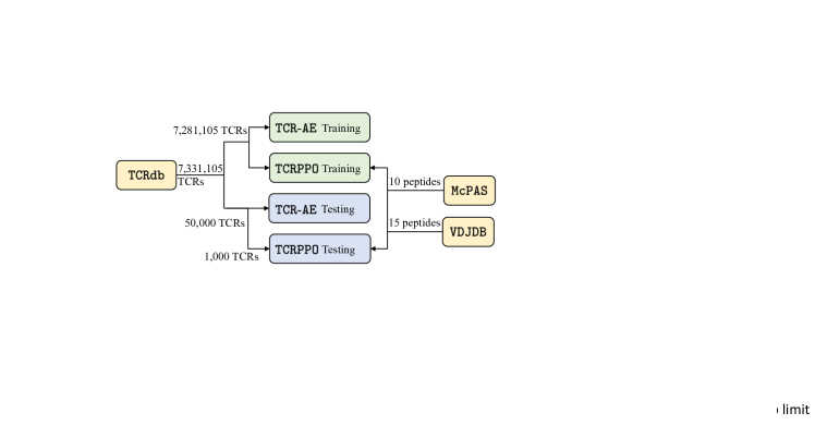
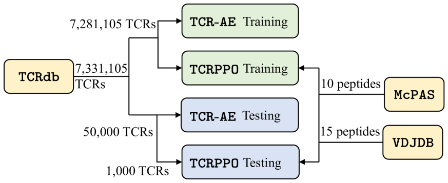
We selected peptides and TCR sequences for the training and testing of and . Figure 2 summaries the peptides and TCRs used in our experiments.
4.1.1 Peptides
To test , we first identified a set of peptides that needs to optimize TCR sequences for. We aimed at selecting the peptides which are very likely to have reliable peptide-TCR binding predictions, such that their binding predictions can serve to test ’s optimized TCRs against the respective peptides. We identified such peptides from two databases: [34] and [30], which have experimentally validated TCR-peptide binding pairs. We applied the autoencoder-based models [33] on and ( and have pre-specified training and testing sets for each peptide), and selected the peptides which have AUC values above 0.9 on their respective testing sets. This resulted in 10 peptides selected from , denoted as , and 15 peptides selected from , denoted as , with lengths ranging from 8 to 21, as presented in Appendix Table A.1. Additional discussion on peptides is available in Appendix A.1.
4.1.2 TCR sequences
We then selected TCR sequences that needs to optimize against each of the peptides selected as above. We selected such sequences from the database [6], which contains 277 million human TCR sequences, each with a TCR- sequence. Here, we used , not or , because ’s sequences are valid TCRs and have no information on their binding affinities with the selected peptides. Therefore, these valid TCRs can be used to train to calculate . Meanwhile, since is much larger than (4,528 TCRs) and (50,049 TCRs), it is very likely that the calculated from the , which is trained over data, will be independent of the calculated from , which is trained on or , avoiding possible correlation between and as in the reward (Equation 9).
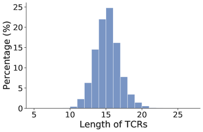
We selected all the TCRs with lengths below 27 ( can only predict sequences of length 27 or shorter) from , resulting in 7,331,105 unique TCR- sequences. Figure A.1 presents the distribution of lengths of TCRs in . As shown in Figure A.1, the most common length of TCRs is 15. Additional discussion on the length of TCRs is available in Appendix A.1. Among these selected sequences, we sampled 50K sequences, denoted as the validation set , to test and validate ; within these 50K sequences, we again sampled 1K sequences, denoted as the testing set , to test performance once it is well trained. The remaining selected sequences (i.e., not in the validation set), denoted as the training set , are used to train ; they are also used to train .
4.2 Experimental Setup
For all the selected peptides from a same database (i.e., 10 peptides from , 15 peptides from ), we trained one agent, which optimizes the training sequences (i.e., 7,281,105 TCRs in Figure 2) to be qualified against one of the selected peptides. The model trained on the corresponding database (the same model also used to select the peptides from the database as in Section 4.1) will be used to test recognition probabilities for the agent. Please note that as in Springer et al. [33], one model is trained for all the peptides in each database (i.e., one predicts TCR-peptide binding for multiple peptides). Thus, the model is suitable to test for multiple peptides in our setting. Also note that we trained one agent corresponding to each database, because peptides and TCRs in these two databases are very different, demonstrated by the inferior performance of an trained over the two databases together, and discussed in Springer et al. [33].
mutates each sequence up to 8 steps (i.e., T=8). In training, an initial TCR sequence (i.e., in ) is randomly sampled from , and will be mutated in the following states; a peptide is randomly sampled at , and remains the same in the following states (i.e., ). Once a is well trained from , it will be tested on . We set the dimensions of the hidden layers (e.g., hidden layers of action prediction networks) as 256, and the dimensions of latent embeddings (e.g., , ) as 128 (i.e., half of the hidden dimensions). Other hyper-parameters and the details of hyper-parameter selection of the TCR mutation environment, the policy network and the agent are available in Appendix A.2.
| Dataset | Method | () | () | () | () | ||||||||||||||||||
| 0.05 | 0.12 | - | 1.46 | 0.16 | 1.73 | 0.17 | 0.95 | 0.01 | 0.05 | 0.00 | 95.22 | 0.45 | 1 | ||||||||||
| 0.01 | 0.03 | - | 1.38 | 0.00 | 1.34 | 0.03 | 0.93 | 0.00 | 0.09 | 0.09 | 0.59 | 0.28 | 200 | ||||||||||
| 0.04 | 0.09 | - | 1.31 | 0.02 | 1.34 | 0.02 | 0.95 | 0.02 | 0.09 | 0.04 | 6.86 | 2.52 | 7 | ||||||||||
| (n=5) | 1.27 | 2.09 | 2.88 | 1.50 | 1.49 | 0.07 | 1.54 | 0.02 | 0.93 | 0.02 | 0.18 | 0.09 | 99.36 | 0.21 | 39 | ||||||||
| (n=10) | 2.15 | 3.86 | 3.04 | 1.48 | 1.50 | 0.11 | 1.52 | 0.02 | 0.93 | 0.02 | 0.26 | 0.11 | 99.84 | 0.12 | 77 | ||||||||
| 20.58 | 17.85 | 5.10 | 1.09 | 1.46 | 0.03 | 1.44 | 0.02 | 0.93 | 0.01 | 0.62 | 0.12 | 99.98 | 0.04 | 74 | |||||||||
| 25.18 | 21.28 | 5.16 | 1.05 | 1.46 | 0.03 | 1.46 | 0.02 | 0.93 | 0.01 | 0.69 | 0.12 | 100.00 | 0.00 | 166 | |||||||||
| 25.89 | 29.60 | 5.15 | 2.02 | 1.55 | 0.19 | 1.51 | 0.17 | 0.97 | 0.03 | 0.76 | 0.27 | 65.23 | 12.47 | 7 | |||||||||
| 36.52 | 30.25 | 5.37 | 1.81 | 1.55 | 0.17 | 1.53 | 0.17 | 0.96 | 0.03 | 0.83 | 0.21 | 75.83 | 9.46 | 7 | |||||||||
| 0.08 | 0.10 | - | 1.58 | 0.20 | 1.73 | 0.28 | 0.94 | 0.02 | 0.03 | 0.03 | 95.02 | 0.46 | 1 | ||||||||||
| 0.00 | 0.00 | - | 0.00 | 0.00 | 1.35 | 0.03 | 0.00 | 0.00 | 0.05 | 0.06 | 0.46 | 0.09 | 200 | ||||||||||
| 0.08 | 0.12 | - | 1.33 | 0.03 | 1.35 | 0.01 | 0.95 | 0.03 | 0.05 | 0.03 | 18.46 | 5.13 | 9 | ||||||||||
| (n=5) | 2.15 | 1.82 | 2.84 | 1.47 | 1.48 | 0.09 | 1.55 | 0.01 | 0.94 | 0.02 | 0.16 | 0.06 | 99.33 | 0.21 | 39 | ||||||||
| (n=10) | 4.41 | 3.72 | 3.03 | 1.52 | 1.48 | 0.07 | 1.52 | 0.02 | 0.94 | 0.01 | 0.24 | 0.08 | 99.86 | 0.08 | 77 | ||||||||
| 31.81 | 17.09 | 5.01 | 1.12 | 1.47 | 0.03 | 1.44 | 0.02 | 0.93 | 0.01 | 0.64 | 0.09 | 99.96 | 0.06 | 71 | |||||||||
| 38.57 | 20.57 | 5.07 | 1.07 | 1.48 | 0.03 | 1.47 | 0.02 | 0.94 | 0.01 | 0.72 | 0.09 | 100.00 | 0.00 | 156 | |||||||||
| 45.82 | 21.59 | 5.34 | 1.58 | 1.51 | 0.19 | 1.51 | 0.19 | 0.96 | 0.02 | 0.87 | 0.18 | 69.99 | 11.74 | 7 | |||||||||
| 58.97 | 29.11 | 5.20 | 1.69 | 1.65 | 0.20 | 1.63 | 0.19 | 0.97 | 0.02 | 0.89 | 0.17 | 82.41 | 5.54 | 6 | |||||||||
-
•
Columns represent: : the percentage of qualified TCR sequences; : the edit distance between the original TCR sequences and the mutated qualified TCR sequences; /: the average scores over the TCRs in set /; /: the average probabilities over the TCRs in set /; : the percentage of valid TCR sequences. : the average number of calls to calculate functions. Values represent mean and standard deviation . “-”: not applicable. The “" value in indicates that is done times over each sequence.
4.3 Baseline Methods
We compared the method and with multiple baseline methods of two primary categories: 1) generative methods that generate a new TCR in its entirety, and 2) mutation-based methods that optimize TCRs via mutating amino acids of existing TCRs. For generative methods, we used two baseline methods including Monte Carlo tree search () [8] and a variational autoencoder with backpropagation () [13]. For mutation-based methods, we used three baseline methods to mutate each TCR sequence up to 8 steps and stop the mutation once a qualified TCR is generated, including random mutation (), greedy mutation () and genetic mutation () [38]. In addition, we used a random selection method () as another baseline to randomly sample a TCR from , which helps quantify the space of valid TCRs. More details about baseline methods are available in Appendix A.3.
4.4 Evaluation Metrics
We evaluated all the methods using six metrics including: (1) qualification rate , which measures the percentage of qualified TCRs (Section 3.1) among all the output TCRs; (2) edit distance between and (), which measures sequence difference between and qualified ; (3) average TCR validity score over valid TCRs or over qualified TCRs; (4) average recognition probability over valid TCRs or over qualified TCRs; (5) validity rate , which measures the percentage of valid TCRs (Section 3.1) among all the output TCRs; (6) average number of calls to calculation () (Equation 9) over all the generated TCRs, which estimates the efficiency of methods. We calculated the metrics over two different sets of output TCRs: (1) the set of valid TCRs : ; (2) the set of qualified TCRs : .
5 Experimental Results
5.1 Comparison on TCR Optimization Methods
5.1.1 Overall Comparison
Table 1 presents the overall comparison among all the methods over and . In , methods achieve overall the best performance: in terms of , achieves , which slightly outperforms the best from the baseline method (). achieves the best at among all the methods, which is 45.04% better than the best from the baseline methods ( from ). achieves so with a few calls ( =7). In , methods also achieve overall the best performance: in terms of , and outperform the best baseline by 18.80% and 52.89%.
Among the qualified TCRs () for , and methods achieve the highest values on average ( for ; for ), with above 6% improvement from those of , which achieves the best among all the baseline methods. Note that qualified TCRs must have above , which is set as 1.2577 as discussed in Appendix A.4.4. The significant high values from methods demonstrate that is able to generate qualified TCRs that are highly likely to be valid TCRs. In terms of among qualified TCRs, methods have value , above the . Note that , a very high threshold for to determine TCR-peptide binding, is actually a very tough constraint. The fact that methods can survive this constraint with substantially high and highly likely valid TCRs as results demonstrates the strong capability of methods. In addition, methods need a few number of calls to calculate (i.e., 7 for , compared to 166 for ), indicating that is very efficient in identifying qualified TCRs. In , we observed very similar trends as those in .
Among all the baseline methods, randomly selects a valid TCR from , given that some TCRs in may already qualify. Thus, it is a naive baseline for all the other methods. It has around 95%, corresponding to how our threshold is identified (by 95 percentile true positive rate) as discussed in Appendix A.4.4. On average, among all valid TCRs, about 0.05% ( in ) TCRs are qualified TCRs. , , and methods substantially outperform this baseline method.
5.1.2 Comparison among Mutation-based Methods
, , , and are mutation-based methods: they start from a valid TCR from , and optimize the TCR by mutating its amino acids. Among all the mutation-based methods, and outperform others as discussed above. Below we only focused on , as similar trends exist on .
In , underperforms all the other mutation-based methods: it has below 3% on average, but has very high (close to 100%). uses to select randomly mutated sequences, which decomposes to its and its components. starts from valid TCRs with high already, but low in general. During random mutation, cannot be easily improved as no knowledge or informed guidance is used to direct the mutation towards better . Therefore, the component in will dominate, leading to that the final selected, best mutated sequence tends to have high to satisfy high . Such best mutated sequence tends to occur after only a few random mutations, since as shown in Appendix A.4.4, random mutations can quickly decrease values. Thus, the qualified sequences produced from tend to be more similar to the initial TCRs ( is small, around 3; high as ), their values are high (close to 1.5; highest among all mutation-based methods) but is low due to hardly improved values.
In , has a better () than and also a high (). leverages a greedy strategy to select the random mutation that gives the best at the current step. Thus, it leverages some guidance on improvement based on , and can improve values compared to . As in Table 1, it has better value () for valid TCRs. Meanwhile, explores a large sequence space, allowing its to identify more valid TCRs, leading to high (), high (; also due to better improvement) but more diverse results () than .
is the second best mutation-based method on , after methods. explores a sequence space even larger than that in , and uses to guide next mutations also in a greedy way. Thus, it enjoys the opportunity to reach more, potentially qualified TCRs, demonstrated by high () indicating diverse sequences, and thus achieves a better () than , even better than that of , and a high (), at a significant cost of many more calls to calculate . Even though, it still significantly underperforms in terms of and qualities of qualified TCRs as discussed earlier.
5.1.3 Comparison between Mutation-based Methods and Generation-based Methods
Overall, mutation-based methods substantially outperform generation-based methods. For example, in terms of , mutation-based methods (excluding random mutation ) has an average in , compared to of the generation-based methods ( and ). In addition to the superior performance, mutation-based methods have strong biological relevance that make them very suitable and practical for TCR-T based precision immunotherapy, in which they can be readily employed to optimize existing TCRs found in patient’s TCR repertoire. However, any promising TCRs generated from generation-based methods have to be either synthesized, which could be both very costly and technically challenging, or mutated from existing TCRs that are similar to the generated TCRs in their amino acids. Detailed discussions on generation-based methods are available in Appendix A.4.1.
5.2 Evaluation on Optimized TCR Sequences
[] \sidesubfloat[]
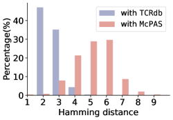
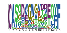
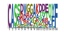
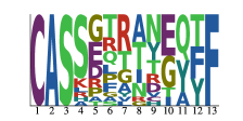
Figure 3A presents the entropy of amino acid distributions at each sequence position among the length-15 TCRs for each peptide. Here the TCRs are optimized by with respect to the peptides. Figure 3A clearly shows some common patterns among all the optimized TCRs. For example, the first three positions and last four positions tend to have high conservation. TCRs for some peptides (e.g., “SSPPMFRV", “ASNENMETM", and “RFYKTLRAEQASQ") have high variations at internal regions. Similar patterns are also observed among the binding TCRs for other peptides in 222https://vdjdb.cdr3.net/motif.
Figure 3B presents the difference between qualified TCRs optimized by and existing TCRs. It presents the distribution of Hamming distances between qualified TCRs (length 15) for peptide “RFYKTLRAEQASQ” and their most similar (in terms of Hamming distance) TCRs that are known to bind to this peptide in ; and the distribution of Hamming distances between qualified TCRs for this peptide and their most similar TCRs in . This figure demonstrates that the qualified TCRs by are actually different from known binding TCRs, but there are TCRs similar to them existing in . This can be meaningful for precision immunotherapy, as can produce diverse TCR candidates that are different from known TCRs, leading to a novel sequence space; meanwhile, these TCR candidates actually have similar human TCRs available for further medical evaluation and investigation purposes.
Additional analyses are available in Appendix A.4, such as the overview of amino acid distributions of TCRs, the patterns for binding TCRs and the comparison on TCR detection. Specifically, we found that can successfully learn the patterns of TCRs (Appendix A.4.2); we also found that can identify the specific binding patterns which are more conserved than the real binding patterns (Appendix A.4.3). We also found that our scoring method successfully distinguishes TCRs from non-TCRs in Appendix A.4.4.
6 Conclusions and Outlook
In this paper, we presented a reinforcement learning framework to optimize TCRs for more effective TCR recognition, which has the potential to guide TCR engineering therapy. Our experimental results in comparison with generation-based methods and mutation-based methods on optimizing TCRs demonstrate that outperforms the baseline methods. Our analysis on the TCRs generated by demonstrates that can successfully learn the conservation patterns of TCRs. Our experiments on the comparison between the generated TCRs and existing TCRs demonstrate that can generate TCRs similar to existing human TCRs, which can be used for further medical evaluation and investigation. Our results in TCR detection comparison show that the score in our framework can very effectively detect non-TCR sequences. Our analysis on the distribution of scores over mutations demonstrates that mutates sequences along the trajectories not far away from valid TCRs.
Our proposed is a modular and flexible framework. Thus, the and scoring functions in the reward design can be replaced with other predictors trained on large-scale data when available. Also, can be further improved from the following perspectives. First, the recognition probabilities of TCRs considered in our paper are based on a peptide-TCR binding predictor (i.e., ) rather than experimental validation. Therefore, testing the generated qualified TCR candidates in a wet-lab will be needed ultimately to validate the interactions between TCRs and peptides. Moreover, when the predicted recognition probabilities are not sufficiently accurate, learned from unreliable rewards could be inaccurate, resulting in generating TCRs that could not recognize the given peptide. Thus, it could be an interesting and challenging future work to incorporate the reliabilities of predictions in the reward function of , so that the effect of unreliable recognition probabilities can be alleviated. Finally, only considers the CDR3 of chain in TCRs, while other regions of TCRs, though not contributing most to interactions between TCRs and peptides, are not considered. In this sense, incorporating other regions of TCRs (e.g., CDR3 of alpha chains) could be an interesting future work.
References
- [1] Abati, D., Porrello, A., Calderara, S., Cucchiara, R.: Latent space autoregression for novelty detection. In: Proceedings of the IEEE/CVF Conference on Computer Vision and Pattern Recognition (CVPR) (June 2019)
- [2] Angermüller, C., Dohan, D., Belanger, D., Deshpande, R., Murphy, K., Colwell, L.: Model-based reinforcement learning for biological sequence design. In: 8th International Conference on Learning Representations, ICLR 2020, Addis Ababa, Ethiopia, April 26-30, 2020 (2020)
- [3] Arnold, F.H.: Design by directed evolution. Accounts of Chemical Research 31(3), 125–131 (feb 1998)
- [4] Auer, P., Cesa-Bianchi, N., Fischer, P.: Machine Learning 47(2/3), 235–256 (2002)
- [5] Cai, M., Bang, S., Zhang, P., Lee, H.: ATM-TCR: TCR-epitope binding affinity prediction using a multi-head self-attention model. Frontiers in Immunology 13 (jul 2022)
- [6] Chen, S.Y., Yue, T., Lei, Q., Guo, A.Y.: TCRdb: a comprehensive database for t-cell receptor sequences with powerful search function. Nucleic Acids Research 49(D1), D468–D474 (sep 2020)
- [7] Chen, Z., Min, M.R., Ning, X.: Ranking-based convolutional neural network models for peptide-MHC class i binding prediction. Frontiers in Molecular Biosciences 8 (may 2021)
- [8] Coulom, R.: Efficient selectivity and backup operators in monte-carlo tree search. In: Computers and Games, pp. 72–83. Springer Berlin Heidelberg (2007)
- [9] Craiu, A., Akopian, T., Goldberg, A., Rock, K.L.: Two distinct proteolytic processes in the generation of a major histocompatibility complex class i-presented peptide. Proceedings of the National Academy of Sciences 94(20), 10850–10855 (sep 1997)
- [10] Esfahani, K., Roudaia, L., Buhlaiga, N., Rincon, S.D., Papneja, N., Miller, W.: A review of cancer immunotherapy: From the past, to the present, to the future. Current Oncology 27(12), 87–97 (apr 2020)
- [11] Freeman, J.D., Warren, R.L., Webb, J.R., Nelson, B.H., Holt, R.A.: Profiling the t-cell receptor beta-chain repertoire by massively parallel sequencing. Genome Research 19(10), 1817–1824 (jun 2009)
- [12] Glanville, J., Huang, H., Nau, A., Hatton, O., Wagar, L.E., Rubelt, F., Ji, X., Han, A., Krams, S.M., Pettus, C., et al.: Identifying specificity groups in the t cell receptor repertoire. Nature 547(7661), 94–98 (2017)
- [13] Gómez-Bombarelli, R., Wei, J.N., Duvenaud, D., Hernández-Lobato, J.M., Sánchez-Lengeling, B., Sheberla, D., Aguilera-Iparraguirre, J., Hirzel, T.D., Adams, R.P., Aspuru-Guzik, A.: Automatic chemical design using a data-driven continuous representation of molecules. ACS Central Science 4(2), 268–276 (jan 2018)
- [14] González, J., Longworth, J., James, D.C., Lawrence, N.D.: Bayesian optimization for synthetic gene design (2015)
- [15] Graves, A., Schmidhuber, J.: Framewise phoneme classification with bidirectional LSTM and other neural network architectures. Neural Networks 18(5-6), 602–610 (jul 2005)
- [16] Gupta, A., Zou, J.: Feedback GAN for DNA optimizes protein functions. Nature Machine Intelligence 1(2), 105–111 (feb 2019)
- [17] Hinton, G.E., Vinyals, O., Dean, J.: Distilling the knowledge in a neural network. CoRR abs/1503.02531 (2015)
- [18] Hou, X., Wang, M., Lu, C., Xie, Q., Cui, G., Chen, J., Du, Y., Dai, Y., Diao, H.: Analysis of the repertoire features of TCR beta chain CDR3 in human by high-throughput sequencing. Cellular Physiology and Biochemistry 39(2), 651–667 (2016)
- [19] Killoran, N., Lee, L.J., Delong, A., Duvenaud, D., Frey, B.J.: Generating and designing DNA with deep generative models. CoRR abs/1712.06148 (2017)
- [20] La Gruta, N.L., Gras, S., Daley, S.R., Thomas, P.G., Rossjohn, J.: Understanding the drivers of mhc restriction of t cell receptors. Nature Reviews Immunology 18(7), 467–478 (2018)
- [21] Mnih, V., Badia, A.P., Mirza, M., Graves, A., Lillicrap, T., Harley, T., Silver, D., Kavukcuoglu, K.: Asynchronous methods for deep reinforcement learning. In: Proceedings of The 33rd International Conference on Machine Learning. vol. 48, pp. 1928–1937. PMLR, New York, New York, USA (20–22 Jun 2016)
- [22] Pang, G., Shen, C., Cao, L., Hengel, A.V.D.: Deep learning for anomaly detection: A review. ACM Comput. Surv. 54(2) (mar 2021)
- [23] Platt, J.: Probabilistic outputs for support vector machines and comparisons to regularized likelihood methods. Advances in large margin classifiers 10(3), 61–74 (mar 1999)
- [24] Raffin, A., Hill, A., Gleave, A., Kanervisto, A., Ernestus, M., Dormann, N.: Stable-baselines3: Reliable reinforcement learning implementations. Journal of Machine Learning Research 22(268), 1–8 (2021)
- [25] Ren, J., Liu, P.J., Fertig, E., Snoek, J., Poplin, R., DePristo, M.A., Dillon, J.V., Lakshminarayanan, B.: Likelihood Ratios for Out-of-Distribution Detection. Curran Associates Inc., Red Hook, NY, USA (2019)
- [26] Rossjohn, J., Gras, S., Miles, J.J., Turner, S.J., Godfrey, D.I., McCluskey, J.: T cell antigen receptor recognition of antigen-presenting molecules. Annual review of immunology 33, 169–200 (2015)
- [27] Sadelain, M., Rivière, I., Riddell, S.: Therapeutic t cell engineering. Nature 545(7655), 423–431 (2017)
- [28] Schulman, J., Moritz, P., Levine, S., Jordan, M., Abbeel, P.: High-dimensional continuous control using generalized advantage estimation. In: Proceedings of the International Conference on Learning Representations (ICLR) (2016)
- [29] Schulman, J., Wolski, F., Dhariwal, P., Radford, A., Klimov, O.: Proximal policy optimization algorithms. CoRR abs/1707.06347 (2017)
- [30] Shugay, M., Bagaev, D.V., Zvyagin, I.V., Vroomans, R.M., Crawford, J.C., Dolton, G., et al.: VDJdb: a curated database of t-cell receptor sequences with known antigen specificity. Nucleic Acids Research 46(D1), D419–D427 (sep 2017)
- [31] Skwark, M.J., Carranza, N.L., Pierrot, T., Phillips, J., Said, S., Laterre, A., Kerkeni, A., Sahin, U., Beguir, K.: Designing a prospective COVID-19 therapeutic with reinforcement learning. CoRR abs/2012.01736 (2020)
- [32] Snover, M., Dorr, B., Schwartz, R., Micciulla, L., Makhoul, J.: A study of translation edit rate with targeted human annotation. In: Proceedings of the 7th Conference of the Association for Machine Translation in the Americas: Technical Papers. pp. 223–231. Cambridge, Massachusetts, USA (Aug 8-12 2006)
- [33] Springer, I., Besser, H., Tickotsky-Moskovitz, N., Dvorkin, S., Louzoun, Y.: Prediction of specific TCR-peptide binding from large dictionaries of TCR-peptide pairs. Frontiers in Immunology 11 (aug 2020)
- [34] Tickotsky, N., Sagiv, T., Prilusky, J., Shifrut, E., Friedman, N.: McPAS-TCR: a manually curated catalogue of pathology-associated t cell receptor sequences. Bioinformatics 33(18), 2924–2929 (may 2017)
- [35] Verdegaal, E.M.E., de Miranda, N.F.C.C., Visser, M., Harryvan, T., van Buuren, M.M., Andersen, R.S., Hadrup, S.R., van der Minne, C.E., Schotte, R., Spits, H., Haanen, J.B.A.G., Kapiteijn, E.H.W., Schumacher, T.N., van der Burg, S.H.: Neoantigen landscape dynamics during human melanoma–t cell interactions. Nature 536(7614), 91–95 (jun 2016)
- [36] Waldman, A.D., Fritz, J.M., Lenardo, M.J.: A guide to cancer immunotherapy: from t cell basic science to clinical practice. Nature Reviews Immunology 20(11), 651–668 (may 2020)
- [37] Weber, A., Born, J., Martínez, M.R.: TITAN: T-cell receptor specificity prediction with bimodal attention networks. Bioinformatics 37(Supplement_1), i237–i244 (jul 2021)
- [38] Whitley, D.: A genetic algorithm tutorial. Statistics and Computing 4(2) (jun 1994)
- [39] Williams, R.J., Zipser, D.: A learning algorithm for continually running fully recurrent neural networks. Neural Computation 1(2), 270–280 (jun 1989)
- [40] Zong, B., Song, Q., Min, M.R., Cheng, W., Lumezanu, C., Cho, D., Chen, H.: Deep autoencoding gaussian mixture model for unsupervised anomaly detection. In: International Conference on Learning Representations (2018)
A.1 Data Analyses
We listed the selected peptides from and in Table A.1. As shown in Table A.1, these selected peptides are very different. For example, the average edit distance between pairs of peptides in and are 10.84 and 9.14, respectively, demonstrating the diversity of peptides compared with the average length of peptides in and (10.90 and 9.67). Comparing with , we found that 6 peptides included in are also included in , which could be due to the data overlapping between and [30].
We also listed the distribution of length of TCRs in in Figure A.1. We found that the most common length of TCRs is 15; and TCRs with 13, 14, 15, and 16 lengths account for over 10% of the entire database. In this manuscript, our analyses focus on TCRs of length 13, 14, 15 and 16.
| ASNENMETM | ASNENMETM | |
| ATDALMTGY | ATDALMTGY | |
| HGIRNASFI | CTPYDINQM | |
| HPKVSSEVHI | FPRPWLHGL | |
| MEVGWYRSPFSRVVHLYRNGK | FRDYVDRFYKTLRAEQASQE | |
| RFYKTLRAEQASQ | GTSGSPIVNR | |
| SSLENFRAYV | HGIRNASFI | |
| SSPPMFRV | LSLRNPILV | |
| SSYRRPVGI | NAITNAKII | |
| YSEHPTFTSQY | SQLLNAKYL | |
| SSLENFRAYV | ||
| SSPPMFRV | ||
| SSYRRPVGI | ||
| STPESANL | ||
| TTPESANL |
A.2 Parameter setup
| description | value |
|---|---|
| maximum steps | 8 |
| threshold of | 0.9 |
| threshold of | 1.2577 |
| discount factor | 0.9 |
| latent dimension of | 256 |
| hidden dimension of policy & value networks | 128 |
| hidden layers of policy & value networks | 2 |
| number of steps per iteration | 5,120 |
| batch size for policy update | 64 |
| number of epochs per iteration | 10 |
| clip range | 0.2 |
| learning rate | 3e-4 |
| coefficient for value function | 0.5 |
| coefficient for entropy regularization | 0.01 |
We listed the hyper-parameters of the TCR mutation environment, the policy network and the agent in Table A.2. We selected an optimal set of hyperparameters including the discount factor, the entropy coefficient and the maximum steps by a grid search, according to the average rewards of the final 10 iterations. Particularly, we set the maximum steps as 8 steps, as we empirically found that it can lead to the highest average final rewards. We set the parameter as 0.5 for the tradeoff between validity scores and recognition probabilities, as we empirically found that different values could lead to comparable results. We also constructed a validation set by sampling 1,000 TCRs from the test set of ; these TCRs are not included in the test set of . We then selected the hyperparameters including the hidden dimension of policy network and value networks and the ratio of difficult initial state from that the corresponding models achieve the maximum qualified percentage . Among three options , the optimal hidden dimensions of policy and value networks for and are 128. We set the latent dimension of to be double of the optimal hidden dimensions, that is, 256. In terms of encodings of amino acids, we set the dimension of learnable embeddings as 20, which is the same with the dimensions of BLOSUM embeddings and one-hot encodings; that is, the total dimension of amino acid encodings is 60. In terms of ratios of difficult initial state, the optimal ratios for and are 0.2 and 0.1, respectively. We set the threshold for recognition probability as 0.9, which is demonstrated as a proper threshold as it can lead to 47.04% and 56.48% at true positive rate and 0.16% and 0.30% at false positive rate, respectively, for selected peptides in and . In the implementation of , for each iteration, we ran 20 environments in parallel for 256 timesteps and collect trajectories with 5,120 timesteps in total. We trained for 1e7 timesteps (i.e., 1954 iterations). We set all the other hyper-parameters for the agent as the default hyper-parameters provided by the stable-baselines3 [24], as we found little performance improvement from tuning these parameters. We trained the models using a Tesla P100 GPU and a CPU on Red Hat Enterprise 7.7. It took 9-10 hours to train a model. With the trained model available, on a single GPU and a single CPU core, optimizing 1,000 TCRs for a single peptide using takes 160.5 seconds, which is faster than that of the state-of-the-art baseline (i.e., 207.8s).
For , we selected an optimal set of hyperparameters including the dimension of hidden layers and the dimension of latent layers. According to the reconstruction accuracy on the validation set, we set the dimension of hidden layers in to be 64, and the dimension of latent layers to be 16. At each step, we randomly sampled 256 TCR sequences from , and trained the for 100,000 steps. This is with high reconstruction accuracy on our validation set, which is %, and thus can be used to provide reliable reconstruction-based scores for TCR sequences.
A.3 Baseline methods
We describe the baseline methods used in the main text as follows,
-
•
: Monte Carlo Tree Search. Given a peptide , generates TCR sequences by adding one amino acid step by step until reaching the maximum length of 20 amino acids or with the recognition probability greater than . All the generated peptides with no less than 10 amino acids will be evaluated by . The approach of is described in Algorithm A.1. At each step, the amino acid to be added is determined by the Upper Confidence Bound algorithm (see equation in line 12 of Algorithm A.1) to balance exploration and exploitation [4]. The hyper-parameter is set as 0.5. For each peptide, the number of rollout is set as 1,000, as all the methods including generate 1,000 TCRs for each peptide. At the beginning of search, we initialize the sequence with “C”, as all the TCRs in begin with “C”. We collected all the generated TCRs during the search process, and calculated the metrics listed in Table 1 over the 1,000 TCRs with the highest reward values for each peptide.
-
•
: Back Propagation with the Variational Autoencoder. In , a VAE model is first pre-trained to convert TCR sequences of variable lengths into continuous latent embeddings of a fixed size with a single-layer LSTM. Then, a student model with the pre-trained VAE is employed to distill knowledge from via learning the recognition probabilities produced by from the latent embeddings [17]. Note that during this fine-tuning process, the parameters of pre-trained VAE will also be updated. With the well-trained student model, can generate TCRs by optimizing the latent embeddings of TCRs through gradient ascent to maximize the predicted recognition probabilities from the student model. The decoded TCR sequences with the prediction from student model greater than will be evaluated by function. We fine-tuned the hyper-parameters and set the dimension of hidden layers for VAE as 64, the dimension of latent embeddings as 8, the batch size as 256, the initial coefficient for KL loss as 0.05 and the initial learning rate as 0.005. We increased the coefficient by 0.05 every 1e4 steps until reaching the maximum coefficient limit 0.3; we also decreased the learning rate by 10 percent every 5,000 steps until reaching the minimum learning rate limit 0.0001. We pre-trained the VAE model for 2e6 steps. We then fine-tune the VAE model with the student model for 50,000 steps. During the inference, we set the maximum step for gradient ascent as 50 and the learning rate of gradient ascent as 0.05. Similar to , we collected all the generated TCRs and calculated the metrics over the 1,000 TCRs with the highest reward values for each peptides.
-
•
: random mutation. It randomly mutates a sequence one amino acid at a step up to 8 steps, each step leading to an intermediate mutated sequence; it does so for each sequence times, generating 8 mutated sequences. It selects the mutated sequence with the highest as the final output.
-
•
: greedy mutation. It randomly mutates one amino acid of at step , and does this 10 times, generating 10 mutated sequences which are all one-amino-acid different from . It selects the one with best among the 10 sequences as the next sequence to further mutate.
-
•
: genetic mutation. It randomly mutates each sequence in the population (size ) five times, each at one site, generating five mutated sequences. Among all the mutated sequences for all the sequences in the population, selects the top- sequences with the best as the next population.
A.4 Additional Results
A.4.1 Discussion on Comparison among Generation-based Methods
Generation-based methods and on average very much underperform mutation-based methods. Both and hardly generate any qualified TCRs (very low : for and for in ). explores potentially the entire sequence space, including both valid TCRs and non-TCRs. Although it uses to guide the search, with substantially more calls to calculate than other methods, due to the fact that valid TCRs may only occupy an extreme small portion of the entire sequence space, it is extremely challenging for to find qualified TCRs. In , even cannot find any qualified TCR for all the peptides within 1,000 rollouts, and thus has zero values at and . An estimation using over all possible length-15 sequence space results at most % TCRs being valid in the sequence space. Therefore, it is possible that ends at a region in the sequence space with even worse than random selection method .
Similarly, also has a minimum (). encodes valid TCRs into its latent space, and uses a predictor in the latent space, which is trained to approximate , to guide the search of an optimal latent vector. This vector could correspond to a binding TCR and then is decoded to a TCR sequence. However, there is a phenomenon that is observed in other VAE-based generative approaches [13]: while the latent vector is searched under a guidance to maximize desired properties, its decoded instance does not always have the properties or are not even valid. This phenomenon also appears in : the decoded TCRs are not qualified most of the times. This might be due to the propagation or magnification of the errors from the predictor in the latent space, or the exploration in the latent space ends at a region far away from that of valid TCRs. However, theoretical justification behind VAE-based generative approaches is out of the scope of this paper.
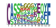
A.4.2 Overview of Amino Acid Distributions of TCRs
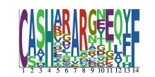
Valid TCRs, regardless of their binding affinities against any peptides, have certain patterns [11]. For example, the first and last amino acids have to be ‘C’ and ‘F’, respectively. Figure A.2 presents the patterns among different TCRs of length 13, 14, 15 and 16. For TCRs of length 15 (most common TCR length), the left panel of Figure A.2 shows the enrichment of different amino acids at different positions among peptides in . Recall that has 277 million valid human TCRs, and thus the patterns in the left panel of Figure A.2 are very representative of the common patterns among valid TCRs. The middle panel of Figure A.2 shows that the patterns among the TCRs that produces for peptides in are similar to those of TCRs in . For example, ‘G’ is one of the most frequent amino acids on positions 6-9; the first three positions and the last four positions of optimized TCRs have patterns highly similar to those in TCRs. Similar observations are also for the TCRs that produces for peptides in as in the right panel of Figure A.2. Please note that in , we do not impose any rules to reserve amino acids at the ends of sequences when generating TCRs with both high validity and high recognition probability against given peptides; clearly, successfully learns the pattern. In Figure A.2, A.2 and A.2, the same observations are for TCRs of length 13, 14 and 16 as in Figure A.2 for TCRs of length 15. For example, the first three positions and the last three positions of generated TCRs have very similar patterns with those in (i.e., dominated by “CAS” and “QYF”). This indicates that also successfully learn the patterns for TCRs of other lengths.
[]


\sidesubfloat[]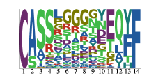

\sidesubfloat[]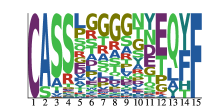


\sidesubfloat[]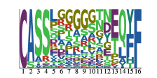
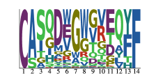
A.4.3 Amino Acid Distributions of Binding TCRs
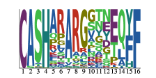
Figure A.3 presents the patterns among binding TCRs in dataset (left) and the generated TCRs of different lengths for peptide “RFYKTLRAEQASQ” in . Particularly, as in Figure A.3, the patterns among binding TCRs in are similar to those of generated TCRs. For example, the most frequent amino acids at position 6 - 9 in generated TCRs (i.e., “R”, “A”, “R”, “G”) are also one of the most frequent amino acids at corresponding positions in known binding TCRs. Similar observations are also for generated TCRs of different lengths. This demonstrates that can successfully identify the patterns of binding TCRs. In addition to the similar patterns, we also observe the inconsistent patterns between known binding TCRs and generated TCRs. For example, the generated TCRs are highly conserved on position 4, that is, most fourth amino acids are “H”; this conservation pattern does not exist in known binding TCRs. Please note that “H” also exists on position 4 among known binding TCRs as in Figure A.3. One reason for inconsistency between generated TCRs and known binding TCRs could be that only limited percentage of binding TCRs are with predicted recognition probabilities greater than 0.9, resulting in that generated TCRs are more conserved on some patterns.
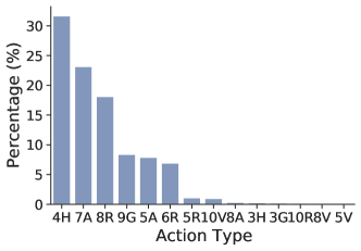
Figure A.4 presents the distribution of action types produced by for TCRs of length 15 binding to the peptide “RFYKTLRAEQASQ”. As shown in Figure A.4, positions 5, 7, 9 in the TCRs prefer to be Histidine (“H”), Alanine (“A”), Arginine(“R”) and Glycine (“G”). Since Alanine and Glycine are non-polar and hydrophobic, the hydrophobic effect tends to be strong around these positions. On the other hand, position 4 prefer to be Histidine, which has a positive charge on its side chain. Additionally, positions 5, 6, 8 in the TCRs prefer to be Arginine, which is hydrophilic and has a positive charge on its side chain. This shows that the binding pocket around these positions is more electrophilic which favors the interaction with amino acids with positive charges.
[]

\sidesubfloat[]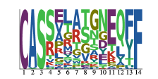
\sidesubfloat[]

\sidesubfloat[]
A.4.4 Comparison on TCR Detection
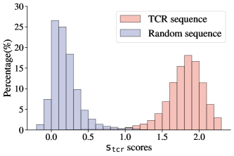
We compared our scoring method (Equation 8) and the likelihood ratio method [25], denoted as , on distinguishing TCRs from non-TCRs. The likelihood ratio method is one of the state-of-the-art methods on out-of-distribution (OOD) detection for genomic sequences. To compare and , we generated 50,000 sequences for each TCR in , with the two ends conserved to ‘C’ and ‘F’ respectively as in valid TCRs, and all the other internal amino acids fully random. These generated, random sequences will be considered as non-TCRs. The conserved ‘C’ and ‘F’ ends among the non-TCRs ensure that they are not trivially separable from TCRs simply due to the ends. We compared and scores to detect TCRs from such non-TCRs, and present their distributions in Figure A.5.
[] \sidesubfloat[]
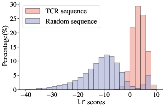
[] \sidesubfloat[]
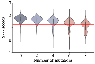
Figure A.5A shows that TCRs and non-TCRs are well separated by their scores, while Figure A.5B shows a clear overlap between TCRs and non-TCRs using their scores. Using the 5 percentile of scores on TCRs, corresponding to value 1.2577 and 95% true positive rate on TCRs, as the decision boundary, scoring method achieves 0.10% false positive rate. Using the 5 percentile of scores on TCRs (corresponding to ), has a much higher false positive rate 8.26%. This demonstrates that is very effective in distinguishing TCRs. Please note that the random sequences are not guaranteed to be true non-TCRs. However, given the random nature of these sequences, it is highly likely that they are not valid TCRs. In , we used 1.2577 as the threshold to quantify if a sequence is a valid TCR (i.e., ).
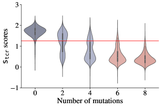
Figure A.6 presents the change of scores over mutations. Figure A.6A shows that as TCRs have more random mutations, their scores decrease dramatically. This implies that the TCR optimization via mutation is not trivial, as a random/bad mutation can significantly decrease score and easily lead to an unqualified solution. However, as Figure A.6B shows, the scores do not decrease very dramatically during mutations, consistently with a good portion of mutated sequences being valid TCRs. This demonstrates that for this non-trivial optimization problem, succeeds in mutating sequences along the trajectories not far away from valid TCRs, toward final qualified sequences.