Theory of the low- and high-field superconducting phases of UTe₂

Abstract

Recent nuclear magnetic resonance (NMR) and calorimetric experiments have observed that UTe₂ exhibits a transition between two distinct superconducting phases as a function of magnetic field strength for a field applied along the crystalline $b$-axis. To determine the nature of these phases, we employ a microscopic two-band minimal Hamiltonian with the essential crystal symmetries and structural details. We also adopt anisotropic ferromagnetic exchange terms. We study the resulting pairing symmetries and properties of these low- and high-field phases in mean field theory.

I Introduction

The material UTe₂ Ran et al. (2019) has been the subject of extensive recent investigation due to its multifarious manifestations of exotic superconductivity. The upper critical field along the crystalline $b$ axis, $H_{c}=40\text{ T}$Ran et al. (2019); Helm et al. (2022), is strikingly large in light of the critical temperature $T_{c}=1.6\text{ K}$, and is indicative of an odd parity superconducting ground state. UTe₂ belongs to a larger family of uranium-based candidate unconventional superconductors, the rest of which exhibit ferromagnetism coexisting with superconductivity Saxena et al. (2000); Aoki et al. (2001); Huy et al. (2007); Aoki and Flouquet (2012). In contrast, UTe₂ lacks magnetic order Ran et al. (2019). Thus, UTe₂ offers the opportunity to probe unconventional superconductivity in a family of materials without the confounding effects of magnetism. Furthermore, UTe₂ is also believed to host exotic phenomena such as reentrant superconductivityRan et al. (2019); Knebel et al. (2019), broken time-reversal symmetry Jiao et al. (2020); Hayes et al. (2021), and pair density wave (PDW) order Gu et al. (2022), thus positioning it as a paradigmatic unconventional superconductor.

Like the other uranium-based superconductors, UTe₂ exhibits reentrant superconductivity as a function of the strength of the magnetic field applied along the crystalline $b$ axis. While this phenomenon was initially attributed to fluctuations near a ferromagnetic quantum critical point, a few studiesYu and Raghu (2022); Ishizuka et al. (2019) offered an alternative explanation: distinct superconducting phases at low and high magnetic field strengths.

Recent experiments Kinjo et al. (2022); Rosuel et al. (2022) have confirmed the existence of two distinct superconducting phases in UTe₂, distinguished primarily by their responses to the orientation of the applied magnetic field. The state at low magnetic field strengths has little sensitivity to the direction of the field. In contrast, the superconducting state at high magnetic field strengths is easily suppressed by tilting the field away from the $b$ axis in either the $a$ or $c$ directionsKinjo et al. (2022); Rosuel et al. (2022); Knebel et al. (2019). Thus, a fundamental question regarding the unconventional superconductivity in UTe₂ is: What are the pairing symmetries associated with these superconducting phases?

In this work, we provide concrete predictions for the pairing symmetries of the low- and high-field superconducting phases. As we describe in Sec. III, we do this in two ways. In both, we use a minimal Hamiltonian with the essential symmetries and structural details, including spin-orbit coupling. First, we calculate the pair field susceptibility $\chi$, which is defined in Sec. III.1. This reveals the dominant superconducting tendencies of the normal state as determined by the kinetic energy. Second, we introduce local, anisotropic ferromagnetic pairing interactions and solve the self-consistent mean-field gap equation with these interactions (Sec. III.2). In both approaches, we find that the low- and high-field superconducting states are odd-parity states, but with the spin pointing in different primary directions. At small magnetic field strengths, the pairing state has spin predominantly in the $ac$ plane, but at high enough magnetic field strengths, this spin aligns with the $b$ axis. The change in pairing symmetry also has consequences for the physical properties of the state. In Sec. IV, we infer the nodal structure of the gap from our results and discuss the properties of the phases.

II Model

In this section, we describe the tight-binding Hamiltonian used throughout this work and the symmetry classifications of the allowed pairing states. The main assumption in our work is that the fermions relevant for superconductivity reside on uranium atoms, which is reflected in the pairing symmetry classifications and the minimal Hamiltonian.

Theoretical predictions for the density of states in UTe₂ find that uranium $5f$ orbitals contribute the largest density of states at the Fermi energy Fujimori et al. (2021), so the uranium electrons are likely the driver of superconductivity in the system. The rung (sublattice) structure is also believed to play a crucial role in determining the electronic and superconducting properties of the materialXu et al. (2019); Shishidou et al. (2021); Hazra and Coleman (2022). Thus, we anticipate that the superconducting properties of UTe₂, including the symmetries of the pairing states, should be qualitatively well-captured by a minimal model with orthorhombic symmetry and sublattice structure.

Though we focus here on UTe₂, the structural motif mentioned here is present throughout many other candidate unconventional superconductors; prior workHazra and Coleman (2022) has studied the effects of this structure using a complementary approach, modeling the local physics using a Hund’s-Kondo model.

II.1 Symmetries

We first describe the symmetries of the crystal and classify the possible pairing states. In UTe₂, the pairs of uranium atoms form “rungs” of a ladder, oriented in the $\hat{z}$ (crystalline $c$) direction, which build up a body-centered orthorhombic crystal. The pairing symmetry classifications are determined by the usual spin and momentum symmetries, together with the uranium site symmetry. Note that the uranium site symmetry $C_{2v}$ has just one spin-representation, so all local Kramer’s pairs (time-reversal symmetry related states) must have the same symmetry. The following symmetry classifications are thus general for any number of local orbitals, though we describe the scenario when there is a single local orbital per uranium site and use the terms orbital and sublattice interchangeably.

In the absence of a magnetic field ($B=0$), the orthorhombic symmetry group ($D_{2h}$) respects inversion $I$ and mirror plane $M_{x}$, $M_{y}$, $M_{z}$ symmetries, which can then be used to classify the possible pairing states. The degrees of freedom for the pairing states are sublattice (orbital), represented by Pauli matrices $\tau_{i}$, and spin, represented by Pauli matrices $\sigma_{i}$.

The inversion operation $I$ flips momentum and interchanges the sublattices, $I=\tau_{x}(\vec{k}\rightarrow-\vec{k})$. The mirror plane symmetry operators $M_{x}$ and $M_{y}$ are defined as usual, $M_{j}=\tau_{0}\otimes i\sigma_{j}(k_{j}\rightarrow-k_{j})$. Since the sublattices in UTe₂ are aligned along the $z$ axis, $M_{z}$ is defined as $M_{z}=\tau_{x}\otimes i\sigma_{z}(k_{z}\rightarrow-k_{z})$. The odd-parity basis functions belonging to each irreducible representation of this symmetry group are shown in Table 1. The basis functions are of the form $\tau_{j}\otimes(\vec{d}(k)\cdot\vec{\sigma})(i\sigma_{y})$ for spin triplet states or $\tau_{j}\otimes(i\sigma_{y})$ for spin singlet states ($j=0,x,y,z$). Generically, the gap function will be related to the basis functions listed here through a factor of the gap magnitude.

IR	$I$	$M_{x}$	$M_{y}$	$M_{z}$	$\vec{d}(k)$	$\tau$
$A_{u}$	-1	-1	-1	-1	$k_{x}\hat{x}$, $k_{y}\hat{y}$, $k_{z}\hat{z}$	$\tau_{x}$, $\tau_{0}$
					$\hat{z}$	$\tau_{y}$
$B_{1u}$	-1	1	1	-1	$k_{y}\hat{x}$, $k_{x}\hat{y}$	$\tau_{x}$, $\tau_{0}$
					-	$\tau_{z}$
$B_{2u}$	-1	1	-1	1	$k_{z}\hat{x}$, $k_{x}\hat{z}$	$\tau_{x}$, $\tau_{0}$
					$\hat{x}$	$\tau_{y}$
$B_{3u}$	-1	-1	1	1	$k_{z}\hat{y}$, $k_{y}\hat{z}$	$\tau_{x}$,$\tau_{0}$
					$\hat{y}$	$\tau_{y}$

Table 1: Classifications of odd parity states for $D_{2h}$ symmetry (orthorhombic crystal). The basis functions are of the form $\tau_{j}\otimes(\vec{d}(k)\cdot\vec{\sigma})(i\sigma_{y})$ with $j=0,x,y$; absence of a listed $\vec{d}(k)$ indicates a spin singlet state. Momentum labels ($k_{i}$) are symmetry labels and do not indicate the form of the functional dependence.

With a finite magnetic field aligned along the crystalline $b$ axis, the orthorhombic symmetry is broken down to $C_{2h}^{y}$, as mirror symmetries along the $x$ and $z$ axes are destroyed. The irreducible representations in Table 1 are allowed to mix, distinguished now only by their behavior under $M_{y}$, as shown in Table 2.

IR (In field)	IRs (Zero-field)	$I$	$M_{y}$
$A_{u}$	$A_{u}$, $B_{2u}$	-1	-1
$B_{u}$	$B_{1u}$, $B_{3u}$	-1	1

Table 2: Classifications of odd parity states for $C_{2h}^{y}$ symmetry (orthorhombic crystal in finite $b$-axis magnetic field). States originally distinguished by their behaviors under $M_{x}$ and $M_{z}$ are now allowed in the same symmetry classification upon the breaking of $M_{x}$ and $M_{z}$ symmetries.

II.2 Tight binding model for UTe₂

We now adopt a minimal two-band tight-binding model with one local orbital per uranium atom, which was previously established in Ref. Shishidou et al., 2021 and possesses the essential properties of sublattice structure and orthorhombic symmetry. This model captures all of the possible pairing symmetries:

$$h_{t} =[\epsilon_{0}(k)-\mu]\tau_{0}\otimes\sigma_{0}+f_{Ag}(k)\tau_{x}\otimes\sigma_{0}$$

$$+f_{z}(k)\tau_{y}\otimes\sigma_{0}+f_{y}(k)\tau_{z}\otimes\sigma_{x}$$

$$+f_{x}(k)\tau_{z}\otimes\sigma_{y}+f_{Au}(k)\tau_{z}\otimes\sigma_{z}.$$ (1)

Here, $\tau_{i}$ are Pauli matrices on the orbitals (sublattices), and $\sigma_{i}$ are Pauli spin operators. The first three terms, with coefficients $\epsilon_{0}(k)$, $f_{Ag}(k)$, and $f_{z}(k)$ describe the kinetic energy of the itinerant electrons on the uranium atoms. They have the forms

$$\epsilon_{0}(k) =t_{1}\cos k_{x}+t_{2}\cos k_{y}$$

$$f_{Ag}(k) =m_{0}+t_{3}\cos(k_{x}/2)\cos(k_{y}/2)\cos(k_{z}/2)$$

$$f_{z}(k) =t_{z}\sin(k_{z}/2)\cos(k_{x}/2)\cos(k_{y}/2).$$ (2)

The magnitude of each hopping integral ($t_{1}$, $t_{2}$, $m_{0}$, $t_{3}$, $t_{z}$) was found from DFT Shishidou et al. (2021), and the precise values used in our work are listed in Sec. VII.1. Since the in-plane hopping in the $\hat{x}$ direction, $t_{1}$, is the largest kinetic energy scale, we set this as the unit of energy ($t_{1}=1$).

The last three terms of Eq. 1 are anisotropic spin-orbit couplings with momentum dependence given by

$$f_{y}(k) =t_{y}\sin(k_{y})$$

$$f_{x}(k) =t_{x}\sin(k_{x})$$

$$f_{Au}(k) =t_{u}\sin(k_{x}/2)\sin(k_{y}/2)\sin(k_{z}/2).$$ (3)

We anticipate that the scale of spin-orbit coupling is dictated by the geometry of the system as well. The inter-atomic distance between uranium atoms at different sites is smallest in the $a$ ($\hat{x}$) direction and largest along the diagonal connecting the body-centered site to the corners. Thus, throughout this work, we consider $t_{x}>t_{y}>t_{u}$.

On top of the kinetic energy, we introduce a magnetic field $B$, coupled to the spin via a Zeeman term,

$$h_{B}=-\tau_{0}\otimes(\vec{B}\cdot\vec{\sigma}).$$ (4)

We will mainly consider magnetic fields aligned along the crystalline $b$ axis, $\vec{B}\parallel\hat{y}$. The full Hamiltonian is then

$$h(k)=h_{t}-B\tau_{0}\otimes\sigma_{y}.$$ (5)

III Pairing Symmetries of Low- and High Field Phases

III.1 Superconducting susceptibility

Here, we evaluate the superconducting instabilities of the normal state via the pair field susceptibility $\chi$ in the absence of pairing interactions. Since experimental signatures of UTe₂ strongly suggest odd-parity superconductivity, we will consider only the instabilities towards inversion-odd pairing states (those listed in Table 1). This approach reveals the odd-parity superconducting state favored by the band structure, as opposed to that favored by a specific interaction.

Within mean field theory, the susceptibility of the normal state to a specific pairing channel $\Gamma$ is the linear response function of the normal state to the pairing “field” with symmetry $\Gamma$. The susceptibility $\chi_{\Gamma}$ thus quantifies how easily the normal state forms pairs with symmetry $\Gamma$. Assuming that superconductivity arises from a weak-coupling instability in this system, the pairing channel for which $\chi_{\Gamma}$ is maximal determines the true superconducting order.

To compare the susceptibilities to all pairing channels in UTe₂, we construct the superconducting susceptibility matrix $\chi$ with entries

$$\chi_{ij} =-\frac{1}{\beta}\sum_{\omega_{n}}\sum_{\vec{k}^{\prime}}Tr\bigg{[}D^{\dagger}_{i}(\vec{k}^{\prime})G(\vec{k}^{\prime},i\omega_{n})D_{j}(\vec{k}^{\prime})$$

$$\quad\quad\quad\times G(-\vec{k}^{\prime},-i\omega_{n})\bigg{]},$$ (6)

where $\omega_{n}$ are Matsubara frequencies, $D_{i}(k)$ and $D_{j}(k)$ are basis functions of the orthorhombic symmetry (as listed in Table 1), $G(k,i\omega)$ is the normal-state single-particle Green’s function, and the sum over $k^{\prime}$ is taken over the Fermi surface (as defined by Eq. 5). The diagonal entries $\chi_{ii}$ are the susceptibilities to forming a gap proportional to $D_{i}(k)$, in response to a pairing field with the same structure $D_{i}(k)$. Cross terms $\chi_{ij}$ (for $i\neq j$) are the susceptibilities to forming a gap with structure $D_{i}(k)$, in response to a pairing field of a a different form $D_{j}(k)$.

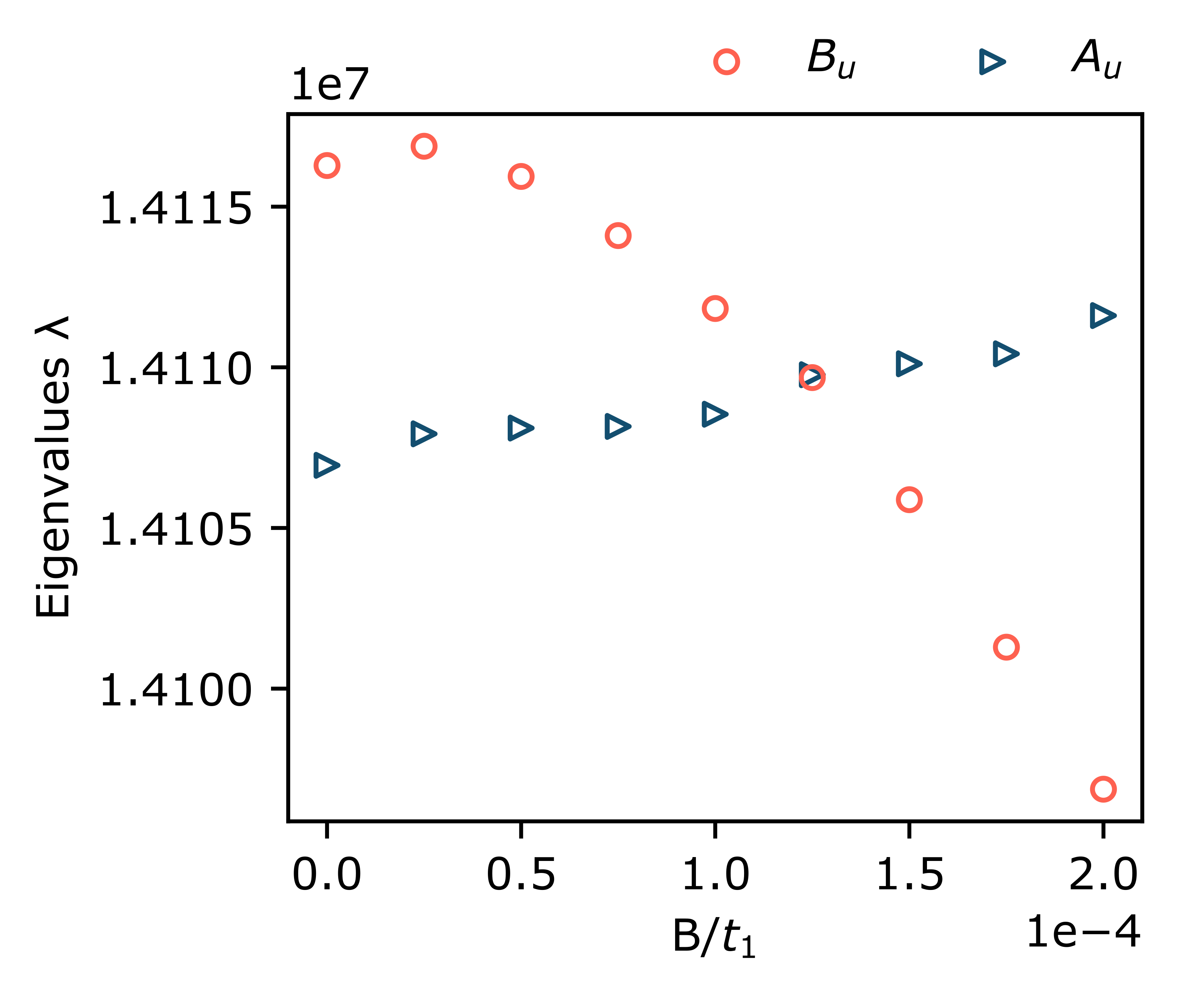
Figure 1: The two largest eigenvalues of the pair field susceptibility matrix $\chi$ as a function of applied magnetic field strength $B$, for a field aligned along the crystalline $b$-axis. This is found at a temperature $T=10^{-4}t_{1}$ and with approximately $6\times 10^{4}$ points on the Fermi surface. The dominant basis functions of type $B_{u}$ are $\tau_{0}\otimes(k_{x}\sigma_{y})(i\sigma_{y})$ and $\tau_{x}\otimes(k_{x}\sigma_{y})(i\sigma_{y})$, while the dominant basis functions of type $A_{u}$ are $\tau_{0}\otimes(k_{x}\sigma_{x})(i\sigma_{y})$ and $\tau_{x}\otimes(k_{x}\sigma_{x})(i\sigma_{y})$. At around $B=1.25\times 10^{-4}t_{1}$, there is a crossing between the largest eigenvalues, indicating a transition between pairing states.

Generically, if $D_{i}$ and $D_{j}$ belong to the same irreducible representation, $\chi_{ij}$ can be nonzero. Thus, the correct susceptibilities to compare are not those between the different basis functions but instead those between different eigenstates of $\chi$, which are mixtures of basis functions in the same irreducible representation. The eigenvalues of $\chi$ are still a proxy for the logarithm of the superconducting transition temperatures $T_{c}$, and the true superconducting order has the form of the eigenvector corresponding to the largest eigenvalue.

Fig. 1 shows the evolution of the largest eigenvalues of $\chi$ (Eq. 6) as a function of the applied magnetic field strength $B$. The eigenvalues are labeled by the symmetry classifications that their corresponding eigenvectors belong to. At low fields, states in the $B_{u}$ classification are favored, and spin-triplet states with $\vec{d}\parallel\hat{y}$ ($\tau_{x}\otimes k_{x}\sigma_{y}(i\sigma_{y})$ and $\tau_{0}\otimes k_{x}\sigma_{y}(i\sigma_{y})$) dominate. At a critical field strength of $B_{c}\sim 10^{-4}t_{1}$, there is a crossing of the largest eigenvalues, signalling a transition from $B_{u}$ to $A_{u}$. The dominant basis functions at high field are spin-triplet with $\vec{d}\parallel\hat{x}$ ($\tau_{x}\otimes k_{x}\sigma_{x}(i\sigma_{y})$ and $\tau_{0}\otimes k_{x}\sigma_{x}(i\sigma_{y})$).

This level crossing may be understood as a result of the competition between the magnetic field and spin-orbit coupling. At $B=0$, the spin-orbit coupling largely determines the pairing state to be in $B_{u}$, with a primary spin component in the $ac$ plane. Since this is energetically unfavorable in the presence of a magnetic field along the crystalline $b$ axis, increasing the magnetic field strength ultimately overwhelms the spin-orbit coupling and drives a transition to a $A_{u}$.

While the qualitative picture offered here is consistent with the experimental observations, we find that the relative splitting between eigenvalues (effective differences in $T_{c}$) between the two phases is very small. This may be an indication that the competition between spin-orbit coupling and the magnetic field is insufficient to fully explain the transition. In the next section, we consider the effects of ferromagnetic pairing interactions and assess the robustness of the results described above.

III.2 Self-consistent mean-field approach

Our analysis of the normal state instabilities suggests that, even without considering any specific pairing interactions, there is a tendency towards a transition between superconducting states with distinct pairing symmetries due to competition between spin-orbit coupling and applied magnetic field. We now account for interactions and determine the pairing states favored by a potential, rather than the kinetic, energy; we identify the nature (first- or second-order) of the transition between pairing symmetries and assess the effect of interactions on the value of the critical field $B_{c}$.

We consider an on-site, opposite-sublattice ferromagnetic interaction

$$H_{I}=-\left(\sum_{i}J_{x}S_{i,1}^{x}S_{i,2}^{x}+J_{y}S_{i,1}^{y}S_{i,2}^{y}+J_{z}S_{i,1}^{z}S_{i,2}^{z}\right),$$ (7)

where $i$ is a site index and $1,2$ are sublattice indices. While there are a plethora of other conceivable local interactions, we choose interactions of this particular form, as suggested by DFT calculationsXu et al. (2019) and supported by neutron scattering experiments Knafo et al. (2021). Note that the results of Ref. Knafo et al., 2021 suggest nearest neighbor antiferromagnetic interactions along the $y$ axis (favoring singlet pairing) and nearest-neighbor ferromagnetic interactions along the $x$ axis (favoring the states identified in Sec. III.1) in addition to the on-site ferromagnetic interactions we have chosen here. However, recent work incorporating this more general form of the interaction and a different normal-state HamiltonianChen et al. (2021) identifies the same zero-field state as we do, indicating that the results reported here are likely robust to these additional interactions.

To find the gap function $\Delta(k)$ in the presence of these interactions, we take a standard mean-field approach, decoupling the four-fermion interaction and defining the gap function in terms of the interaction. In the spin-orbit Nambu basis, the Bogoliubov deGennes (BdG) Hamiltonian takes the form

$$H_{BdG}=\begin{pmatrix}h(k)&\Delta(k)\\ \Delta^{\dagger}(k)&-h(-k)^{T}\end{pmatrix},$$ (8)

where $h(k)$ and $\Delta(k)$ are $4\times 4$ matrices, and has eigenvectors and eigenvalues satisfying

$$H_{BdG}\begin{pmatrix}\{u^{n}_{k\mu}\}\\ \{v^{n}_{-k\mu}\}\end{pmatrix}=E_{kn}\begin{pmatrix}\{u^{n}_{k\mu}\}\\ \{v^{n}_{-k\mu}\}\end{pmatrix}.$$ (9)

The mean-field self-consistency condition for $\Delta(k)$ is then

$$\Delta_{\mu\nu}(\vec{k}) =\sum_{\vec{k}^{\prime}}\sum_{\mu^{\prime}\nu^{\prime}}V_{\mu\nu\mu^{\prime}\nu^{\prime}}(\vec{k},\vec{k}^{\prime})$$

$$\times\sum_{n}\left[(u_{\vec{k^{\prime}\mu_{3}}})^{n}(v^{*}_{-\vec{k^{\prime}\mu_{4}}})^{n}\tanh\left(\frac{E_{\vec{k}^{\prime}n}}{2k_{B}T}\right)\right],$$ (10)

where $V_{\mu\nu\mu^{\prime}\nu^{\prime}}$ is the pairing interaction generated from Eq. 7 (see Sec. VII.2), the sum over $\vec{k}^{\prime}$ is over the Fermi surface, $\mu^{\prime}$ and $\nu^{\prime}$ are generalized spin-orbit indices, and $E_{kn}$, $u_{k\mu}^{n}$, and $v_{-k\mu}^{n}$ are defined by Eq. 9. In contrast to our approach in Sec. III.1, we do not assume a particular parity of the gap function. Instead, the solutions $\Delta(k)$ to Eq. 10 are generically admixtures of the basis functions in the orthorhombic symmetry group which are allowed by symmetry ($I$, $M_{i}$) to mix. Thus, the following results reveal which states are favored by the pairing interactions of Eq. 7, under the symmetry constraints provided by the normal-state Hamiltonian (Eq. 5).

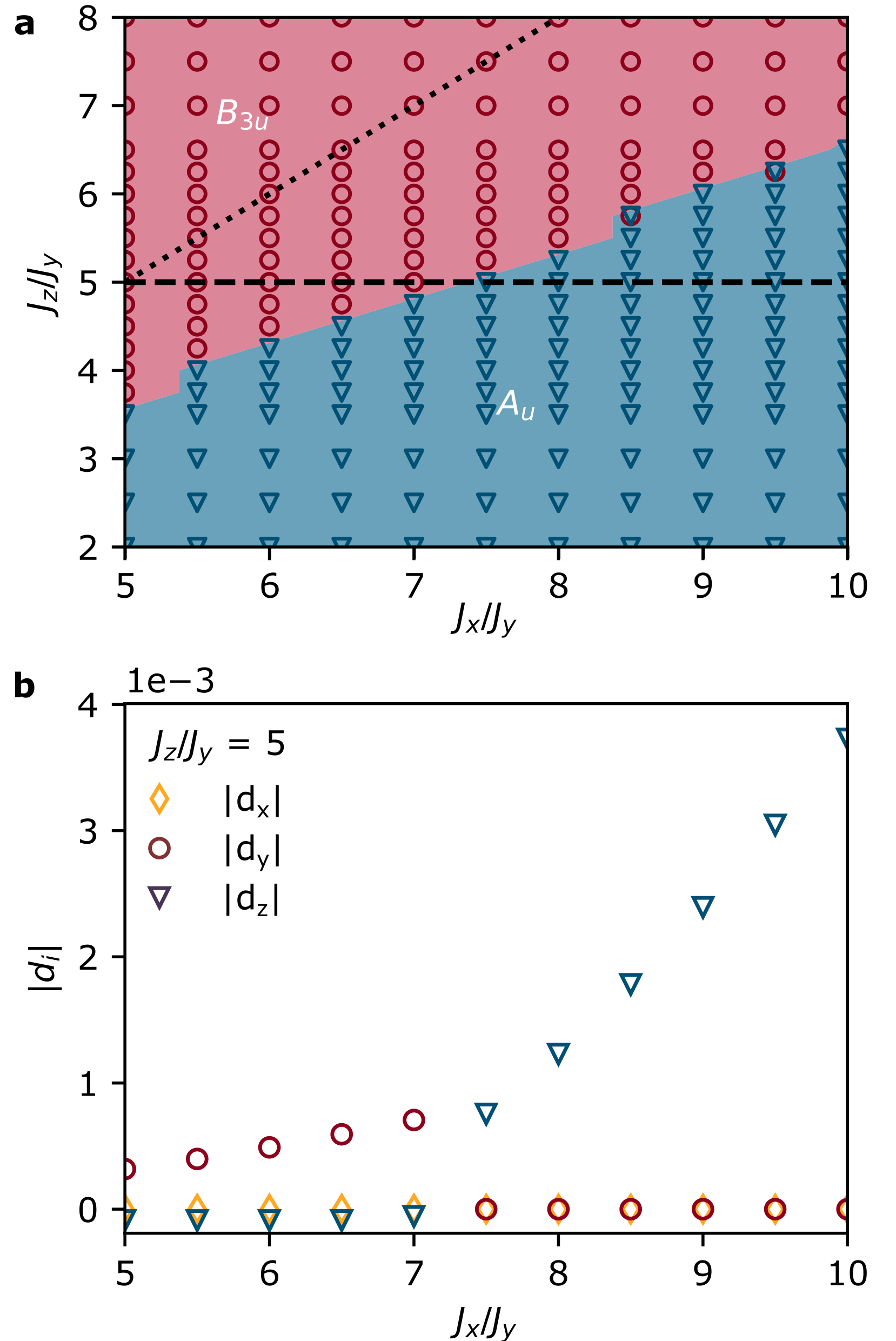
Figure 2: (a) The zero-field, zero-temperature ($B=0$, $T=0$) phase diagram in interaction parameter space obtained from solving the self-consistent gap equation numerically for $J_{y}=10^{-3}t_{1}$. Solutions are of the form $\Delta=\tau_{y}\otimes(\vec{d}\cdot\vec{\sigma})(i\sigma_{y})$ in the spin-orbit basis, with $\vec{d}=\vec{d}(J_{x},J_{y},J_{z})$. The dotted line denotes the separation between realistic ($J_{x}>J_{z}>J_{y}$) and unrealistic parameters, while the dashed line indicates the value of $J_{z}$ for the line cut plotted in Panel (b). (b) A representative line-cut in the space of parameters, showing a first-order transition between $B_{3u}$ and $A_{u}$ as a function of $J_{x}/J_{y}$. Shown are the magnitudes of $d_{i}$ ($i=x,y,z$) at $J_{z}/J_{y}=5$, which exhibit discontinuous jumps indicating a first-order transition between pairing states.

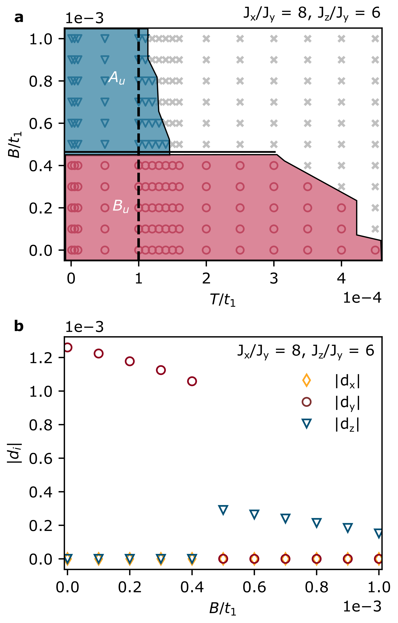
Figure 3: Solutions to the gap equation with interaction parameters $J_{x}/J_{y}=8$, $J_{y}=10^{-3}t_{1}$, $J_{z}/J_{y}=6$. (a) The phase diagram in temperature $T$ and magnetic field strength $B$ for a $\vec{B}=B\hat{y}$, as found by solving the gap equation (Eq. 10). In the red region, the superconducting gap function has the form $\tau_{y}\otimes d_{y}\sigma_{y}(i\sigma_{y})$, while in the blue region, the gap function has the form $\tau_{y}\otimes d_{z}\sigma_{z}(i\sigma_{y})$. The unshaded region indicates the region in which the gap function vanishes ($d_{x},d_{y},d_{z}<\epsilon$, for $\epsilon$ the error tolerance $\epsilon=10^{-5}t_{1}$), such that the system is in the normal state. The temperature-induced transitions are second-order (single line) while the field-induced transitions are first-order (double line). A dashed line at $T=10^{-4}t_{1}$ indicates the line cut examined in Panel (b). (b) Gap magnitudes $|d_{i}|$ ($i=x,y,z$) as a function of applied magnetic field strength $B$, for a field aligned along the crystalline $b$-axis at temperature $T=10^{-4}t_{1}$. At a field strength of approximately $B/t_{1}\sim 5\times 10^{-4}$, there is a first-order transition from the $B_{u}$ pairing state at low fields to the $A_{u}$ pairing state at high fields.

We solve Eq. 10 by iteration, starting with a random initial matrix $\Delta_{0}(\vec{k})$. We consider the solution to be converged after $n$ iterations when $\Delta_{n}$ and $\Delta_{n-1}$ satisfy the convergence condition $|\Delta_{n}(\vec{k})-\Delta_{n-1}(\vec{k})|<10^{-8}t_{1}\approx 1\text{ neV}$. Details of the this procedure are in Sec. VII.2.

While we allow for both even and odd parity solutions of Eq. 10, we have found that all non-trivial solutions have odd parity and take the form $\Delta=\tau_{y}\otimes(\vec{d}\cdot\vec{\sigma})(i\sigma_{y})$, where $\vec{d}$ is momentum-independent. For the remainder of this section, we will refer to the gap function by the orientation of $\vec{d}$, always implicitly assuming the form $\Delta=\tau_{y}\otimes(\vec{d}\cdot\vec{\sigma})(i\sigma_{y})$. We also absorb the gap magnitude into $\vec{d}$, such that $|\Delta|^{2}=|\vec{d}|^{2}$. In the same spirit as Ref. Chen et al., 2021, we will allow for anisotropy in the interactions. We first consider how $J_{x}$, $J_{y}$, and $J_{z}$ determine the pairing symmetries at zero-field ($B=0$) and identify realistic values for the exchange energies.

Fig. 2a is the phase diagram in the space of interaction parameters $J_{x}/J_{y}$ and $J_{z}/J_{y}$, for $B=0$, $T=0$, and $J_{y}=10^{-3}t_{1}$. At $B=0$, $\vec{d}\parallel\hat{x}$, $\vec{d}\parallel\hat{y}$, and $\vec{d}\parallel\hat{z}$ belong to distinct symmetry classifications (Table 1). The nature of the transitions between the pairing states as a function of the interactions $J_{x}$ and $J_{z}$ can be determined by analyzing the gap magnitudes. Fig. 2b shows the magnitudes of $d_{i}$ as a function of $J_{x}/J_{y}$ for a fixed $J_{z}/J_{y}=5$. This reveals a first-order transition between $B_{3u}$ and $A_{u}$ in the interaction parameter space at $B=0$.

The actual interactions present in UTe₂ are modeled well only by a region of the interaction space shown in Fig. 2a. Since the zero-field state is experimentally known to be suppressed by a $b$-axis magnetic field, we identify the $B_{3u}$ state ($\vec{d}\parallel\hat{y}$) as a good candidate for the low-field state, as it is a triplet state with spin in the $ac$ plane. As shown in Fig. 2a, the $B_{3u}$ state is favored for interactions $J_{x},J_{z}>J_{y}$. The parameter range in which we find a $B_{3u}$ state is consistent with expectations from the magnetic properties of the normal state. Since the $a$ axis is the easy magnetic axis, and the $b$ axis is the hard magnetic axis Ran et al. (2019), the physical interaction parameters are likely $J_{x}>J_{z}>J_{y}$. The separation between the realistic and unrealistic interaction parameter regimes is shown in Fig. 2a as a dotted line.

So far, we have solved the self-consistency equation (Eq. 10) for the gap function at $B=0$ and $T=0$, for a variety of interactions. We now consider the behavior of the gap at finite temperature and magnetic field and construct a phase diagram in the space of temperature $T$ and applied field $B$ (along the $\hat{y}$ axis), shown in Fig. 3a. Specifically, we investigate the nature of the transition between the $B_{u}$ low-field state and the $A_{u}$ high-field state as a function of applied field strength, as shown in Fig. 3b.

We choose a representative set of parameters corresponding to a gap in the phase $B_{3u}$ ($\vec{d}\parallel\hat{y}$) at $B=0$ and $T=0$: $J_{x}/J_{y}=8$, $J_{z}/J_{y}=6$, and $J_{y}=10^{-3}t_{1}$. We then solve the self-consistent gap equation (Eq. 10) with $B>0$ and $T>0$. As shown in Fig. 3a, at a finite field $B>0$, there is a first-order transition between the pairing states with $\vec{d}\parallel\hat{y}$ and $\vec{d}\parallel\hat{z}$, while finite temperature transitions between the superconducting states and the normal state remain second-order. In principle, the high-field $A_{u}$ state could be an mixture of the $\vec{d}\parallel\hat{x}$ and $\vec{d}\parallel{z}$ states (see Table 2), but we find that any $\vec{d}\parallel\hat{x}$ is suppressed by the large value of $J_{x}$.

Fig. 3b shows the evolution of $\vec{d}$ as a function of the applied magnetic field strength $B/t_{1}$. Upon increasing $B$, the $B_{u}$ state is suppressed, and we observe a first-order transition to $A_{u}$ pairing symmetry at around $B/t_{1}=5\times 10^{-4}$. The transition is between the same symmetry classifications as those identified in Sec. III.1, but the transition occurs at an enhanced critical field $B_{c}$, which may be attributed to the cooperation between spin-orbit coupling and interactions to stabilize of the low-field state.

IV Properties of the Low- and High- Field Phases

IV.1 Sensitivity to angle

The low- and high-field superconducting phases in UTe₂ are distinguished by their sensitivity (or lack thereof) to the angle of the applied magnetic field with respect to the crystalline $b$ axis; the high-field phase is sensitive to the angle of the field, whereas the low-field phase is not. We now show that our results are consistent with this observation through a qualitative argument and by providing numerical evidence in support of this claim.

From both the analysis of the superconducting susceptibility and of the mean-field solution in the presence of ferromagnetic interactions, we find that the low-field phase is a triplet state with primarily $\vec{d}\parallel\hat{y}$, whereas the high-field phase has primarily $\vec{d}\parallel\hat{x}$ or $\vec{d}\parallel\hat{z}$.

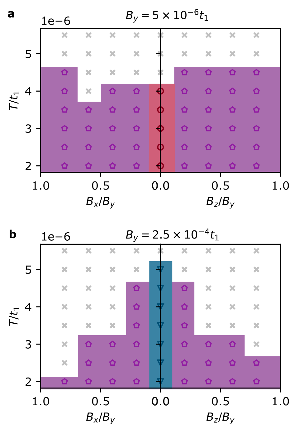
Figure 4: Phase diagrams in temperature $T$ and magnetic fields $B_{x}$ or $B_{z}$, for solutions of the gap equation with interaction parameters $(J_{x},J_{y},J_{z})=(2.8\times 10^{-3}t_{1},1.5\times 10^{-3}t_{1},2.6\times 10^{-3}t_{1})$ for (a) $B_{y}=5\times 10^{-6}t_{1}$ and (b) $B_{y}=2.5\times 10^{-4}t_{1}$. At $B_{x}=B_{z}=0$, the solution at (a) $B_{y}=5\times 10^{-6}t_{1}$ is $\tau_{y}\otimes(d_{z}\sigma_{y})(i\sigma_{y})$ (red shaded region, circles), and the solution at (b) $B_{y}=2.5\times 10^{-4}t_{1}$ is $\tau_{y}\otimes(d_{z}\sigma_{z})(i\sigma_{y})$ (blue shaded region, triangles). In the presence of a field misaligned with the crystal axes, all mirror symmetries are broken, and there is only one irreducible representation (purple shaded region, pentagons). The unshaded region indicates the region in which the gap function vanishes ($d_{x},d_{y},d_{z}<\epsilon$, for $\epsilon$ the error tolerance $\epsilon=1\times 10^{-6}t_{1}$), such that the system is no longer superconducting.

Since the spin in a triplet state is proportional to $\vec{d}\times\vec{d}^{*}$, a state with $\vec{d}\parallel\hat{y}$ (spin in the $xz$ plane) will be suppressed in the presence of a large magnetic field along the $\hat{y}$ direction. However, such a state should be relatively insensitive to a field in the $\hat{x}$ or $\hat{z}$ directions. This is consistent with the experimental results in the low-field phase. In contrast, the high-field $A_{u}$ phase with $\vec{d}=d_{x}\hat{x}+d_{z}\hat{z}$ is stable to large fields along $\hat{y}$ but is suppressed by fields along $\hat{x}$ or $\hat{z}$. More concretely, the suppression of a given pairing state by a time-reversal symmetry breaking perturbation may be quantified by the field fitness function Ramires and Sigrist (2016); Ramires et al. (2018); Cavanagh et al. (2022). For example, spin-orbit coupling determines how severely the specific high-field solution $\tau_{y}\otimes(d_{z}\sigma_{z})(i\sigma_{y})$ found in Sec. III.2 is suppressed by tilting of the field in the $a$ and $c$ directions (see Sec. VII.3).

We also explicitly demonstrate the responses of states identified in Sec. III.2 to magnetic fields off of the $b$ axis. Specifically, we again solve the gap equation (Eq. 10) at various temperatures $T$ and with interactions $(J_{x},J_{y},J_{z})=(2.8\times 10^{-3}t_{1},1.5\times 10^{-3}t_{1},2.6\times 10^{-3}t_{1})$. We consider two fixed values of $B_{y}$, corresponding to the low-field state at $\vec{B}=(0,5\times 10^{-6}t_{1},0)$ and the high-field state at $\vec{B}=(0,2.5\times 10^{-4}t_{1},0)$ and introduce finite $B_{x}$ and $B_{z}$. As shown in Fig. 4, the critical temperature of the low-field state does not change significantly upon the introduction of $B_{x}$ or $B_{z}$. In contrast, the critical temperature of the high-field state decreases with increasing $B_{x}$ or $B_{z}$. Qualitatively, this matches the experimental observationsRosuel et al. (2022); Kinjo et al. (2022).

IV.2 Nodal structure

We now consider the nodal structure of the gap functions found in the self-consistent calculation. Calorimetric measurementsKittaka et al. (2020); Metz et al. (2019); Ran et al. (2019); Bae et al. (2021), magnetic penetration depth measurements Ishihara et al. (2022), and NMR $1/T_{1}$ relaxation rate measurements Nakamine et al. (2019) in UTe₂ at zero-field show evidence of point nodes in the superconducting gap function, but there is no global consensus on the locations of these nodes. From the self-consistent solution to Eq. 10 in zero field ($B=0$), we find that the candidate zero-field ($B_{3u}$) phase has point nodes along the $a$ axis.

In a one-band system, the nodal structure of a gap can be deduced from its symmetry classification. This is because the momentum dependence of the basis functions dictates the nature of the nodes (none, point, or line). However, in a multiband system, the nodal structure cannot be straightforwardly related to the symmetry classification of the gap, as the basis functions gain nontrivial structure in the band basis Agterberg et al. (2017a, b); Zhou et al. (2008).

We thus identify the nodal structure of the solution to Eq. 10 by projecting $\Delta$ into the band basis. To simplify our calculation, we consider the projection only at $k_{z}=0$ ($f_{z}=f_{u}=0$) (see Sec. VII.4). For a given pairing state, the stable nodes are those which are not suppressed by adding an arbitrary mixture of other pairing states within the same symmetry classification. The projection at $k_{z}=0$ yields that the candidate zero-field ($B_{3u}$) phase has stable point nodes along the $a$ axis. These results are consistent with transport measurements Metz et al. (2019) which identify point nodes in the $ab$ plane and field-angle-resolved measurements of the specific heat Kittaka et al. (2020) which identify point nodes along the $a$ axis for the zero-field superconducting state.

V Discussion

In this work, we have determined the pairing symmetries of the low- and high-field phases of UTe₂ within mean field theory for a minimal Hamiltonian. We find that the field-induced transition between pairing symmetries in UTe₂ is a transition from states of the $B_{u}$ classification at low fields to states of the $A_{u}$ classification at high fields. These pairing states are consistent with the experimental signatures within each phase, namely the suppression of the high-field phase upon tilting the magnetic field away from the $b$ axis and the lack thereof in the low-field phase. Furthermore, our predictions of the nodal structure of the gap at zero-field are consistent with the results of thermal transport measurements.

However, the $T-B$ phase diagram found in our calculations (Fig. 3a) does not reflect the phenomenon of reentrant superconductivity. This suggests that fluctuations, which are neglected in our mean-field approach, may be responsible for an increase of $T_{c}$ with increasing $B$ in the high-field phase. The details of reentrant superconductivity and other the phenomena in UTe₂ are also undoubtedly influenced by factors such as disorderRosa et al. (2022), vortex formationIguchi et al. (2022), and orbital-field coupling, which we have also neglected. Even so, the minimal model used here, which includes only the most essential structural elements of UTe₂, captures the field-driven transition between different pairing symmetries and qualitative signatures of these high- and low-field phases at low temperatures. This suggests that the orthorhombic crystal symmetry and sublattice structure of UTe₂ play the largest roles in determining its superconducting states.

While our approach using itinerant electrons successfully determines the nature of superconductivity in UTe₂, the underlying mechanisms behind superconductivity remain unexplained. Specifically, we assume here a particular form for the local ferromagnetic interaction (Eq. 7) and a specific hierarchy of the anisotropic spin-orbit couplings. A derivation of the interaction and SOC are beyond the scope of this work, but we acknowledge that symmetry principles can justify the general form of the model and the anisotropic nature of the interactions and SOC but cannot fully explain the origins of these terms. Below, we conjecture how a complementary perspective may supply a satisfactory conceptual understanding.

UTe₂ is found to have signatures of a strong-coupling superconductor, and agreement between DFT and experiments depends sensitively on the Hubbard interaction parameterAoki et al. (2022), suggesting that correlation effects in UTe₂ are essential. Thus, the more fundamental questions about the origins of interactions and mechanisms responsible for superconductivity may be better answered from a perspective of local, microscopic physics complementary to the one presented here. More generally, a complete description of the phenomena in UTe₂ and related heavy-fermion superconductors likely requires a combination of both the local and itinerant perspectives.

VI Acknowledgements

We thank S. Brown, T. Hazra for helpful discussions. JJY was supported by the National Science Foundation Graduate Research Fellowship under Grant No. DGE-1656518. SR was supported in part by the US Department of Energy, Office of Basic Energy Sciences, Division of Materials Sciences and Engineering, under contract number DE-AC02-76SF00515. DFA and YY were supported by by the US Department of Energy, Office of Basic Energy Sciences, Division of Materials Sciences and Engineering under Award DE-SC0021971.

VII Appendix

VII.1 Parameters of the tight-binding model

The constants in Eq. 2 and Eq. 3 used in this work are listed here. For the calculation of the pair-field susceptibility and its eigenvalues and eigenstates (Sec. III.1), we use $(t_{1},\mu,t_{2},m_{0},t_{3},t_{z},t_{x},t_{y},t_{u})=(-1,1.446,0.76,-0.695,0.83,-0.83,0.785,0.224,0.112)$. For the solution of the self-consistent gap equation (Sec. III.2), we use $(t_{1},\mu,t_{2},m_{0},t_{3},t_{z},t_{x},t_{y},t_{u})=(-1,1.446,0.76,-0.695,0.83,-0.83,0.448,0.224,0.112)$. In Sec. IV.1, we use $(t_{1},\mu,t_{2},m_{0},t_{3},t_{z},t_{x},t_{y},t_{u})=(-1,1.446,0.76,-0.695,0.83,-0.83,0.15,0.12,0.11)$.

VII.2 Solving the self-consistent gap equation with ferromagnetic interactions

Generically, a two-body interaction in real space takes the form $H_{I}=\sum_{i,j}\sum_{\mu,\nu,\mu^{\prime},\nu^{\prime}}U_{i}^{\mu\nu\mu^{\prime}\nu^{\prime}}c^{\dagger}_{i,\mu}c_{i,\mu^{\prime}}c^{\dagger}_{j,\nu}c_{j,\nu^{\prime}}$. Here, $i$ and $j$ are site labels, while $\mu(^{\prime}),\nu(^{\prime})$ are generalized spin-orbit indices. Via a Fourier transform, one can always express this interaction in BCS form as

$$H_{I}=\sum_{k,k^{\prime}}V_{\mu_{1},\mu_{2},\mu_{3},\mu_{4}}(\vec{k},\vec{k}^{\prime})c_{k,\mu_{1}}^{\dagger}c_{-k,\mu_{2}}^{\dagger}c_{-k^{\prime},\mu_{3}}c_{k^{\prime},\mu_{4}},$$ (11)

where $V$ is the effective BCS pairing interaction entering Eq. 10 and repeated indices are summed over.

For the local ferromagnetic interaction described in Eq. 7,

$$V_{\mu_{1},\mu_{2},\mu_{3},\mu_{4}}(\vec{k},\vec{k}^{\prime})c_{k,\mu_{1}}^{\dagger}c_{-k,\mu_{2}}^{\dagger}c_{-k^{\prime},\mu_{3}}c_{k^{\prime},\mu_{4}} =\sum_{a=x,y,z}J_{a}\sigma_{a}^{s^{\prime}s}\sigma_{a}^{p^{\prime}p}c_{k,\tau=1,s^{\prime}}^{\dagger}c_{-k,\tau=2,p^{\prime}}^{\dagger}c_{-k^{\prime},\tau=2,s}c_{k^{\prime},\tau=1,p}.$$ (12)

for $\sigma_{a}$ Pauli matrices on the spins and $\tau$ indexing the sublattices.

Then, the matrix $V$ is written:

$$V_{\mu_{1},\mu_{2},\mu_{3},\mu_{4}}(\vec{k},\vec{k}^{\prime})=\epsilon^{\mu_{1}\mu_{2}}\epsilon^{\mu_{3}\mu_{4}}\sum_{a=x,y,z}\frac{J_{a}}{2}\left[\left(P^{\tau}_{1}\sigma_{a}\right)^{\mu_{1}\mu_{4}}\left(P^{\tau}_{2}\sigma_{a}\right)^{\mu_{2}\mu_{3}}+\left(P^{\tau}_{2}\sigma_{a}\right)^{\mu_{1}\mu_{4}}\left(P^{\tau}_{1}\sigma_{a}\right)^{\mu_{2}\mu_{3}}\right]$$ (13)

We use iteration to solve the self-consistent gap equation Eq. 10 with the interactions described by Eq. 13.

VII.3 Field-fitness functions for the solutions of the gap equation

While the numerical solutions to the gap equation show how the gap magnitudes of different pairing states evolve under a magnetic field, they do not offer insight as to what controls the suppression of a given pairing state by a given field. We quantify the pair-breaking effects of a magnetic field on the solutions of the self-consistent gap equation ($\tau_{y}\otimes\sigma_{y}(i\sigma_{y})$ at low fields and $\tau_{y}\otimes\sigma_{z}(i\sigma_{y})$ at high fields) by the field-fitness function as defined by Cavanagh et. al. Cavanagh et al. (2022). If the field-fitness function for a given pairing state and perturbation vanishes ($F_{k}=0$), then the perturbation does not have any depairing effects; on the other hand, $F_{k}=1$ indicates maximal pair-breaking.

To understand the suppression of the high-field phase, we find the field-fitness functions for $\tau_{y}\otimes\sigma_{z}(i\sigma_{y})$ in a magnetic field in the $\hat{x}$ or $\hat{z}$ directions. The result is:

$$F_{k}(B\parallel\hat{x})^{d\parallel z} \propto\frac{f_{x}^{2}f_{Ag}^{2}}{(f_{x}^{2}+f_{y}^{2}+f_{z}^{2})(f_{z}^{2}+f_{Ag}^{2}+f_{y}^{2})}$$ (14)

$$F_{k}(B\parallel\hat{z})^{d\parallel z} \propto\frac{f_{z}^{2}(f_{x}^{2}+f_{y}^{2}+f_{z}^{2}+f_{Au}^{2}+f_{Ag}^{2})}{(f_{x}^{2}+f_{y}^{2}+f_{z}^{2})(f_{z}^{2}+f_{Au}^{2}+f_{Ag}^{2})}$$ (15)

Generically, these will be nonzero over the Fermi surface, thus resulting in suppression of the high-field phase.

We compare these to the field-fitness functions of the low-field phase:

$$F_{k}(B\parallel\hat{x})^{d\parallel y} \propto\frac{f_{Au}^{2}f_{Ag}^{2}}{(f_{z}^{2}+f_{y}^{2}+f_{Au}^{2})(f_{z}^{2}+f_{Ag}^{2}+f_{y}^{2})}$$ (16)

$$F_{k}(B\parallel\hat{z})^{d\parallel y} \propto\frac{f_{y}^{2}f_{Ag}^{2}}{(f_{z}^{2}+f_{y}^{2}+f_{Au}^{2})(f_{z}^{2}+f_{Ag}^{2}+f_{Au}^{2})}$$ (17)

The kinetic energy scale is taken to be larger than the spin-orbit coupling energy scale: $f_{z}^{2},f_{Ag}^{2}>f_{y}^{2},f_{x}^{2},f_{Au}^{2}$.

Since the x-direction is the shortest bond, we expect that $f_{x}>f_{Au}$. This leads to $F_{k}(B\parallel x)^{d\parallel z}>F_{k}(B\parallel x)^{d\parallel y}$.

Additionally, $F_{k}(B\parallel z)^{d\parallel z}>F_{k}(B\parallel z)^{d\parallel y}$ for a similar reason. In summary, we argue here that the low-field $B_{u}$ phase is less suppressed by fields in the $\hat{x}$ and $\hat{z}$ directions than the high-field $A_{u}$ phase; this agrees with experimental results and the claims in Sec. IV, and it provides some intuition for the terms responsible for pairing suppression.

VII.4 Gap functions in the band basis

In the band basis, the basis functions may be projected onto a single band. The momentum dependence of the gap in the band basis determines the nodal structure. Since basis functions of a given symmetry are able to mix, we identify nodes of a given symmetry as those which survive under arbitrary mixing of the basis functions.

Tables 3 and 4 list the momentum dependence of each basis function in Table 1 found using simplified Hamiltonian at $k_{z}=0$. From the momentum dependence of the basis functions in each irreducible representation, we find that arbitrary mixtures of functions in the $B_{1u}$ classification have point nodes where $k_{x}=0,\pm\pi$ and $k_{y}=0,\pm\pi$; mixtures of $B_{2u}$ have point nodes where $k_{x}=0,\pm\pi$ and $k_{z}=0,\pm\pi$; and mixtures of $B_{3u}$ have point nodes where $k_{y}=0,\pm\pi$ and $k_{z}=0,\pm\pi$. Mixtures of the $A_{u}$ basis functions have no nodes generically.

$\Delta$ (SO basis)	$D_{2h}$ Classification	Momentum dependence
$\tau_{0}k_{y}\sigma_{x}(i\sigma_{y})$	$B_{1u}$	$\sin k_{y}\left(\frac{f_{y}}{\sqrt{f_{x}^{2}+f_{y}^{2}}}\hat{z}+\frac{f_{Ag}^{2}f_{x}}{\sqrt{f_{x}^{2}+f_{y}^{2}}(f_{Ag}^{2}+f_{x}^{2}+f_{y}^{2}+\sqrt{(f_{x}^{2}+f_{y}^{2})(f_{Ag}^{2}+f_{x}^{2}+f_{y}^{2})}}\hat{y}\right)$
$\tau_{0}k_{x}\sigma_{y}(i\sigma_{y})$	$B_{1u}$	$\sin k_{x}\left(\frac{f_{x}}{\sqrt{f_{x}^{2}+f_{y}^{2}}}\hat{z}+\frac{f_{Ag}^{2}f_{y}}{\sqrt{f_{x}^{2}+f_{y}^{2}}(f_{Ag}^{2}+f_{x}^{2}+f_{y}^{2}+\sqrt{(f_{x}^{2}+f_{y}^{2})(f_{Ag}^{2}+f_{x}^{2}+f_{y}^{2})})}\hat{x}\right)$
$\tau_{x}k_{y}\sigma_{x}(i\sigma_{y})$	$B_{1u}$	$\sin k_{y}\left(\frac{f_{x}}{\sqrt{f_{x}^{2}+f_{y}^{2}}}\hat{y}+\frac{f_{Ag}f_{y}}{\sqrt{f_{x}^{2}+f_{y}^{2}}(\sqrt{f_{Ag}^{2}+f_{x}^{2}+f_{y}^{2}}+\sqrt{f_{x}^{2}+f_{y}^{2}})}\hat{z}\right)+\sin k_{y}\frac{f_{Ag}f_{y}}{f_{Ag}^{2}+f_{x}^{2}+f_{y}^{2}+\sqrt{(f_{x}^{2}+f_{y}^{2})(f_{Ag}^{2}+f_{x}^{2}+f_{y}^{2})}}$
$\tau_{x}k_{x}\sigma_{y}(i\sigma_{y})$	$B_{1u}$	$\sin k_{x}\left(-\frac{f_{y}}{\sqrt{f_{x}^{2}+f_{y}^{2}}}\hat{y}+\frac{f_{Ag}f_{x}}{\sqrt{f_{x}^{2}+f_{y}^{2}}(\sqrt{f_{Ag}^{2}+f_{x}^{2}+f_{y}^{2}}+\sqrt{f_{x}^{2}+f_{y}^{2}})}\hat{z}\right)+\sin k_{x}\frac{f_{Ag}f_{x}}{f_{Ag}^{2}+f_{x}^{2}+f_{y}^{2}+\sqrt{(f_{x}^{2}+f_{y}^{2})(f_{Ag}^{2}+f_{x}^{2}+f_{y}^{2})}}$
$\tau_{z}(i\sigma_{y})$	$B_{1u}$	$\frac{f_{x}^{2}+f_{y}^{2}+\sqrt{(f_{x}^{2}+f_{y}^{2})(f_{Ag}^{2}+f_{x}^{2}+f_{y}^{2})}}{f_{Ag}^{2}+f_{x}^{2}+f_{y}^{2}+\sqrt{(f_{x}^{2}+f_{y}^{2})(f_{Ag}^{2}+f_{x}^{2}+f_{y}^{2})}}$
$\tau_{0}k_{z}\sigma_{y}(i\sigma_{y})$	$B_{3u}$	$\sin k_{z}\left(\frac{f_{x}}{\sqrt{f_{x}^{2}+f_{y}^{2}}}\hat{z}+\frac{f_{Ag}^{2}f_{y}}{\sqrt{f_{x}^{2}+f_{y}^{2}}(f_{Ag}^{2}+f_{x}^{2}+f_{y}^{2}+\sqrt{(f_{x}^{2}+f_{y}^{2})(f_{Ag}^{2}+f_{x}^{2}+f_{y}^{2})})}\hat{x}\right)$
$\tau_{0}k_{y}\sigma_{z}(i\sigma_{y})$	$B_{3u}$	$\sin k_{y}\frac{f_{Ag}}{\sqrt{f_{Ag}^{2}+f_{x}^{2}+f_{y}^{2}}}\hat{x}$
$\tau_{x}k_{z}\sigma_{y}(i\sigma_{y})$	$B_{3u}$	$\sin k_{z}\left(-\frac{f_{y}}{\sqrt{f_{x}^{2}+f_{y}^{2}}}\hat{y}+\frac{f_{Ag}f_{x}}{\sqrt{f_{x}^{2}+f_{y}^{2}}(\sqrt{f_{Ag}^{2}+f_{x}^{2}+f_{y}^{2}}+\sqrt{f_{x}^{2}+f_{y}^{2}})}\hat{z}\right)+\sin k_{z}\frac{f_{Ag}f_{x}}{f_{Ag}^{2}+f_{x}^{2}+f_{y}^{2}+\sqrt{(f_{x}^{2}+f_{y}^{2})(f_{Ag}^{2}+f_{x}^{2}+f_{y}^{2})}}$
$\tau_{x}k_{y}\sigma_{z}(i\sigma_{y})$	$B_{3u}$	$\sin k_{y}\hat{x}$
$\tau_{y}\sigma_{y}(i\sigma_{y})$	$B_{3u}$	$\frac{f_{y}}{\sqrt{(f_{Ag}^{2}+f_{x}^{2}+f_{y}^{2})}}\hat{x}\sim\sin k_{y}\hat{x}$

Table 3: Momentum dependence of the low-field phase: $B_{u}$ (in-field) basis functions in the band basis.

$\Delta$ (SO basis)	$D_{2h}$ Classification	Momentum dependence
$\tau_{0}k_{x}\sigma_{x}(i\sigma_{y})$	$A_{u}$	$\sin k_{x}\left(\frac{f_{y}}{\sqrt{f_{x}^{2}+f_{y}^{2}}}\hat{z}+\frac{f_{Ag}^{2}f_{x}}{\sqrt{f_{x}^{2}+f_{y}^{2}}(f_{Ag}^{2}+f_{x}^{2}+f_{y}^{2}+\sqrt{(f_{x}^{2}+f_{y}^{2})(f_{Ag}^{2}+f_{x}^{2}+f_{y}^{2})}}\hat{y}\right)$
$\tau_{0}k_{y}\sigma_{y}(i\sigma_{y})$	$A_{u}$	$\sin k_{y}\left(\frac{f_{x}}{\sqrt{f_{x}^{2}+f_{y}^{2}}}\hat{z}+\frac{f_{Ag}^{2}f_{y}}{\sqrt{f_{x}^{2}+f_{y}^{2}}(f_{Ag}^{2}+f_{x}^{2}+f_{y}^{2}+\sqrt{(f_{x}^{2}+f_{y}^{2})(f_{Ag}^{2}+f_{x}^{2}+f_{y}^{2})})}\hat{x}\right)$
$\tau_{0}k_{z}\sigma_{z}(i\sigma_{y})$	$A_{u}$	$\sin k_{z}\frac{f_{Ag}}{\sqrt{f_{Ag}^{2}+f_{x}^{2}+f_{y}^{2}}}\hat{x}$
$\tau_{x}k_{x}\sigma_{x}(i\sigma_{y})$	$A_{u}$	$\sin k_{x}\left(\frac{f_{x}}{\sqrt{f_{x}^{2}+f_{y}^{2}}}\hat{y}+\frac{f_{Ag}f_{y}}{\sqrt{f_{x}^{2}+f_{y}^{2}}(\sqrt{f_{Ag}^{2}+f_{x}^{2}+f_{y}^{2}}+\sqrt{f_{x}^{2}+f_{y}^{2}})}\hat{z}\right)+\sin k_{x}\frac{f_{Ag}f_{y}}{f_{Ag}^{2}+f_{x}^{2}+f_{y}^{2}+\sqrt{(f_{x}^{2}+f_{y}^{2})(f_{Ag}^{2}+f_{x}^{2}+f_{y}^{2})}}$
$\tau_{x}k_{y}\sigma_{y}(i\sigma_{y})$	$A_{u}$	$\sin k_{y}\left(-\frac{f_{y}}{\sqrt{f_{x}^{2}+f_{y}^{2}}}\hat{y}+\frac{f_{Ag}f_{x}}{\sqrt{f_{x}^{2}+f_{y}^{2}}(\sqrt{f_{Ag}^{2}+f_{x}^{2}+f_{y}^{2}}+\sqrt{f_{x}^{2}+f_{y}^{2}})}\hat{z}\right)+\sin k_{y}\frac{f_{Ag}f_{x}}{f_{Ag}^{2}+f_{x}^{2}+f_{y}^{2}+\sqrt{(f_{x}^{2}+f_{y}^{2})(f_{Ag}^{2}+f_{x}^{2}+f_{y}^{2})}}$
$\tau_{x}k_{z}\sigma_{z}(i\sigma_{y})$	$A_{u}$	$\sin k_{z}\hat{x}$
$\tau_{y}\sigma_{z}(i\sigma_{y})$	$A_{u}$	$\frac{\sqrt{f_{x}^{2}+f_{y}^{2}}}{\sqrt{(f_{Ag}^{2}+f_{x}^{2}+f_{y}^{2})}}\hat{x}$
$\tau_{0}k_{z}\sigma_{x}(i\sigma_{y})$	$B_{2u}$	$\sin k_{z}\left(\frac{f_{y}}{\sqrt{f_{x}^{2}+f_{y}^{2}}}\hat{z}+\frac{f_{Ag}^{2}f_{x}}{\sqrt{f_{x}^{2}+f_{y}^{2}}(f_{Ag}^{2}+f_{x}^{2}+f_{y}^{2}+\sqrt{(f_{x}^{2}+f_{y}^{2})(f_{Ag}^{2}+f_{x}^{2}+f_{y}^{2})}}\hat{y}\right)$
$\tau_{0}k_{x}\sigma_{z}(i\sigma_{y})$	$B_{2u}$	$\sin k_{x}\frac{f_{Ag}}{\sqrt{f_{Ag}^{2}+f_{x}^{2}+f_{y}^{2}}}\hat{x}$
$\tau_{x}k_{z}\sigma_{x}(i\sigma_{y})$	$B_{2u}$	$\sin k_{z}\left(\frac{f_{x}}{\sqrt{f_{x}^{2}+f_{y}^{2}}}\hat{y}+\frac{f_{Ag}f_{y}}{\sqrt{f_{x}^{2}+f_{y}^{2}}(\sqrt{f_{Ag}^{2}+f_{x}^{2}+f_{y}^{2}}+\sqrt{f_{x}^{2}+f_{y}^{2}})}\hat{z}\right)+\sin k_{z}\frac{f_{Ag}f_{y}}{f_{Ag}^{2}+f_{x}^{2}+f_{y}^{2}+\sqrt{(f_{x}^{2}+f_{y}^{2})(f_{Ag}^{2}+f_{x}^{2}+f_{y}^{2})}}$
$\tau_{x}k_{x}\sigma_{z}(i\sigma_{y})$	$B_{2u}$	$\sin k_{x}\hat{x}$
$\tau_{y}\sigma_{x}(i\sigma_{y})$	$B_{2u}$	$\frac{f_{x}}{\sqrt{(f_{Ag}^{2}+f_{x}^{2}+f_{y}^{2})}}\hat{x}\sim\sin k_{x}\hat{x}$

Table 4: Momentum dependence of the high-field phase: $A_{u}$ (in-field) basis functions in the band basis

References

• Ran etΒ al. (2019) S.Β Ran, C.Β Eckberg, Q.-P. Ding, Y.Β Furukawa, T.Β Metz, S.Β R. Saha, I.-L. Liu, M.Β Zic, H.Β Kim, J.Β Paglione, etΒ al., Science 365, 684 (2019).
• Helm etΒ al. (2022) T.Β Helm, M.Β Kimata, K.Β Sudo, A.Β Miyata, J.Β Stirnat, T.Β FΓΆrster, J.Β Hornung, M.Β KΓΆnig, I.Β Sheikin, A.Β Pourret, etΒ al., Suppressed magnetic scattering sets conditions for the emergence of 40 T high-field superconductivity in UTe$_2$ (2022), eprint arXiv:2207.08261.
• Saxena etΒ al. (2000) S.Β S. Saxena, P.Β Agarwal, K.Β Ahilan, F.Β M. Grosche, R.Β K. Haselwimmer, M.Β J. Steiner, E.Β Pugh, I.Β R. Walker, S.Β R. Julian, P.Β Monthoux, etΒ al., Nature 406, 587 (2000), ISSN 1476-4687.
• Aoki etΒ al. (2001) D.Β Aoki, A.Β Huxley, E.Β Ressouche, D.Β Braithwaite, J.Β Flouquet, J.Β P. Brison, E.Β Lhotel, and C.Β Paulsen, Nature 413, 613 (2001), ISSN 0028-0836.
• Huy etΒ al. (2007) N.Β T. Huy, A.Β Gasparini, D.Β E. de Nijs, Y.Β Huang, J.Β C.Β P. Klaasse, T.Β Gortenmulder, A.Β de Visser, A.Β Hamann, T.Β GΓΆrlach, and H.Β v.Β LΓΆhneysen, Physical Review Letters 99, 067006 (2007).
• Aoki and Flouquet (2012) D.Β Aoki and J.Β Flouquet, Journal of the Physical Society of Japan 81, 011003 (2012), ISSN 0031-9015.
• Knebel etΒ al. (2019) G.Β Knebel, W.Β Knafo, A.Β Pourret, Q.Β Niu, M.Β ValiΕ‘ka, D.Β Braithwaite, G.Β Lapertot, M.Β Nardone, A.Β Zitouni, S.Β Mishra, etΒ al., Journal of the Physical Society of Japan 88, 063707 (2019), ISSN 0031-9015.
• Jiao etΒ al. (2020) L.Β Jiao, S.Β Howard, S.Β Ran, Z.Β Wang, J.Β O. Rodriguez, M.Β Sigrist, Z.Β Wang, N.Β P. Butch, and V.Β Madhavan, Nature 579, 523 (2020), ISSN 1476-4687.
• Hayes etΒ al. (2021) I.Β M. Hayes, D.Β S. Wei, T.Β Metz, J.Β Zhang, Y.Β S. Eo, S.Β Ran, S.Β R. Saha, J.Β Collini, N.Β P. Butch, D.Β F. Agterberg, etΒ al., Science 373, 797 (2021).
• Gu etΒ al. (2022) Q.Β Gu, J.Β P. Carroll, S.Β Wang, S.Β Ran, C.Β Broyles, H.Β Siddiquee, N.Β P. Butch, S.Β R. Saha, J.Β Paglione, J.Β C.Β S. Davis, etΒ al., Detection of a Pair Density Wave State in UTe$_2$ (2022), eprint arXiv:2209.10859.
• Yu and Raghu (2022) Y.Β Yu and S.Β Raghu, Physical Review B 105, 174506 (2022).
• Ishizuka etΒ al. (2019) J.Β Ishizuka, S.Β Sumita, A.Β Daido, and Y.Β Yanase, Physical Review Letters 123, 217001 (2019), ISSN 0031-9007, 1079-7114, eprint 1908.04004.
• Kinjo etΒ al. (2022) K.Β Kinjo, H.Β Fujibayashi, S.Β Kitagawa, K.Β Ishida, Y.Β Tokunaga, H.Β Sakai, S.Β Kambe, A.Β Nakamura, Y.Β Shimizu, Y.Β Homma, etΒ al., Magnetic field-induced transition with spin rotation in the superconducting phase of UTe2 (2022), eprint arXiv:2206.02444.
• Rosuel etΒ al. (2022) A.Β Rosuel, C.Β Marcenat, G.Β Knebel, T.Β Klein, A.Β Pourret, N.Β Marquardt, Q.Β Niu, S.Β Rousseau, A.Β Demuer, G.Β Seyfarth, etΒ al., Field-induced tuning of the pairing state in a superconductor (2022), eprint arXiv:2205.04524.
• Fujimori etΒ al. (2021) S.-i. Fujimori, I.Β Kawasaki, Y.Β Takeda, H.Β Yamagami, A.Β Nakamura, Y.Β Homma, and D.Β Aoki, Journal of the Physical Society of Japan 90, 015002 (2021), ISSN 0031-9015.
• Xu etΒ al. (2019) Y.Β Xu, Y.Β Sheng, and Y.-f. Yang, Physical Review Letters 123, 217002 (2019), ISSN 0031-9007, 1079-7114.
• Shishidou etΒ al. (2021) T.Β Shishidou, H.Β G. Suh, P.Β M.Β R. Brydon, M.Β Weinert, and D.Β F. Agterberg, Physical Review B 103, 104504 (2021), ISSN 2469-9950, 2469-9969, eprint 2008.04250.
• Hazra and Coleman (2022) T.Β Hazra and P.Β Coleman, Triplet pairing mechanisms from Hund’s-Kondo models: Applications to UTe$_{2}$ and CeRh$_{2}$As$_{2}$ (2022), eprint arXiv:2205.13529.
• Knafo etΒ al. (2021) W.Β Knafo, G.Β Knebel, P.Β Steffens, K.Β Kaneko, A.Β Rosuel, J.-P. Brison, J.Β Flouquet, D.Β Aoki, G.Β Lapertot, and S.Β Raymond, Physical Review B 104, L100409 (2021), ISSN 2469-9950, 2469-9969.
• Chen etΒ al. (2021) L.Β Chen, H.Β Hu, C.Β Lane, E.Β M. Nica, J.-X. Zhu, and Q.Β Si, Multiorbital spin-triplet pairing and spin resonance in the heavy-fermion superconductor $\mathrm{}UTe_2{}$ (2021), eprint arXiv:2112.14750.
• Ramires and Sigrist (2016) A.Β Ramires and M.Β Sigrist, Physical Review B 94, 104501 (2016), ISSN 2469-9950, 2469-9969.
• Ramires etΒ al. (2018) A.Β Ramires, D.Β F. Agterberg, and M.Β Sigrist, Physical Review B 98, 024501 (2018), ISSN 2469-9950, 2469-9969.
• Cavanagh etΒ al. (2022) D.Β C. Cavanagh, D.Β F. Agterberg, and P.Β M.Β R. Brydon, Pair-breaking in superconductors with strong spin-orbit coupling (2022), eprint arXiv:2207.01191.
• Kittaka etΒ al. (2020) S.Β Kittaka, Y.Β Shimizu, T.Β Sakakibara, A.Β Nakamura, D.Β Li, Y.Β Homma, F.Β Honda, D.Β Aoki, and K.Β Machida, Physical Review Research 2, 032014 (2020), ISSN 2643-1564.
• Metz etΒ al. (2019) T.Β Metz, S.Β Bae, S.Β Ran, I.-L. Liu, Y.Β S. Eo, W.Β T. Fuhrman, D.Β F. Agterberg, S.Β Anlage, N.Β P. Butch, and J.Β Paglione, Physical Review B 100, 220504 (2019), ISSN 2469-9950, 2469-9969, eprint 1908.01069.
• Bae etΒ al. (2021) S.Β Bae, H.Β Kim, Y.Β S. Eo, S.Β Ran, I.-l. Liu, W.Β T. Fuhrman, J.Β Paglione, N.Β P. Butch, and S.Β M. Anlage, Nature Communications 12, 2644 (2021), ISSN 2041-1723.
• Ishihara etΒ al. (2022) K.Β Ishihara, M.Β Roppongi, M.Β Kobayashi, Y.Β Mizukami, H.Β Sakai, Y.Β Haga, K.Β Hashimoto, and T.Β Shibauchi, Chiral superconductivity in UTe2 probed by anisotropic low-energy excitations (2022), eprint arXiv:2105.13721.
• Nakamine etΒ al. (2019) G.Β Nakamine, S.Β Kitagawa, K.Β Ishida, Y.Β Tokunaga, H.Β Sakai, S.Β Kambe, A.Β Nakamura, Y.Β Shimizu, Y.Β Homma, D.Β Li, etΒ al., Journal of the Physical Society of Japan 88, 113703 (2019), ISSN 0031-9015.
• Agterberg etΒ al. (2017a) D.Β F. Agterberg, P.Β M.Β R. Brydon, and C.Β Timm, Physical Review Letters 118, 127001 (2017a), ISSN 0031-9007, 1079-7114, eprint 1608.06461.
• Agterberg etΒ al. (2017b) D.Β F. Agterberg, T.Β Shishidou, J.Β O’Halloran, P.Β M.Β R. Brydon, and M.Β Weinert, Physical Review Letters 119, 267001 (2017b), ISSN 0031-9007, 1079-7114.
• Zhou etΒ al. (2008) Y.Β Zhou, W.-Q. Chen, and F.-C. Zhang, Phys. Rev. B 78 (2008).
• Rosa etΒ al. (2022) P.Β F.Β S. Rosa, A.Β Weiland, S.Β S. Fender, B.Β L. Scott, F.Β Ronning, J.Β D. Thompson, E.Β D. Bauer, and S.Β M. Thomas, Communications Materials 3, 1 (2022), ISSN 2662-4443.
• Iguchi etΒ al. (2022) Y.Β Iguchi, H.Β Man, S.Β M. Thomas, F.Β Ronning, P.Β F.Β S. Rosa, and K.Β A. Moler, Microscopic imaging homogeneous and single phase superfluid density in UTe$_2$ (2022), eprint arXiv:2210.09562.
• Aoki etΒ al. (2022) D.Β Aoki, J.-P. Brison, J.Β Flouquet, K.Β Ishida, G.Β Knebel, Y.Β Tokunaga, and Y.Β Yanase, Journal of Physics: Condensed Matter 34, 243002 (2022), ISSN 0953-8984, 1361-648X.