Data Association Aware POMDP Planning with Hypothesis Pruning Performance Guarantees

Abstract

Autonomous agents that operate in the real world must often deal with partial observability, which is commonly modeled as partially observable Markov decision processes (POMDPs). However, traditional POMDP models rely on the assumption of complete knowledge of the observation source, known as fully observable data association. To address this limitation, we propose a planning algorithm that maintains multiple data association hypotheses, represented as a belief mixture, where each component corresponds to a different data association hypothesis. However, this method can lead to an exponential growth in the number of hypotheses, resulting in significant computational overhead. To overcome this challenge, we introduce a pruning-based approach for planning with ambiguous data associations. Our key contribution is to derive bounds between the value function based on the complete set of hypotheses and the value function based on a pruned-subset of the hypotheses, enabling us to establish a trade-off between computational efficiency and performance. We demonstrate how these bounds can both be used to certify any pruning heuristic in retrospect and propose a novel approach to determine which hypotheses to prune in order to ensure a predefined limit on the loss. We evaluate our approach in simulated environments and demonstrate its efficacy in handling multi-modal belief hypotheses with ambiguous data associations.

I INTRODUCTION

Autonomous agents have become integral to our lives, from self-driving cars to delivery robots. These agents must reason about partial observability when interacting with the real world. For instance, an autonomous vehicle has to reason about uncertain and incomplete information from its sensors to make decisions such as choosing the correct lane or changing speed. Nevertheless, most planning literature assumes complete knowledge of the source of the observation, i.e., the observed environmental instance, but this may not be true in practice. For example, self-driving cars use camera sensors to observe the scene and relate surrounding objects to an a-priori known map. When a car approaches a controlled intersection, it has to determine which of the visible traffic lights correspond to the traffic light in the map and subsequently apply to the lane it is driving. This is a simple problem if the localization is perfect. However, sensor noise, changing lighting conditions, and occlusions can cause the car to associate observations with an incorrect traffic light. Ignoring the possibility of inconsistent observation associations could lead to an erroneous distribution shift of the state and potentially fatal consequences.

Figure 1 provides an example of a robot attempting to reach a destination, represented as a star. In Figure 1(a), the robot perceives a potential future observation, but its exact pose is unknown and expressed as a unimodal distribution. Equipped with a sensor having a limited field of view, the robot detects a portion of a wall, which could be part of a corridor leading to the goal (high reward) or a pit (low reward). In Figures 1(b) and (c), the robot assumes a deterministic source for the observation, leading to potential selection of an incorrect and possibly unsafe action. Figure 1(d) demonstrates a multi-modal posterior belief with different data association possibilities. Consequently, the agent decides to gather more information rather than directly moving toward the goal. This example highlights the importance of accounting for data association ambiguity to avoid poor performance and unsafe policies where the agent might mistakenly head towards the pit instead of the star.

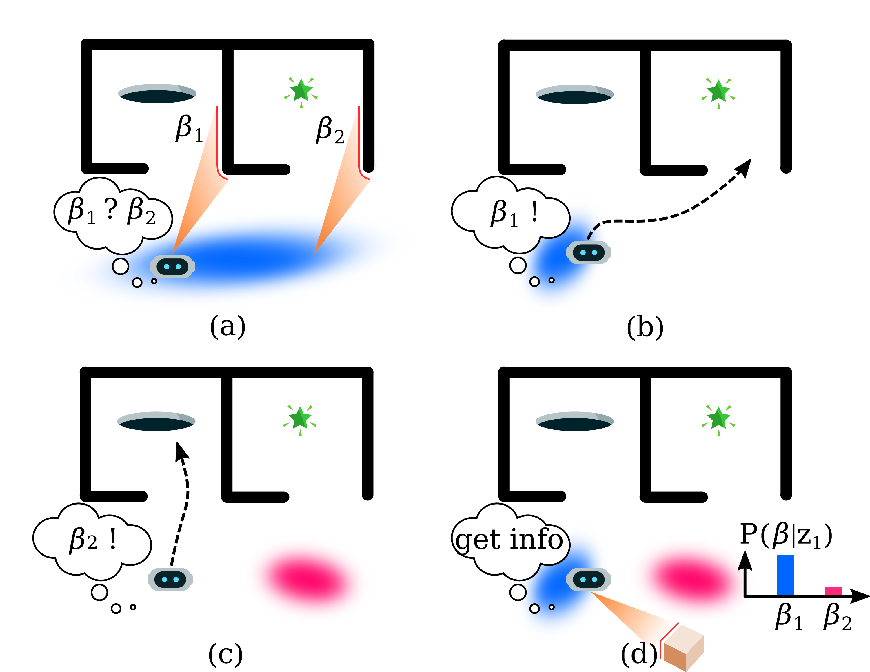
Figure 1: Figure (a) depicts an agent aiming to reach a goal (green star) while receiving an observation that could come from two sources, $\beta_{1}$ or $\beta_{2}$. In Figures (b) and (c), incorrect assumptions about the origin of the observation lead to changes in the robot’s belief (blue and pink ellipses) and the optimal action, which can vary significantly. Notably, in (c), the calculated best action results in unsafe states. Instead, figure (d) showcases a data association aware belief and action, in which the agent holds two distinct hypotheses. Consequently, the agent chooses an action to gather information rather than traveling directly towards the goal.

In general POMDPs, a plan that accounts for uncertainty maintains a distribution over the possible states of the world. Accounting for ambiguous data associations adds another layer of complexity by having to consider multiple hypotheses, leading to a mixture distribution, where each component of the mixture corresponds to a single hypothesis. Additionally, as the planning horizon grows, the number of hypotheses grows exponentially [1], adding a significant computational burden.

In response to the challenges posed by ambiguous data associations in POMDPs, we propose a simplification approach, which maintains a small subset of the hypotheses instead of maintaining an exponential number thereof. Importantly, we derive bounds on the utility function between the POMDP with the simplified and the non-simplified beliefs. We use these bounds to establish a trade-off between computational efficiency and performance for state-dependent rewards. Further, using this relationship, we propose a novel pruning approach that balances computational efficiency with performance loss by adaptively selecting which hypotheses to prune online.

Unlike current state-of-the-art POMDP planners that rely on particle propagation, e.g. POMCP or DESPOT, our proposed approach overcomes the challenge of particle depletion by introducing a novel estimator for the objective function. This estimator is agnostic to the inference mechanism being used, it supports both nonparametric and parametric inference mechanisms to enable long planning horizons. Through experiments in simulated environments, we demonstrate the effectiveness of our proposed approach in handling multi-modal belief hypotheses with ambiguous data associations.

In this paper we make the following main contributions: (a) we derive a theoretical relation between the POMDP with a complete set of hypotheses and the pruned set of hypotheses, enabling us to establish a trade-off between computational efficiency and performance; (b) we develop an estimator that enables parametric and nonparametric belief mixture representation to address particle depletion; (c) we establish a similar relation between an estimated value function based on the complete set of hypotheses and the value function of the pruned set of hypotheses; (d) our bounds can be utilized to provide guarantees in terms of worst-case loss in planning performance given some pruning method; (e) moreover, we derive a scheme that utilizes our bounds to adaptively decide which hypotheses to prune to meet a user-defined allowable loss in planning performance. Finally, we demonstrate the effectiveness of our planning algorithm in a simulated environment with unresolved data associations leading to multi-modal belief. This paper is accompanied by supplementary material [2] that provides proofs for the claims in this paper.

II Related Work

While addressing the challenge of ambiguous data associations (DA) has been extensively researched in the passive inference community, [3, 4, 5, 6], the planning community has had relatively few attempts at supporting ambiguous DA. General state-of-the-art POMDP planners, such as DESPOT, POMCPOW or PFT-DPW [7, 8] do not directly support DA out-of-the-box. Although they can be altered to support DA, e.g. by replacing the observation model with a mixture of observation models, an ad-hoc variation will often result in particle depletion due to the multi-modal nature of a multiple hypotheses belief. Particle depletion results in an overconfident and potentially incorrect action selection due to the low representation of likely state particles in a belief.

A more dedicated approach for handling ambiguous DA could be to explicitly maintain multiple representations of conditional beliefs, each depending on different DA history. A naive attempt to perform planning with all hypotheses results in an exponentially increasing number of hypotheses which is computationally infeasible. Instead, DA-BSP, [1], solves POMDPs by explicitly maintaining hypotheses within the search tree and performs pruning by keeping only a fixed number of the most promising hypotheses, or by keeping only the hypotheses above some threshold on their probabilistic values. However, these pruning methods lack mathematical guarantees and are merely used as a tool to reduce the computational burden. More recently, [9, 10] considered different settings for planning with hypotheses pruning and suggested an algorithm that actively plans to reduce hypotheses ambiguity by defining an objective function over the hypotheses distribution. Their approach provides bounds with respect to that unique objective function and is specifically tailored for that task. Lastly, [11] proposed an adaptive approach that invests computational efforts in the most promising branches of both the planning and hypotheses trees. Their method considers arbitrary state-dependent rewards but comes only with asymptotic guarantees.

III PRELIMINARIES

In this section, we formally define a POMDP with a belief that considers ambiguous data associations. The POMDP $M$ is a tuple $\langle\mathcal{X},\mathcal{A},\mathcal{Z},T,O,R\rangle$, where $\mathcal{X}$, $\mathcal{A}$, and $\mathcal{Z}$ represent the state, action, and observation spaces, respectively. The transition density function $T(x_{t},a_{t},x_{t+1})\triangleq\mathbb{P}({x_{t+1}|x_{t},a_{t}})$ defines the probability of transitioning from state $x_{t}\in\mathcal{X}$ to state $x_{t+1}\in\mathcal{X}$ by taking action $a_{t}\in\mathcal{A}$. The observation density function $O(x_{t},z_{t})\triangleq\mathbb{P}({z_{t}|x_{t}})$ expresses the probability of receiving observation $z_{t}\in\mathcal{Z}$ from state $x_{t}\in\mathcal{X}$.

Given the limited information provided by observations, the true state of the agent is uncertain and a probability distribution function over the state space, also known as a belief, is maintained. The belief depends on the entire history of actions and observations, and is denoted $H_{t}\triangleq\{z_{1:t},a_{0:t-1}\}$. We also define the propagated history as $H_{t}^{-}\triangleq\{z_{1:t-1},a_{0:t-1}\}$. At each time step $t$, the belief is updated using Bayes’ rule and the transition and observation models, given the previous action $a_{t-1}$ and the current observation $z_{t}$, $b\left(x_{t}\right)=\eta_{t}\int\mathbb{P}({z_{t}|x_{t}})\mathbb{P}({x_{t}|x_{t-1},a_{t-1}})b\left(x_{t-1}\right)dx_{t}$, where $\eta_{t}$ denotes a normalization constant and $b_{t}\triangleq\mathbb{P}({x_{t}\mid H_{t}})$ denotes the belief at time t. The updated belief, $b_{t}$ sometimes referred to as the posterior belief, or simply the posterior. We will use them interchangeably throughout the paper.

A policy function $a_{t}=\pi(b_{t})$ determines the action to be taken at time step $t$, based on the current belief $b_{t}$. In the rest of the paper we write $\pi_{t}\equiv\pi(b_{t})$ for conciseness. The reward is defined as an expectation over a state-dependent function, $\rho(b_{t},a_{t})=\mathbb{E}_{x\sim b_{t}}[r_{x}(x,a_{t})]$. The value function for a policy $\pi$ over a finite horizon $\mathcal{T}$ is defined as the expected cumulative reward received by executing $\pi$,

$$V^{\pi}(b_{t})=\rho(b_{t},\pi_{t})+\underset{z_{t+1:T}}{\mathbb{E}}\left[\sum_{\tau=t+1}^{T}\rho(b_{\tau},\pi_{\tau})\right].$$ (1)

The action-value function is defined by executing action $a_{t}$ and then following policy $\pi$ for a finite horizon $T$. The goal of the agent is to find the optimal policy $\pi^{*}$ that maximizes the value function.

III-A Ambiguous Data Associations as Mixture Belief

To represent ambiguous data associations within the POMDP framework we define the belief as a mixture distribution, that encompasses both continuous and discrete random variables. The discrete variables, $\beta_{t}$, represent different associations to seen observations at time $t$. We formally define the mixture belief at each time $t$ as,

$$b\left(x_{t}\right)=\sum_{\beta_{0:t}}\mathbb{P}({\beta_{0:t}\mid H_{t}})\mathbb{P}({x_{t}|\beta_{0:t},H_{t}}),$$ (2)

where $\mathbb{P}({\beta_{0:t}\mid H_{t}})$ is the marginal belief over discrete variables which can be considered as the mixture weight. An hypothesis, $\beta_{0:t}$, denote the entire sequence of associations up to time step $t$. $\mathbb{P}({x_{t}|\beta_{0:t},H_{t}})$ is the conditional belief over continuous variables, given that the history and associations are known. The marginal belief over the hypothesis, $\beta_{0:t}$, can be updated by applying Bayes rule followed by chain rule,

$$\mathbb{P}({\beta_{0:t}\mid H_{t}})=\eta_{t}\mathbb{P}(z_{t}\mid\beta_{0:t},H_{t}^{-})\mathbb{P}(\beta_{0:t}\mid H_{t}^{-})$$ (3)

$$=\eta_{t}\mathbb{P}(z_{t}\mid\beta_{0:t},H_{t}^{-})\mathbb{P}(\beta_{t}\mid\beta_{0:t-1},H_{t}^{-})\mathbb{P}(\beta_{0:t-1}\mid H_{t}^{-}).$$

The conditional belief is updated for each realization of discrete random variables as

$$\mathbb{P}({x_{t}|\beta_{0:t},H_{t}})=\psi\big{(}\mathbb{P}({x_{t-1}|\beta_{0:t-1},H_{t-1}}),a_{t-1},z_{t}\big{)},$$ (4)

where $\psi(.)$ represents the Bayesian inference method. Last, the reward function can now be written in terms of hypothesis dependency, $r(b_{t},a_{t})=\mathbb{E}_{x\sim b_{t}}[r_{x}(x,a_{t})]=\mathbb{E}_{\beta_{0:t}}\left[\mathbb{E}_{x}[r_{x}(x,a_{t})\mid\beta_{0:t}]\right]$. For conciseness, we will denote

$$r(b_{t}^{\beta},\pi_{t})\triangleq\mathbb{E}_{x}[r_{x}(x,a_{t})\mid\beta_{0:t}].$$ (5)

III-B IS and SN estimators

Importance sampling (IS) is a Monte Carlo simulation technique for estimating the expected value of a target function with respect to a probability distribution. The IS estimator involves drawing samples from a proposed distribution and weighting them by the ratio of the target distribution, $\mathbb{P}({\cdot})$ to the proposal distribution, $Q(\cdot)$,

$$\hat{\mathbb{E}}^{IS}\left[r(x)\right]\triangleq\frac{1}{N}\sum_{i=1}^{N}\omega(x^{i})r(x^{i})=\frac{1}{N}\sum_{i=1}^{N}\frac{\mathbb{P}({x^{i}})}{Q(x^{i})}r(x^{i}).$$ (6)

The estimator is unbiased and consistent [12], when the proposal distribution is non-zero wherever the target distribution is non-zero. Self-normalized importance sampling sometimes serves as a lower-variance estimator by normalizing the importance weights. The SN-estimator is described as,

$$\hat{\mathbb{E}}^{SN}\left[r(x)\right]\triangleq\sum_{i=1}^{N}\frac{\omega(x^{i})}{\sum_{j=1}^{N}\omega(x^{j})}r(x^{i}),$$ (7)

which converts the weights to a probability distribution. The SN-estimator is biased, but consistent estimator.

IV PLANNING WITH AMBIGUOUS DATA ASSOCIATIONS

In this section, we provide an overview of our algorithm, DA-MCTS, and the baseline algorithm, vanilla Hybrid Belief-MCTS (HB-MCTS) [11]. To facilitate understanding, we present the pseudo-code for both algorithms jointly in Algorithm 1. We adopt a unified view, with comments indicating the lines unique to each algorithm.

DA-MCTS is built upon the vanilla HB-MCTS algorithm, which itself is an adaptation of PFT-DPW [7] and MCTS [13]. While we have chosen to use these algorithms as the foundation for our work, we acknowledge that other approaches may also be applicable, and we leave exploration of these avenues to future research.

Vanilla HB-MCTS, a variant of belief-Markov Decision Process (BMDP), reframes the POMDP into a belief-state model. In this, states are replaced by belief-states reflecting an agent’s environmental uncertainty. The transition and observation functions update prior to posterior beliefs based on action and observation, mirroring the stochastic state changes in a standard MDP. By transforming POMDP to a BMDP, many MDP planning algorithms, including MCTS, can be used as planning solvers. Notably, single particle propagation algorithms, such as POMCPOW, are also possible, but may suffer from particle depletion as mentioned in section II.

Algorithm 1 presents a pseudo-code for the vanilla HB-MCTS algorithm. In the Simulate procedure, an action is selected based on the Upper Confidence Bound (UCB) heuristic in line 4. Depending on whether the budget on the number of observations has been met, the algorithm either expands a new posterior node, which includes its belief and reward function, and then performs a rollout, or uniformly samples an existing posterior node and continues recursively to the next node. Finally, the action value of the current node and its relevant counters are updated. The vanilla HB-MCTS algorithm is flexible in that the number of maintained posterior hypotheses can be controlled and remain fixed based on a pre-defined hyperparameter. For instance, a vanilla HB-MCTS with low compute resources can have a pruning budget, where only $K$ hypotheses are maintained in each node of the planning tree. The pruned hypotheses are usually chosen heuristically, e.g. based on their probability value.

However, Vanilla HB-MCTS is limited in its ability to provide guarantees when pruning is performed. While the performance guarantees we present in the next section are applicable to any pruning heuristic, such as the one used in vanilla HB-MCTS, we introduce a slightly different approach. Instead of pre-defining a fixed number of hypotheses to maintain, we propose an adaptive approach that determines which hypotheses to prune online based on a pre-defined maximum allowable loss, $\epsilon_{\bar{D}}$. We then modify the HB-MCTS algorithm to adaptively determine which hypotheses to prune, while maintaining performance guarantees with respect to the complete set of hypotheses. This modification is reflected in line 7.

In addition, DA-MCTS can provide even tighter guarantees in hindsight without incurring additional computational complexity, denoted by $\hat{\epsilon}^{hs}_{\bar{D}}$, shown in line 18. The increased accuracy of these guarantees is due to the granularity of the hypotheses weights. For instance, when there is only a single hypothesis, no hypotheses are pruned, resulting in zero additional loss to the value function. The specific bounds and estimators used are discussed in the following section.

Algorithm 1 HB-MCTS and DA-MCTS

Procedure:Simulate($b,h,d,\epsilon_{\bar{D}}$)
/*Init: $N(b),N(ba),Q(ba),\hat{\epsilon}_{\bar{D}}^{hs}(b),\hat{\delta}_{\bar{D}}^{\beta}(b)$ to $0$*/

1: if d = 0 then

2:    return  0

3: end if

4: $a\xleftarrow{}\underset{\bar{a}}{\arg\max}\ Q(b\bar{a})+c\sqrt{\frac{log(N(b))}{N(b\bar{a})}}$

5: if $|C(ba)|\leq k_{o}N(ba)^{\alpha_{o}}$  then

6:     $b^{\prime}\xleftarrow{}$ PrunedPosterior$(b,a)$ /*Vanilla HB-MCTS*/

7:     $b^{\prime},\delta_{\bar{D}}^{\beta}\xleftarrow{}$ PruningWithGuarantees$(b,a,\epsilon_{\bar{D}})$ /*DA-MCTS. Eq. (13)*/

8:    $r\xleftarrow{}$ Reward$(b,a)$

9:    $C(ba)\cup\{(b^{\prime},r)\}$

10:    $R\xleftarrow{}r+$Rollout$(b^{\prime},d-1)$

11: else

12:    $b^{\prime},r\xleftarrow{}$ Sample uniformly from $C(ba)$

13:    $R$, $\hat{\epsilon}_{\bar{D}}^{hs}$$\xleftarrow{}r+$Simulate$(b^{\prime},d-1,\epsilon_{\bar{D}})$

14: end if

15: $N(b)\xleftarrow{}N(b)+1$

16: $N(ba)\xleftarrow{}N(ba)+1$

17: $Q(ba)\xleftarrow{}Q(ba)+\frac{R-Q(ba)}{N(ba)}$

18:  $\hat{\epsilon}_{\bar{D}}^{hs}\xleftarrow{}$ GetGuarantees$(\hat{\epsilon}_{\bar{D}}^{hs},\hat{\delta}_{\bar{D}}^{\beta})$ /*DA-MCTS. Eq. (12)*/

19: return $R$, $\hat{\epsilon}_{\bar{D}}^{hs}$

V Mathematical analysis

In this section, we mathematically analyze the impact of pruning on the performance of the agent. We establish a novel relationship between the complete and pruned value functions for state-dependent reward functions and provide bounds on the loss of approximation. Due to restricted space we defer most proofs and derivations to the supplementary file [2].

We define $D_{t}=\{\beta_{t}^{1},\beta_{t}^{2},...,\beta_{t}^{|D_{t}|}\}$ the set of associations at time step $t$, and $\overline{D}_{t}\subseteq D_{t}$ as the subset of hypotheses survived after the pruning procedure. We define the pruned belief as,

$$\overline{b}_{t}\triangleq\bar{\mathbb{P}}(x_{t}\mid H_{t})=\sum_{\beta_{t}\in\overline{D}_{t}}\mathbb{P}(x_{t}\mid\beta_{t},H_{t})\bar{\mathbb{P}}(\beta_{t}\mid H_{t}),$$ (8)

where the $\bar{\square}$ notation indicates a pruned distribution after normalization. This can be explicitly written as,

$$\overline{b}_{t}=\!\!\!\!\int\limits_{x_{t-1}}\!\!\!\overline{b}_{t-1}\frac{\sum_{\beta_{t}\in\overline{D}_{t}}\mathbb{P}(z_{t}\mid x_{t},\beta_{t})\mathbb{P}(\beta_{t}\mid x_{t})\mathbb{P}(x_{t}\mid x_{t-1},\pi_{t-1})}{\overline{\mathbb{P}}\left(z_{t}\mid H_{t}^{-}\right)},$$ (9)

where, $\overline{\mathbb{P}}\left(z_{t}\mid H_{t}^{-}\right)=\int_{x_{t-1:t}}\sum_{\beta_{t}\in\overline{D}_{t}}\mathbb{P}(z_{t}\mid x_{t},\beta_{t})\mathbb{P}(\beta_{t}\mid x_{t})\mathbb{P}(x_{t}\mid x_{t-1},\pi(z_{t-1}))\overline{b}_{t-1}$. Note that the summation is over the pruned set of hypotheses.

Theorem 1

Let time-step $0$ denote the root of the planning tree. Then, the expected reward for the pruned POMDP, $\overline{M}$, is bounded with respect to the full POMDP, $M$, through the factor of the pruned weight values, and the maximum immediate reward,

$$\Bigl{|}\mathbb{E}[r(b_{t},a_{t})]\!-\!\overline{\mathbb{E}}[r(\overline{b}_{t},a_{t})]\Bigr{|}\!\leq\!\mathcal{R}_{max}\left[\delta_{0}^{\beta}\!+\!\!\!\sum_{\tau=1}^{t-1}\overline{\mathbb{E}}_{z_{1:\tau}}\!\!\left[\delta^{\beta}_{\tau}\right]\right],$$ (10)

where $\delta^{\beta}_{\tau}\triangleq\sum_{\beta_{\tau}\in D_{\tau}\backslash\overline{D}_{\tau}}\overline{\mathbb{P}}(\beta_{\tau}\mid H_{\tau})$, i.e. the sum of pruned hypotheses weights at time-step $\tau$.

Crucially, in order to calculate the value of $\delta_{\tau}^{\beta}$, the values of the hypotheses weights which are descendent of past pruned hypotheses are not required, as they cannot be obtained without explicitly calculating all hypotheses. More formally, $\overline{\mathbb{P}}(\beta_{t}\mid H_{t})=\frac{\mathbb{P}(z_{t}\mid\beta_{t},H_{t}^{-})\sum_{\beta_{0:t-1}\in\overline{D}}\mathbb{P}(\beta_{t}\mid\beta_{0:t-1},H_{t-1})\mathbb{P}(\beta_{0:t-1}\mid H_{t}^{-})}{\overline{\mathbb{P}}(z_{t}\mid H_{t}^{-})}$ has summation only over the survived hypotheses.

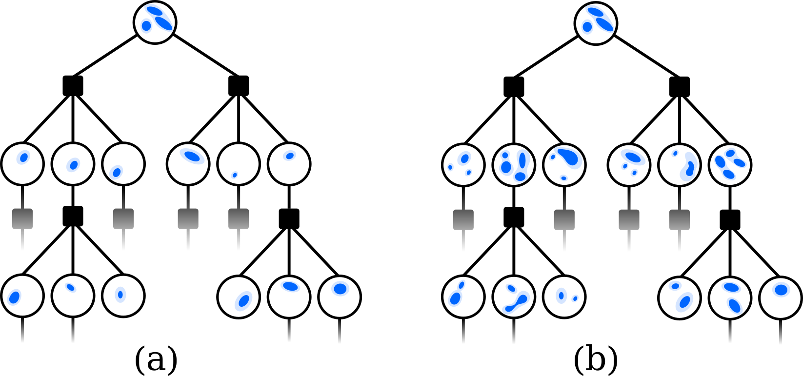
Figure 2: Planning trees with nodes representing beliefs, and inner blue shapes illustrate distributions of the conditional posteriors. (a) A belief tree with standard Monte-Carlo estimator leads to an overconfident, fully observed data association after a single step. (b) A planning tree with Self-Normalized Importance Sampling estimators to account for different hypotheses at posterior nodes.

The generalization of theorem 1 to the entire value function, is straightforward due to linearity of the expectation,

Corollary 1.1

Without loss of generality, assume that the time step at the root node of the planning tree is $t=0$. Then, for any policy $\pi$, the following holds,

$$\left|V^{\pi}(b_{0})\!-\!\bar{V}^{\pi}(\bar{b}_{0})\right|\!\leq\!\mathcal{R}_{max}\!\left[T\delta^{\beta}_{0}\!+\!\sum_{k=1}^{T}\sum_{\tau=1}^{k}\overline{\mathbb{E}}_{z_{1:\tau}}\!\left[\delta^{\beta}_{\tau}\right]\right].$$ (11)

For conciseness, we denote this bound as $\epsilon_{\bar{D}}^{hs}$. As we will derive in the following sections, an equivalent bound can be derived for estimated value functions, that is,

$$|\hat{V}^{{\pi}}(\hat{b}_{0})-\hat{\bar{V}}^{{\pi}}(\hat{\bar{b}}_{0})|\leq\mathcal{R}_{max}\!\left[T\hat{\delta}^{\beta}_{0}\!+\!\sum_{k=1}^{T}\sum_{\tau=1}^{k}\hat{\overline{\mathbb{E}}}_{z_{1:\tau}}\!\left[\hat{\delta}^{\beta}_{\tau}\right]\right],$$ (12)

where $\hat{\square}$ denotes an estimator. Similarly, we denote $\hat{\epsilon}_{\bar{D}}^{hs}$ as the (deterministic) bound for the estimated value functions.

V-A Adaptive Pruning with Performance Guarantees

The theoretical value bound in Equation (11) and the estimator value bound in Equation (12) can be used to provide guarantees for various pruning heuristics, including those presented in prior work such as [1, 11] by providing guarantees after the planning session has ended.

In this section, we go a step further, and propose a novel mechanism for selecting the surviving hypotheses. Unlike previous approaches that use a fixed budget on the number of allowed hypotheses [1], our algorithm requires the user to specify the maximum allowable loss, $\epsilon_{\bar{D}}$, on the value function. Using this allowable loss, our algorithm dynamically selects the cardinality and instances of hypotheses to prune online, while maintaining the performance guarantees provided in advance.

To achieve this, we set the value of $\epsilon_{\bar{D}}$ and by construction determine $\delta^{\beta}_{\tau}$ to be a constant, denoted as $\Delta$, for all $H_{\tau}$ and all time steps $\tau$. We use $\Delta$ to determine which hypotheses to prune in order to meet the budget. The resulting bound can then be expressed as follows,

$$\left|V^{\pi}(b_{0})-\bar{V}^{\pi}(\bar{b}_{0})\right| \leq\mathcal{R}_{max}\Delta\!\left[T+\sum_{k=1}^{T}\sum_{\tau=1}^{k}1\right]$$ (13)

$$=\mathcal{R}_{max}\Delta\left[\frac{T^{2}+3T}{2}\right]\triangleq\epsilon_{\bar{D}}.$$

The hyperparameter $\epsilon_{\bar{D}}$ controls the maximum allowable loss and is set a priori, as a result $\Delta$ can easily be derived. During planning, we sum over $\delta^{\beta}_{\tau}$, until its value is as close as possible to $\Delta$ without crossing its value. The difference between these two values allows us to obtain a tighter guarantee in hindsight, $\epsilon^{hs}_{\bar{D}}$, which satisfies the inequality $\epsilon^{hs}_{\bar{D}}\leq\epsilon_{\bar{D}}$. A similar claim can be made for the sampling-based bound. The formal derivation of these estimators is presented in the next section.

V-B Estimated expected reward

In this section, we first develop an estimator for the value function, assuming the availability of a complete set of hypotheses at each posterior belief. Then, we derive a similar, pruning-based estimator. In the next section, we will show a deterministic relation between the estimators. However, before delving into the details, we first give a motivation for deriving guarantees with respect to the estimators.

As stated in Corollary 1.1, the value function based on the complete set of hypotheses should not deviate significantly from the value function based on the pruned hypotheses set, as long as the pruned hypotheses have low weight values. However, in practice, current state-of-the-art algorithms cannot compute the full nor the pruned value functions due to intractable integrals involved with expectations. Online POMDP algorithms provide performance guarantees based on estimated value functions, where a sampled set of observations and states approximate expectations and the belief distribution, e.g., [14, 15].

For clarity, we derive the estimator by considering separately each expected reward along the planning horizon. Using linearity of the expectation, the value function may be written as,

$$V^{\pi}(b_{0})=\rho(b_{0},\pi_{0})+\sum_{t=1}^{T}\mathbb{E}_{z_{1:t}}[\rho(b_{t},\pi_{t})].$$ (14)

We handle each term in the summation individually, and make the following proposition as a first step towards deriving an estimated expected reward,

Proposition 1

Let $z_{1:t}$ denote an observation sequence, $\rho(b_{t},\pi_{t})$ be the reward value for a given belief, $b_{t}$ and policy $\pi_{t}$. The expected reward value can be written as,

$$\mathbb{E}_{z_{1:t}}[\rho(b_{t},\pi_{t})]=$$ (15)

$$\int_{z_{1:t}}\mathbb{E}_{\beta_{0}}\prod_{\tau=1}^{t}\mathbb{E}_{\beta_{\tau}\mid\beta_{0:\tau-1}}\left[\mathbb{P}\left(z_{\tau}\mid\beta_{0:\tau},H_{\tau}^{-}\right)r\left(b_{t}^{\beta},\pi_{t}\right)\right],$$

where $r\left(b_{t}^{\beta},\pi_{t}\right)$ denotes the reward value of a single hypothesis realization, $\beta_{0:t}$, as shown in equation (5).

From the proposition we derive a standard Monte-Carlo sampling approach, where we iteratively sample sequences of hypotheses $\beta_{0:t}$ and observation samples, $z_{1:t}$,

$$\hat{\mathbb{E}}^{MC}_{z_{1:t}}[\rho(\hat{b}_{t},\pi_{t})]=\frac{1}{N}\sum_{i}\hat{r}\left(b_{t}^{\beta^{i}},\pi_{t}\right),$$ (16)

where $\square^{MC}$ denotes Monte-Carlo estimation and $b_{t}^{\beta^{i}}\triangleq\mathbb{P}\left(x_{t}\mid\beta_{0:t}^{i},z_{1:t}^{i},\pi_{0:t-1}\right)$. However, since the observation space is continuous, different realizations of $\beta_{0:t}$, denoted $\beta_{0:t}^{i}$, will never sample the same observation sequence $z_{1:t}^{i}$ twice. In the planning tree, it means that after an observation sample, there is only a single hypothesis in any posterior node, resulting in a fully observed data association. However, if the agent obtains an observation in the real world, the data association ambiguity is generally not fully resolved. A result, the Monte Carlo sampling approach is an over-optimistic, erroneous planner which only considers ambiguity at the root node of the planning tree. See figure 2 for an illustration.

Inspired by [7] for standard POMDPs, and [11] for hybrid POMDPs, we derive an Importance Sampling (IS) estimator, which may sample observations from different distributions, and weigh each hypothesis with an importance weight, $\omega\left(z_{\tau}\right)$. The importance weight reflects the probability of observing $z_{t}$ given hypothesis $\beta_{0:\tau}$ and history $H_{\tau}^{-}$, normalized to the actual sampling distribution being used, $Q(\cdot)$. We may write equation (15) to reflect the change,

$$\mathbb{E}_{z_{1:t}}[\rho(b_{t},\pi_{t})]=$$ (17)

$$\int_{z_{1:t}}\mathbb{E}_{\beta_{0}}\prod_{\tau=1}^{t}Q\left(z_{\tau}\mid H_{\tau}^{-}\right)\mathbb{E}_{\beta_{\tau}\mid\beta_{0:\tau-1}}\left[\omega\left(z_{\tau}\right)r\left(b_{t}^{\beta},\pi_{t}\right)\right]$$

where $\omega\left(z_{\tau}\right)=\frac{\mathbb{P}\left(z_{\tau}\mid\beta_{0:\tau},H_{\tau}^{-}\right)}{Q\left(z_{\tau}\mid H_{\tau}^{-}\right)}$ and $Q(.)$ is the proposal distribution from which the sampling-based estimator will sample observations. Clearly, the two terms are equivalent. From (17) we can directly derive the IS-estimator,

$$\hat{\mathbb{E}}^{IS}_{z_{1:t}}[\rho(\hat{b}_{t})]=\hat{\mathbb{E}}_{z_{1:t}}\mathbb{E}_{\beta_{1:t}}[\hat{r}\left(b_{t}^{\beta},\pi_{t}\right)]\triangleq$$ (18)

$$\sum_{z_{1:t}^{c}}\!\sum_{\beta_{0:t}\in D_{0:t}}\!\!\!\!\mathbb{P}(\beta_{0})\prod_{\tau=1}^{t}\mathbb{P}\left(\beta_{\tau}\mid\beta_{0:\tau-1},H_{\tau}^{-}\right)\frac{\omega\left(z_{\tau}^{c}\right)}{N}\hat{r}\left(b_{t}^{\beta},\pi_{t}\right)\!,$$

where, $\hat{r}(b_{t}^{\beta},\pi_{t})$ is the sample-based mean for the state-reward over the conditional belief, as defined in equation (5). In contrast to the standard Monte-Carlo estimator (16), using an importance sampling estimator enables us to reason about all hypotheses for every observation sequence, shown by the summation over $\beta_{0:t}$ for each sampled $z_{1:t}^{c}$.

Although the IS estimator is theoretically justified as a consistent and unbiased estimator, we make another step in deriving the estimator and use a Self-Normalized Importance Sampling (SN) estimator,

$$\hat{\mathbb{E}}^{SN}_{z_{1:t}}[\rho(\hat{b}_{t})]=\hat{\mathbb{E}}_{z_{1:t}}\mathbb{E}_{\beta_{1:t}}[\hat{r}\left(b_{t}^{\beta},\pi_{t}\right)]\triangleq$$ (19)

$$\sum_{z_{1:t}^{c}}\!\!\sum_{\beta_{0:t}\in D_{0:t}}\!\!\!\!\!\mathbb{P}(\beta_{0})\!\!\prod_{\tau=1}^{t}\!\mathbb{P}({\beta_{\tau}|\beta_{0:\tau-1},H_{\tau}^{-}})\frac{\omega\left(z_{\tau}^{c}\right)}{\sum_{z_{\tau}^{k}}\omega\left(z_{\tau}^{k}\right)}\hat{r}\left(\!b_{t}^{\beta},\pi_{t}\!\right)$$

The SN-estimator is no longer unbiased, but is known to be consistent [12]. The main reason for that step is to achieve a bounded deterministic difference between the full and pruned estimators, as we will describe in the following section.

Last, we derive a similar estimator for the pruned posterior belief,

$$\hat{\overline{\mathbb{E}}}_{z_{1:t}}\left[\rho\left(\hat{\overline{b}}_{t},\pi_{t}\right)\right]=\hat{\mathbb{E}}_{z_{1:t}}\bar{\mathbb{E}}_{\beta_{1:t}}[\hat{r}\left(b_{t}^{\beta},\pi_{t}\right)]\triangleq$$ (20)

$$\sum_{z_{1:t}^{c}}\!\!\sum_{\beta_{0:t}\in\overline{D}_{0:t}}\!\!\!\!\!\mathbb{P}(\beta_{0})\!\!\prod_{\tau=1}^{t}\!\mathbb{P}({\beta_{\tau}\mid\beta_{0:\tau-1},H_{\tau}^{-}})\frac{\omega\left(z_{\tau}^{c}\right)}{\sum_{z_{\tau}^{k}}\omega\left(z_{\tau}^{k}\right)}\hat{r}\left(\!b_{t}^{\beta},\pi_{t}\!\right)\!.$$

V-C Estimators analysis

In this section, we derive a bounded relationship between the full and pruned estimators. Finally, we discuss how these estimators relate to the theoretical value function.

Theorem 2

Let $\pi$ be a policy, then the expected reward for the estimated pruned POMDP, $\hat{\overline{M}}$, is bounded with respect to the estimated full POMDP, $\hat{M}$, as follows,

$$\left|\hat{\mathbb{E}}^{\pi}_{z_{1:t}}[\rho(\hat{b}_{t})]-\hat{\overline{\mathbb{E}}}^{\pi}_{z_{1:t}}\left[\rho\left(\hat{\overline{b}}_{t}\right)\right]\right|\!\leq\!\mathcal{R}_{max}\left[\hat{\delta}_{0}^{\beta}\!+\!\sum_{\tau=1}^{t}\hat{\delta}_{\tau}^{\beta}\right]\!.$$ (21)

where, $\hat{\delta}_{\tau}^{\beta}=\hat{\mathbb{E}}_{z_{1:t}^{c}}\overline{\mathbb{E}}_{\beta_{0:t-1}}\sum_{\beta_{t}\in D_{t}\backslash\overline{D}_{t}}\mathbb{P}\left(\beta_{t}\mid\beta_{0:t-1},H_{t}^{-}\right)$ for all $\tau\in[1,t]$ represents the expected sum of conditional hypotheses’ weights which are myopically pruned and $\hat{\delta}_{0}^{\beta}=\sum_{\beta_{0}\in D_{0}\backslash\overline{D}_{0}}\mathbb{P}\left(\beta_{0}\mid H_{t}^{-}\right)$.

In accordance with the theoretical case, as described in Equation (17), to evaluate $\hat{\delta}_{\tau}^{\beta}$, only the surviving hypotheses from past time steps are needed. The theorem can be generalized to the full value function by re-introducing the summation. Under the assumptions of theorem 2 the following holds,

Corollary 2.1

The difference between the estimated value function of the full POMDP, $\hat{M}$, and the estimated value function of the pruned POMDP, $\hat{\overline{M}}$, is bounded by,

$$|\hat{V}^{{\pi}}(\hat{b}_{0})-\hat{\bar{V}}^{{\pi}}(\hat{\bar{b}}_{0})|\leq\mathcal{R}_{max}\left[T\hat{\delta}^{\beta}_{0}+\sum_{k=1}^{T}\sum_{\tau=1}^{k}\hat{\delta}^{\beta}_{\tau}\right].$$ (22)

The corollary relates the complete but computationally expensive value function estimator to the efficient, pruning-based estimator. Both estimators utilize the same sampled observations since they share the same proposal distribution.

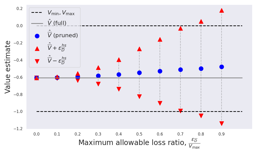
(a)

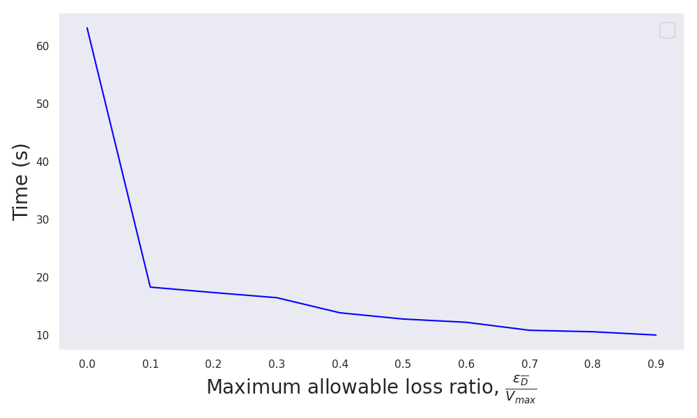
(b)

Figure 3: (a) Bounds of our approach with respect to level of simplification. $\hat{V},\hat{\bar{V}}$ are the value functions of the full and pruned estimators respectively. $\hat{\bar{V}}+\hat{\epsilon}_{\bar{D}}^{hs}$ represent the bounds of the pruned estimator. $V_{\min},\backslash V_{\max}$ represent the minimum and maximum theoretical values of the value function. All values are normalized with respect to $\max\{\left|V_{min}\right|,\left|V_{max}\right|\}$. Here $\left|V_{max}\right|\equiv 0$ since the reward is defined as the negative Euclidean distance to goal. (b) Time for task completion with respect to level of simplification. Each level corresponds to the bounds presented in figure (a).

Finding a finite sample algorithm with practical guarantees between the estimated value function and the theoretical remains an open challenge in the POMDP literature and is aside from our current contribution. Nevertheless, to fully justify our approach, we formally state that given such an algorithm, denoted $\mathcal{A}$, that utilizes the importance sampling estimator defined in equation (19), our simplified estimator provides a relationship to the theoretical value function while being more efficient,

Corollary 2.2

Let $\pi$ be a policy and let $\mathcal{A}$ be a sampling-based estimator for the value function such that $|V^{\pi}(b_{0})-\hat{V}^{\pi}(\hat{b}_{0})|\leq\epsilon_{\mathcal{A}}$ with probability at least $1-\delta_{\mathcal{A}}$. Then, the loss in the value function for the pruned hypotheses is bounded,

$$|V^{\pi}(b_{0})-\hat{\bar{V}}^{{\pi}}(\hat{\bar{b}}_{0})|\leq$$ (23)

$$|V^{\pi}(b_{0})-\hat{V}^{{\pi}}(\hat{b}_{0})|+|\hat{V}^{{\pi}}(\hat{b}_{0})-\hat{\bar{V}}^{{\pi}}(\hat{\bar{b}}_{0})|\leq\epsilon_{\mathcal{A}}\!+\hat{\epsilon}^{hs}_{\bar{D}},$$ (24)

and holds with probability $1-\delta_{\mathcal{A}}$. We use $\hat{\epsilon}^{hs}_{\bar{D}}$ as a shorthand for the bounds provided in corollary 2.1.

The results established so far hold for any policy, assuming that both the theoretical and estimated value functions are based on the same policy. However, planning based on the pruned belief may result in a different policy from the optimal one for the underlying POMDP. Nevertheless, we demonstrate that the optimal policy for the pruned and potentially sampled-based POMDP, denoted $\bar{\pi}$, incurs bounded loss in performance compared to the optimal policy for the full theoretical POMDP, denoted $\pi^{\star}$.

Corollary 2.3

Let $\bar{\pi}$ be the optimal policy for the pruned, possibly sampled-based POMDP and $\pi^{\star}$ be the optimal policy for the full theoretical POMDP. Then,

$$\left|V^{\pi^{\star}}(b_{t})-\hat{\bar{V}}^{\bar{\pi}}(\hat{\bar{b}}_{t})\right|\leq{\color[rgb]{0,0,0}2}\left(\epsilon_{\mathcal{A}}+\hat{\epsilon}^{hs}_{\bar{D}}\right).$$ (25)

This is an unsurprising result, since the best policy for the pruned approximation, $\bar{\pi}$, should perform no worse than the optimal policy, $\pi^{\star}$, for the simplified POMDP or otherwise it would have been selected.

VI EXPERIMENTS

In this section we experiment with different pruning approaches to validate our findings. We use MCTS as a baseline algorithm and compare multiple hypothesis pruning approaches to our adaptive scheme. The experimental evaluation of our approach consists of two main parts. In the first part, we validate the proposed bounds and investigate their sensitivity to the level of simplification chosen. In the second part, we conduct a simulation study to demonstrate the practical performance gains of our adaptive pruning approach.

Importantly, we emphasize that the theoretical guarantees presented in section V are suitable for other hypotheses-based algorithms as well, such as [1, 11] or PFT-DPW [7] if the latter is adapted to multiple hypotheses.

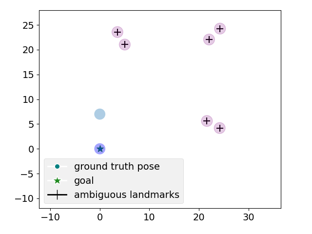
(a)

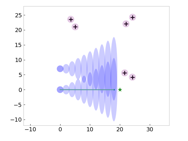
(b)

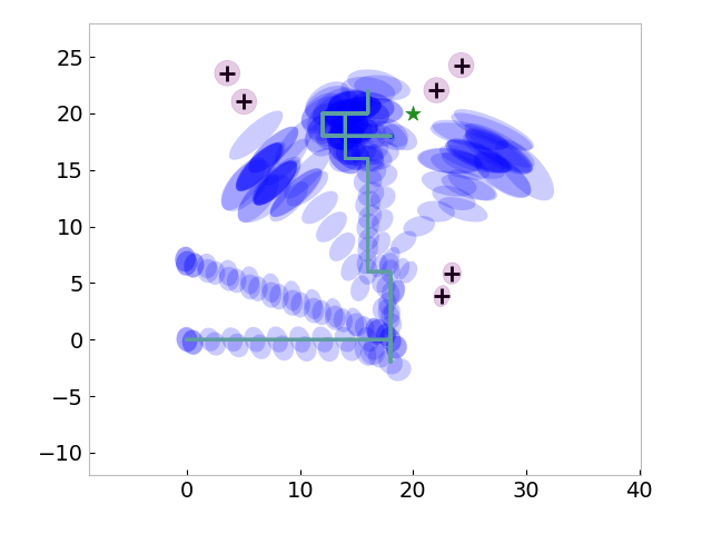
(c)

Figure 4: The figures demonstrate the estimated state of the entire trajectory, also known as the smoothing state, of the agent at time $t$ given the observed history. (a) The prior of the agent given as two Gaussian hypotheses. Each Gaussian represented as an ellipse illustrating its Covariance, centered around its mean. The landmarks are part of the agent state a-priori but has an uncertain location, with ellipses illustrating their Covariances. (b) The belief of the agent adjacent to the first waypoint before obtaining any observation. (c) The belief of the agent after pruning. Non negligible hypotheses differ substantially.

To conduct the simulations, we utilized the GTSAM library [16] as our inference engine. Our belief model is based on a Gaussian Mixture Model, in which each posterior belief in the planning tree corresponds to multiple instances of GTSAM factor graphs. Each instance represents a conditional posterior over the continuous part of the belief, $\mathbb{P}({x_{t}\mid\beta_{0:t},H_{t}})$, while the discrete part of the belief, $\mathbb{P}({\beta_{0:t}\mid H_{t}})$, is maintained as a list of probability values, each corresponds to an hypothesis. Apart from the pruning method, which is the focus of this section, all hyper-parameters are shared across all solvers and remain fixed. The planning is performed in a receding horizon manner, where after each planning session, only the first action is executed, and all calculations are done from scratch in the subsequent step.

In the first experiment the belief of the agent included the pose of the agent and two ambiguous landmarks. The objective of the agent was to reach a target destination, encoded into the reward function as the expected Euclidean norm between the agent pose samples and the target. The field of view of the agent was chosen to be unbounded and with unlimited sensing range, that is, at every time step, the agent obtains an observation from two sources, but cannot identify its source. In this simple toy example, the number of hypotheses quickly grows and becomes intractable due to the exponential nature of the problem. Given a horizon of 10 steps, the number of hypotheses becomes $D_{10}=2^{10}$, each is a Gaussian conditional distribution. In this and the next experiments the action space is defined as primitive actions, up-down-left-right, in a fixed step size.

The estimated value function obtained from the complete set of hypotheses and the simplified estimator generated using the adaptive pruning approach, as outlined in Section V, are illustrated in figure 3. The solver was endowed with an a-priori budget, limiting the maximum loss, denoted as $\epsilon_{\overline{D}}$. Based on the estimator value, the solver determined online which hypotheses to prune and which to retain.

The results indicate that, as the bounds become looser, i.e., when the value of $\epsilon_{\overline{D}}$ increases, the computation time efficiency also increases, trading off efficiency with performance. As the bounds increases beyond the value of $0.7$, they become uninformative since the bounds are larger or smaller than $V_{\max},V_{\min}$, respectively. On the other hand, when the allowable loss budget was set to zero, no hypotheses were pruned, resulting in identical value estimations for both the pruned and the full estimators, which leads to an identical result as the baseline method of no pruning.

In the second experiment, we aimed to compare the ability of different pruning schemes to complete the task under a limited time-budget of 20 seconds, identical to all solvers. Specifically, we compare the performance of our approach to three types of pruning baselines; no pruning (Full-HB-MCTS), maintaining a fixed number of hypotheses (K-HB-MCTS) and pruning below a threshold value (P_thresh-HB-MCTS). Notably, P_thresh-HB-MCTS can be seen as an extension of DA-BSP [1], to an MCTS-based algorithm instead of Sparse Sampling, as the earlier is known to perform empirically better. For each pruning method we have experimented with multiple hyperparameters, P${}_{thresh}\in\{0.01,0.1,0.3\}$ for P_thresh-HB-MCTS, K$\in\{1,3,10\}$ for K-HB-MCTS, and $\frac{\epsilon_{\overline{D}}}{V_{\max}}\in\{0.1,0.2,0.5\}$ for DA-MCTS. The best are shown in Table I.

In that experiment, the goal of the agent was to reach an ordered set of waypoints , positioned on coordinates $[20,0],[20,20],[0,20]$, see figure 4 for an illustration. After performing 60 steps in the environment, the simulation was restarted. The reward was defined as the expected sum of distance to the next waypoint. The state space was defined as the agent pose, and the positions of the landmarks. Ambiguous landmarks were placed in the vicinity of each waypoint to challenge the solvers by causing an exponential increase in the number of hypotheses.

The results of this experiment are presented in Table I. Our findings indicate that the performance of the HB-MCTS algorithm improved when the number of hypotheses was reduced. Given the allocated time budget, maintaining a large set of hypotheses significantly impeded efficiency, leading to a degradation of the planner’s exploration. Conversely, maintaining a single hypothesis resulted in an overconfident solver that potentially relied on the wrong association sequence. Our proposed algorithm performed comparably well, as it was able to distinguish between hypotheses with a significant impact on the value function and those with low impact, which can be pruned.

TABLE I: Reaching waypoints performance over 10 trials. The pruning hyperparameters chosen for the experiments are $(K=1,$P${}_{thresh}=0.1,\frac{\epsilon_{\overline{D}}}{V_{\max}}=0.2)$ for K-HB-MCTS, P_thresh-HB-MCTS and DA-MCTS respectively.

Algorithm	Waypoint 1	Waypoint 2	Waypoint 3
DA-MCTS (ours)	100.0%	100.0%	90.0%
Full-HB-MCTS	100.0%	$30.0$%	$20.0$%
K-HB-MCTS	100.0%	$80.0$%	$60.0$%
Pthresh-HB-MCTS	100.0%	$80.0$%	$60.0$%

VII CONCLUSIONS

This paper proposes a pruning-based approach for efficient autonomous decision-making in environments with ambiguous data associations. The approach models the data association problem as a partially observable Markov decision process (POMDP) and represents multiple data association hypotheses as a belief mixture. The challenge of handling the exponential growth in the number of hypotheses was addressed by pruning the hypotheses while planning, with the number of hypotheses being adapted based on bounds derived on the value function.

The results of our evaluations in simulated environments demonstrate the effectiveness of our approach in handling multi-modal belief hypotheses with ambiguous data associations. Our method provides a practical solution for autonomous agents to make decisions in environments with partial observability and guaranteed performance.

Future research goals include extending the bounds to hybrid belief use-cases, improving solver scalability for ambiguous data associations, efficient recovery of lost hypotheses, and exploring computational burden reduction techniques like merging hypotheses with guarantees.

References

- [1] S. Pathak, A. Thomas, and V. Indelman, “A unified framework for data association aware robust belief space planning and perception,” Intl. J. of Robotics Research, vol. 32, no. 2-3, pp. 287–315, 2018.
- [2] M. Barenboim, I. Lev-Yehudi, and V. Indelman, “Data association aware pomdp planning with hypothesis pruning performance guarantees - supplementary material,” Technion - Israel Institute of Technology, Tech. Rep. [Online]. Available: https://tinyurl.com/2fekv2pu
- [3] C. Cadena, L. Carlone, H. Carrillo, Y. Latif, D. Scaramuzza, J. Neira, I. D. Reid, and J. J. Leonard, “Simultaneous localization and mapping: Present, future, and the robust-perception age,” IEEE Trans. Robotics, vol. 32, no. 6, pp. 1309 – 1332, 2016.
- [4] D. Fourie, J. Leonard, and M. Kaess, “A nonparametric belief solution to the bayes tree,” in IEEE/RSJ Intl. Conf. on Intelligent Robots and Systems (IROS), 2016.
- [5] V. Tchuiev, Y. Feldman, and V. Indelman, “Data association aware semantic mapping and localization via a viewpoint-dependent classifier model,” in IEEE/RSJ Intl. Conf. on Intelligent Robots and Systems (IROS), 2019.
- [6] K. Doherty, D. Fourie, and J. Leonard, “Multimodal semantic slam with probabilistic data association,” in 2019 international conference on robotics and automation (ICRA). IEEE, 2019, pp. 2419–2425.
- [7] Z. Sunberg and M. Kochenderfer, “Online algorithms for pomdps with continuous state, action, and observation spaces,” in Proceedings of the International Conference on Automated Planning and Scheduling, vol. 28, no. 1, 2018.
- [8] A. Somani, N. Ye, D. Hsu, and W. S. Lee, “Despot: Online pomdp planning with regularization.” in NIPS, vol. 13, 2013, pp. 1772–1780.
- [9] M. Shienman and V. Indelman, “D2a-bsp: Distilled data association belief space planning with performance guarantees under budget constraints,” in IEEE Intl. Conf. on Robotics and Automation (ICRA), 2022.
- [10] ——, “Nonmyopic distilled data association belief space planning under budget constraints,” in Proc. of the Intl. Symp. of Robotics Research (ISRR), 2022.
- [11] M. Barenboim, M. Shienman, and V. Indelman, “Monte carlo planning in hybrid belief pomdps,” IEEE Robotics and Automation Letters, vol. 8, no. 8, pp. 4410–4417, 2023.
- [12] A. Doucet, N. de Freitas, and N. Gordon, Eds., Sequential Monte Carlo Methods In Practice. New York: Springer-Verlag, 2001.
- [13] L. Kocsis and C. Szepesvári, “Bandit based monte-carlo planning,” in European conference on machine learning. Springer, 2006, pp. 282–293.
- [14] D. Silver and J. Veness, “Monte-carlo planning in large pomdps,” in Advances in Neural Information Processing Systems (NIPS), 2010, pp. 2164–2172.
- [15] M. H. Lim, T. J. Becker, M. J. Kochenderfer, C. J. Tomlin, and Z. N. Sunberg, “Generalized optimality guarantees for solving continuous observation pomdps through particle belief mdp approximation,” arXiv preprint arXiv:2210.05015, 2022.
- [16] F. Dellaert, “Factor graphs and gtsam: A hands-on introduction,” Georgia Institute of Technology, Tech. Rep., 2012, gTSAM.