Weak Deflection Angle, Greybody Bound and Shadow for Charged Massive BTZ Black Hole

Abstract

We provide a discussion on a light ray in a charged black hole solution in massive gravity. To serve the purpose, we exploit the optical geometry of the black hole solution and find the Gaussian curvature in weak gravitational lensing. Furthermore, we discuss the deflection angle of the light ray in both plasma and non-plasma mediums using the Gauss-Bonnet theorem on the black hole. We also analyze the Regge–Wheeler equation and derive rigorous bounds on the greybody factors of linearly charged massive BTZ black hole. We also study the shadow or silhouette generated by charged massive BTZ black holes. The effects of charge and cosmological constant on the radius of the shadow are also discussed.

1 Introduction

Banados, Teitelboim and Zanelli (BTZ) were first to discover three dimensional black holes [1]. The importance of BTZ black holes lies to the fact that they provide elegant machinery for understanding the lower dimensional gravitational systems and their interactions [2], establishing relation with string theory [3, 4], studying various thermal properties of black holes [5, 6] and many more (see e.g. Refs. [7, 8, 9, 10, 11]). Later, various three-dimensional black holes along with their thermal properties in different gravity models have been studied [12, 13, 14, 15]. Despite the success of Einstein gravity in low energy limits, there are enough reasons to modify this theory. Acceleration expansion of the universe and the presence of dark matter and dark energy are some of these issues. The modification of Einstein gravity by considering massive gravitons solves these problems up to certain extents. In the recent past, the BTZ black hole solutions in massive gravity coupled with both the linear and non-linear electrodynamics have been obtained [16]. The details of thermal properties of black holes in various modified gravity can be found in Refs. [17, 18, 19, 20, 21, 22, 23].

Gravitational lensing is a subject of wide interest that has a tremendous impact on the distribution of matters and the constituents of the Universe. Gravitational lensing is widely used machinery to explore both populations of both compact and extended objects [24, 25]. Weak gravitational lensing has many important aspects in the cosmic microwave background characterization [26]. Within gravitational lensing, the deflection angle and the related optical scalars can be expressed in terms of derivatives of the independent components of the metrics. Intriguingly, Gibbons and Werner proposed a naive elegant method to study gravitational lensing and derived the deflection angle from the Gaussian curvature of the optical metric [27]. The theory of weak gravitational lensing in the generalized gravity is presented in [28]. Recently, a weak gravitational lensing of Kerr modified black hole is discussed and found that modified gravity effect may appear in gravitational lensing experiments [29].

Greybody factors of black holes are important because they deviate the spectrum of Hawking radiation of blackbody emission as they are not a perfect blackbody [30]. The black-hole greybody factors can be estimated using various techniques [31]. The greybody factors of the highly rotating black hole signify about the Hawking radiation strong spin-dependence [32]. Greybody Factors of charged dilaton black holes are also discussed [33]. The greybody factors help in calculating the radiation power equation for the black holes [34]. The low energy expression for the greybody factor for the higher-dimensional Schwarzschild [35] and black $dS$ black holes [36] coupled with scalar fields have also been discussed. Recently, the greybody factor and Hawking radiation are estimated for black holes in four-dimensional Einstein-Gauss-Bonnet gravity [37]. Recently, the gravitational lensing and greybody bound for the black hole in Gauss-Bonnet gravity are studied [38]. Moreover, the greybody factors, reflection and transmission coefficients are derived for topological massless black holes in arbitrary dimensions [39]. Recently, the greybody factors and quasinormal modes for various black hole are reviewed in Ref. [40]. Greybody factors for $d$-dimensional black holes [41], rotating linear dilaton black holes [42], de Rham-Gabadadze-Tolly black hole in massive gravity [43, 44], non-Abelian charged Lifshitz black branes with $z=2$ hyperscaling violation [45], Newman-Unti-Tamburino black hole [46] and Schwarzschild-like black hole in the bumblebee gravity [47] are also studied. This work aims to study the gravitational lensing and bound on greybody factors for the charged BTZ black holes in massive gravity.

On the other hand, due to the strong gravity of the black hole, the two dimensional dark region occurs in the celestial sphere called as black hole shadow. The concept of the black-hole shadow appears when there exists a geometrically thick and optically thin emission region around the event horizon of black hole [48]. It was studied first for the Schwarzschild black hole [49]. Recently, the weak gravitational lensing and shadow cast of generalized Einstein-Cartan-Kibble-Sciama gravity theory are studied [50]. The shadow cast generated by a Kerr-Newman-Kasuya black hole is discussed in Ref. [51].

This paper is presented in nine parts. In section 2, we outline a charged black hole solution in massive gravity and demonstrate corresponding optical metric and Gaussian curvature in weak gravitational lensing. In section 3, using the Gauss-Bonnet theorem, we evaluate the deflection angle in weak limit for such a black hole in a non-plasma medium. By doing graphical analysis, the effects of various parameters on the deflection angle in a non-plasma medium are studied in section 4. In section 5, within the context of gravitational lensing, we derive Gaussian optical curvature and, therefore, deflection angle for the considered black hole in the plasma medium. The deflection angle in the plasma medium has additional terms corresponding to the refractive index of the plasma medium. Similar to the non-plasma medium case, the graphical analyses to study the effects of several parameters on deflection angle in plasma medium are also presented in section 6. The rigorous bound on greybody factor (transmission probability) for the linearly charged massive BTZ black hole is estimated in section 7. The behaviors of the potential and bound on greybody factor are given in section 8. In section 9, we present discussions related to black hole shadow. The shape of the silhouette of the shadow is estimated from the geodesic equations of a test particle around the black hole. Finally, we conclude the results and make final remarks in the section 10.

2 Linearly charged BTZ black hole in massive gravity

In this section, we study the linearly charged BTZ black hole solution in the context of massive gravity and calculate Gaussian optical curvature for the model in the framework of weak gravitation lensing. The massive BTZ gravity associated with electrodynamics in $3$-dimensions is described by following action:

$${\cal I}=-\frac{1}{16\pi}\int d^{3}x\sqrt{-g}\left[R-2\Lambda-F_{\mu\nu}F^{\mu\nu}+m^{2}\sum_{i}^{4}c_{i}U_{i}(g,f)\right],$$ (2.1)

where $R$ is a Ricci scalar, $\Lambda$ is a cosmological constant, $F_{\mu\nu}$ is the Maxwell field strength tensor, $m$ represents the graviton mass, and $f$ refers to a fixed symmetric tensor. Here, $c_{i}$ are some constants and $U_{i}$ are symmetric polynomials [16]. The field equations corresponding to the above action (2.1) are given by [52]:

$$R_{\mu\nu}-\frac{1}{2}g_{\mu\nu}R+\Lambda g_{\mu\nu}-\frac{1}{2}g_{\mu\nu}F_{\eta\rho}F^{\eta\rho}+2F_{\mu\eta}F^{\eta}_{\nu}+m^{2}\xi_{\mu\nu} = 0,$$ (2.2)

$$\partial_{\mu}(\sqrt{-g}F^{\mu\nu}) = 0,$$ (2.3)

where

$$\xi_{\mu\nu} = -\frac{c_{1}}{2}(U_{1}g_{\mu\nu}-K_{\mu\nu})-\frac{c_{2}}{2}(U_{2}g_{\mu\nu}-2U_{1}K_{\mu\nu}+2K_{\mu\nu}^{2})-\frac{c_{3}}{2}(U_{3}g_{\mu\nu}-3U_{2}K_{\mu\nu}$$ (2.4)

$$+ 6U_{1}K_{\mu\nu}^{2}-6K_{\mu\nu}^{3})-\frac{c_{4}}{2}(U_{4}g_{\mu\nu}-4U_{3}K_{\mu\nu}+12U_{2}K_{\mu\nu}^{2}-24U_{1}K_{\mu\nu}^{3}+24K_{\mu\nu}^{4}).$$

Here, $K_{\mu\nu}$ is the $d\times d$ matrix defined as $K_{\mu\nu}=\sqrt{g_{\mu\alpha}g^{\alpha\rho}f_{\rho\nu}}$ [16].

The black hole solution for the linearly charged BTZ massive gravity is given by

$$ds^{2}=-f(r)dt^{2}+\frac{dr^{2}}{f(r)}+r^{2}d\phi^{2},$$ (2.5)

where metric function takes the following form:

$$f(r)=-\Lambda r^{2}-m_{0}-2q^{2}\ln\left(\frac{r}{l}\right)+m^{2}cc_{1}r.$$ (2.6)

Here, $m_{0}$ and $q$ are integration constants related to the mass ($M=m_{0}/8$) and the electric charge of the black hole ($Q=q/2$), respectively. However, $l$ is an arbitrary length parameter and $c$ is the positive constant.

Here, we should note that the Reissner-Nordström solution describes a charged black hole in asymptotically flat space which corroborates with charged BTZ black hole solution. Meanwhile, a strong gravitational lensing is discussed for the Reissner-Nordström black hole in Ref. [53]. The greybody factor of nonminimally coupled scalar fields from Reissner-Nordström black hole is presented in low frequency approximation [54]. The present analysis of weak gravitational lensing and greybody bound for the charged massive BTZ black hole will be totally different than the case of Reissner-Nordström black hole studied in Ref. [53] and [54] because the solution (2.6) does not coincide with the Reissner-Nordström black hole in massless limit.

2.1 Optical metric and its Gaussian curvature in weak gravitational lensing

We now focus on null geodesics deflected by this black hole. It is well-known that light satisfies the null geodesic (i.e. $ds^{2}=0$). This null geodesic helps in defining the optical metric that describes Riemannian geometry followed by the light. Now, corresponding to the null condition, we have the following optical metric:

$$dt^{2}=\bar{g}_{ij}dx^{i}dx^{j}=d\tilde{r}^{2}+f(\tilde{r})^{2}d\phi^{2}$$ (2.7)

where

$$d\tilde{r}=\frac{dr}{(-\Lambda r^{2}-m_{0}-2q^{2}\ln\left(\frac{r}{l}\right)+m^{2}cc_{1}r)},$$ (2.8)

$$f(\tilde{r})=\frac{r}{\sqrt{-\Lambda r^{2}-m_{0}-2q^{2}\ln\left(\frac{r}{l}\right)+m^{2}cc_{1}r}}.$$ (2.9)

Now, it is obvious that the equatorial plane in the optical metric is a surface of revolution. The non-vanishing Christoffel symbols associated with metric (2.7) are computed as

$$\Gamma^{\tilde{r}}_{\phi\phi} = \frac{r(rf^{\prime}(\tilde{r})-2f(\tilde{r}))}{2},$$ (2.10)

$$\Gamma^{\phi}_{\tilde{r}\phi} = \frac{2f(\tilde{r})-rf^{\prime}(\tilde{r})}{2},$$ (2.11)

$$\Gamma^{\tilde{}r}_{\tilde{r}\tilde{r}} = -\frac{f^{\prime}(\tilde{r})}{f(\tilde{r})}.$$ (2.12)

Here, prime denotes derivative with respect to $r$. With the help of above Christoffel symbols, we only have the following non-zero Riemann tensor for optical curvature: $R_{\tilde{r}\phi\tilde{r}\phi}$=-$kf^{2}(\tilde{r})$. The Gaussian optical curvature $\mathcal{K}$ is related to the Ricci scalar as

$$\mathcal{K}=\frac{R}{2}=-\frac{1}{f(\tilde{r})}\left[\frac{dr}{d\tilde{r}}\frac{d}{dr}\left(\frac{dr}{d\tilde{r}}\right)\frac{df}{dr}+\frac{d^{2}f}{dr^{2}}\left(\frac{dr}{d\tilde{r}}\right)^{2}\right].$$ (2.13)

Corresponding to equations (2.8) and (2.9), the Gaussian optical curvature eventually takes the following explicit form:

$$\mathcal{K} = \Lambda m_{0}-3\Lambda q^{2}+2\Lambda q^{2}\ln\left(\frac{r}{l}\right)-\frac{q^{2}m_{0}}{r^{2}}+\frac{6m^{2}q^{2}cc_{1}}{r}\ln\left(\frac{r}{l}\right)+\frac{2m^{2}q^{2}cc_{1}}{r}$$ (2.14)

$$+ O(q^{4},m^{4},c^{2},c_{1}^{2}).$$

Here, it is worth mention that this Gaussian optical curvature leads to real valued deflection angle only for negative cosmological constant. Therefore, we need to consider the negative cosmological constant for further analyses. To do so, we replace cosmological constant with its negative value as $\Lambda^{\prime}=-\Lambda$ in the Gaussian optical curvature. This leads to

$$\mathcal{K} = -\Lambda^{\prime}m_{0}+3\Lambda^{\prime}q^{2}-2\Lambda^{\prime}q^{2}\ln\left(\frac{r}{l}\right)-\frac{q^{2}m_{0}}{r^{2}}+\frac{6m^{2}q^{2}cc_{1}}{r}\ln\left(\frac{r}{l}\right)+\frac{2m^{2}q^{2}cc_{1}}{r}$$ (2.15)

$$+ O(q^{4},m^{4},c^{2},c_{1}^{2}).$$

Here, one can see that the Gaussian optical curvature depends on various parameters like charge, mass, cosmological constant and length parameter.

3 Deflection angle of charged massive BTZ black hole in non-plasma medium

In this section, using the Gauss- Bonnet theorem, we calculate the deflection angle of a linearly charged massive BTZ black hole in the non-plasma medium. The Gauss-Bonnet theorem, which provides a connection between the (intrinsic) geometry of metric and its topology in the regular domain $\mathcal{V}_{\cal{R}}$ with boundary $\partial\mathcal{V}_{\cal{R}}$, is expressed as

$$\iint_{\mathcal{V}_{\cal R}}\mathcal{K}dS+\oint_{\partial\mathcal{V}_{\cal R}}kdt+\sum_{z}\alpha_{z}=2\pi{\Xi}\left(\mathcal{V}_{\cal{R}}\right),$$ (3.1)

where $\mathcal{V}_{\cal R}\subset S$ is a regular domain of two-dimensional surface $S$ with simple, closed, regular, piecewise, and positive oriented boundary $\partial\mathcal{V}_{\cal R}$. Here, $k$ is the geodesic curvature of $\partial\mathcal{V}_{\cal R}$ given as $k=\bar{g}\left(\nabla_{\dot{\gamma}}\dot{\gamma},\ddot{\gamma}\right)$, where $\gamma$ is a smooth curve of unit speed in such a way $\bar{g}(\dot{\gamma},\dot{\gamma})=1$ and $\ddot{\gamma}$ is unit acceleration vector. $\alpha_{z}$ refers to the exterior angle at the $z^{\mbox{th}}$ vertex. Here, $\Xi$ is an Euler characteristic number. In the limit of the radius ${\cal R}\rightarrow\infty$ (of the curve $E_{\cal R}$), jump angle takes value $\pi/2$ and the characteristic number becomes a unit. In this limit, the geodesic curvature can be expressed as $k\left(E_{\cal R}\right)=|\nabla_{\dot{E}_{\cal R}}\dot{E}_{\cal R}|$. The radial part of geodesic curvature can be written as

$$\left(\nabla_{\dot{E}_{\cal R}}\dot{E}_{\cal R}\right)^{r}=\dot{E}_{\cal R}^{\phi}\partial_{\varphi}\dot{E}_{\cal R}^{r}+\Gamma_{\varphi\varphi}^{\tilde{r}}\left(\dot{E}_{\cal R}^{\phi}\right)^{2}.$$ (3.2)

For very large ${\cal R}$, the curve $E_{\cal R}$ is defined by $r(\phi)={\cal R}=$ constant and this leads to $\left(\dot{E}_{R}^{\phi}\right)^{2}=\frac{1}{f^{2}(\tilde{r})}$. Corresponding to the Christoffel symbols, in connection to the optical geometry, by memorizing $\Gamma_{\phi\phi}^{\tilde{r}}=\frac{r\left(rf^{\prime}(\tilde{r})-2f(\tilde{r})\right)}{2}$, we calculated geodesic curvature as

$$\left(\nabla_{\dot{E}_{\cal R}^{r}}\dot{E}_{{\cal R}}^{r}\right)^{r}\rightarrow\frac{1}{\cal R}.$$ (3.3)

This implies that $k(E_{\cal R})\rightarrow\frac{1}{\cal R}$. Using optical metric (2.7), we can have $dt={\cal R}d\phi$. Consequently,

$$k(E_{\cal R})dt=\lim_{{\cal R}\to\infty}[k(E_{\cal R})dt]=\lim_{{\cal R}\to\infty}\left[\frac{1}{2\sqrt{\bar{g}_{rr}\bar{g}_{\phi\phi}}}(\frac{\partial\bar{g}_{\phi\phi}}{\partial r})\right]d\phi=d\phi.$$ (3.4)

Taking all the discussions into account, the Gauss-Bonnet theorem becomes

$$\iint_{\mathcal{V}_{{\cal R}}}\mathcal{K}dS+\oint_{\partial\mathcal{V}_{{\cal R}}}kdt\stackrel{{\scriptstyle{\cal R}\rightarrow\infty}}{{=}}\iint_{S_{\infty}}\mathcal{K}dS+\int_{0}^{\pi+\tilde{\delta}}d\phi.$$ (3.5)

In the weak deflection limit, the light ray at the zeroth order follows a straight line approximation as $r(t)=\frac{b}{\sin\varphi}$, where $b$ is the impact parameter. With this, the deflection angle can be written as

$$\tilde{\delta}=-\int_{0}^{\pi}\int_{b/\sin\phi}^{\infty}\mathcal{K}dS=-\int_{0}^{\pi}\int_{b/\sin\phi}^{\infty}\mathcal{K}\sqrt{\operatorname{det}\bar{g}}d\tilde{r}d\phi=-\int_{0}^{\pi}\int_{b/\sin\phi}^{\infty}\mathcal{K}\frac{r}{f(r)^{\frac{3}{2}}}d\tilde{r}d\phi.$$ (3.6)

For the given metric function of linearly charged massive BTZ black hole (2.6) and Gaussian optical curvature (2.15), the deflection angle for non-plasma medium simplifies to

$$\tilde{\delta} = -\int_{0}^{\pi}\int_{b/\sin\phi}^{\infty}\left[-\frac{(m_{0}-3q^{2})}{{\Lambda^{\prime}}^{\frac{1}{2}}r^{2}}-\frac{m_{0}}{{\Lambda^{\prime}}^{\frac{3}{2}}r^{4}}\left(\frac{3m_{0}}{2}-8q^{2}\right)+\frac{m^{2}cc_{1}}{2{\Lambda^{\prime}}^{\frac{3}{2}}r^{3}}(3m_{0}-5q^{2})\right.$$ (3.7)

$$+ \left.O(q^{4},m^{4},c^{2},c_{1}^{2})\right]d\tilde{r}d\phi$$

$$= \frac{(m_{0}-3q^{2})}{{\Lambda^{\prime}}^{\frac{1}{2}}b}\int^{\pi}_{0}\sin\phi d\phi+\frac{m_{0}}{3{\Lambda^{\prime}}^{\frac{3}{2}}b^{3}}\left(\frac{3m_{0}}{2}-8q^{2}\right)\int^{\pi}_{0}\sin^{3}\phi d\phi$$

$$- \frac{m^{2}cc_{1}(3m_{0}-5q^{2})}{4{\Lambda^{\prime}}^{\frac{3}{2}}b^{2}}\int^{\pi}_{0}\sin^{2}\phi d\phi.$$

This, therefore, in the weak limit, gives the explicit expression for the deflection angle for linearly charged massive BTZ black hole as

$$\tilde{\delta}=\frac{2(m_{0}-3q^{2})}{{\Lambda^{\prime}}^{\frac{1}{2}}b}+\frac{4m_{0}}{9{\Lambda^{\prime}}^{\frac{3}{2}}b^{3}}\left(\frac{3m_{0}}{2}-8q^{2}\right)-\frac{m^{2}cc_{1}\pi}{8{\Lambda^{\prime}}^{\frac{3}{2}}b^{2}}(3m_{0}-5q^{2})+O(q^{4},m^{4},c^{2},c_{1}^{2}).$$ (3.8)

Here, it is evident that the deflection angle of charged massive BTZ black hole depends on the various parameters like impact parameter $b$, charge $q$, the mass parameter $m_{0}$, and cosmological constant.

4 Graphical analysis for non-plasma medium

In this section, we study the behavior of deflection angle and their dependence on various parameters.

4.1 Effect of impact parameter ($b$) on deflection angle ($\tilde{\delta}$)

To discuss the effect of impact parameter on deflection angle, we plot figure 1.

$\begin{array}[]{cccc}\begin{@subfigure}\includegraphics[width=216.81pt]{b1.eps}\end{@subfigure}\begin{@subfigure}\includegraphics[width=216.81pt]{b4.eps}\end{@subfigure}\\ \begin{@subfigure}\includegraphics[width=216.81pt]{b21.eps}\end{@subfigure}\begin{@subfigure}\includegraphics[width=216.81pt]{b23.eps}\end{@subfigure}\end{array}$

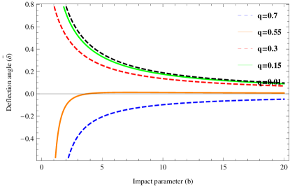
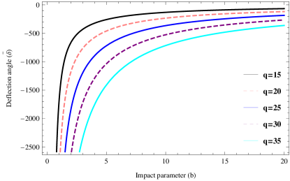
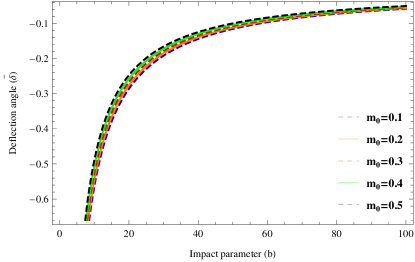
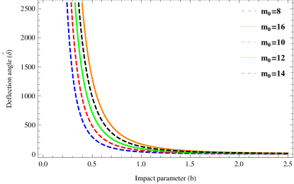
Figure 1: In 1 and 1, the behavior of deflection angle ($\tilde{\delta}$) with respect to impact parameter ($b$) for varying $q$ but fixed $m_{0}=1$. In 1 and 1, the behavior of $\tilde{\delta}$ with respect to $b$ for varying $m_{0}$ but fixed $q=1$. Here, $\Lambda^{\prime}=c=c_{1}=1$.

Here, from the plots 1 and 1, it is clear that the deflection angle decreases with the impact parameter for very small $q$ but remains positive. In contrast, for large $q$, the deflection angle increases with $b$ but takes negative values only. However, from figures 1 and 1, we see that the deflection angle increases with the impact parameter for small $m_{0}$ and remains negative valued. For larger black hole mass, the deflection angle is asymptotically decreasing function but remains positively valued.

4.2 Effect of charge ($q$) on deflection angle ($\tilde{\delta}$)

To study the effect of electric charge $q$ on deflection angle, we plot figure 2.

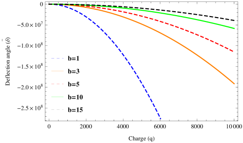
Figure 2: The behavior of deflection angle ($\tilde{\delta}$) with respect to charge $q$ by varying $b$. Here, $m=m_{0}=\Lambda^{\prime}=c=c_{1}=1$.

From the plot, we observe that the deflection angle is a decreasing function of $q$. The value of deflection angle becomes more negative when impact parameter increases.

4.3 Effect of mass parameter ($m$) on deflection angle ($\tilde{\delta}$)

To study the effect of the mass parameter ($m$) on deflection angle, we plot figure 3.

$\begin{array}[]{cccc}\begin{@subfigure}\includegraphics[width=216.81pt]{m1.eps}\end{@subfigure}\begin{@subfigure}\includegraphics[width=216.81pt]{m3.eps}\end{@subfigure}\end{array}$

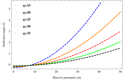
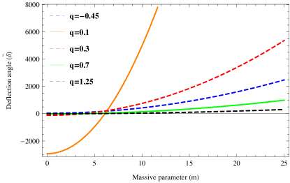
Figure 3: The behavior of $\tilde{\delta}$ with respect to $m$ by changing charge $q$. Here, $b=m_{0}=\Lambda^{\prime}=c=c_{1}=1$.

The plot tells that the deflection parameter is an increasing function of the mass parameter. There is a critical value for deflection angle that does not depend on the value of $q$. However, for the larger value of $q$, the deflection angle for massive black holes decreases. In 3, we see that for very small $q$, the deflection angle takes a negative value for small $m$.

4.4 Effect of cosmological constant ($\Lambda^{\prime}$) on deflection angle ($\tilde{\delta}$)

The impacts of cosmological constant ($\Lambda^{\prime}$) on deflection angle ($\tilde{\delta}$) are depicted in figure 4.

$\begin{array}[]{cccc}\begin{@subfigure}\includegraphics[width=216.81pt]{Lambda1.eps}\end{@subfigure}\begin{@subfigure}\includegraphics[width=216.81pt]{Lambda3.eps}\end{@subfigure}\end{array}$

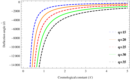
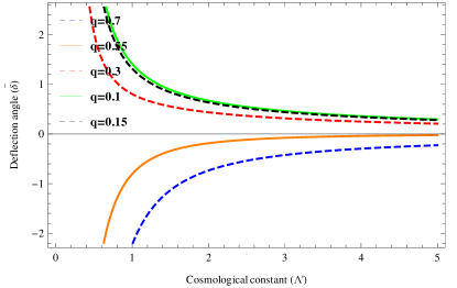
Figure 4: Plot of $\tilde{\delta}$ with respect to $\Lambda^{\prime}$ by changing $q$. Here, $b=m_{0}=m=c=c_{1}=1$.

From the figure 4 and 4, we see that deflection angle is both increasing and decreasing function with respect to $\Lambda^{\prime}$ according to different $q$. For large $q$, it is negative valued but increases with $q$. However, for very small values of $q$ it shows opposite character.

5 Gravitational lensing by linearly charged massive BTZ black hole in plasma medium

In this section, we study the gravitational lensing of linearly charged massive BTZ black hole filled with a cold non-magnetized plasma with the refractive index $n$. The refractive index satisfies the following relation [55]:

$$n^{2}(r)=1-\frac{\omega_{e}^{2}(r)}{\omega_{\infty}^{2}(r)}f(r),$$ (5.1)

where $\omega_{\infty}$ is the light ray frequency measured by a static viewer at infinity, while $\omega_{e}$ is the electron plasma frequency. The above refractive index simplifies to

$$n(r)=\sqrt{1-\frac{\omega_{e}^{2}}{\omega_{\infty}^{2}}(\Lambda^{\prime}r^{2}-m_{0}-2q^{2}\ln\left(\frac{r}{l}\right)+m^{2}cc_{1}r)}.$$ (5.2)

For the given black hole, described by static spherically symmetric metric surrounded by a plasma, the optical metric is given by

$$dt^{2}=g_{ij}^{opt}dx^{i}dx^{j}=n^{2}\left[\frac{dr^{2}}{f^{2}(r)}+\frac{r^{2}d\phi^{2}}{f(r)}\right].$$ (5.3)

The determinant of optical metric tensor $g_{ij}^{opt}$ is calculated as follows:

$$\sqrt{\det(g^{opt}_{ij})} = \frac{1}{{\Lambda^{\prime}}^{\frac{3}{2}}r^{2}}(1-\frac{\omega_{e}^{2}}{\omega_{\infty}^{2}}\Lambda^{\prime}r^{2})+\frac{m_{0}}{2{\Lambda^{\prime}}^{\frac{5}{2}}r^{4}}(3-\frac{\omega_{e}^{2}}{\omega_{\infty}^{2}}\Lambda^{\prime}r^{2})$$ (5.4)

$$+ \frac{q^{2}}{{\Lambda^{\prime}}^{\frac{5}{2}}r^{4}}\ln\left(\frac{r}{l}\right)(3-\frac{\omega_{e}^{2}}{\omega_{\infty}^{2}}\Lambda^{\prime}r^{2})-\frac{m^{2}cc_{1}}{2{\Lambda^{\prime}}^{\frac{5}{2}}r^{3}}(3-\frac{\omega_{e}^{2}}{\omega_{\infty}^{2}}\Lambda^{\prime}r^{2}).$$

Gaussian curvature in the form of curvature tensor can be calculated as

$$\mathcal{K} = \frac{R_{r\phi r\phi}\left(g^{opt}_{ij}\right)}{\det\left(g^{opt}_{ij}\right)},$$ (5.5)

$$= \frac{1}{\sqrt{\det\left(g^{opt}_{ij}\right)}}\left[\frac{\partial}{\partial\phi}\left(\frac{\sqrt{\det\left(g^{opt}_{ij}\right)}}{{g}_{rr}^{opt}}{\Gamma}_{rr}^{\phi}\right)-\frac{\partial}{\partial r}\left(\frac{\sqrt{\det\left(g^{opt}_{ij}\right)}}{{g}^{opt}_{rr}}{\Gamma}_{r\phi}^{\phi}\right)\right],$$

$$= \Lambda^{\prime}m_{0}(-1+\frac{\omega_{e}^{2}}{2\omega_{\infty}^{2}}\Lambda^{\prime}r^{2}-\frac{\omega_{e}^{4}}{\omega_{\infty}^{4}}\Lambda^{\prime}r^{2}+\frac{3\omega_{e}^{4}}{\omega_{\infty}^{4}}{\Lambda^{\prime}}^{2}r^{4})+\Lambda^{\prime}q^{2}(3+\frac{\omega_{e}^{2}}{\omega_{\infty}^{2}}\Lambda^{\prime}r^{2}+\frac{3\omega_{e}^{4}}{\omega_{\infty}^{4}}\Lambda^{\prime}r^{2})$$

$$- \frac{3\omega_{e}^{4}}{\omega_{\infty}^{4}}{\Lambda^{\prime}}^{2}r^{4}+\Lambda^{\prime}q^{2}\ln\left(\frac{r}{l}\right)(-2+\frac{2\omega_{e}^{2}}{\omega_{\infty}^{2}}\Lambda^{\prime}r^{2}+\frac{\omega_{e}^{2}}{\omega_{\infty}^{2}}r^{2}-\frac{2\omega_{e}^{4}}{2\omega_{\infty}^{4}}\Lambda^{\prime}r^{2})-\frac{q^{2}m_{0}}{r^{2}}$$

$$+ \frac{6q^{2}m^{2}cc_{1}}{r}\ln\left(\frac{r}{l}\right)+\frac{2q^{2}m^{2}cc_{1}}{r}+O(q^{4},m^{4},c^{2},c_{1}^{2}).$$

Now, to calculate the bending angle in the weak field limit of the light ray using the Gauss-Bonnet theorem and to compare it with non-plasma medium, we consider it at linear order only as

$$\tilde{\delta}=-\lim_{{\cal R}\rightarrow 0}\int_{0}^{\pi}\int_{\frac{b}{\sin\phi}}^{\cal R}\mathcal{K}dS.$$ (5.6)

Now, we calculate the quantity $\mathcal{K}dS$ as

$$\mathcal{K}dS = -\frac{(m_{0}-3q^{2})}{{\Lambda^{\prime}}^{\frac{1}{2}}r^{2}}+\frac{m_{0}^{2}}{2{\Lambda^{\prime}}^{\frac{1}{2}}r^{2}}\frac{\omega_{e}^{2}}{\omega_{\infty}^{2}}-\frac{m_{0}}{{\Lambda^{\prime}}^{\frac{3}{2}}r^{4}}\left(\frac{3m_{0}}{2}-8q^{2}\right)$$ (5.7)

$$- \frac{3m_{0}^{2}}{2{\Lambda^{\prime}}^{\frac{1}{2}}r^{2}}\frac{\omega_{e}^{4}}{\omega_{\infty}^{4}}+\frac{m^{2}cc_{1}}{2{\Lambda^{\prime}}^{\frac{3}{2}}r^{3}}(3m_{0}-5q^{2})+O(q^{4},m^{4},c^{2},c_{1}^{2}).$$

With the help of Eqs. (5.6) and (5.7), we obtain the deflection angle of linearly charged massive BTZ black hole in plasma medium as

$$\tilde{\delta} = \frac{2(m_{0}-3q^{2})}{{\Lambda^{\prime}}^{\frac{1}{2}}b}-\frac{m_{0}^{2}}{2{\Lambda^{\prime}}^{\frac{1}{2}}b}\frac{\omega_{e}^{2}}{\omega_{\infty}^{2}}+\frac{4m_{0}}{9{\Lambda^{\prime}}^{\frac{3}{2}}b^{3}}\left(\frac{3m_{0}}{2}-8q^{2}\right)$$ (5.8)

$$+ \frac{3m_{0}^{2}}{{\Lambda^{\prime}}^{\frac{1}{2}}b}\frac{\omega_{e}^{4}}{\omega_{\infty}^{4}}-\frac{m^{2}cc_{1}\pi}{8{\Lambda^{\prime}}^{\frac{3}{2}}b^{2}}(3m_{0}-5q^{2}).$$

Here, we see that, similar to the previous case, the deflection angle calculated for the plasma medium also depends on parameters like $q,b,m$, and $\Lambda^{\prime}$.

6 Graphical analysis for plasma medium

In this section, we analyse the behavior of deflection angle of charged massive black hole in plasma medium and its dependence on various parameters.

6.1 Effect of impact parameter ($b$) on deflection angle ($\tilde{\delta}$)

To study the behavior of deflection parameter and its dependence on impact parameter for varying $q$ and $m_{0}$, we plot figure 5.

$\begin{array}[]{cccc}\begin{@subfigure}\includegraphics[width=216.81pt]{b2.eps}\end{@subfigure}\begin{@subfigure}\includegraphics[width=216.81pt]{b3.eps}\end{@subfigure}\\ \begin{@subfigure}\includegraphics[width=216.81pt]{b22.eps}\end{@subfigure}\begin{@subfigure}\includegraphics[width=216.81pt]{b24.eps}\end{@subfigure}\end{array}$

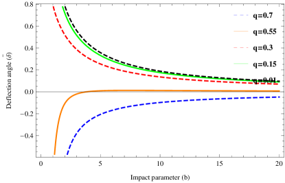
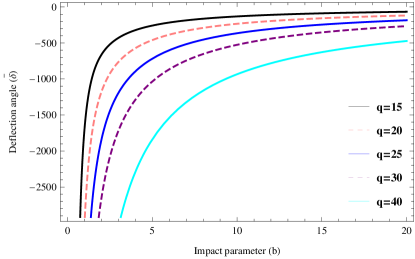
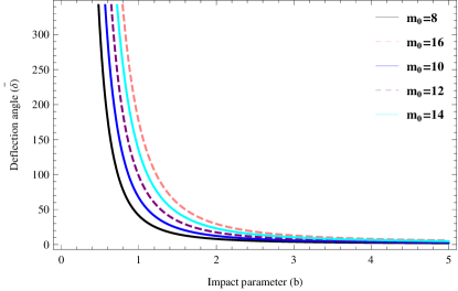
Figure 5: the behavior of deflection angle ($\tilde{\delta}$) with respect to impact parameter ($b$) for varying $q$ but fixed $m_{0}=1$ is depicted in 5 and 5. The behavior of $\tilde{\delta}$ with respect to $b$ for varying $m_{0}$ but fixed $q=1$ is depicted in 5 and 5. Here, $\Lambda^{\prime}=c=c_{1}=1$.

From the plots, we see that the deflection angle is an exponentially decreasing function of $b$ for large $m_{0}$ and very small $q$ but it takes always a positive value. However, the deflection angle is an exponentially increasing function of $b$ for very small $m_{0}$ and large $q$ but it takes always negative values. For large values of $b$, the deflection angle saturates.

6.2 Effect of charge ($q$) on deflection angle ($\tilde{\delta}$)

From the plot 6, we see that the deflection angle is a decreasing function of $q$ in a plasma medium and becomes more negative for smaller $b$.

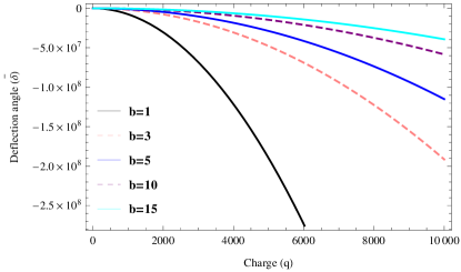
Figure 6: The behavior of $\tilde{\delta}$ with respect to $q$ by changing impact parameter $b$. Here, $b=m_{0}=\Lambda^{\prime}=c=c_{1}=1$.

6.3 Effect of mass parameter ($m$) on deflection angle ($\tilde{\delta}$)

The dependence of defection angle on mass parameter by varying charge $q$ is depicted in figure 7. The deflection angle is an increasing function of mass parameter $m$.

$\begin{array}[]{cccc}\begin{@subfigure}\includegraphics[width=216.81pt]{m2.eps}\end{@subfigure}\begin{@subfigure}\includegraphics[width=216.81pt]{m4.eps}\end{@subfigure}\end{array}$

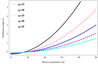
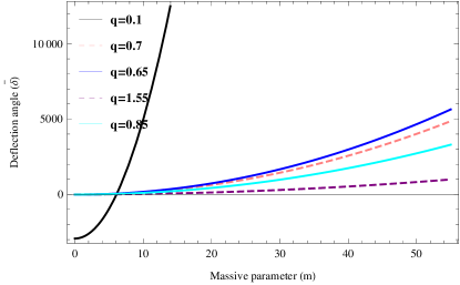
Figure 7: The behavior of $\tilde{\delta}$ with respect to $m$ by changing charge $q$. Here, $b=m_{0}=\Lambda^{\prime}=c=c_{1}=1$.

In plot 7, we see that, for smaller $q$ values, the deflection angle curve decreases sharply. From figure 7, for small $m$ and very small $q$, the deflection angle is negative valued.

6.4 Effect of cosmological constant ($\Lambda^{\prime}$) on deflection angle ($\tilde{\delta}$)

$\begin{array}[]{cccc}\begin{@subfigure}\includegraphics[width=216.81pt]{Lambda2.eps}\end{@subfigure}\begin{@subfigure}\includegraphics[width=216.81pt]{Lambda4.eps}\end{@subfigure}\end{array}$

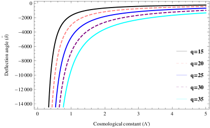
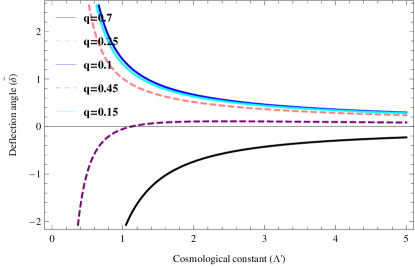
Figure 8: The behavior of $\tilde{\delta}$ with respect to $\Lambda^{\prime}$ with changing $q$. Here, $b=m_{0}=m=c=c_{1}=1$.

The behavior of deflection angle versus $\Lambda^{\prime}$ is depicted in figure 8. For large $q$, the deflection angle takes negative values but remains increasing function of $\Lambda^{\prime}$. However, for small $q$, the deflection angle is a positive but remains decreasing function of $\Lambda^{\prime}$.

7 Bound on greybody factor of linearly charged massive BTZ black hole

Greybody factors (transmission probability) in black hole physics is a quantity related to the quantum nature of a black hole which corrects the Planckian spectrum. The greybody factor describes the emissivity of the given black hole solution (non-perfect blackbody). Here, we determine the rigorous bound of the transmission probability of the linearly charged massive BTZ black hole. The general bounds of the greybody factor can be stated as [56]

$$T\geq\operatorname{sech}^{2}\left(\frac{1}{2\omega}\int_{-\infty}^{\infty}V(r)dr_{*}\right),$$ (7.1)

where $r_{*}$ denotes the tortoise coordinate and $\omega$ is the quasinormal mode frequency.

Event horizons (exterior and interior) can be calculated by vanishing metric function (i.e. $f(r)=0$). This gives

$$\Lambda^{\prime}r^{2}-m_{0}-2q^{2}\ln\left(\frac{r}{l}\right)+m^{2}cc_{1}r=0.$$ (7.2)

Considering $l=1$ and $\ln(r)=(r-1)$, the solution of the above equation can be written as

$$r_{\pm}=\frac{2q^{2}-m^{2}cc_{1}\pm\mathcal{G}}{2\Lambda^{\prime}},$$ (7.3)

where $\mathcal{G}=\sqrt{(m^{2}cc_{1}-2q^{2})^{2}-4\Lambda^{\prime}(2q^{2}-m_{0})}$.

Now, we analyze the Regge–Wheeler equation for angular momentum $l$ and derive rigorous bounds on the greybody factors. Let us define the Regge–Wheeler equation as

$$\left(\frac{d^{2}}{dr_{*}^{2}}+\omega^{2}-V(r)\right)\psi=0,$$ (7.4)

where

$$dr_{*}=\frac{1}{f(r)}dr,$$ (7.5)

and potential $V(r)$ in $3D$ is given as

$$V(r)=-\frac{1}{4}\frac{f^{2}(r)}{r^{2}}+\frac{1}{2}\frac{f(r)f^{\prime}(r)}{r}+l^{2}\frac{f(r)}{r^{2}}.$$ (7.6)

In order to discuss bound value of transmission probability, we first write bound in the expression (7.1) with the help of (7.5) as

$$T\geq\operatorname{sech}^{2}\left(\frac{1}{2\omega}\int_{r_{+}}^{\infty}\frac{V(r)dr}{f(r)}\right).$$ (7.7)

The lower bound value of transmission probability thus leads to

$$T\geq\operatorname{sech}^{2}\left[\frac{1}{2\omega}\int_{r_{+}}^{\infty}\left(-\frac{1}{4}\frac{f(r)}{r^{2}}+\frac{(1)}{2}\frac{f^{\prime}(r)}{r}+\frac{l^{2}}{r^{2}}\right)dr\right].$$ (7.8)

For the given metric function, mentioned in (7.2), the above simplifies to

$$T \geq \operatorname{sech}^{2}\left[\frac{1}{2\omega}\left\{\frac{1}{4}(\Lambda^{\prime}r_{+}+\frac{m_{0}}{r_{+}}+\frac{2q^{2}}{r_{+}}(\ln(\frac{r_{+}}{l})+1)+m^{2}cc_{1}\ln(r_{+})\right.\right.$$ (7.9)

$$+ \left.\left.\frac{1}{2}(-2\Lambda^{\prime}r_{+}-\frac{2q^{2}}{r_{+}}-m^{2}cc_{1}ln(r_{+}))+\frac{l^{2}}{r_{+}}\right\}\right].$$

Plugging the value of $r_{+}$ from equation (7.3), the bound on the greybody factor changes to

$$T \geq \operatorname{sech}^{2}\left[\frac{1}{2\omega}\left\{\frac{3}{8}(m^{2}cc_{1}-2q^{2}-\mathcal{G})+\frac{m_{0}\Lambda^{\prime}}{2(2q^{2}-m^{2}cc_{1}+\mathcal{G})}\right.\right.$$ (7.10)

$$+ \left.\left.\frac{\Lambda^{\prime}q^{2}}{2q^{2}-m^{2}cc_{1}+\mathcal{G}}\ln\left(\frac{2q^{2}-m^{2}cc_{1}+\mathcal{G}}{2\Lambda^{\prime}l}\right)-\frac{1}{4}m^{2}cc_{1}\ln\left(\frac{2q^{2}-m^{2}cc_{1}+\mathcal{G}}{2\Lambda^{\prime}}\right)\right.\right.$$

$$+ \left.\left.\frac{\Lambda^{\prime}(2l^{2}-q^{2})}{2q^{2}-m^{2}cc_{1}+\mathcal{G}}\right\}\right].$$

Special Cases:

• Case I: If massive BTZ black hole has no electric charge (i.e. $q=0$), then the bound on the greybody factor becomes

  $$T \geq \operatorname{sech}^{2}\left[\frac{1}{2\omega}\left\{\frac{3}{8}(m^{2}cc_{1}-\mathcal{G})+\frac{m_{0}\Lambda^{\prime}}{2(\mathcal{G}-m^{2}cc_{1})}-\frac{1}{4}m^{2}cc_{1}\ln(\frac{\mathcal{G}-m^{2}cc_{1}}{2\Lambda^{\prime}})\right.\right.$$ (7.11)

  $$+ \left.\left.\frac{2\Lambda^{\prime}l^{2}}{(\mathcal{G}-m^{2}cc_{1})}\right\}\right].$$

• Case II: In the massless limit ($m=0$), the bound on the greybody factor takes the following form:

  $$T \geq \operatorname{sech}^{2}\left[\frac{1}{2\omega}\left\{-\frac{3}{8}(2q^{2}+\mathcal{G})+\frac{m_{0}\Lambda^{\prime}}{2(2q^{2}+\mathcal{G})}+\frac{\Lambda^{\prime}q^{2}}{(2q^{2}+\mathcal{G})}\ln\left(\frac{2q^{2}+\mathcal{G}}{2\Lambda^{\prime}l}\right)\right.\right.$$ (7.12)

  $$+ \left.\left.\frac{\Lambda^{\prime}(2l^{2}-q^{2})}{(2q^{2}+\mathcal{G})}\right\}\right].$$

8 Comparative analysis of greybody factor

The behavior of potential is depicted in figure 9 for different values of $q$. Here, we see that, for very small $q$, potential is negative which describes a bound system.

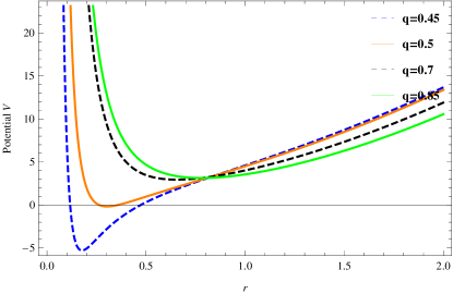
Figure 9: Potential ($V(r)$) versus $r$ for varying $q$ and for angular momentum ($l$) =1. Here, $\Lambda^{\prime}=m_{0}=m=c=c_{1}=l=1$.

The behavior of potential is depicted in figure 10 for different values of $m$.

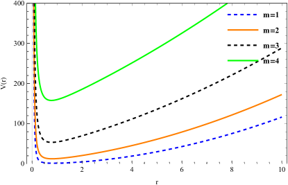
Figure 10: Potential ($V(r)$) versus $r$ for varying $m$ and for angular momentum ($l$) =1. Here, $\Lambda^{\prime}=m_{0}=q=c=c_{1}=l=1$.

The calculated bound with respect to $\omega$ is depicted in figure 11 for both small and large values of $q$. We see that the bound increases sharply and then saturates after certain value of $\omega$.

$\begin{array}[]{cccc}\begin{@subfigure}\includegraphics[width=216.81pt]{T1.eps}\end{@subfigure}\begin{@subfigure}\includegraphics[width=216.81pt]{T2.eps}\end{@subfigure}\end{array}$

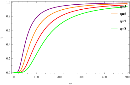
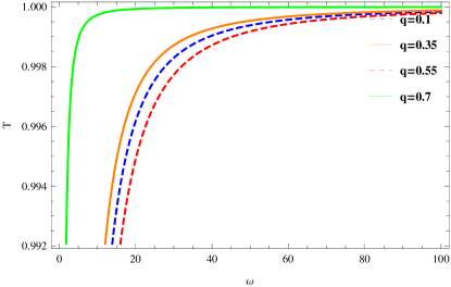
Figure 11: Plots for greybody factor lower bound with respect to $\omega$.

$\begin{array}[]{cccc}\includegraphics[width=216.81pt]{T03.eps}\end{array}$

Figure 12: Plots for greybody factor lower bound with respect to $\omega$ for changing $m$ but fixed angular momentum $l=1$. Here, $\Lambda^{\prime}=q=m_{0}=c=c_{1}=l=1$.

From figure 11, we see that the value of bound decreases along with larger values of charge (in the large domain). In figure 11, we observe that the value of bound increases along with larger values of charge (in the small domain).

9 Shadow of charged massive BTZ black hole

In order to study the null geodesics for linearly charged massive BTZ black hole, we use Hamilton-Jacobi method. To obtain the shadow of this black hole, we calculate the celestial coordinates of the unstable null orbits. The motion of the particle on the linearly charged massive BTZ black hole is described by the following Lagrangian:

$$\mathcal{L}=\frac{1}{2}g_{\mu\nu}u^{\mu}u^{\nu}.$$ (9.1)

Here, $u^{\mu}(=\frac{dx^{\mu}}{d\lambda})$ represents the four velocity of particle with affine parameter $\lambda$ along the geodesics. Since, the metric does not depend on the coordinate $t$ and $\phi$, so we get two constants of motion corresponding to these, namely, energy $E$ and angular momentum $h$ as follows

$$E=p_{t}=\frac{d\mathcal{L}}{d\dot{t}}=g_{\phi t}\dot{\phi}+g_{tt}\dot{t}\;\ \ \mbox{and}\;\ \ h=-p_{\phi}=-\frac{d\mathcal{L}}{dt\dot{\phi}}=-g_{\phi\phi}\dot{\phi}-g_{\phi t}\dot{t}.$$ (9.2)

The derivatives of $t$ and $\phi$ with affine parameter $\lambda$ is derives as

$$\frac{dt}{d\lambda}=\frac{E}{f(r)},\ \ \ \ \ \frac{d\phi}{d\lambda}=\frac{h}{r^{2}\sin^{2}\theta}.$$ (9.3)

The other geodesics equations can be estimated with the help of following relativistic Hamilton-Jacobi equation:

$$\frac{dS}{d\lambda}=\frac{1}{2}g^{\mu\nu}\frac{dS}{dx^{\mu}}\frac{dS}{dx^{\nu}},$$ (9.4)

where $S$ refers to Jacobi action. In order to calculate the Hamilton-Jacobi equation, we consider an ansatz of the form [57]

$$S=\frac{1}{2}m_{\star}^{2}\lambda-Et+h\phi+S_{r}(r)+S_{\theta}(\theta)$$ (9.5)

where $m_{\star}$ is the mass of the test particle, $S_{r}(r)$ and $S_{\theta}(\theta)$ correspond to the functions of $r$ and $\theta$. In the charged massive BTZ black hole spacetime, the Hamilton-Jacobi equation leads to

$$\frac{1}{2}g^{tt}\frac{\partial{S}}{\partial{x^{t}}}\frac{\partial{S}}{\partial{x^{t}}}+g^{\phi t}\frac{\partial{S}}{\partial{x^{t}}}\frac{\partial{S}}{\partial{x^{\phi}}}+\frac{1}{2}g^{rr}\frac{\partial{S}}{\partial{x^{r}}}\frac{\partial{S}}{\partial{x^{r}}}+\frac{1}{2}g^{\theta\theta}\frac{\partial{S}}{\partial{x^{\theta}}}\frac{\partial{S}}{\partial{x^{\theta}}}+\frac{1}{2}g^{\phi\phi}\frac{\partial{S}}{\partial{x^{\phi}}}\frac{\partial{S}}{\partial{x^{\phi}}}=-\dot{S}.$$ (9.6)

Considering method of separation of variables, the solutions of $S_{r}$ and $S_{\theta}$ for null geodesic for massless particle (photon) can be given, respectively, as [58]

$$\Sigma\frac{\partial{S_{r}}}{\partial{r}} = \pm\sqrt{\mathcal{R}(r)},$$ (9.7)

$$\Sigma\frac{\partial{S_{\theta}}}{\partial{\theta}} = \pm\sqrt{\Theta(\theta)},$$ (9.8)

where $\mathcal{R}(r)=r^{4}E^{2}-(h^{2}+\mathbb{K})r^{2}f(r)$ and $\Theta(\theta)=\mathbb{K}-h^{2}\cot^{2}\theta$ with the Carter constant $\mathbb{K}$. For a far observer, the photon comes to charged massive BTZ black hole near the equatorial plane and the unstable circular orbits follow: $\mathcal{R}(r)|_{r=r_{p}}=\mathcal{R}^{\prime}(r)|_{r=r_{p}}=0$. Here, “prime(^′)” denotes derivative with respect of $r$ and $r_{p}$ is the radius of the unstable circular null orbit.

Now, we introduce two dimensionless impact parameters $\xi$ and $\eta$ defined in terms of $h$, $E$ and $\mathbb{K}$, as

$$\xi=\frac{h}{E}\ \ \mbox{and}\ \ \eta=\frac{\mathbb{K}}{E^{2}}.$$ (9.9)

In terms of these dimensionless impact parameters, the solution $\mathcal{R}(r)$ can be expressed as

$$\mathcal{R}(r)=r^{4}E^{2}-r^{2}E^{2}(\xi^{2}+\eta)f(r).$$ (9.10)

Here, we note that $\mathcal{R}(r)$ acts as an effective potential for the photon moving along $r$ direction. With the help of relations (9.7) and (9.10), the equation for $S_{r}$ can be written as

$$\left(\frac{\partial{S_{r}}}{\partial{r}}\right)^{2}+V_{eff}=0,$$ (9.11)

where the effective potential $V_{eff}$ is given by

$$V_{eff}=\frac{1}{\Sigma^{2}}\left[r^{2}{f(r)}{}E^{2}(\xi^{2}+\eta)-r^{4}E^{2}\right].$$ (9.12)

Two conditions that unstable circular orbit follow, in terms of effective potential, turn to

$$\left.V_{eff}(r)\right|_{r=r_{p}}=0,\ \ \ \ \left.\frac{\partial{V_{eff}(r)}}{\partial{r}}\right|_{r=r_{p}}=0.$$ (9.13)

For the give potential (9.12), the first condition $V_{eff}(r)|_{r=r_{p}}=0$ gives

$$\eta+\xi^{2}=\frac{r_{p}^{2}}{f(r_{p})}.$$ (9.14)

The second boundary condition $\left.\frac{\partial{V_{eff}(r)}}{\partial{r}}\right|_{r=r_{p}}=0$, together with the first one, leads to

$$r_{p}f^{\prime}(r_{p})=2f(r_{p}).$$ (9.15)

We can estimate the shadow size from Eq. (9.14) upon substituting the photon sphere radius $r_{p}$. Using Eq. (9.15) and metric function of BTZ black hole, $r_{p}$ is calculated as

$$r_{p}=\frac{6q^{2}-2m_{0}}{4q^{2}-m^{2}cc_{1}}.$$ (9.16)

The celestial coordinates of the distant observer measured in the directions perpendicular ($X$) and parallel ($Y$) to the projected rotation axis describe the apparent angular distances of the image on the (celestial) sphere. For the present case, the celestial coordinates are given by

$$X=\lim_{r_{p}\to\infty}\left(\left.-r^{2}_{p}\sin\theta_{0}\frac{d\phi}{dr}\right|_{(r_{p},\theta_{0})}\right),$$ (9.17)

and

$$Y=\lim_{r_{p}\to\infty}\left(\left.r^{2}_{p}\frac{d\theta}{dr}\right|_{(r_{p},\theta_{0})}\right),$$ (9.18)

where $\theta_{0}$ is the angular coordinate of the distant observer. For the null geodesic, this leads to

$$X=-\frac{\xi}{\sin\theta},$$ (9.19)

$$Y=\pm\sqrt{\eta-\xi^{2}\cot^{2}\theta},$$ (9.20)

which, in fact, relate the celestial coordinates and impact parameters. In case when the observer is on the equatorial plane of the black hole (i.e, $\theta_{0}=\frac{\pi}{2}$), the celestial coordinates take the values:

$$X=-\xi,$$ (9.21)

$$Y=\pm\sqrt{\eta}.$$ (9.22)

Therefore, the radius of the shadow can be given by

$$R_{s}=\sqrt{X^{2}+Y^{2}}=\sqrt{\eta+\xi^{2}}=\sqrt{\frac{r^{2}_{p}}{f(r_{p})}}.$$ (9.23)

Now, we demonstrate the computed values of the shadow radius $R_{s}$ for different values of cosmological constant ($\Lambda^{\prime}$) of the charged BTZ black hole in table 2. Table 2 shows the values of the shadow radius ($R_{s}$) for different values of charge ($q$).

$q$	$r_{p}$	$\Lambda^{\prime}$	$R^{2}_{s}$
		0.45	3.80816
		0.55	2.75791
1	1.333	0.67	2.07214
		0.75	1.77748
		0.84	1.4233
		4.00	3.85718
		4.15	2.44345
3	1.48571	4.25	1.9365
		4.35	1.64134
		4.45	1.40993

Table 1: Radius of the black hole shadow $R_{s}$ for varying $\Lambda^{\prime}$ with fixed $q$ and $r_{p}$.

$\Lambda^{\prime}$	$q$	$r_{p}$	$R^{2}_{s}$
	1	1.333	0.262289
	1.5	1.4375	0.306845
4	2	1.4667	0.403015
	2.5	1.47917	0.675016
	2.8	1.48353	1.29066
	1	1.333	0.17204
	1.5	1.4375	0.190151
6	2	1.4667	0.223154
	2.5	1.47917	0.287237
	2.8	1.48353	0.360386

Table 2: Radius of the black hole shadow $R_{s}$ for varying charge $q$ with fixed $\Lambda^{\prime}$.

The black hole shadows for different values of cosmological constant, charge and mass parameter are depicted in Figs. 13, 14 and 15, respectively. Here, we observe that the shadow radius decreases with increase in cosmological constant and mass parameter. However, the shadow radius increases with increase in photon radius and charge. In figure 16 and 17, we see that shadow radius is a decreasing function of cosmological constant and mass parameter, however, it is an increasing function of charge.

$\begin{array}[]{cccc}\begin{@subfigure}\includegraphics[width=216.81pt]{s1.eps}\end{@subfigure}\begin{@subfigure}\includegraphics[width=216.81pt]{s2.eps}\end{@subfigure}\end{array}$

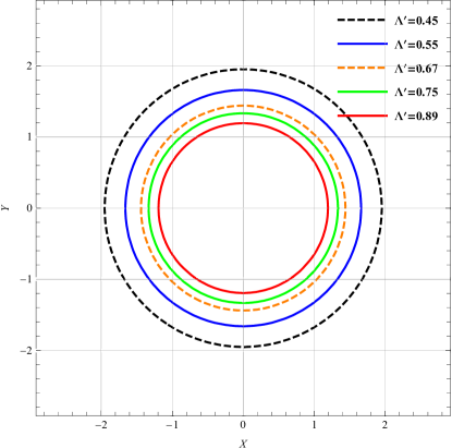
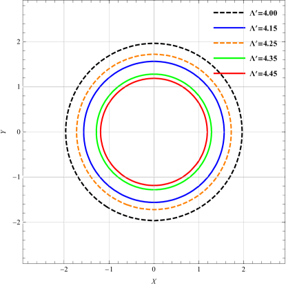
Figure 13: Black hole shadow in the celestial plane for different values of cosmological constant $\Lambda^{\prime}$. In (a), charge $q=1$ and photon radius $r_{p}=1.333$. In (b) charge $q=3$ and photon radius $r_{p}=1.48571$. Here $m_{0}=m=c=c_{1}=1$.

$\begin{array}[]{cccc}\begin{@subfigure}\includegraphics[width=216.81pt]{s3.eps}\end{@subfigure}\begin{@subfigure}\includegraphics[width=216.81pt]{s4.eps}\end{@subfigure}\end{array}$

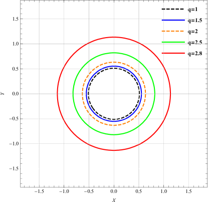
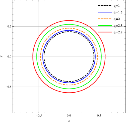
Figure 14: Black hole shadow in the celestial plane for different values of charge $q$. In (a), $\Lambda^{\prime}=4$. In (b), $\Lambda^{\prime}=6$. Here $m_{0}=m=c=c_{1}=1$.

$\begin{array}[]{cccc}\begin{@subfigure}\includegraphics[width=216.81pt]{m01.eps}\end{@subfigure}\begin{@subfigure}\includegraphics[width=216.81pt]{m02.eps}\end{@subfigure}\end{array}$

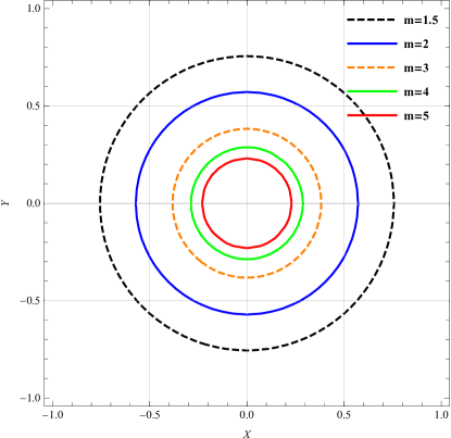
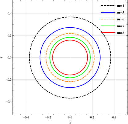
Figure 15: Black hole shadow in the celestial plane for different values of massive parameter $m$. In (a), charge $q=1$ and photon radius $r_{p}=1.333$. In (b) charge $q=3$ and photon radius $r_{p}=1.48571$. Here, $m_{0}=\Lambda^{\prime}=c=l=c_{1}=1$.

$\begin{array}[]{cccc}\begin{@subfigure}\includegraphics[width=216.81pt]{s5.eps}\end{@subfigure}\begin{@subfigure}\includegraphics[width=216.81pt]{s6.eps}\end{@subfigure}\end{array}$

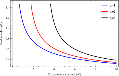
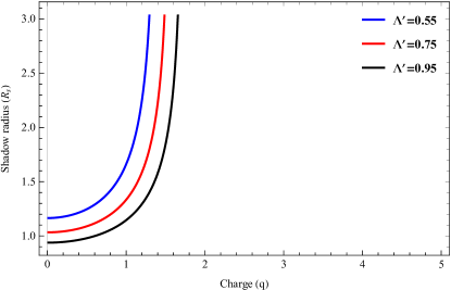
Figure 16: In (a): variation of the radius of the black hole shadow $R_{s}$ with cosmological constant $\Lambda^{\prime}$ for varying charge $q$. In (b): variation of the radius of the black hole shadow $R_{s}$ with charge $q$ for varying cosmological constant $\Lambda^{\prime}$.

$\begin{array}[]{cccc}\begin{@subfigure}\includegraphics[width=216.81pt]{Rs01.eps}\end{@subfigure}\begin{@subfigure}\includegraphics[width=216.81pt]{Rs02.eps}\end{@subfigure}\end{array}$

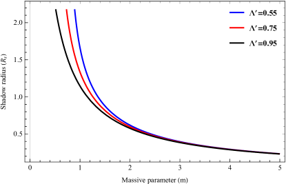
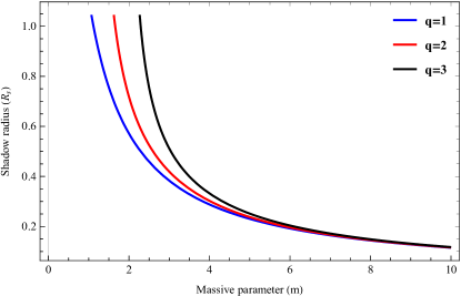
Figure 17: In (a): variation of the radius of the black hole shadow $R_{s}$ with massive parameter $m$ for varying cosmological constant $\Lambda^{\prime}$. Here, $q=m_{0}=c=l=c_{1}=1$. In (b): variation of the radius of the black hole shadow $R_{s}$ with massive parameter $m$ for varying charge $q$. Here, $\Lambda^{\prime}=m_{0}=c=l=c_{1}$. Both plots are for photon sphere radius $r_{p}=1.333$.

10 Summary and final remarks

The existence of very compact objects (like black holes) is now well-established through astrophysical observations. In the locality of black holes, light ray travels through very strong gravitational fields. Black holes in a very unique sense provide an opportunity to study gravitational lensing beyond the first order weak deflection limit (which governs most gravitational lensing). However, the study of this new approach requires very strong technical abilities.

In this work, we have considered a charged black hole solution in massive gravity and with the help of null geodesics we have calculated optical metric. This optical metric induces Gaussian optical curvature in weak gravitational lensing. Applying the Gauss-Bonnet theorem, we have calculated the deflection angle from the Gaussian curvature of the optical metric for the black hole in a non-plasma medium. Here, we have found that the deflection angle of charged massive BTZ black hole depends on the various parameters like impact parameter, charge, the mass parameter, graviton mass and cosmological constant. To check the dependency of the deflection parameter on these parameters, we have done a graphical analysis. The graphs declared that the deflection angle decreases and increases with the impact parameter for very small and large values of charge, receptively. However, the deflection angle increases and decreases along with the impact parameter for small and large masses, respectively. We also found that the deflection angle is a decreasing and increasing function of charge and mass of black hole, respectively.

Within the context of gravitational lensing, we also computed Gaussian optical curvature for the charged massive BTZ black hole filled with a cold spherically symmetric non-magnetized plasma. The Gauss-Bonnet theorem can be used to study the light rays in a plasma medium by following a correlation between timelike geodesics pursued by light rays in a plasma medium and spatial geodesics in an associated optical geometry. The resulting deflection angle in the plasma medium has additional terms due to the refractive index of the plasma medium. We have provided the graphical analyses for the plasma medium case also, which reflects the dependencies of the deflection angle on various parameters. The rigorous analytic bounds on the greybody factors of the linearly charged massive BTZ black hole are also derived. From the potential and bound on greybody factor graphs, we observed that the system is not bound for a large value of charge and the bound increases sharply and then saturates after a certain value of quasinormal mode frequency. Finally, we studied the shadow of charged massive BTZ black holes for a distant observer. The effects of charge and cosmological constant on the shadow radius are also analyzed. In this connection, we have found that the shadow radius decreases with increase in cosmological constant. In contrast, the shadow radius increases with increase in photon radius and charge.

The present analysis may be useful to probe the signature of massive gravity in the shadow of black holes which in turn may be a candidate for dark matter. The present analysis may be helpful in estimating correct value of cosmological constant as a possible source of dark energy present in the universe. It will be interesting to generalize these results to the other gravity models such as Lee-Wick gravity and $f(R)$ gravity.

Data Availability Statement

Data sharing not applicable to this article as no datasets were generated or analysed during the current study.

References

- [1] M. Banados, C. Teitelboim and J. Zanelli, Phys. Rev. Lett. 69 (1992) 1849.
- [2] E. Witten, arXiv:0706.3359.
- [3] E. Witten, Adv. Theor. Math. Phys. 2 (1998) 505.
- [4] A. Larranaga, Commun. Theor. Phys. 50 (2008) 1341.
- [5] M. Cadoni and C. Monni, Phys. Rev. D 80 (2009) 024034.
- [6] T. Sarkar, G. Sengupta and B. Nath Tiwari, JHEP 11 (2006) 015.
- [7] R. Emparan, G. T. Horowitz and R. C. Myers, JHEP 01 (2000) 021.
- [8] M. R. Setare, Eur. Phys. J. C 49 (2007) 865.
- [9] S. Carlip, Class. Quantum Gravit. 22 (2005) R85.
- [10] E. Frodden, M. Geiller, K. Noui and A. Perez, JHEP 05 (2013) 139.
- [11] A. de la Fuente and R. Sundrum, JHEP 09 (2014) 073.
- [12] M. Cardenas, O. Fuentealba and C. Martinez, Phys. Rev. D 90 (2014) 124072.
- [13] S. H. Hendi, B. Eslam Panah, R. Saffari, Int. J. Mod. Phys. D 23 (2014) 1450088.
- [14] P. Valtancoli, Annals Phys. 369 (2016) 161.
- [15] B. Gwak and B. H. Lee, Phys.Lett. B 755 (2016) 324.
- [16] S. H. Hendi, B. Eslam Panah and S. Panahiyan, JHEP 05 (2016) 029.
- [17] E. Maghsoodi, H. Hassanabadi and W. S. Chung, PTEP 2019, 083E03 (2019).
- [18] K. Jusufi, H. Hassanabadi,P. Sedaghatnia, et al, Eur. Phys. J. Plus 137, 1147 (2022).
- [19] H. Chen, B. C. Lütfüoğlu, H. Hassanabadi and Z.-Wen Long, 827 (2022) 136994.
- [20] N. Farahani, et al., Eur. Phys. J. C 80, 696 (2020).
- [21] H. Hassanabadi, et al., Eur. Phys. J. C 79, 936 (2019).
- [22] E. Maghsoodi, et al., Physics of the Dark Universe 28 (2020) 100559.
- [23] H. Hassanabadi, E. Maghsoodi and W. S. Chung, Eur. Phys. J. C 79, 358 (2019).
- [24] L. Hui, J.P. Ostriker, S. Tremaine, E. Witten, Phys. Rev. D95, 043541 (2017).
- [25] A. Arvanitaki, S. Dimopoulos, S. Dubovsky, N. Kaloper and J. March-Russell, Phys. Rev. D81, 123530 (2010).
- [26] A. Lewis and A. Challinor, Physics Reports 429, 1 (2006).
- [27] G. W. Gibbons and M. C. Werner, Class. Quant. Grav. 25, 235009 (2008).
- [28] V. Acquaviva, C. Baccigalupi and F. Perrotta, Proceedings of the International Astronomical Union, 2004 (2004) 123.
- [29] A. Övgün, I. Sakalli and J. Saavedra, Annals of Physics 411 (2019) 167978.
- [30] D. N. Page, Phys. Rev. D 13 (1976) 198.
- [31] P. Boonserm and M. Visser, Phys. Rev. D 78, 101502 (2008).
- [32] D. C. Dai and D. Stojkovic, JHEP 08 (2010) 016.
- [33] S. Fernando, Gen. Rel. Grav. 37 (2005) 461.
- [34] R. Mistry, S. Upadhyay, A. F. Ali and M. Faizal, Nucl. Phys. B 923 (2017) 378.
- [35] P. Kanti and J. March-Russell, Phys. Rev. D 66 (2002) 024023.
- [36] P. Kanti, J. Grain and A. Barrau, Phys. Rev. D 71 (2005) 104002.
- [37] R. A. Konoplya and A. F. Zinhailo, Phys. Lett. B 810, 135793 (2020).
- [38] W. Javed, M. Aqib, A. Övgün, Phys. Lett. B 829, 137114 (2022).
- [39] P. Gonzalez, C. Campuzano, E. Rojas and J. Saavedra, JHEP 1006, 103 (2010).
- [40] I. Sakalli and S. Kanzi, Turk. J. Phys. 46 (2022) 51.
- [41] T. Harmark, J. Natario and R. Schiappa, Adv. Theor. Math. Phys. 14 (2010) 727.
- [42] I. Sakalli, Phys. Rev. D 94, 084040 (2016).
- [43] S. Kanzi, S. H. Mazharimousavi and I. Sakalli, Annals of Physics 422 (2020) 168301.
- [44] P. Boonserm, C. H. Chen, T. Ngampitipan and P. Wongjun, Phys. Rev. D 104 (2021) 084054.
- [45] H. Gürsel and I. Sakalli, Eur. Phys. J. C 80, 234 (2020).
- [46] A. Al-Badawi, S. Kanzi and I. Sakalli, Eur. Phys. J. Plus 137 (2022) 94.
- [47] S. Kanzi, I. Sakalli, Nucl. Phys. B 946, (2019) 114703.
- [48] H. Falcke, F. Melia, and E. Agol, ApJL 528, L13 (2000).
- [49] J. L. Synge, MNRAS, 131, 463 (1966).
- [50] A. Övgün and I. Sakalli, Class. Quantum Grav. 37, 225003 (2020).
- [51] A. Övgün and I. Sakalli, J. Saavedra, JCAP 10 (2018) 041.
- [52] S. H. Hendi, B. Eslam Panah and S. Panahiyan, Phys. Lett. B 769 (2017) 191.
- [53] E. F. Eiroa, G. E. Romero and D. F. Torres, Phys. Rev. D 66, 024010 (2002).
- [54] J. Ahmed and K. Saifullah, Eur. Phys. J. C 78 (2018) 316.
- [55] V. Perlick, O. Yu. Tsupko and G. S. Bisnovatyi-Kogan, Phys. Rev. D 92(10), 104031 (2015).
- [56] M. Visser, Phys. Rev. A 59 (1999) 427.
-
[57]
S. Chandrasekhar: The Mathematical Theory of Black Holes. Oxford University Press, Oxford (1998).
- [58] T. Johannsen, Astrophys. J. 777, 170 (2013).