Entanglement Entropy of Large-N Theories

Abstract

A large class of strongly correlated quantum systems can be described in certain large-N limits by quadratic in field actions along with self-consistency equations that determine the two-point functions. We use the replica approach and the notion of shifted Matsubara frequency to compute von Neumann and Rényi entanglement entropies for generic bi-partitioning of such systems. Remarkably, the von Neumann entropy can be computed from equilibrium spectral functions w/o partitioning, while the Rényi entropy requires re-calculating the spectrum in the interacting case. We demonstrate the flexibility of the method by applying it to examples of a two-site problem in presence of decoherence, and various coupled Sachdev-Ye-Kitaev models.

Entanglement is one of the central concepts of quantum mechanics and a notion based on which many of the modern physical phenomena are understood. The entanglement between the degrees of freedom in a region of space A and the rest of the system $\bar{\rm A}$, is fully characterized by the so-called entanglement spectrum (ES), i.e. eigenvalues of the reduced density matrix $\rho_{A}={\rm Tr}_{\bar{A}}[\rho]$, or equivalently their various moments. Among different measures of the entanglement, Rényi and von Neumann entanglement entropies (EEs)

$$S^{{\rm R}_{M}}_{A}\equiv\frac{1}{1-M}\log{\rm Tr}\left[\rho_{A}^{M}\right],\quad S^{\rm vN}_{A}\equiv-{\rm Tr}\left[\rho_{A}\log\rho_{A}\right],$$ (1)

are frequently used, where the latter can also be extracted from the limit $S^{\rm vN}_{A}=\lim_{M\to 1^{+}}S^{{\rm R}_{M}}_{A}$.

It is known that for pure states, EE of typical states depends on the sizes of the Hilbert spaces [1, 2]. However, the EE of the ground state scales with the spatial extents of regions. Intuitively, EE counts the number of entangled states; for gapped systems with short-range correlation an ‘area law’ and for gapless systems with long-range correlation, a ‘volume law’ is expected [3, 4, 5].

Two important applications are noteworthy; for 1+1 dimensional gapless systems, EE is the natural probe of the central charge of the underlying conformal field theory (CFT) [6]. In 2+1 dimensional gapped systems with perimeter $L_{A}$, the entropy has the form $S_{A}^{\rm vN}=\alpha L_{A}-\gamma$ [7], where $\gamma$ is a signature of topological order and can be extracted by eliminating the extensive part [8, 9].

Moreover, according to eigenstate thermalization hypothesis (ETH) [10, 11, 12], the reduced density matrix of a chaotic system in a pure state has the Boltzmann form $\rho_{A}\sim e^{-H_{A}/T_{\rm eff}}$ where $H_{A}$ is the Hamiltonian of detached A and temperature $T_{\rm eff}$ depends on the state’s energy. A somewhat unexpected example is the Laughlin state, whose ES contains the spectrum of gapless edge states that would exist if A and $\bar{\rm A}$ were detached [13], as if due to topology and despite the gap, $\rho_{A}$ shares the same spectrum with $H_{A}$. Similar physics has been seen in other topological systems [14, 15], and understood in terms of relevant coupling of edge states across A-$\bar{\rm A}$ border [16].

There are also connections to holography [17, 18]. According to Ryu-Takayanagi conjecture, the EE of CFT_d+1 is given geometrically $S_{A}^{\rm vN}\propto{\cal A}_{A}$ by the extremal area ${\cal A}_{A}$ of the minimal space-like surface anchored to $A$ region and extending in the AdS_d+2 bulk. As external parameters are varied, ${\cal A}_{A}$ may switch from isolated surfaces to a joint surface, interpreted as the formation of a wormhole. Hence, certain transitions in EE are holographically topological.

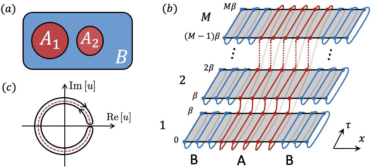
Figure 1: (a) General bi-partite setting considered in this paper. A and B sections do not need to be simply connected. (b) The replica method for computing Rényi entropy. The boundary condition in the imaginary time direction for A and B sections, represented by the red/blue lines, are different. (c) The contour integral used to define von Neumann EE in the fermionic case. Bosonic case is the vertical mirror of this.

Despite its prevalence and important applications, the class of problems where EE can be computed are limited to non-interacting problems [19, 20, 21], 2D CFTs [6, 22, 23], a number of integrable models [24, 25, 26], as well as systems amenable to quantum Monte Carlo [27, 28], exact diagonalization [29] or density matrix renormalization. Here, we extend this list to problems which can be described by quadratic actions, e.g. models studied with static mean-field [30, 31] and dynamical large-N techniques. The latter includes Sachdev-Ye-Kitaev (SYK) models [32] as well as various Kondo systems [33, 34, 35, 36, 37, 38, 39, 40, 41, 42, 43] and large-N theories of strange metals [44, 45]. To the best of our knowledge such a versatile technique was until now not available.

Previous attempts at calculating EE of these systems [46, 47, 48, 49, 50] have been mostly limited to 2^nd Rényi entropy and restricted to SYK model, which thanks to its exact solvability and maximally chaotic behavior [32], have attracted considerable interest. Thermalization of SYK and coupled-SYK models [51, 52, 53, 54, 55, 56], have been studied due to their holographic equivalence to blackholes, in certain regimes connected by traversable wormholes [52, 53].

In this paper, we develop a formalism to compute EE in larger-N theories and demonstrate its applicability to study EE in free-fermions and coupled-SYK models.

We consider field theories whose action ${\cal S}={\cal S}_{Q}+{\cal S}_{C}$ can be reduced into a quadratic quantum part ${\cal S}_{Q}[\bar{\psi},\psi;\Sigma]$ in any dimension, possibly by introducing a number of dynamical constraints, and a Luttinger-Ward functional in the free energy, collected in ${\cal S}_{C}[G,\Sigma]$. The two parts are linked by self-consistency equations $\Sigma[G]$. We imagine dividing the system into A and ${\rm B}=\bar{\rm A}$ parts [Fig. 1(a)] with (bosonic, fermionic or mixed) quantum fields $\psi_{a}$ and $\psi_{b}$, each having an arbitrary number of modes which capture the spatial extension of the region. To compute $S^{{\rm R}_{M}}$, we introduce $r=1\dots M$ replica of quantum fields $\psi^{(r)}(\tau)$, with imaginary-time boundary-conditions [57]

$$\psi_{a}^{(r)}(\beta)=\tilde{\zeta}^{1/M}\psi_{a}^{(r+1)}(0),\quad\psi_{b}^{(r)}(\beta)=\tilde{\zeta}\psi_{b}^{(r)}(0),$$ (2)

for the fields in A and B, respectively [see Fig. 1b]. Here, $\tilde{\zeta}=\pm 1$ for bosons/fermions and we have chosen a gauge in which $\tilde{\zeta}$ is distributed uniformly among $\psi_{a}$ [58]. In terms of these fields, ${\rm Tr}[\rho_{A}^{M}]=Z_{M}/Z_{0}^{M}$ where $Z_{M}=e^{-N{\cal S}_{C}}\int{D(\bar{\psi},\psi)e^{-N{\cal S}_{Q}}}$ has to be computed on the manifold of Fig. 1(b). Despite the quadratic form of the action, computing $Z_{M}$ is highly non-trivial due to the boundary condition (2). Following [59] we transform both fields to the so-called replica-momentum space,

$$\forall p=0\dots M-1,\quad\psi^{(p)}(\tau)\equiv\frac{1}{\sqrt{M}}\sum_{r=1}^{M}\Omega^{pr}\psi^{(r)}(\tau).$$ (3)

In this space the, $\psi_{a}$ have boundary condition $\psi^{(p)}_{a}(\beta)=u_{p}\psi_{a}^{(p)}(0)$ with $u_{p}\equiv\tilde{\zeta}^{1/M}\Omega^{-p}$ in terms $\Omega\equiv e^{2\pi i/M}$, whereas $\psi_{b}$ have the usual $\psi_{b}^{(p)}(\beta)=\tilde{\zeta}\psi_{b}^{(p)}(0)$ periodicity. For a field with periodicity $\psi(\beta)=u\psi(0)$ the Matsubara frequencies are shifted according to $u=e^{i\beta\bar{\omega}_{n}}$. The summation over shifted frequencies can be done using contour integration with $n_{u}(z)\equiv[{ue^{\beta z}-1}]^{-1}$, and the field has the partition sum $Z_{\epsilon}[u]\equiv[1-u^{-1}e^{\beta\epsilon}]^{-\zeta}$. Note that $\tilde{\zeta}n_{\tilde{\zeta}}(\omega)$ is Bose-Einstein and Fermi-Dirac distributions for $\tilde{\zeta}=\pm 1$, respectively.

Quite generically, the quadratic action ${\cal S}_{Q}$ on the manifold of Fig. 1(b) decouples into different $p$ sectors and using Einstein summation can be expressed as [60]

$${\cal S}_{Q}=\sum_{p=0}^{M-1}\left(\begin{array}[]{cc}\bar{\psi}_{a,n}&\bar{\psi}_{b,m}\end{array}\right)^{(p)}[-{\cal G}_{u_{p}}^{-1}]^{ab,a^{\prime}b^{\prime}}_{nm,n^{\prime}m^{\prime}}\left(\begin{array}[]{cc}\psi_{a^{\prime},n^{\prime}}\\ \psi_{b^{\prime},m^{\prime}}\end{array}\right)^{(p)}.$$ (4)

Here $n,n^{\prime}$ indices refer to shifted Matsubara frequencies $\bar{\omega}_{n}[u]=2\pi nT-iT\log u$, whereas $m,m^{\prime}$ refer to regular bosonic/fermionic Matsubara frequencies $i\omega_{m}$. $\log Z_{M}/Z_{0}^{M}=\sum_{p}\log Z[u_{p}]/Z_{0}$ can be expressed as a contour integral in the complex $u$ plane [Fig. 1(c)]

$$\log\frac{Z_{M}}{Z_{0}^{M}}=\oint{\frac{du}{2\pi i}\log\Big{(}\frac{Z[u]}{Z_{0}}\Big{)}\partial_{u}\log(u^{M}-\tilde{\zeta})}.$$ (5)

This enables us to extend $S_{A}^{{\rm R}_{M}}$ to non-integers values of $M$, justifying the $S^{\rm vN}_{A}=\lim_{\epsilon\to 0}S^{{\rm R}_{1+\epsilon}}_{A}$ limit. See [20] for a discussion of uniqueness. Although for $u\neq\tilde{\zeta}$ the (imaginary) time-translational symmetry is broken [61], we expect it to be recovered in the $\epsilon\to 0$ limit and thus ${\cal G}_{u}(\tau_{1},\tau_{2})=G(\tau_{1}-\tau_{2})+\epsilon\delta{\cal G}_{u}(\tau_{1},\tau_{2})$ for the Green’s function. For interacting systems, this feeds into the self-energy $\Sigma=\Sigma[G]$, giving $\Sigma_{u}(\tau_{1},\tau_{2})=\Sigma(\tau_{1}-\tau_{2})+\epsilon\delta\Sigma_{u}(\tau_{1},\tau_{2})$ [60]. The first observation of our paper is that since the $\epsilon=M-1\to 0$ limit of Eq. (5) is explicitly proportional to $\epsilon$, the $\epsilon$-correction to the self-energy is not needed to compute the von Neumann EE. Therefore, we assume that self-energy has time-translational symmetry. For non-interacting problems this is an exact statement, but for interacting large-N problems, this approximation is only valid for the von Neumann entropy.

Absorbing the Hamiltonian into the self-energy, the inverse Green’s function in (4) can be written as

$$\Big{[}{\cal G}_{u}^{-1}\Big{]}^{ab,a^{\prime}b^{\prime}}_{nm,n^{\prime}m^{\prime}}=\left(\begin{array}[]{cc}\scalebox{0.8}{$[i\bar{\omega}_{n}\delta^{aa^{\prime}}-\Sigma^{aa^{\prime}}_{n}]\delta_{nn^{\prime}}$}&\frac{1-\tilde{\zeta}u}{\beta}\frac{\Sigma^{ab^{\prime}}_{m^{\prime}}}{i\bar{\omega}_{n}-i\omega_{m^{\prime}}}\\ \frac{1-\tilde{\zeta}u^{-1}}{\beta}\frac{\Sigma^{ba^{\prime}}_{m}}{i\omega_{m}-i\bar{\omega}_{n^{\prime}}}&\scalebox{0.8}{$[i\omega_{m}\delta^{bb^{\prime}}-\Sigma^{bb^{\prime}}_{m}]\delta_{mm^{\prime}}$}\end{array}\right).$$ (6)

The off-diagonal elements in frequency originate from the mismatch in Matsubara frequencies of $\psi_{a}$ and $\psi_{b}$ fields. However, a knowledge of equilibrium Green’s function $G$ alone, is sufficient to build the ${\cal G}_{u}^{-1}$.

The $u$-sector partition function of action (4,6) is

$$Z[u]=\det{}^{-\zeta}[(-{\cal G}_{u}^{-1})^{aa^{\prime}}_{nn^{\prime}}]\det{}^{-\zeta}[-({\cal G}_{u}^{BB^{\prime}})_{mm^{\prime}}^{-1}].$$ (7)

We use $\zeta=1$ for bosons, $\zeta=-1$ and $\zeta=-1/2$ for complex/real fermions and notice that $\tilde{\zeta}={\rm sign}{(}\zeta)$. After summation over shifted frequencies $\bar{\omega}_{n}$, and expressing the Green’s function of A by its spectral representation $A^{aa^{\prime}}(\omega)\equiv iG^{aa^{\prime}}(z)]_{\omega-i\eta}^{\omega+i\eta}$, the ${\cal G}_{u}^{BB^{\prime}}$ can be written as

$$({\cal G}_{u}^{BB^{\prime}})^{-1}=[G^{-1}_{m}]^{BB^{\prime}}\delta_{mm^{\prime}}-\int{\frac{dx}{2\pi}}\frac{K_{u}(x)\Sigma^{ba}_{m}A^{aa^{\prime}}(x)\Sigma^{a^{\prime}b^{\prime}}_{m^{\prime}}}{\beta(i\omega_{m}-x)(i\omega_{m^{\prime}}-x)}$$ (8)

where $K_{u}(\omega)\equiv(\tilde{\zeta}u-1){n_{u}(\omega)}/{n_{\tilde{\zeta}}(\omega)}$. Here, $G^{BB^{\prime}}(z)$ with uppercase $B$ and $G^{aa^{\prime}}(z)$ with lowercase $a$, are the equilibrium Green’s function of the attached ${\rm B}$ part, and detached ${\rm A}$ part (possibly modified due to self-consistency equations), respectively. In other words, $G^{aa^{\prime}}(z)$ is the inverse of the first block of ${\cal G}^{-1}_{u=\tilde{\zeta}}$ , but $G^{BB^{\prime}}$ is the last block of the inverted matrix ${\cal G}_{u=\tilde{\zeta}}$. Using determinant shuffling technique [60] and defining $\mathbb{1}\equiv 2\pi\delta({\omega-\omega^{\prime}})\delta_{aa^{\prime}}$, Eq. (7) becomes

$$Z[u]={Z_{a}[u]}{Z_{B}}\det{}^{-\zeta}[\mathbb{1}+\tilde{\zeta}K_{u}(\omega)\mathbb{A}_{a}(\omega)\mathbb{J}_{A}(\omega,\omega^{\prime})]$$ (9)

written in terms of

$$\mathbb{J}_{A}(\omega,\omega^{\prime})\equiv\frac{1}{\beta}\sum_{m}\frac{\mathbb{R}_{A}(i\omega_{m})}{(i\omega_{m}-\omega)(i\omega_{m}-\omega^{\prime})}$$ (10)

where $R^{aa^{\prime}}\equiv\Sigma^{ab}G^{BB^{\prime}}\Sigma^{ba^{\prime}}$. Alternatively in terms of the attached/detached A correlators, ${\mathbb{R}}_{A}=\mathbb{G}_{a}^{-1}\mathbb{G}_{A}\mathbb{G}_{a}^{-1}-\mathbb{G}_{a}^{-1}$ [60]. The boundary condition in imaginary-time $u$ appears in Eq. (9) only via $K_{u}(x)$. We can write the determinant term as $\det{}^{-\zeta}[{n_{u}}/{n_{\tilde{\zeta}}}(\mathbb{C}-u\mathbb{D})]$, where [62]

$$\mathbb{C}(\omega,\omega^{\prime})=\tilde{\zeta}n_{\tilde{\zeta}}(\omega)\mathbb{1}+\sqrt{\mathbb{A}_{a}(\omega)}\mathbb{J}_{A}(\omega,\omega^{\prime})\sqrt{\mathbb{A}_{a}(\omega^{\prime})},$$ (11)

and $\mathbb{D}=\mathbb{1}+\tilde{\zeta}\mathbb{C}$. Considering that $\mathbb{J}_{A}\to 0$ for a reference $\mathbb{C}_{0}$ with detached ${\rm A}$ and ${\rm B}$ parts, the system-independent thermal pre-factor can be eliminated by taking the ratio of the two determinants. Using ${\rm Tr}[\rho^{M}]=Z^{-M}\prod_{p}Z[u_{p}]$ and $Z=Z_{a}Z_{B}$ we finally have

$${\rm Tr}\left[\rho_{A}^{M}\right]=\prod_{p}\frac{Z_{a}[u_{p}]}{Z_{a}}\frac{\det{}^{-\zeta}[\mathbb{D}-u_{p}^{-1}\mathbb{C}]}{\det{}^{-\zeta}[\mathbb{D}_{0}-u_{p}^{-1}\mathbb{C}_{0}]}.$$ (12)

Eq. (12) is the central result of our paper. We have succeeded to single-out the parameter $u$, characterizing the boundary condition in each sector, and express the rest in terms of equilibrium Green’s functions of region A. This enables us to evaluate the $p$-product using the identity $\prod_{p}\det[\mathbb{D}-u_{p}^{-1}\mathbb{C}]=\det[\mathbb{D}^{M}-\tilde{\zeta}\mathbb{C}^{M}]$.

Rényi entropies can be written as a sum of two terms $S^{{\rm R}_{M}}_{A}=S^{{\rm R}_{M}}_{a}+\Delta S_{A}^{{\rm R}_{M}}$. The first term is the (thermal) Rényi entropy of the detached A system

$$S_{a}^{{\rm R}_{M}} = \frac{1}{1-M}[\log{Z_{a}(M\beta)}-M\log Z_{a}(\beta)],$$ (13)

where $Z_{a}(\beta)=e^{-\beta F_{a}(\beta)}$ is the partition function of the detached A system at inverse temperature $\beta$. In the $M\to 1^{+}$ limit, $S_{a}^{\rm vN}=-dF_{a}/dT$ becomes the thermodynamical entropy of the detached A system. Note that $S_{a}(T\to 0)$, vanishes for gapped (and many gapless) systems.

The quantum correction to EE $\Delta S_{A}$, requires a diagonalization of $\mathbb{C}(\omega,\omega^{\prime})$ matrix. The eigenvalues of $\mathbb{C}$ are real and positive ($c\leq 1$ for fermions). We define the entanglement density of states (DoS) $\Delta\rho$ as the difference $\Delta\rho(c)\equiv\rho(c)-\rho_{0}(c)\equiv\sum_{j}\delta(c-c_{j})-\sum_{j}\delta(c-c_{j0})$ in $\mathbb{C}$ and $\mathbb{C}_{0}$ DoSs. $\Delta\rho(c)$ vanishes for physically detatched A and B. Defining $c^{+}\equiv c+i\eta$, $\Delta\rho$ can be expressed as

$$\Delta\rho(c)=-\frac{1}{\pi}\partial_{c}{\rm Im}\log\{\det[(c^{+}\mathbb{1}-\mathbb{C}_{0})^{-1}(c^{+}\mathbb{1}-\mathbb{C})]\}.$$ (14)

in terms of which, $\Delta S_{A}^{{\rm R}_{M}}=\int{dc}\Delta\rho(c)g^{{\rm R}_{M}}(c)$, where

$$g^{{\rm R}_{M}}(c)\equiv\frac{-\zeta}{1-M}\log[(1+\tilde{\zeta}c)^{M}-\tilde{\zeta}c^{M}],$$ (15)

and $g^{\rm vN}(c)=g^{\rm{R}_{1^{+}}}(c)=\zeta[(1+\tilde{\zeta}c)\log(1+\tilde{\zeta}c)-\tilde{\zeta}c\log(c)]$. Generally $g\geq 0$, and for fermions $g\leq g(1/2)=\log(2)$.

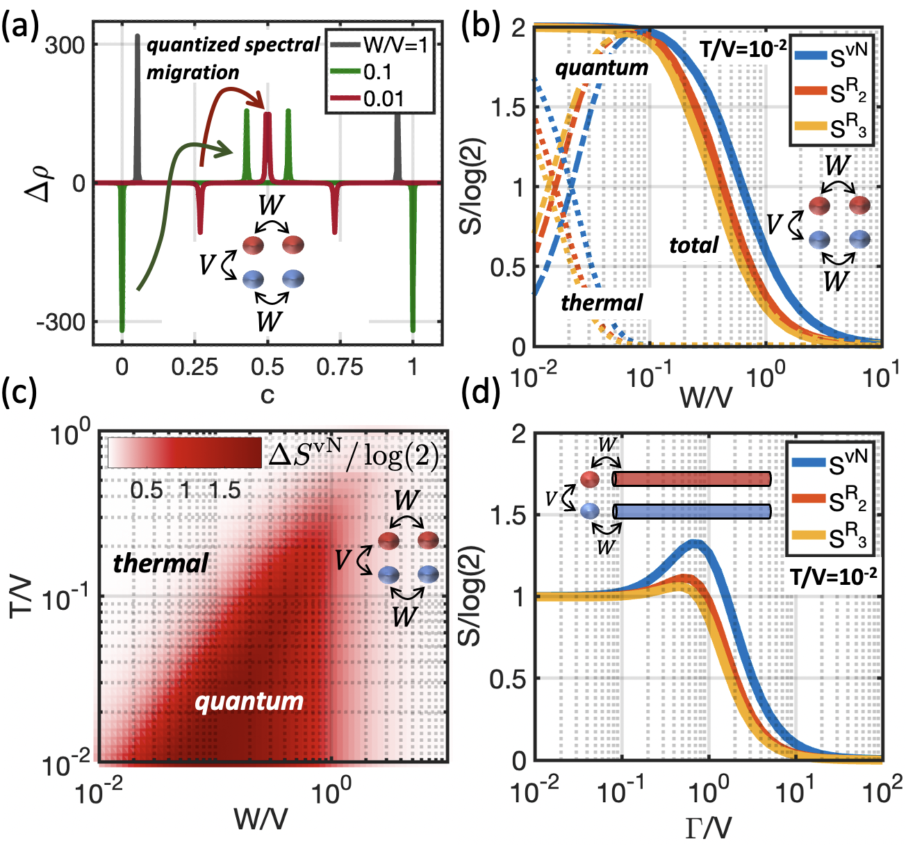
Figure 2: Free fermions coupled to (a-c) single-site and (d) wide-band bath geometries indicated in the insets. (a) Entanglement DoS $\Delta\rho(c)$ at $T/V=10^{-2}$ for various $W/V$ ratios, show a quantized migration of positive spectrum toward $c\to 1/2$ for $T<W$, followed by a negative spectrum migration at $W<T$. Each peak has a unit area. (b) von Neumann and Rényi EE as function of $W$ resolved into thermal part and quantum correction. (c) The quantum part of $S^{\rm vN}$ show its $W/T$ scaling. (d) von Neumann and Rényi EE as a function of $\Gamma/V$ for $\Gamma=\pi W^{2}/\Lambda$ in the large bandwidth $\Lambda$ limit.

The matrix $\mathbb{C}$ has to be discretized and diagonalized numerically. Assuming ${\cal N}$ frequency points, $\rho$ and $\rho_{0}$ are each ${\cal O}({\cal N})$, but $\Delta\rho$ is an ${\cal O}(1)$ zero-mean function, independent of frequency discretization [63]. The form of Eq. (15) is familiar from Luttinger’s theorem [64]. $\Delta\rho(c)$ consists of unit-area resonances located at $c$ values where the phase of determinant winds, corresponding to excess or deficit of an eigenvalue on top of a continuum.

Eqs. (14-15) indicate that the $\mathbb{C}$ part of the ES can be emulated by an infinite set of auxiliary particles $\tilde{\psi}_{a,\omega}$ in an extra dimension [57] in thermal equilibrium and occupations $\langle\tilde{\psi}^{\dagger}_{\omega}\tilde{\psi}^{\vphantom{\dagger}}_{\omega^{\prime}}\rangle=\mathbb{C}(\omega,\omega^{\prime})$ [65]. The relation $\mathbb{C}=(e^{\beta\tilde{\mathbb{H}}}-\tilde{\zeta})^{-1}$ defines entanglement Hamiltonian $\tilde{\mathbb{H}}$ [66].

In the non-interacting limit, the spectral function $\mathbb{A}^{a}(\omega)$ consists of a series of delta functions, which reduce the dimension of $\mathbb{C}$ to the number of modes. More importantly, $\Delta\rho<0$ contribution by $\mathbb{C}_{0}$ exactly cancels the thermal contribution to EE, $S_{a}$. In this limit $\tilde{\psi}_{a,\omega}\to\psi_{a}\delta(\omega)$, the matrix $\mathbb{C}$ represents occupation of real particles $\psi_{a}$, and our formalism reduces to known results [20]. See [60] for a detailed derivation.

Generally, when A-B coupling is weaker than temperature, Eq. (14) offers a perturbative expansion without the need to diagonalize $\mathbb{C}$ [60]. If the A-B coupling is irrelevant in a renormalization group sense, $\Sigma^{ab}\to 0$ and $\mathbb{J}_{A}\to 0$ and $\Delta S$ vanishes. On the other hand, if A-B coupling is relevant, for example in presence of edge modes in the energy spectrum of detached systems, $\Sigma^{ab}\to\infty$. In this case it is justified to flatten the spectrum [15] by neglecting the $k$-dependence of Green’s functions involved in computing $\mathbb{J}_{A}(\omega,\omega^{\prime})$. Writing $V^{2}=\Sigma^{ab}\Sigma^{ba}$, for each mode in A, $R^{aa^{\prime}}(z)\to\delta^{aa^{\prime}}V^{2}/(z-V^{2}/z)$ will have the same form as a two-site fermion problem with a coupling $V$. The latter has a zero mode in ES and an EE of $\log(2)$. The original model has a highly degenerate zero mode, whose degeneracy is lifted by $A^{a}(\omega)$, resulting in a gapless mode in ES, in apparent agreement with ETH [16].

At $T\to 0$ the negative part of $\Delta\rho$ can be ignored, and resonances can be represented by their entanglement ‘energies’ $\varepsilon=\log(1/c+\tilde{\zeta})$. An ES gap closing and re-opening with a zero mode then indicates a topological transition in the bulk and formation of edge states. Indeed the quantum EE $\Delta S/\log(2)=\rm{nullity}(\tilde{\mathbb{H}})$ is related to the number of zero modes of $\tilde{\mathbb{H}}$, a topological invariant.

In the rest of the paper we show that this formalism can be used to compute EE in large-N theories. For simplicity, we limit ourselves to two-site fermionic problems.

The simplest example is a system in which integrating out some internal degrees of freedom has led to a self-energy. Consider the four-site problem in a U geometry (inset of Fig. 2a) where A and B are coupled by $V$ but each are coupled by $W$ to a single-site bath, resulting in $\Sigma^{aa}(z)=\Sigma^{bb}(z)=W^{2}/z$. Fig. 2(b) shows EE in perfect agreement with exact diagonalization. At $W\to 0^{+}$, the bath sites are forced to be entangled, thus $S\to 2\log(2)$. Although the EE is constant for $W\ll V$, there is a crossover from quantum to thermal contributions as $W/T$ is varied [Fig. 2(c)]. Fig. 2(a) shows that at $W<V$ effectively two of the eigenvalues of $\mathbb{C}$ move to $c\to 1/2$, forming zero modes that increase EE to $2\log(2)$ but they are cancelled at $T<W$ by the spectral migration of $\mathbb{C}_{0}$ eigenvalues to zero. The EE decreases with increasing $W$, due to the entanglement monogamy.

Our technique readily generalizes to the case where A and B are decohered [67] by coupling to a fermionic bath [Fig. 2(d)], an example for which many other methods fail. In the wide-band limit the self-energy can be taken to be independent of frequency, i.e. $\Sigma(\omega+i\eta)=-i\Gamma$ for both sites. The resulting EE shows no inter-bath entanglement, but an overshoot at $\Gamma\sim V$ remains.

As an example of problems with self-consistency, we look at coupled-SYK models, defined as $H_{0}+H_{int}$ where

$$H_{0}=\frac{1}{4!}\sum_{\mu=A,B}\sum^{N_{\mu}}_{ijkl=1}J^{\mu}_{ijkl}\chi^{\mu}_{i}\chi^{\mu}_{j}\chi^{\mu}_{k}\chi^{\mu}_{l}.$$ (16)

$H_{0}$ describes two copies of SYK dots. Here, $\chi^{\mu}_{j}$ are Majorana fermions and $J^{\mu}_{ijkl}$ are random taken from a zero mean gaussian distribution (ZMGD) with the variance $J^{2}/N$. After disorder averaging and in the large-N_A,B limit this model reduces to a quadratic action with the two-point function that is determined self-consistently by the self-energy $\Sigma_{\mu}(\tau)=J^{2}G_{\mu}^{3}(\tau)$ and the Dyson equation $G_{\mu}^{-1}(z)=z-\Sigma_{\mu}(z)$. Readers are referred to [32, 68, 60] for important omitted aspects. Without coupling, $\Delta S_{A}=0$ and thus $S_{A}(T)=S^{\rm SYK}_{\rm th}(T)$, which at $T\to 0$ is given by the residual entropy of a single SYK.

One way of coupling the two dots is to consider the model $H=H_{0}+i\sum_{ij}V_{ij}\chi^{A}_{i}\chi^{B}_{j}$ [52, 53]. Assuming $N_{A}=N_{B}$, the simplest choice is then a constant $V_{ij}=V\delta_{ij}$. Considering that $\dim[\chi]=1/4$ for the SYK₄, this is a relevant coupling. The self-energy is given by

$$\Sigma_{\mu\nu}(\tau,\tau^{\prime})=J^{2}G_{\mu\nu}^{3}(\tau,\tau^{\prime})-V\tau_{\mu\nu}^{y}\delta(\tau,\tau^{\prime})$$ (17)

where indices $\mu$, $\nu$ are $a$ or $b$ for self-energy $\Sigma_{\mu\nu}$ and $A$ or $B$ for Green’s function $G_{\mu\nu}$ and $\tau^{y}$ is a Pauli matrix in A,B sectors. The model is known [52] to exhibit a first order transition which is holographically dual to the so-called Hawking-Page transition [69], describing instability of blackholes toward formation of a wormhole. We have solved this problem in real frequency [Fig. 3(b)] and found residual thermodynamical entropy. Surprisingly, we find $S^{\rm vN}_{A}=\frac{1}{2}\log 2$ mostly contributed by the thermal part. The $\Delta S_{A}^{\rm vN}$ is about half of the residual entropy.

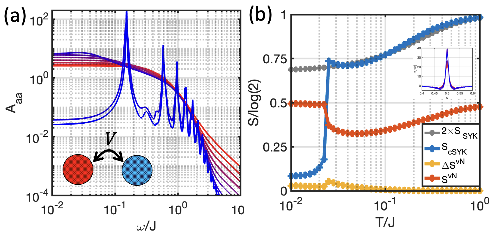
Figure 3: Coupled-SYK model with $V/J=0.075$. (a) Spectral function $A_{aa}$ for various temperatures, (b) Thermodynamic entropy $S_{\rm cSYK}$ and $S_{\rm SYK}$ of coupled- and single-SYK dots, as well as von Neumann EE $S^{\rm vN}_{A}$. Inset: EE DoS $\Delta\rho(c)$.

Alternatively, we may assume that $V_{ij}$ are random ZMGD [70, 71], or the two SYK dots are connected by four-fermion couplings $H=H_{0}+\sum_{ijkl}V_{ijkl}\chi_{i}^{A}\chi_{j}^{A}\chi_{k}^{B}\chi_{l}^{B}$, where $V_{ijkl}$ are again ZMGD with variance $V^{2}/N$. In this latter case, the self-consistency equations in the large-N limit becomes $(p=N_{A}/N_{B})$

$$\Sigma_{aa}(\tau)=J^{2}G_{AA}^{3}(\tau)+2V^{2}\sqrt{p}G^{2}_{BB}(\tau)G_{AA}(\tau)$$ (18)

and a similar equation for $\Sigma_{bb}$ with $A\leftrightarrow B$ and $p\to 1/p$. For $V=J$, this is a single SYK dot with $N=N_{A}+N_{B}$.

A common feature of all these four-fermion (as well as random two-fermion) coupling models is that the coupling is either marginal or irrelevant. Furthermore, $\Sigma^{ab}=\Sigma^{ba}=0$, and thus there are no quantum corrections $\Delta S_{A}=0$. The EE is given entirely by the thermal part $S^{vN}_{A}=S_{a}$, which is equal to the residual entropy of the SYK model $S_{0}(T_{\rm eff}/\tilde{J})$. Therefore, assuming equilibration, the thermalization is guaranteed.

In summary, we have provided a Green’s function formalism to compute ES of theories with a quadratic action through diagonalization of a single matrix built out of equilibrium functions. Interactions can be treated perturbatively within this formalism. However, we argued that this formalism provides access to the von Neumann EE of large-N theories. We applied our method to a non-interacting problem with self-energy as well as different forms of coupled SYK model. The method can be readily applied to Kondo lattices [30, 34, 35, 41] where changes in the pattern of entanglement are shown to be playing major role in Kondo breakdown transition [72, 73, 36]. Extension to non-equllibirium steady-state as well as quench dynamics is an interesting future direction.

Fruitful discussions with Y. Ge and R. Wijewardhana are appreciated.

Appendix

This appendix contains further details and extended proof of various statements in the paper.

.1 Non-interacting case

For the sake of completeness, we remind ourselves of the known non-interacting results [21, 20].

Bosons - The reduced density matrix is

$$\rho_{A}=\frac{e^{-H_{A}}}{Z_{A}}$$ (19)

where $H_{A}=\sum_{mn}\epsilon_{mn}a_{m}^{\dagger}a_{n}$ is the entanglement Hamiltonian and $Z_{A}=\prod_{k}({1-e^{\epsilon_{k}}})^{-1}$. We define the correlators

$$C_{mn}\equiv\langle a_{m}^{\dagger}a_{n}\rangle$$ (20)

The spectrum of $\mathbb{C}$ and $H_{A}$ have the following relation

$$\nu_{k}=\frac{1}{e^{\epsilon_{k}}-1}$$ (21)

where $\{\nu_{k}\}$ is the spectrum of $\mathbb{C}$ and $\{\epsilon_{k}\}$ is spectrum of $H_{A}$. The von Neumann entropy and Rényi entropy are

$$S^{\rm vN}_{A} = -{\rm Tr}\left[\rho_{A}\ln{\rho_{A}}\right]$$

$$= \sum_{k}\Big{[}\frac{\epsilon_{k}e^{-\epsilon_{k}}}{1-e^{-\epsilon_{k}}}-\ln(1-e^{-\epsilon_{k}})\Big{]},$$

and

$$S^{{\rm R}_{M}}_{A}=\frac{{\rm Tr}\left[\ln\rho_{A}^{M}\right]}{1-M}$$ (23)

Instead of using the spectrum $\{\epsilon\}$, one can use the spectrum $\{\nu_{k}\}$ to calculate von Neumann entropy and Rényi entropy as

$$S^{\rm vN}_{A}=\sum_{k}(1+\nu_{k})\ln(1+\nu_{k})-\nu_{k}\ln\nu_{k}$$ (24)

and

$$S^{{\rm R}_{M}}_{A}={\rm Tr}\ln\Big{[}(1+\nu_{k})^{M}-\nu_{k}^{M}\Big{]}.$$ (25)

or equivalently in terms of the C matrix as

$$S^{\rm vN}_{A}=-{\rm Tr}\left[(\mathbb{1}+\mathbb{C})\ln(\mathbb{1}+\mathbb{C})-\mathbb{C}\ln\mathbb{C}\right]$$ (26)

and

$$S^{{\rm R}_{M}}_{A}=-\frac{1}{1-M}\ln\det\Big{[}(\mathbb{1}+\mathbb{C})^{M}-\mathbb{C}^{M}\Big{]}.$$ (27)

Fermions - The entanglement Hamiltonian is

$$\rho_{A}=\frac{e^{-H_{A}}}{Z_{A}}$$ (28)

where $H_{A}=\sum_{mn}\epsilon_{mn}a_{m}^{\dagger}a_{n}$ and $Z_{A}=\prod_{k}(1+e^{-\epsilon_{k}})$. Again, we define the correlator

$$C_{mn}\equiv\langle a_{m}^{\dagger}a_{n}\rangle$$ (29)

The spectrum of $\mathbb{C}$ and $H_{A}$ are related according to

$$\nu_{k}=\frac{1}{e^{\epsilon_{k}}+1}$$ (30)

where $\{\nu_{k}\}$ is the spectrum of $\mathbb{C}$ and $\{\epsilon_{k}\}$ is spectrum of $H_{A}$. Therefore, von Neumann entropy and Rényi entropy are

$$S^{\rm vN}_{A}=-{\rm Tr}\left[\rho_{A}\ln{\rho_{A}}\right]=\sum_{k}\Big{(}\frac{\epsilon_{k}e^{-\epsilon_{k}}}{1+e^{-\epsilon_{k}}}+\ln(1+e^{-\epsilon_{k}})\Big{)},$$ (31)

and

$$S^{{\rm R}_{M}}_{A}=\frac{1}{1-M}\ln{\rm Tr}\left[\rho_{A}^{M}\right].$$ (32)

Instead of using the spectrum $\{\epsilon\}$, one can use the spectrum $\{\nu_{k}\}$ to calculate von Neumann entropy and Rényi entropy as

$$S^{\rm vN}_{A}=-\sum_{k}(1-\nu_{k})\ln(1-\nu_{k})+\nu_{k}\ln\nu_{k}$$ (33)

and

$$S^{{\rm R}_{M}}_{A}=tr\ln\Big{[}(1+\nu_{k})^{M}-\nu_{k}^{M}\Big{]}$$ (34)

which in terms of the $C$-matrix are given by or

$$S^{\rm vN}_{A}=-{\rm Tr}\left[(1-\mathbb{C})\ln(1-\mathbb{C})+\mathbb{C}\ln\mathbb{C}\right]$$ (35)

and

$$S^{{\rm R}_{M}}_{A}=\frac{1}{1-M}\ln\det\Big{[}(\mathbb{1}-\mathbb{C})^{M}+\mathbb{C}^{M}\Big{]}.$$ (36)

We can unify the entropies of Bosons and Fermions into the following

$$S^{\rm vN}_{A}=\zeta{\rm Tr}\left[(\mathbb{1}+\tilde{\zeta}\mathbb{C})\ln(\mathbb{1}+\tilde{\zeta}\mathbb{C})-\tilde{\zeta}\mathbb{C}\ln\mathbb{C}\right]$$ (37)

and

$$S^{{\rm R}_{M}}_{A}=\frac{-\zeta}{1-M}\ln\det\Big{[}(\mathbb{1}+\tilde{\zeta}\mathbb{C})^{M}-\tilde{\zeta}\mathbb{C}^{M}\Big{]}.$$ (38)

.2 Replica symmetry and self-energy

In order to compute the Rényi entropy, one need to solve the large-N path-integral problem on an extended manifold shown in Fig. 1(c). The Rényi entropy is given by

$${\rm Tr}\left[\rho_{A}^{M}\right]=\frac{1}{Z^{M}}\int{D[G,\Sigma]D\chi}e^{-N{\cal S}[\chi,G,\Sigma]}$$ (39)

here, $\chi$ represents the fermions and $G-\Sigma$ are used to decouple the interaction. Here, we show how this problem reduces to the action (4) and (6) of the paper. In order to be concrete and without loss of generality, we consider the coupled SYK model [52]. This equilibrium path integral description of this model is reviewed in section .8.1 of the present supplementary materials. The replica action is

$${\cal S}=\sum_{\mu,\nu=A,B}\sum_{r}\int d\tau\Bigg{\{}\frac{1}{2N}\sum_{i=1}^{N}\chi^{(r)}_{i,\mu}(\tau)[\partial_{\tau}\delta_{\mu\nu}+V\tau^{y}_{\mu\nu}]\chi^{(r)}_{i,\nu}(\tau^{\prime})+\delta_{\mu\nu}\frac{J^{\mu}_{i,j,k,l}}{4!}\sum_{i,j,k,l=1}^{N}\chi^{(r)}_{i,\mu}\chi^{(r)}_{j,\mu}\chi^{(r)}_{k,\mu}\chi^{(r)}_{l,\mu}\Bigg{\}}\\$$ (40)

which is diagonal in replica and needs to be supplemented with the boundary condition (2). $\tau^{y}$ is a Pauli matrix and the random variables $J^{\mu}_{ijkl}$ have zero mean and the variance

$$J^{\mu}_{ijkl}J^{\nu}_{i^{\prime}j^{\prime}k^{\prime}l^{\prime}}=\delta^{\mu\nu}\delta_{ii^{\prime}}\delta_{jj^{\prime}}\delta_{kk^{\prime}}\delta_{ll^{\prime}}\frac{J^{2}}{4N^{3}}$$ (41)

After disorder averaging, the action develops off-diagonal-in-replica contributions and after $G-\Sigma$ decoupling becomes

$${\cal S} = \sum_{r,r^{\prime}}\sum_{\mu\nu=A,B}\int d\tau d\tau^{\prime}\Bigg{\{}\frac{1}{2N}\sum_{i}\chi^{(r)}_{i,\mu}(\tau)[\partial_{\tau}\delta(\tau,\tau^{\prime})\delta_{\mu\nu}\delta^{rr^{\prime}}+\Sigma^{(rr^{\prime})}_{\mu\nu}(\tau,\tau^{\prime})]\chi^{(r^{\prime})}_{i,\nu}(\tau^{\prime})$$

$$\hskip 56.9055pt-\frac{1}{2}\Big{[}\Big{(}\Sigma^{(rr^{\prime})}_{\mu\nu}(\tau,\tau^{\prime})-V\tau^{y}_{\mu\nu}\delta(\tau,\tau^{\prime})\delta^{rr^{\prime}}\Big{)}G^{(r^{\prime}r)}_{\nu\mu}(\tau^{\prime},\tau)+\frac{J^{2}}{4}[G^{(rr^{\prime})}_{\mu\nu}(\tau,\tau^{\prime})]^{4}\Big{]}\Bigg{\}}$$

where $\mu$ and $\nu$ are $a$ or $b$ for self-energy $\Sigma_{\mu\nu}$ and $A$ or $B$ for Green’s function $G_{\mu\nu}$. Note that the interacting part of the action contains inter-replica interaction and such four-fermion terms are decoupled by the $G^{(rr^{\prime})}$ Green’s function, leading to off-diagonal replica self-energy $\Sigma^{(rr^{\prime})}$. Transforming from the replica sector $n$, to replica momentum space $p$, we find

$${\cal S} = \sum_{p,p^{\prime}}\sum_{\mu\nu=A,B}\int d\tau d\tau^{\prime}\Big{\{}\frac{1}{2N}\sum_{i}\bar{\chi}^{(p)}_{i,\mu}(\tau)\left(\partial_{\tau}\delta(\tau,\tau^{\prime})\delta_{\mu\nu}\delta^{pp^{\prime}}+\Sigma^{(pp^{\prime})}_{\mu\nu}(\tau,\tau^{\prime})\right)\chi^{(p^{\prime})}_{i,\nu}(\tau^{\prime})$$

$$-\frac{1}{2}\sum_{\mu\nu}\Big{[}\Big{(}\Sigma^{(pp^{\prime})}_{\mu\nu}(\tau^{\prime},\tau)-V\tau^{y}_{\mu\nu}\delta^{pp^{\prime}}\delta(\tau,\tau^{\prime})\Big{)}G^{(pp^{\prime})}_{\nu\mu}(\tau,\tau^{\prime})$$

$$+\frac{J^{2}}{4M^{2}}\sum_{p_{1},p_{2},p_{3},p_{1}^{\prime},p_{2}^{\prime},p_{3}^{\prime}}G^{(p_{1}p_{1}^{\prime})}_{\mu\nu}(\tau,\tau^{\prime})G^{(p_{2}p_{2}^{\prime})}_{\mu\nu}(\tau,\tau^{\prime})G^{(p_{3}p_{3}^{\prime})}_{\mu\nu}(\tau,\tau^{\prime})G^{(-p_{1}-p_{2}-p_{3},-p_{1}^{\prime}-p_{2}^{\prime}-p_{3}^{\prime})}_{\mu\nu}(\tau,\tau^{\prime})\Big{]}\Big{\}}$$

where we have used

$$\chi^{(r)}(\tau)=\frac{1}{\sqrt{M}}\sum_{p}\Omega^{pr}\chi^{(p)}(\tau),\quad G^{(rr^{\prime})}(\tau,\tau^{\prime})=\frac{1}{M}\sum_{pp^{\prime}}\Omega^{pr-p^{\prime}r^{\prime}}G^{(pp^{\prime})}(\tau,\tau^{\prime}),\quad\Sigma^{(r)}(\tau,\tau^{\prime})=\frac{1}{M}\sum_{pp^{\prime}}\Omega^{-(pr-p^{\prime}r^{\prime})}\Sigma^{(pp^{\prime})}(\tau,\tau^{\prime}),$$ (43)

with inverse relations

$$\chi^{(p)}(\tau)=\frac{1}{\sqrt{M}}\sum_{r}\Omega^{-pr}\chi^{(r)}(\tau),\quad G^{(pp^{\prime})}(\tau,\tau^{\prime})=\frac{1}{M}\sum_{rr^{\prime}}\Omega^{-(pr-p^{\prime}r^{\prime})}G^{(r)}(\tau,\tau^{\prime}),\quad\Sigma^{(p)}(\tau,\tau^{\prime})=\frac{1}{M}\sum_{rr^{\prime}}\Omega^{(pr-p^{\prime}r^{\prime})}\Sigma^{(r)}(\tau,\tau^{\prime}).$$ (44)

Now in the $p$ space, one set of saddle point solutions are found by varying the Green’s function $G^{(pp^{\prime})}_{\mu\nu}$

$$\Sigma^{(pp^{\prime})}_{\mu\nu}(\tau^{\prime},\tau)=-\frac{J^{2}}{M^{2}}\sum_{p_{1},p_{2},p_{1}^{\prime},p_{2}^{\prime}}G^{(p_{1}p_{1}^{\prime})}_{\mu\nu}(\tau,\tau^{\prime})G^{(p_{2}p_{2}^{\prime})}_{\mu\nu}(\tau,\tau^{\prime})G^{(-p_{1}-p_{2}-p,-p_{1}^{\prime}-p_{2}^{\prime}-p^{\prime})}_{\mu\nu}(\tau,\tau^{\prime})-V\tau^{y}_{\mu\nu}\delta^{pp^{\prime}}\delta(\tau,\tau^{\prime})$$ (45)

The variations w.r.t $\Sigma^{(pp^{\prime})}_{\mu\nu}$ gives the the Dyson equation

$$G^{(p^{\prime}p)}(\tau,\tau^{\prime})=\frac{1}{N}\sum_{i}\left\langle\chi_{i}^{(p)}(\tau^{\prime})\chi^{(p^{\prime})}_{i}(\tau)\right\rangle={\cal G}_{p,p^{\prime}}(\tau,\tau^{\prime}).$$ (46)

We note that while these equations do generally support replica off-diagonal solutions $G^{(pp^{\prime})}$ and $\Sigma^{(pp^{\prime})}$, However, replica symmetry is also preserved by these equations. This means if we assume $G^{(pp^{\prime})}\propto\delta^{pp^{\prime}}$ we find $\Sigma^{(pp^{\prime})}\propto\delta^{pp^{\prime}}$ which means the action decouples into different $p$ sectors, leading to $G^{(pp^{\prime})}\propto\delta^{pp^{\prime}}$. Considering that the at UV, $G\sim J\delta^{pp^{\prime}}$ is replica symmetric, we conclude that the replica symmetry is preserved. Therefore, the Green’s functions and self-energies can be represented by online diagonal $p$ indices, $G^{(p)}(\tau,\tau^{\prime})={\cal G}_{p}(\tau,\tau^{\prime})$. Likewise, the self consistency equations become the same for different $p$ sectors:

$$\Sigma^{(p)}_{\mu\mu}(\tau^{\prime},\tau)=-\frac{J^{2}}{M^{2}}\sum_{p_{1}p_{2}}G^{(p_{1})}_{\mu\mu}(\tau,\tau^{\prime})G^{(p_{2})}_{\mu\mu}(\tau,\tau^{\prime})G^{(-p-p_{1}-p_{2})}_{\mu\mu}(\tau,\tau^{\prime})-V\tau^{y}_{\mu\nu}\delta(\tau,\tau^{\prime})$$ (47)

The only thing different between various sectors is the boundary condition in imaginary-time direction. So, a full solution to the problem requires simultaneous solution to all $p$ sectors. Eventually, the ${\rm Tr}\left[\rho^{M}_{A}\right]$ can be written as

$${\rm Tr}\left[\rho^{M}_{A}\right]=\frac{1}{Z_{0}^{M}}\int{D\chi}e^{-N{\cal S}},\qquad{\cal S}={\cal S}_{Q}+{\cal S}_{C}$$ (48)

where using the saddle-point equations, the classical part is

$${\cal S}_{C}=-\sum_{p}\int d\tau d\tau^{\prime}\frac{1}{2}\sum_{\mu\nu}\Big{[}\frac{3}{4}\Big{(}\Sigma^{(p)}_{\mu\nu}(\tau,\tau^{\prime})-V\tau^{y}_{\mu\nu}\delta(\tau,\tau^{\prime})\Big{)}G^{(p)}_{\nu\mu}(\tau^{\prime},\tau)\Big{]}.$$ (49)

and the quantum part of the action is

$${\cal S}_{Q}=\sum_{p}\sum_{\mu\nu=A,B}\int d\tau d\tau^{\prime}\Big{\{}\frac{1}{2N}\sum_{i}\bar{\chi}^{(p)}_{i,\mu}(\tau)\left(\partial_{\tau}\delta(\tau,\tau^{\prime})\delta_{\mu\nu}+\Sigma^{(p)}_{\mu\nu}(\tau,\tau^{\prime})\right)\chi^{(p)}_{i,\nu}(\tau^{\prime}).$$ (50)

As we have argued in the paper, however, a full self-consistent solution to all $p$-sectors is not needed if we are only interested in the von Neumann entanglement entropy. In this case, we could assume that the self-energy $\Sigma^{(p)}(\tau,\tau^{\prime})=\Sigma(\tau_{1}-\tau_{2})$ has the same expression as the time-translational invariant $p=0$ sector. Going to frequency space, the quantum action becomes

$${\cal S}_{Q} = \frac{1}{2N}\sum_{p}\sum_{i}\sum_{n,m,n^{\prime},m^{\prime}}\left[\begin{array}[]{cc}\bar{\chi}^{(p)}_{A,i}(i\bar{\omega}_{n})&\bar{\chi}^{(p)}_{B,i}(i\omega_{m})\end{array}\right]\left(\begin{array}[]{cc}-i\bar{\omega}_{n}+\Sigma_{nn^{\prime}}^{aa}&\Sigma_{nm^{\prime}}^{ab}\\ \Sigma_{mn^{\prime}}^{ba}&-i\omega_{m}+\Sigma_{mm^{\prime}}^{bb}\end{array}\right)\left[\begin{array}[]{c}\chi^{(p)}_{A,i}(i\bar{\omega}_{n^{\prime}})\\ \chi^{(p)}_{B,i}(i\omega_{m^{\prime}})\end{array}\right]$$ (56)

where $n,n^{\prime}$ and indices for shifted Matsubara frequencies, different in each $p$ sector and $m,m^{\prime}$ are indices for normal Matsubara frequencies. The elements of self-energies are worked out in section .3.

Then $G$ and $\Sigma$ will be just the equilibrium Green’s functions and self-energies with $p=0$.

.3 Construction of the action in the replica-momentum space

In this section, we construct the elements of the matrix ${\cal G}_{u}^{-1}$ appearing in action (4) of the paper. The diagonal elements are quite straight forward, so we focus on off-diagonal elements for both bosons and fermions. We use the following identities

$$\Sigma(\tau)=\frac{1}{\beta}\sum_{n}\Sigma(i\omega_{n})e^{-i\omega_{n}\tau},\quad\Sigma(z)=\int{\frac{dx}{\pi}}\frac{\Sigma^{\prime\prime}(x)}{x-z}.$$

Fermions - For the case of fermions we can write

$$\Sigma(\tau) = -\oint{\frac{dz}{2\pi i}}[f(z)-\theta_{\tau>0}]e^{-z\tau}\int{\frac{dx}{\pi}}\frac{\Sigma^{\prime\prime}(x)}{x-z}$$ (57)

$$= \int{\frac{dx}{\pi}}[f(x)-\theta_{\tau>0}]\Sigma^{\prime\prime}(x)e^{-x\tau}$$

Note that $\theta_{\tau>0}$ is important for convergence, but also necessary to make sure that the Green’s function is $\beta$ anti-periodic. The two-point version is simple but note that $\Sigma(\tau_{1},\tau)=T\Sigma(\tau_{1}-\tau_{2})$. Then,

$$\Sigma_{nm^{\prime}} = T\int_{0}^{\beta}{d\tau_{1}d\tau_{2}}e^{i(\bar{\omega}_{n}\tau_{1}-\omega_{m^{\prime}}\tau_{2})}\Sigma(\tau_{1}-\tau_{2})$$ (58)

The result is

$$\Sigma_{nm^{\prime}} = T\frac{1+u}{i\bar{\omega}_{n}-i\omega_{m^{\prime}}}\int{\frac{dx}{\pi}}\frac{\Sigma^{\prime\prime}(x)}{i\omega_{m^{\prime}}-x}$$ (59)

$$= -T\frac{1+u}{i\bar{\omega}_{n}-i\omega_{m^{\prime}}}\Sigma(i\omega_{m^{\prime}}),$$

where $u=e^{i\bar{\omega}_{n}\beta}$. Note that choosing $\Sigma(\tau_{1},\tau_{2})=V\delta(\tau_{1},\tau_{2})$ or $\Sigma(i\omega_{m^{\prime}})=V$ reproduces the known result:

$$V\int_{0}^{\beta}{d\tau e^{i(\bar{\omega}_{n}-\omega_{m^{\prime}})\tau}}=-\frac{1}{\beta}V\frac{u+1}{i\bar{\omega}_{n}-i\omega_{m^{\prime}}}.$$ (60)

Similarly, we can show that

$$\Sigma_{mn^{\prime}}=-T\frac{1+u^{-1}}{i\omega_{m}-i\bar{\omega}_{n^{\prime}}}\Sigma(i\omega_{m}).$$ (61)

This is correct, because using $\bar{\omega}_{n}=\nu_{n}-iT\log u$ we find

$$\lim_{u\to-1}\Sigma_{nm^{\prime}} = \lim_{\epsilon\to 0}\frac{-T\epsilon\delta_{nm^{\prime}}\Sigma(i\omega_{m^{\prime}})}{T\log(-1+\epsilon)-i\pi T}=\delta_{nm^{\prime}}\Sigma(i\omega_{m^{\prime}}),$$

$$\lim_{u\to-1}\Sigma_{mn^{\prime}} = \lim_{\epsilon\to 0}\frac{-T[(-1+\epsilon)^{-1}+1]\delta_{mn^{\prime}}\Sigma(i\omega_{m})}{i\pi T-T\log(-1+\epsilon)},$$

$$=\delta_{mn^{\prime}}\Sigma(i\omega_{m}).$$

Bosons - In this case we have

$$\Sigma(\tau) = \frac{1}{\beta}\sum_{n}e^{-i\nu_{n}\tau}\Sigma(i\nu_{n})$$ (62)

$$= \oint{\frac{dz}{2\pi i}}[n(z)+\theta_{\tau}]e^{-z\tau}\Sigma(z)$$

$$= \int{\frac{dx}{\pi}}\Sigma^{\prime\prime}(x)[n(x)+\theta_{\tau}]e^{-x\tau}$$

This has the correct half-periodicity, as seen in

$$\Sigma(\beta-\left|\tau\right|) = \int{\frac{dx}{\pi}}\Sigma^{\prime\prime}(x)[n(x)+1]e^{-\beta x}e^{+x\left|\tau\right|}$$

$$= \int{\frac{dx}{\pi}}\Sigma^{\prime\prime}(x)n(x)e^{+x\left|\tau\right|}=\Sigma(-\left|\tau\right|)$$

Fourier transform is

$$\Sigma_{nm^{\prime}} = T\int{\frac{dx}{\pi}\Sigma^{\prime\prime}(x)}\int_{0}^{\beta}{d\tau_{1}d\tau_{2}}[n(x)+\theta_{\tau_{1}>\tau_{2}}]$$

$$\hskip 128.0374pte^{i(\bar{\omega}_{n}-x)\tau_{1}}e^{-(i\nu_{m^{\prime}}-x)\tau_{2}}$$

$$= T\frac{u-1}{i\bar{\omega}_{n}-i\nu_{m^{\prime}}}\int{\frac{dx}{\pi}\frac{\Sigma^{\prime\prime}(x)}{x-i\nu_{m^{\prime}}}}=T\frac{u-1}{i\bar{\omega}_{n}-i\nu_{m^{\prime}}}\Sigma(i\nu_{m^{\prime}})$$

and

$$\Sigma_{mn^{\prime}} = T\int{\frac{dx}{\pi}\Sigma^{\prime\prime}(x)}\int_{0}^{\beta}{d\tau_{1}d\tau_{2}}[n(x)+\theta_{\tau_{1}>\tau_{2}}]$$

$$\hskip 128.0374pte^{-i(\bar{\omega}_{n^{\prime}}-x)\tau_{2}}e^{(i\nu_{m}-x)\tau_{1}}$$

$$= T\frac{u^{-1}-1}{i\nu_{m}-i\bar{\omega}_{n^{\prime}}}\int{\frac{dx}{\pi}\frac{\Sigma^{\prime\prime}(x)}{x-i\nu_{m}}}=T\frac{u^{-1}-1}{i\nu_{m}-i\bar{\omega}_{n^{\prime}}}\Sigma(i\nu_{m}).$$

As a check, using $e^{i\beta\bar{\omega}_{n}}=u$ and $\bar{\omega}_{n}=\nu_{n}-iT\log u$ we find

$$\lim_{u\to 1}\Sigma_{mn^{\prime}}=\delta_{mn^{\prime}}\Sigma(i\nu_{m}),\qquad\lim_{u\to 1}\Sigma_{nm^{\prime}}=\delta_{nm^{\prime}}\Sigma(i\nu_{m^{\prime}})$$

So, in summary

$$\Sigma_{nm^{\prime}}=-\frac{1}{\beta}\frac{\tilde{\zeta}u+1}{i\bar{\omega}_{n}-i\omega_{m^{\prime}}},\qquad\Sigma_{mn^{\prime}}=-\frac{1}{\beta}\frac{\tilde{\zeta}u^{-1}+1}{i\omega_{m}-i\bar{\omega}_{n^{\prime}}}.$$ (63)

.4 Useful matrix identities

In this section, we provide some useful matrix identities that are used in the paper. The first is the famous determinant identity

$$\det\left[\begin{array}[]{c|c}A&B\\ \hline\cr C&D\end{array}\right] = \det(A)\det(D-BA^{-1}C)$$

$$= \det(D)\det(A-CD^{-1}B)$$

which leads to the equation employed in the paper:

$$\det\left[\begin{array}[]{c|c}I_{mm}&V_{mn}\\ \hline\cr V_{nm}&I_{nn}\end{array}\right] = \det(I_{mm}-V_{mn}V_{nm})$$

$$= \det(I_{nn}-V_{nm}V_{mn}).$$

We also use some matrix inversion identities. If $(A-BD^{-1}C)$ is invertible

$$\left[\begin{array}[]{cc}A&B\\ C&D\end{array}\right]^{-1}=\left[\begin{array}[]{cc}(A-BD^{-1}C)^{-1}&-(A-BD^{-1}C)^{-1}BD^{-1}\\ -D^{-1}C(A-BD^{-1}C)^{-1}&D^{-1}+D^{-1}C(A-BD^{-1}C)^{-1}BD^{-1}\end{array}\right]$$ (70)

If $(D-CA^{-1}B)$ is invertible

$$\left[\begin{array}[]{cc}A&B\\ C&D\end{array}\right]^{-1}=\left[\begin{array}[]{cc}A^{-1}+A^{-1}B(D-CA^{-1}B)^{-1}CA^{-1}&-A^{-1}B(D-CA^{-1}B)^{-1}\\ -(D-CA^{-1}B)^{-1}CA^{-1}&(D-CA^{-1}B)^{-1}\end{array}\right]$$ (71)

A consequence of these identities is that

$$V_{qk}G^{B}_{kk^{\prime}}V_{k^{\prime}q} = V_{qk}(G_{b}^{-1}-V_{kq}G_{a}V_{qk})^{-1}V_{kq}=\left(\begin{array}[]{cc}V_{qk}&0\end{array}\right)\left(\begin{array}[]{cc}G_{b}^{-1}&V_{kq}\\ V_{qk}&G_{a}^{-1}\end{array}\right)\left(\begin{array}[]{cc}V_{kq}\\ 0\end{array}\right)$$

$$= V_{qk}[G_{b}+G_{b}V_{qk}(g_{A}^{-1}-V_{qk}G_{b}V_{kq})^{-1}V_{qk}G_{b}]V_{kq}$$

$$= \Sigma_{a}+\Sigma_{a}G_{A}\Sigma_{a}=G_{a}^{-1}G_{A}G_{a}^{-1}-G_{a}^{-1}$$ (78)

.5 A more detailed proof of Eq. (9)

Here, we provide a more detailed proof of central equation of the paper, Eq. (9). We start from the action (4)

$${\cal S} = \frac{1}{\beta}\sum_{n}\Big{[}\bar{\psi}_{a}(i\bar{\omega}_{n})\Big{(}-i\bar{\omega}_{n}+\epsilon_{a}+\Sigma^{aa}(i\bar{\omega}_{n})\Big{)}\psi_{a}(i\bar{\omega}_{n})+\sum_{m}\bar{\psi}_{b}(i\omega_{m})\Big{(}-i\omega_{m}+\epsilon_{b}+\Sigma^{bb}(i\omega_{m})\Big{)}\psi_{b}(i\omega_{m})$$

$$\hskip 56.9055pt+\frac{1}{\beta^{2}}\sum_{n,m}\Big{\{}\Sigma^{ab}(i\omega_{m})\frac{e^{i\bar{\omega}_{n}\beta}-1}{i\bar{\omega}_{n}-i\omega_{m}}\bar{\psi}_{a}(i\bar{\omega}_{n})\psi_{b}(i\omega_{m})+\Sigma^{ba}(i\omega_{m})\frac{e^{-i\bar{\omega}_{n}\beta}-1}{i\omega_{m}-i\bar{\omega}_{n}}\bar{\psi}_{b}(i\omega_{m})\psi_{a}(i\bar{\omega}_{n})\Big{\}}\Big{]}$$

Shift $\psi_{a}(i\bar{\omega}_{n})\to\psi_{a}(i\bar{\omega}_{n})-\frac{1}{\beta}\sum_{m}\Sigma^{ba}(i\omega_{m})\frac{1}{i\bar{\omega}_{n}-\epsilon_{a}-\Sigma_{aa}(i\bar{\omega}_{n})}\frac{1-u^{-1}}{i\bar{\omega}_{n}-i\omega_{m}}\psi_{b}(i\omega_{m})$, the action becomes

$${\cal S} = {\cal S}_{A}+\frac{1}{\beta^{2}}\sum_{m,m^{\prime},n}\bar{\psi}_{b}(i\omega_{m})\Big{[}-[G^{-1}(i\omega_{m})]^{bb^{\prime}}\delta_{m,m^{\prime}}$$

$$\hskip 56.9055pt+\frac{1}{\beta}\Sigma^{ba}(i\omega_{m})\frac{1}{i\bar{\omega}_{n}-\epsilon_{a}-\Sigma^{aa^{\prime}}(i\bar{\omega}_{n})}\frac{(1-u)(1-u^{-1})}{(i\bar{\omega}_{n}-i\omega_{m})(i\bar{\omega}_{n}-i\omega_{m^{\prime}})}\Sigma^{a^{\prime}b^{\prime}}(i\omega_{m^{\prime}})\Big{]}\psi_{b}(i\omega_{m^{\prime}})$$

where $[G^{-1}(i\omega_{m})]^{bb^{\prime}}=-i\omega_{m}+\epsilon_{b}+\Sigma^{bb^{\prime}}(i\omega_{m})$. Using spectral representation

$${\cal S}={\cal S}_{A}+\frac{1}{\beta^{2}}\sum_{m,m^{\prime}}\bar{\psi}_{b}(i\omega_{m})\Big{[}-[G^{-1}(i\omega_{m})]^{bb^{\prime}}\delta_{m,m^{\prime}}+\frac{1}{\beta}\sum_{n}\Sigma^{ba}(i\omega_{m})\int\frac{dx}{2\pi}\frac{A^{aa^{\prime}}(x)}{i\bar{\omega}_{n}-x}\frac{(1-u)(1-u^{-1})}{(i\bar{\omega}_{n}-i\omega_{m})(i\bar{\omega}_{n}-i\omega_{m^{\prime}})}\Sigma^{a^{\prime}b^{\prime}}(i\omega_{m^{\prime}})\Big{]}\psi_{b}(i\omega_{m^{\prime}})\\$$ (79)

After integrating out the shifted Matsubara frequency, the action becomes

$${\cal S} = {\cal S}_{A}+\frac{1}{\beta^{2}}\sum_{m,m^{\prime}}\bar{\psi}_{b}(i\omega_{m})\Big{[}-[G^{-1}(i\omega_{m})]^{BB^{\prime}}\delta_{m,m^{\prime}}$$

$$+\int{\frac{dx}{2\pi}}\frac{K_{u}(x)\Sigma^{ba}(i\omega_{m})A^{aa^{\prime}}(x)\Sigma^{a^{\prime}b}(i\omega_{m^{\prime}})}{(i\omega_{m}-x)(i\omega_{m^{\prime}}-x)}\Big{]}\psi_{b}(i\omega_{m^{\prime}})$$

where $-[G^{-1}(i\omega_{m})]^{BB^{\prime}}$ is

$$-[G^{-1}(i\omega_{m})]^{bb^{\prime}}+\int\frac{dx}{2\pi}\frac{\Sigma^{ba}(i\omega_{m})A^{aa^{\prime}}(x)\Sigma^{a^{\prime}b^{\prime}}(i\omega_{m})}{i\omega_{n}-x}$$ (81)

Then the whole second part in action $S$ gives $({\cal G}_{u}^{BB^{\prime}})^{-1}$ which is

$$[G^{-1}_{m}]^{BB^{\prime}}\delta_{mm^{\prime}}-\int{\frac{dx}{2\pi}}\frac{K_{u}(x)\Sigma^{ba}_{m}A^{aa^{\prime}}(x)\Sigma^{a^{\prime}b^{\prime}}_{m^{\prime}}}{\beta(i\omega_{m}-x)(i\omega_{m^{\prime}}-x)}$$ (82)

The determinant $\det{}^{-\zeta}[(-{\cal G}_{u}^{BB^{\prime}})^{-1}]$ now is

$$\det{}^{-\zeta}\Big{[}[G^{-1}_{m}]^{BB^{\prime}}\delta_{mm^{\prime}}-\int{\frac{dx}{2\pi}}\frac{K_{u}(x)\Sigma^{ba}_{m}A^{aa^{\prime}}(x)\Sigma^{a^{\prime}b^{\prime}}_{m^{\prime}}}{\beta(i\omega_{m}-x)(i\omega_{m^{\prime}}-x)}\Big{]}$$ (83)

Now we are facing a determinant

$$\det{}^{-\zeta}\Big{[}D_{mm^{\prime}}\delta_{mm^{\prime}}+\sum_{x}w_{m}(x)v^{T}_{m^{\prime}}(x)\Big{]}$$ (84)

This is nothing but

where $N_{x}$, $N_{a}$ and $N_{m}$ refer to the number of real frequencies, number of A modes and number of Matsubara frequencies, respectively. Then the determinant is

$$\det{}^{-\zeta}\Big{[}\delta(x,y)\delta_{aa^{\prime}}+\sum_{m}v^{T}_{m}(x,a)D_{mm}w_{m}(y,a^{\prime})\Big{]}$$ (85)

Using Eq. (.4), and after the shuffling the determinant becomes

$$\det{}^{-\zeta}\Big{[}\delta(x,y)$$

$$\hskip 28.45274pt-\frac{1}{\beta}\sum_{m}K_{u}(x)A^{a}(x)\frac{\Delta x}{2\pi}\frac{\Sigma_{m}^{ab}G_{m}^{BB^{\prime}}\Sigma_{m}^{ba}}{(i\omega_{m}-x)(i\omega_{m}-y)}\Big{]}$$

This motivates defining [$z$ is the complex frequency]

$$\mathbb{R}(z)\equiv\Sigma^{ab}(z)G^{BB^{\prime}}(z)\Sigma^{ba}(z)$$ (86)

in terms of which

$$\mathbb{r}(x) \equiv \frac{1}{\beta}\sum_{n}\frac{\mathbb{R}(i\omega_{n})}{i\omega_{n}-x}$$ (87)

$$= \int\frac{d\omega}{2\pi}\mathbb{A}_{R}(\omega)\frac{n_{\tilde{\zeta}}(x)-n_{\tilde{\zeta}}(\omega)}{x-\omega}.$$ (88)

Here, we have used the spectral representation of the $R(z)$ function, defined as $\mathbb{A}_{R}(\omega)=i[\mathbb{R}(\omega+i\eta)-\mathbb{R}(\omega-i\eta)]$. We also define

$$\mathbb{J}(x,y)\equiv\frac{\mathbb{r}(x)-\mathbb{r}(y)}{x-y}$$ (89)

Note that the $x\to\omega$ limit in Eq. (88) and $x\to y$ limit in Eq. (89) needs to be treated using L’Hôpital’s rule. In terms of the $\mathbb{J}$ matrix we find

$$\det{}^{-\zeta}[\mathbb{1}+\tilde{\zeta}K_{u}(\omega)\mathbb{A}^{a}(\omega)\mathbb{J}^{A}(\omega,\omega^{\prime})],$$ (90)

Finally, we get the $u$-sector partition function (9)

$$Z[u]={Z_{a}[u]}{Z_{B}}\det{}^{-\zeta}[\mathbb{1}+\tilde{\zeta}K_{u}(\omega)\mathbb{A}^{a}(\omega)\mathbb{J}^{A}(\omega,\omega^{\prime})].$$ (91)

.6 Non-interacting limit of our formalism

In this part, we will show that our approach can be connected to results in the non-interacting limit. In the non-interacting case, the self-energy in the action (4) is just a frequency independent constant $V$. Thus,

$$A_{R}^{aa^{\prime}}(\omega) = \sum_{b,b^{\prime}}\text{Im}\Big{[}V^{ab}G^{BB^{\prime}}(\omega+i\eta)V^{b^{\prime}a^{\prime}}\Big{]}$$

$$= \sum_{b,b^{\prime}}V^{ab}A^{BB^{\prime}}V^{b^{\prime}a^{\prime}}$$

In the non-interacting limit, the spectral function is

$$A^{aa^{\prime}}(\omega)=2\pi\sum_{\epsilon}\phi_{\epsilon}(a)\phi^{*}_{\epsilon}(a^{\prime})\delta(\omega-\epsilon)$$ (92)

, so that the last determinant in (9) reduces to

$$\det{}^{-\zeta}\Big{[}\phi^{\dagger}_{\epsilon}(a^{\prime})\Big{(}\delta(x,y)-\tilde{\zeta}K_{u}(x)\delta(x-\epsilon)J^{a^{\prime}a}(x,y)\Big{)}\phi_{\epsilon}(a)\Big{]}$$ (93)

The $\phi_{\epsilon}(a)$ and $\phi^{\dagger}_{\epsilon}(a)$ in the determinant plays the role of unitary transformation from $a$ modes to $\epsilon$ modes which together with the $\delta(x-\epsilon)$ reduces the dimension of the determinant:

$$\det{}^{-\zeta}\Big{[}\delta(\epsilon,\epsilon^{\prime})-\tilde{\zeta}K_{u}(\epsilon)J^{\epsilon\epsilon^{\prime}}(\epsilon,\epsilon^{\prime})\Big{]}$$ (94)

where $J(\epsilon,\epsilon^{\prime})$ can be written as

$$J(\epsilon,\epsilon^{\prime})=\frac{r(\epsilon)-r(\epsilon^{\prime})}{\epsilon-\epsilon^{\prime}},$$ (95)

in terms of $r(\epsilon)$

$$r(\epsilon)=-\int\frac{d\omega}{2\pi}{A_{R}(\omega)}\frac{n_{\tilde{\zeta}}(\epsilon)-n_{\tilde{\zeta}}(\omega)}{\epsilon-\omega}.$$ (96)

The diagonal terms $J(\epsilon,\epsilon^{\prime})$ need to be treated in a limiting procedure. In this context, $J(\epsilon,\epsilon^{\prime})$ becomes

$$J(\epsilon,\epsilon^{\prime})=-\int\frac{d\omega}{2\pi}\frac{A_{R}(\omega)}{\epsilon-\epsilon^{\prime}}\Big{[}\frac{n_{\tilde{\zeta}}(\epsilon)-n_{\tilde{\zeta}}(\omega)}{\epsilon-\omega}-(\epsilon\to\epsilon^{\prime})\Big{]}$$ (97)

With the help of $VG_{B}V=G_{a}^{-1}(G_{A}-G_{a})G_{a}^{-1}$ which is shown in (78), we can further show

$$V^{ab}A^{BB^{\prime}}V^{b^{\prime}a^{\prime}} = iV^{ab}(G^{BB^{\prime}}_{R}-G^{BB^{\prime}}_{Ad})V^{b^{\prime}a^{\prime}}$$

$$= (\omega-\epsilon)A^{AA^{\prime}}(\omega)(\omega-\epsilon^{\prime})$$

So that $J(\epsilon,\epsilon^{\prime})$ becomes

$$J(\epsilon,\epsilon^{\prime}) = \int\frac{d\omega}{2\pi}A^{AA^{\prime}}(\omega)n_{\tilde{\zeta}}(\omega)+\delta(\epsilon,\epsilon^{\prime})\frac{n_{\tilde{\zeta}}(\epsilon)\epsilon^{\prime}-n_{\tilde{\zeta}}(\epsilon^{\prime})\epsilon}{\epsilon-\epsilon^{\prime}}$$

$$\hskip 28.45274pt-\int\frac{d\omega}{2\pi}\omega A^{AA^{\prime}}(\omega)\frac{n_{\tilde{\zeta}}(\epsilon)-n_{\tilde{\zeta}}(\epsilon^{\prime})}{\epsilon-\epsilon^{\prime}}$$

$$= -\tilde{\zeta}\frac{1}{\beta}\sum_{n}e^{-i\omega_{n}0^{-}}G_{A}(i\omega_{n})$$

$$\hskip 28.45274pt+n^{\prime}_{\tilde{\zeta}}(\epsilon)\epsilon-n_{\tilde{\zeta}}(\epsilon)-n^{\prime}_{\tilde{\zeta}}(\epsilon)\epsilon$$

$$= -\tilde{\zeta}G_{A}(\tau=0^{-})-n_{\tilde{\zeta}}(\epsilon)$$

$$= \langle a^{\dagger}a\rangle-n_{\tilde{\zeta}}(\epsilon)$$

where we use $\int\frac{d\omega}{2\pi}\omega A^{AA^{\prime}}(\omega)=\epsilon\delta(\epsilon,\epsilon^{\prime})$. And we can further define $\mathbb{C}=\langle a^{\dagger}a\rangle$ for both Bosons and Fermions, the ${\rm Tr}\left[\rho_{A}^{M}\right]$ becomes

$${\rm Tr}\left[\rho_{A}^{M}\right] = \prod_{u}\frac{Z_{a}(u)}{Z_{a}}\det{}^{-\zeta}\Big{[}\delta(\epsilon,\epsilon^{\prime})-\tilde{\zeta}K_{u}(\epsilon)(\mathbb{C}-n_{\tilde{\zeta}}(\epsilon))\Big{]}$$

$$= \det{}^{-\zeta}\Big{[}\mathbb{C}^{M}+\mathbb{D}^{M}\Big{]}$$

where $\mathbb{D}=\mathbb{1}+\tilde{\zeta}\mathbb{C}=\langle aa^{\dagger}\rangle$. The term $\prod_{u}[{Z_{a}(u)}/{Z_{a}}]$ can be just absorbed into the determinant to get the final expression because the dimension of the determinant in non-interacting case is finite, but one don’t have this luxury again in the interacting case. Finally, the von Neumann entropy and Rényi entropy are

$$S^{\rm vN}_{A}=\tilde{\zeta}{\rm Tr}\left[\mathbb{D}\ln\mathbb{D}+\tilde{\zeta}\mathbb{C}\ln\mathbb{C}\right]$$ (98)

and

$$S^{{\rm R}M}_{A}=\frac{-\zeta}{1-M}\ln\det\Big{[}\mathbb{D}^{M}+\tilde{\zeta}\mathbb{C}^{M}\Big{]}$$ (99)

which are exactly Casini’s results using the reduced density matrix method.

.7 The perturbative limit of our formalism

The EE $S_{A}=S_{a}+\Delta S_{A}$ has a thermal part $S_{a}$ and a quantum correction. The latter can be expressed as

$$\Delta S_{A}=\int{dc}\Delta\rho(c)g^{{\rm R}_{M}}(c)$$ (100)

is expressed in terms of

$$g^{{\rm R}_{M}}(c)\equiv\frac{-\zeta}{1-M}\log[(1+\tilde{\zeta}c)^{M}-\tilde{\zeta}c^{M}],$$ (101)

and the entanglement density of states

$$\Delta\rho(c)=-\frac{1}{\pi}\partial_{c}{\rm Im}\left[{\rm Tr}\log\{(c^{+}\mathbb{1}-\mathbb{C}_{0})^{-1}(c^{+}\mathbb{1}-\mathbb{C})\}\right].$$ (102)

We can write the $\mathbb{C}$ matrix as $\mathbb{C}=\mathbb{C}_{0}+\mathbb{\Pi}$ where

$$\mathbb{C}_{0}=\tilde{\zeta}n_{\tilde{\zeta}}(\omega)\mathbb{1},\qquad\mathbb{\Pi}=\sqrt{\mathbb{A}_{a}(\omega)}\mathbb{J}_{A}(\omega,\omega^{\prime})\sqrt{\mathbb{A}_{a}(\omega^{\prime})}.$$ (103)

In the perturbative the entanglement density of states is given by

$$\Delta\rho(c)=-\frac{1}{\pi}\partial_{c}{\rm Im}\left[{\rm Tr}\log\{\mathbb{1}-(c^{+}\mathbb{1}-\mathbb{C}_{0})^{-1}\mathbb{\Pi}\}\right]$$ (104)

This expression can be expanded perturbatively. The leading order term is

$$\Delta\rho(c)\approx\frac{1}{\pi}\partial_{c}\int{\frac{d\omega}{2\pi}}{\rm Im}\left[\frac{{\rm Tr}\mathbb{\Pi}(\omega,\omega)}{c+i\eta-\tilde{\zeta}n(\omega)}\right]\\$$ (105)

${\rm Tr}[\mathbb{\Pi}(\omega,\omega)]$ is real. Therefore.

$$\Delta\rho(c)=-\partial_{c}\int{\frac{d\omega}{2\pi}}\delta[c-\tilde{\zeta}n_{\tilde{\zeta}}(\omega)]{\rm Tr}\mathbb{\Pi}(\omega,\omega)$$ (106)

Note that in the limit $x\to y$ from Eq. (89) we find $\mathbb{J}(\omega,\omega)=\partial_{\omega}\mathbb{r}(\omega)$. Instead the $\omega$-integral, next we do the $c$-integral and find

$$\Delta S^{{\rm R}_{M}}_{A}=-\int{\frac{d\omega}{2\pi}}\tilde{g}^{{\rm R}_{M}}(\omega){\rm Tr}\left[\mathbb{A}^{a}(\omega)\partial_{\omega}\mathbb{r}(\omega)\right]$$ (107)

where $\tilde{g}^{{\rm R}_{M}}(\omega)$ is defined as

$$\tilde{g}^{{\rm R}_{M}}(c)\equiv\partial_{c}g^{{\rm R}_{M}}(c)$$ (108)

and using $c=\tilde{\zeta}n_{\tilde{\zeta}}(\omega)=1/(e^{\beta\omega}-\tilde{\zeta})$ we can express it as

$$\tilde{g}^{{\rm R}_{M}}(\omega)=\zeta\frac{M}{M-1}\frac{n_{\tilde{\zeta}}(M\omega)}{n_{\tilde{\zeta}}[(M-1)\omega]n_{\tilde{\zeta}}(\omega)}.$$ (109)

Note that this expression has a well-behaved limit as $M\to 1^{+}$. The leading perturbative quantum correction to the Rényi entropy, Eq. (107), can alternatively be extracted from Eq. (9). Perturbation theory in $J(\omega,\omega^{\prime})$ gives

$$S_{A}^{\rm R_{M}} = \frac{1}{1-M}\log\frac{Z_{M}}{Z_{0}^{M}}$$

$$= \frac{\left|\zeta\right|}{M-1}\int{\frac{d\omega}{2\pi}}{\rm Tr}\left[\mathbb{A}^{a}(\omega)\partial_{\omega}\mathbb{r}(\omega)\right]\sum_{p}K_{p}(\omega)$$

$\sum_{p}K_{u_{p}}(\omega)$ can be computed using contour integration with $\partial_{u}\log(u^{M}-\tilde{\zeta})$, which gives

$$\sum_{p}K_{u_{p}}(\omega)=\tilde{\zeta}M\frac{n_{\tilde{\zeta}}(M\omega)}{n_{\tilde{\zeta}}(\omega)n_{\tilde{\zeta}}[(M-1)\omega]}$$ (111)

which gives the same result.

.8 Various coupled-SYK models

For the sake of completeness, we list a number of different versions of coupled-SYK models. While it has been shown that such models can undergo a spontaneous symmetry breaking [54], we restrict our analysis to symmetry-preserving phases. We provide the self-consistency equations in the real-frequency so that they can be readily used with our real-frequency formalism.

.8.1 Coupled SYK model with quadratic interaction and constant coupling [52]

The Hamiltonian of this coupled SYK model is

$$H=\sum_{\mu=A,B}\sum_{i_{1}<\cdots<i_{4}}J^{\mu}_{i_{1}\cdots i_{4}}\chi^{\mu}_{i_{1}}\chi^{\mu}_{i_{2}}\chi^{\mu}_{i_{3}}\chi^{\mu}_{i_{q}}+iV\sum_{i}\chi^{A}_{i}\chi^{B}_{i},$$ (112)

where $V$ is the coupling constant between two SYK model and $J^{A}_{i_{1}\cdots i_{4}}$, $J^{B}_{i_{1}\cdots i_{4}}$ are the Gaussian random variables with

$$\overline{(J^{A/B}_{i_{1}\cdots i_{4}})^{2}}=\frac{J^{2}}{4N^{3}}$$ (113)

We can get the action density,

$$\frac{{\cal S}}{N} = \int d\tau d\tau^{\prime}\Big{[}\frac{1}{2N}\sum_{i,\mu}\chi^{\mu}_{i}(\tau)\partial_{\tau}\chi^{\mu}_{i}(\tau)\delta(\tau,\tau^{\prime})-\frac{J^{2}}{8}\sum_{\mu,\nu}\Big{\{}\frac{1}{N}\sum_{i}\chi^{\mu}_{i}(\tau)\chi^{\nu}_{i}(\tau^{\prime})\Big{\}}^{4}$$

$$\hskip 170.71652pt+\frac{iV}{2}\Big{\{}\sum_{i}\frac{1}{N}\chi^{A}_{i}(\tau)\chi^{B}_{i}(\tau)-\frac{1}{N}\sum_{i}\chi^{B}_{i}(\tau)\chi^{A}_{i}(\tau)\Big{\}}\delta(\tau,\tau^{\prime})\Big{]}$$

We choose the following Lagrangian multiplier

$$\int DGD\Sigma\exp\Big{[}\frac{1}{2}\sum_{\mu,\nu}\int d\tau d\tau^{\prime}\Sigma_{\mu\nu}(\tau,\tau^{\prime})\Big{(}G_{\nu\mu}(\tau^{\prime},\tau)+\frac{1}{N}\sum_{i}\chi^{\nu}_{i}(\tau^{\prime})\chi^{\mu}_{i}(\tau)\Big{)}\Big{]}=1,$$

here $a$ and $b$ could be $A$ or $B$. Then with the help of the Lagrangian multiplier, the action becomes

$$\frac{\cal S}{N} = -\log\mathbb{P}\mathbb{f}\Big{[}\partial_{\tau}\delta_{\mu\nu}\delta(\tau,\tau^{\prime})+\Sigma_{\mu\nu}(\tau,\tau^{\prime})\Big{]}-\frac{1}{2}\int d\tau d\tau^{\prime}\sum_{\mu,\nu}\Big{[}\Sigma_{\mu\nu}(\tau,\tau^{\prime})G_{\nu\mu}(\tau^{\prime},\tau)+\frac{J^{2}}{4}G_{\mu\nu}^{4}(\tau,\tau^{\prime})\Big{]}$$

$$-\frac{iV}{2}\int d\tau\Big{[}G_{AB}(\tau,\tau)-G_{BA}(\tau,\tau)\Big{]}$$

Self-consistent equations - The self-consistent equations of the coupled SYK model from the saddle point equations are

$$\Sigma_{\mu\mu}(\tau,\tau^{\prime})=-J^{2}G_{\mu\mu}^{3}(\tau^{\prime},\tau),\quad\Sigma_{ab}(\tau,\tau^{\prime})=-J^{2}G_{BA}^{3}(\tau^{\prime},\tau)+iV\delta(\tau,\tau^{\prime}),\quad\Sigma_{ba}(\tau,\tau^{\prime})=-J^{2}G_{AB}^{3}(\tau^{\prime},\tau)-iV\delta(\tau,\tau^{\prime})$$ (114)

These relations can be brought to real frequency by introducing $B_{ab}(\tau,\tau^{\prime})=G^{2}_{ab}(\tau,\tau^{\prime})$. Generally, we have the symmetries $G_{\mu\nu}(\tau_{1},\tau_{2})=-G_{\nu\mu}(\tau_{2},\tau_{1})$ which imply $G_{\mu\nu}(i\omega_{n})=-G_{\nu\mu}(-i\omega_{n})$ in Matsubara frequency. In the Matsubara frequency domain, they become

$$\Sigma_{aa}(i\omega_{n})=\frac{J^{2}}{\beta^{2}}\sum_{n_{1},n_{2}}G_{AA}(i\omega_{n_{1}})G_{AA}(i\omega_{n_{2}})G_{AA}(i\omega_{n_{1}}+i\omega_{n_{2}}-i\omega_{n}),$$ (115)

$$\Sigma_{bb}(i\omega_{n})=\frac{J^{2}}{\beta^{2}}\sum_{n_{1},n_{2}}G_{BB}(i\omega_{n_{1}})G_{BB}(i\omega_{n_{2}})G_{BB}(i\omega_{n_{1}}+i\omega_{n_{2}}-i\omega_{n}),$$ (116)

and

$$\Sigma_{ab}(i\omega_{n})=\frac{J^{2}}{\beta^{2}}\sum_{n_{1},n_{2}}G_{AB}(i\omega_{n_{1}})G_{AB}(i\omega_{n_{2}})G_{AB}(i\omega_{n_{1}}+i\omega_{n_{2}}-i\omega_{n})-iV,$$ (117)

and a similar expression for $\Sigma_{ba}$ with $A\leftrightarrow B$ and $V\to-V$. We define spectral bosonic and fremions spectral functions $\mathbb{A}^{B}(\omega)$ and $\mathbb{A}^{G}(\omega)$ as

$$\mathbb{A}^{G}(\omega)\equiv i[\mathbb{G}(\omega+i\eta)-\mathbb{G}(\omega-i\eta)],\qquad\text{and}\qquad\mathbb{A}^{B}(\omega)\equiv i[\mathbb{B}(\omega+i\eta)-\mathbb{B}(\omega-i\eta)].$$ (118)

When analytically continued onto the real frequency axis, the self energies become

$$\Sigma_{aa}(\omega+i\eta)=\int\frac{d\omega^{\prime}}{2\pi}[A^{G}_{AA}(\omega^{\prime})f(\omega^{\prime})B_{AA}(\omega+i\eta-\omega^{\prime})+G_{AA}(\omega+i\eta-\omega^{\prime})n_{B}(-\omega^{\prime})A^{B}_{AA}(\omega)],$$ (119)

$$\Sigma_{bb}(\omega+i\eta)=\int\frac{d\omega^{\prime}}{2\pi}[A^{G}_{BB}(\omega^{\prime})f(\omega^{\prime})B_{BB}(\omega+i\eta-\omega^{\prime})+G_{BB}(\omega+i\eta-\omega^{\prime})n_{B}(-\omega^{\prime})A^{B}_{BB}(\omega)],$$ (120)

and

$$\Sigma_{ab}(\omega+i\eta) = \int\frac{d\omega^{\prime}}{2\pi}[A^{G}_{AB}(\omega^{\prime})f(\omega^{\prime})B_{AB}(\omega+i\eta-\omega^{\prime})+G_{AB}(\omega+i\eta-\omega^{\prime})n_{B}(-\omega^{\prime})A^{B}_{AB}(\omega)]-i\mu,$$

and a similar expression for $\Sigma_{ba}$ with $A\leftrightarrow B$ and $\mu\to-\mu$. where

$$B_{AB}(\omega+i\eta)=\int\frac{d\omega^{\prime}}{2\pi}A^{G}_{AB}(x)G_{AB}(\omega+i\eta-\omega^{\prime})[f(\omega^{\prime})-f(-\omega^{\prime})]$$ (121)

The action becomes

$$\frac{\cal S}{N}=-\log\mathbb{P}\mathbb{f}\Big{[}\partial_{\tau}\delta_{\mu\nu}\delta(\tau,\tau^{\prime})+\Sigma_{\mu\nu}(\tau,\tau^{\prime})\Big{]}-\int d\tau d\tau^{\prime}\frac{1}{2}\sum_{\mu\nu}\Big{[}\frac{3}{4}\Big{(}\Sigma_{\mu\nu}(\tau,\tau^{\prime})-V\tau^{y}_{\mu\nu}\delta(\tau,\tau^{\prime})\Big{)}G_{\nu\mu}(\tau^{\prime},\tau)\Big{]}.$$

Free energy and thermal entropy - From the action we can get the free energy by using the formula $F=-\frac{1}{\beta}\log Z$

$$\frac{\beta F}{N}=-\frac{1}{2}\log\det[-G_{\mu\nu}^{-1}]-\frac{1}{2}\int d\tau\sum_{\mu,\nu}\Big{[}\frac{3}{4}\Big{(}\Sigma_{\mu\nu}(\tau)-V\tau^{y}_{\mu\nu}\delta(\tau)\Big{)}G_{\nu\mu}(-\tau)\Big{]}.$$

In Matsubara frequency domain and analytically continued onto the real frequency axis, the free energy density become

$$\frac{F}{N}=-\frac{1}{2\beta}\sum_{n}\Bigg{\{}\log\det\left[\begin{array}[]{cc}-i\omega_{n}+\Sigma_{aa}(i\omega_{n})&\Sigma_{ab}(i\omega_{n})\\ \Sigma_{ba}(i\omega_{n})&-i\omega_{n}+\Sigma_{bb}(i\omega_{n})\end{array}\right]-\frac{3}{4}\sum_{\mu,\nu}\Big{[}\Sigma_{\mu\nu}(i\omega_{n})-V\tau^{y}_{\mu\nu}\Big{]}G_{\nu\mu}(i\omega_{n})\Bigg{\}},$$

which can be written as

$$\frac{F}{N} = \int\frac{d\omega}{\pi}\Bigg{\{}f(\omega)\frac{1}{2}\text{Im}\Big{[}\log D(\omega+i\eta)+\frac{3}{4}\sum_{\mu,\nu}G_{\mu\nu}(\omega+i\eta)\Big{(}\Sigma_{\nu\mu}(\omega+i\eta)-V\tau^{y}_{\mu\nu}\Big{)}\Big{]}\Bigg{\}},$$

where

$$D(\omega+i\eta)=[-\omega-i\eta+\Sigma_{aa}(\omega+i\eta)][-\omega-i\eta+\Sigma_{bb}(\omega+i\eta)]-\Sigma_{ab}(\omega+i\eta)\Sigma_{ba}(\omega+i\eta)$$

So as thermal entropy $S_{\text{thermal}}=-{\partial F}/{\partial T}$, we can approach the thermal entropy density as

$$\frac{S_{\text{thermal}}}{N} =- \int\frac{d\omega}{\pi}\Bigg{\{}\partial_{T}f(\omega)\frac{1}{2}\text{Im}\Big{[}\log D(\omega+i\eta)+\frac{3}{4}\sum_{\mu,\nu}G_{\mu\nu}(\omega+i\eta)\Big{(}\Sigma_{\nu\mu}(\omega+i\eta)-V\tau^{y}_{\mu\nu}\Big{)}\Big{]}\Bigg{\}}$$

.8.2 Coupled SYK model with quadratic random variable coupling constant [70]

The Hamiltonian of this coupled SYK model is

$$H=\frac{1}{4!}\sum_{\mu=A,B}\sum_{i,j,k,l}^{N_{\mu}}J_{ijkl}^{\mu}\chi_{i}^{\mu}\chi_{j}^{\mu}\chi_{k}^{\mu}\chi_{l}^{\mu}+i\sum_{i=1}^{N_{A}}\sum_{j=1}^{N_{B}}V_{ij}\chi_{i}^{A}\chi_{j}^{B},$$ (122)

and $J_{ijkl}^{\mu}$, $V_{ij}$ are Gaussian random variables with zero mean and variances

$$\langle(J_{ijkl}^{\mu})^{2}\rangle=\frac{3!J^{2}}{N_{\mu}^{3}},\qquad\langle V_{ij}^{2}\rangle=\frac{V^{2}}{(N_{A}N_{B})^{\frac{3}{2}}},$$ (123)

In this case, the action is

$${\cal S}= -\sum_{\mu}N_{\mu}\ln Pf(\partial_{\tau}+\Sigma_{\mu})-\int d\tau d\tau^{\prime}\sum_{\mu}\frac{N_{\mu}}{2}\Big{\{}\Sigma_{\mu}(\tau,\tau^{\prime})G_{\mu}(\tau^{\prime},\tau)+\frac{J^{2}}{4}G_{\mu}(\tau,\tau^{\prime})^{4}\Big{\}}-\frac{V^{2}\sqrt{N_{A}N_{B}}}{2}G_{A}(\tau,\tau^{\prime})G_{B}(\tau,\tau^{\prime})$$

In the large-N limit, we can get the saddle point solutions

$$\Sigma_{a}(\tau,\tau^{\prime})=J^{2}G_{A}^{3}(\tau,\tau^{\prime})+V^{2}\sqrt{p}G_{B}(\tau,\tau^{\prime}),\qquad\Sigma_{b}(\tau,\tau^{\prime})=J^{2}G_{B}^{3}(\tau,\tau^{\prime})+V^{2}\sqrt{\frac{1}{p}}G_{A}(\tau,\tau^{\prime})$$ (124)

where $p={N_{B}}/{N_{A}}$. And the free energy is equal to

$$\frac{\beta F}{N} = -\frac{1}{1+p}\ln Pf(\partial_{\tau}\delta(\tau,\tau^{\prime})+\Sigma_{a}(\tau,\tau^{\prime}))-\frac{1}{2(1+p)}\int d\tau d\tau^{\prime}\frac{3}{4}\Big{(}\Sigma_{a}(\tau,\tau^{\prime})-\frac{1}{3}V^{2}\sqrt{p}G_{B}(\tau,\tau^{\prime})\Big{)}G_{A}(\tau^{\prime},\tau)$$

$$-\frac{p}{1+p}\ln Pf(\partial_{\tau}\delta(\tau,\tau^{\prime})+\Sigma_{b}(\tau,\tau^{\prime}))-\frac{p}{2(1+p)}\int d\tau d\tau^{\prime}\frac{3}{4}\Big{(}\Sigma_{b}(\tau,\tau^{\prime})-\frac{1}{3}V^{2}\sqrt{\frac{1}{p}}G_{A}(\tau,\tau^{\prime})\Big{)}G_{B}(\tau^{\prime},\tau)$$

.8.3 Coupled SYK model with quadruple random variable coupling constant [71]

The Hamiltonian of this coupled SYK model is

$$H = \frac{1}{4!}\sum_{\mu=A,B}\sum_{i,j,k,l}^{N_{\mu}}J_{ijkl}^{\mu}\chi_{i}^{\mu}\chi_{j}^{\mu}\chi_{k}^{\mu}\chi_{l}^{\mu}+\sum_{i=1}^{N_{A}}\sum_{j=1}^{N_{B}}V_{ijkl}\chi_{i}^{A}\chi_{j}^{A}\chi_{k}^{B}\chi_{l}^{B}$$

and $J_{ijkl}^{\mu}$, $V_{ijkl}$ are Gaussian random variables with zero mean and variances

$$\langle(J_{ijkl}^{\mu})^{2}\rangle=\frac{3!J^{2}}{N_{\mu}^{3}},\qquad\langle V_{ijkl}^{2}\rangle=\frac{V^{2}}{(N_{A}N_{B})^{\frac{3}{2}}}$$

In this case, the action is

$${\cal S} = -\sum_{\mu}N_{\mu}\ln Pf(\partial_{\tau}+\Sigma_{\mu})-\int d\tau d\tau^{\prime}\sum_{\mu}\frac{N_{\mu}}{2}(\Sigma_{\mu}(\tau,\tau^{\prime})G_{\mu}(\tau^{\prime},\tau)+\frac{J^{2}}{4}G_{\mu}(\tau,\tau^{\prime})^{4})-\frac{V^{2}\sqrt{N_{A}N_{B}}}{2}G_{A}(\tau,\tau^{\prime})^{2}G_{B}(\tau,\tau^{\prime})^{2}$$

In the large-N limit, we can get the saddle point solutions

$$\Sigma_{a}(\tau,\tau^{\prime})=J^{2}G_{A}^{3}(\tau,\tau^{\prime})+2V^{2}\sqrt{p}G^{2}_{B}(\tau,\tau^{\prime})G_{A}(\tau,\tau^{\prime}),\qquad\Sigma_{b}(\tau,\tau^{\prime})=J^{2}G_{B}^{3}(\tau,\tau^{\prime})+2V^{2}\sqrt{\frac{1}{p}}G^{2}_{A}(\tau,\tau^{\prime})G_{B}(\tau,\tau^{\prime})$$ (125)

where $p={N_{B}}/{N_{A}}$. The free energy is equal to

$$\frac{\beta F}{N}= -\frac{1}{1+p}\ln Pf(\partial_{\tau}\delta(\tau,\tau^{\prime})+\Sigma_{a}(\tau,\tau^{\prime}))-\frac{1}{2(1+p)}\int d\tau d\tau^{\prime}\frac{3}{4}\Sigma_{a}(\tau,\tau^{\prime})G_{A}(\tau^{\prime},\tau)$$ (126)

$$-\frac{p}{1+p}\ln Pf(\partial_{\tau}\delta(\tau,\tau^{\prime})+\Sigma_{b}(\tau,\tau^{\prime}))-\frac{p}{2(1+p)}\int d\tau d\tau^{\prime}\frac{3}{4}\Sigma_{b}(\tau,\tau^{\prime})G_{B}(\tau^{\prime},\tau)$$

.8.4 Coupled SYK model with two Lagrangian multipliers [49]

The Hamiltonian of this case is

$$H=\frac{1}{4!}\sum_{\mu=A,B}\sum_{i,j,k,l}^{N_{\mu}}J_{ijkl}^{\mu}\chi_{i}^{\mu}\chi_{j}^{\mu}\chi_{k}^{\mu}\chi_{l}^{\mu}$$ (127)

and $J_{ijkl}^{\mu}$ is the Gaussian random variable with zero mean and the variance

$$\langle(J_{ijkl}^{\mu})^{2}\rangle=\frac{3!J^{2}}{N_{\mu}^{3}}$$ (128)

This model is different from others by setting up two Lagrangian multipliers respectively for $A$ and $B$ parts in following

$$\int DG_{A}D\Sigma_{a}\exp\Big{[}\frac{1}{2}\int d\tau d\tau^{\prime}\Sigma_{a}(\tau,\tau^{\prime})(N_{A}G_{A}(\tau^{\prime},\tau)+\sum_{i\in A}\chi_{i}(\tau^{\prime})\chi_{i}(\tau))\Big{]}=1,$$

and

$$\int DG_{B}D\Sigma_{b}\exp\Big{[}\frac{1}{2}\int d\tau d\tau^{\prime}\Sigma_{b}(\tau,\tau^{\prime})(N_{B}G_{B}(\tau^{\prime},\tau)+\sum_{i\in B}\chi_{i}(\tau^{\prime})\chi_{i}(\tau))\Big{]}=1$$

Then the action becomes

$${\cal S}=-\sum_{\mu}N_{\mu}\ln Pf(\partial_{\tau}+\Sigma_{\mu})-\int d\tau d\tau^{\prime}\sum_{\mu}\frac{N_{\mu}}{2}\Sigma_{\mu}(\tau,\tau^{\prime})G_{\mu}(\tau^{\prime},\tau)-\int d\tau d\tau^{\prime}\frac{J^{2}}{8N^{3}}\Big{(}N_{A}G_{A}(\tau,\tau^{\prime})+N_{B}G_{B}(\tau,\tau^{\prime})\Big{)}^{4}$$ (129)

In the large-N limit, we can get the saddle point solutions

$$\Sigma_{a}(\tau,\tau^{\prime})=\Sigma_{b}(\tau,\tau^{\prime})=J^{2}\Big{(}\frac{1}{1+p}G_{A}(\tau,\tau^{\prime})+\frac{p}{1+p}G_{B}(\tau,\tau^{\prime})\Big{)}^{3}$$ (130)

where $p={N_{B}}/{N_{A}}$. The free energy is

$$\frac{\beta F}{N} = -\frac{1}{1+p}\ln Pf(\partial_{\tau}\delta(\tau,\tau^{\prime})+\Sigma_{a}(\tau,\tau^{\prime}))-\frac{3}{8(1+p)}\int d\tau d\tau^{\prime}\Sigma_{a}(\tau,\tau^{\prime})G_{A}(\tau^{\prime},\tau)$$

$$-\frac{p}{1+p}\ln Pf(\partial_{\tau}\delta(\tau,\tau^{\prime})+\Sigma_{b}(\tau,\tau^{\prime}))-\frac{3p}{8(1+p)}\int d\tau d\tau^{\prime}\Sigma_{b}(\tau,\tau^{\prime})G_{B}(\tau^{\prime},\tau)$$