Structure of Pressure-Gradient-Driven Current Singularity in Ideal Magnetohydrodynamic Equilibrium
Abstract
Singular currents typically appear on rational surfaces in non-axisymmetric ideal magnetohydrodynamic equilibria with a continuum of nested flux surfaces and a continuous rotational transform. These currents have two components: a surface current (Dirac -function in flux surface labeling) that prevents the formation of magnetic islands and an algebraically divergent Pfirsch–Schlüter current density when a pressure gradient is present across the rational surface. At flux surfaces adjacent to the rational surface, the traditional treatment gives the Pfirsch–Schlüter current density scaling as , where is the difference of the rotational transform relative to the rational surface. If the distance between flux surfaces is proportional to , the scaling relation will lead to a paradox that the Pfirsch–Schlüter current is not integrable. In this work, we investigate this issue by considering the pressure-gradient-driven singular current in the Hahm–Kulsrud–Taylor problem, which is a prototype for singular currents arising from resonant magnetic perturbations. We show that not only the Pfirsch–Schlüter current density but also the diamagnetic current density are divergent as . However, due to the formation of a Dirac -function current sheet at the rational surface, the neighboring flux surfaces are strongly packed with . Consequently, the singular current density , making the total current finite, thus resolving the paradox. Furthermore, the strong packing of flux surfaces causes a steepening of the pressure gradient near the rational surface, with . In a general non-axisymmetric magnetohydrodynamic equilibrium, contrary to Grad’s conjecture that the pressure profile is flat around densely distributed rational surfaces, our result suggests a pressure profile that densely steepens around them.
Keywords:
1 Introduction
Magnetic field configurations with nested flux surfaces are desirable for plasma confinement fusion devices, due to the much faster motions of charged particles along the magnetic field lines than in transverse directions. Fusion devices with nested flux surfaces effectively insulate hot plasmas from device walls, facilitating good confinement. Axisymmetric fusion devices such as tokamaks can have a continuum of nested flux surfaces. However, for devices that are inherently three-dimensional (3D), such as stellarators [1, 2, 3, 4], the existence of a continuum of nested flux surfaces is not guaranteed.
Nevertheless, many existing magnetohydrodynamic (MHD) equilibrium solvers for stellarators, e.g., VMEC [5], NSTAB [6, 7], and DESC [8], assume a continuum of nested flux surfaces as a point of departure. These solvers seek equilibria satisfying the MHD force balance equation
| (1) |
either by minimizing the MHD potential energy (i.e., the sum of the magnetic and the thermal energies) or by directly imposing the force balance as a constraint. Here, , , and are standard notations for the plasma pressure, the magnetic field, and the current density.
Toroidal 3D MHD equilibria with a continuum of nested flux surfaces can potentially give rise to current singularities at rational surfaces, where magnetic field lines form closed loops rather than fill the flux surfaces ergodically. To understand the issue, note that the force balance equation (1) implies that the component of the current density perpendicular to the magnetic field is given by
| (2) |
By writing
| (3) |
the condition implies
| (4) |
and in general if . In a straight-field-line coordinate system , the magnetic field is given by
where is the toroidal flux function, is a poloidal angle, is a toroidal angle, and is the rotational transform. In these coordinates, the magnetic differential operator is given by
| (5) |
where is the Jacobian of the coordinates. By using Fourier representations
| (6) |
and
| (7) |
the magnetic differential equation (4) can be written as
| (8) |
Therefore, can be expressed as
| (9) |
where is a flux function and are coefficients to be determined [9, 10].
Equation (9) exhibits two types of singularities at rational surfaces, where the rotational transform are rational numbers. Let . The first term in Eq. (9), known as the Pfirsch–Schlüter current, has a -type singularity at the rational surface with . The second term is a Dirac -function singularity, which is permitted because .
The physical quantity associated with the current density is the total current through a surface. The Dirac -function type singularities are sheet currents at rational surfaces. Even though the current density becomes infinite, the total current is finite because the Dirac function is integrable. The -type singularities of the Pfirsch–Schlüter current pose a more serious problem. If the distances between the rational surface and neighboring flux surfaces are proportional to , then the total current through a constant- surface element enclosed by , , , and is proportional to , which diverges logarithmically when . For this reason, the -type singularities are considered unphysical and should be avoided.
The -type singularities can be eliminated if the plasma pressure is globally flat, but that is not of interest to magnetic confinement fusion. Grad noted that magnetically confined MHD equilibrium solutions may be constructed by considering pressure profiles that are flat in a small neighborhood of each rational surface. However, if the rotational transform is continuous, the magnetic differential equation (4) is densely singular and there will be infinitely many flat-pressure regions throughout the entire plasma volume. Grad described such a pressure distribution as pathological [11]. Along this line of thought, Hudson and Kraus constructed fractal-like pressure profiles with gradients localized to where the rotational transforms are sufficiently irrational, i.e., those that satisfy a Diophantine condition [12, 13]. Alternatively, one may allow the rotational transform to have discontinuities such that rational surfaces do not exist.
The central difficulty associated with the -type singularities is that they appear to give rise to divergent currents. However, this conclusion is obtained through heuristic arguments as we have discussed above rather than through a rigorous mathematical proof. The primary objective of this work is to reassess this conclusion through a simple model problem — the Hahm–Kulsrud–Taylor (HKT) problem [14, 15]. The HKT problem was originally posed as a forced reconnection problem, but in the ideal MHD limit, it also serves as a prototype for current singularity formation driven by resonant magnetic perturbations [16]. The HKT problem is amenable to analytic solutions [17, 18] and has been studied with various numerical codes including a Grad–Shafranov (GS) solver [19], a fully Lagrangian code [20], and the Stepped Pressure Equilibrium Code (SPEC)[21] for the case with [16, 22, 17, 18]. In this study, we extend the established analytic and numerical solutions to include a non-vanishing pressure gradient.
2 Grad–Shafranov Solution of the Hahm–Kulsrud–Taylor Problem with Pressure Gradient
2.1 Grad–Shafranov Formulation for the Hahm–Kulsrud–Taylor Problem
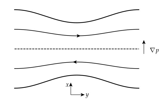
The Hahm–Kulsrud–Taylor (HKT) problem, illustrated in Fig. 1, has a magnetized plasma enclosed by two conducting walls in slab geometry. Before the conducting walls are perturbed, the initial magnetic field is a smooth function of space in the domain with and . The in-plane component points in the direction with ; together with a non-uniform component and the pressure , the system is in force balance; i.e., the equation
| (10) |
is satisfied. Assuming a periodic boundary condition along the direction, we then impose a sinusoidal perturbation with an up-down symmetry that displaces the conducting walls at to , where is the wavenumber. As the system evolves to a new equilibrium subject to the ideal MHD constraint, current singularities, including a Dirac -function current sheet and a pressure-gradient-driven current singularity, will develop at and around the resonant surface (the dashed line in Figure 1).
In response to the boundary perturbation, the flux surfaces adjust their geometries while preserving the magnetic fluxes between them in accordance with the ideal MHD constraints. The new MHD equilibrium satisfies the Grad–Shafranov equation in Cartesian geometry
| (11) |
where
| (12) |
Here, the magnetic field in Cartesian geometry, with being the direction of translational symmetry, is expressed in terms of the poloidal (in-plane) flux function as
| (13) |
In an equilibrium state, both the out-of-plane component and the plasma pressure are functions of .
Because the magnetic fluxes are conserved, the magnetic field is determined by the geometry of flux surfaces. To describe the geometry of flux surfaces, we first need to choose a variable to label them. Let be the positions of flux surfaces along the direction before the boundary perturbation is imposed. The initial condition yields the poloidal (in-plane) magnetic flux function . While it is customary in toroidal confinement devices to label flux surfaces by the magnetic flux function, for the HKT problem it is convenient to label the flux surfaces with their initial positions because a single value of can correspond to more than one flux surface.
With this labeling, the geometry of flux surfaces is described by a mapping from to via a function . Using the chain rule, we can express the partial derivatives with respect to the Cartesian coordinates in terms of the partial derivatives to the coordinates :
| (14) |
| (15) |
Here, the subscripts of the partial derivatives on the left-hand side indicate the coordinates that are held fixed; the partial derivatives on the right-hand side are with respect to the coordinates. Hereafter, partial derivatives are taken to be with respect to the coordinates by default, unless otherwise indicated by the subscripts.
Using these relations for partial derivatives, the Cartesian components of the in-plane magnetic field are given by
| (16) |
and
| (17) |
The out-of-plane component is determined by the conservation of the out-of-plane magnetic flux as
| (18) |
Here, is the initial -component of the magnetic field and the flux surface average is defined as
| (19) |
for an arbitrary function , where is the period of the system along the direction. Likewise, the pressure is determined by the adiabatic energy equation as
| (20) |
where is the initial pressure profile and is the adiabatic index.
2.2 Outer-Region Solution
For a small boundary perturbation, we may linearize the GS equation in terms of the displacements of the flux surfaces along the direction . To the leading order of , the magnetic field components are
| (24) |
| (25) |
and
| (26) |
The linearized pressure is
| (27) |
Using Eqs. (24–27) and the relation in Eq. (23), the linearized GS equation now reads
| (28) |
If we adopt the ansatz , then and the linearized GS equation reduces to
| (29) |
The general solution of Eq. (29) is a linear superposition of two independent solutions
| (30) |
and the boundary condition requires
| (31) |
The independent solution in Eq. (30) diverges at . If we insist that the linear solution is valid everywhere, then we must set ; the boundary condition (31) then determines the coefficient . However, this solution is not physically tenable. Because , the geometry of the flux surfaces is approximately given by in the vicinity of . Hence, the flux surfaces with overlap, causing a condition that is physically not permitted. We conclude that the linear solution is not valid within an inner region with and a nonlinear solution must be sought.
2.3 Inner-Layer Solution
A general nonlinear solution for the inner layer near a resonant surface was first developed by Rosenbluth, Dagazian, and Rutherford (hereafter RDR) for the bifurcated equilibrium after an ideal internal kink instability [23]. The RDR solution was later adapted to the HKT problem with [17, 18]. Here, we generalize previous approaches to incorporate the pressure-gradient effects.
Because the inner region is a thin layer, we assume the conditions and are satisfied. Under these assumptions, the dominant balance of the GS equation (23) is given by
| (32) |
Integrating Eq. (32) yields
| (33) |
where
| (34) |
and is an arbitrary function that will be determined later by asymptotic matching of the inner-layer solution to the outer-region solution. The factor comes from the requirement that must be satisfied to avoid overlapping flux surfaces. Without loss of generality, we are free to set , and the tangential discontinuity of at is then given by
| (35) |
This tangential discontinuity corresponds to a Dirac -function singularity in the current density.
Using the flux function for the HKT problem and integrating Eq. (33) again yields the inner-layer solution of RDR
| (36) |
where the function , which describes the geometry of the resonant surface, is yet to be determined.
2.4 Incompressibility Constraint
The functions and are not independent, but are implicitly related through Eq. (34) as we will see below. First, we determine and in the inner layer by substituting for in Eqs. (18) and (20). Then, applying the obtained and in Eq. (34), the resulting relation
| (37) | |||||
gives a relation between and .
We now show that Eq. (37) is approximately equivalent to the incompressible constraint in the strong-guide-field limit with . From Eq. (37), the differentials and are related by
| (38) | |||||
where we have used the relation to eliminate . In the strong-guide-field limit, the first term in the right-hand side of Eq. (38) is the dominant term. As the leading order approximation, we may ignore other terms in the equation, resulting in the relation
| (39) |
Integrating Eq. yields
| (40) |
where is a constant. Finally, we apply Eq. (40) in Eq. (36) and obtain
| (41) |
Equation (41) has a simple physical meaning: The plasma in the inner layer is uniformly compressed or expanded, and the constant is the compression ratio. Because the inner-layer solution is to be matched to the outer-region solution and the latter is not compressive (up to the linear approximation), the compression ratio must assume the value ; that is, the plasma approximately satisfies the incompressibility constraint. It should be noted, however, that the incompressibility constraint will not be valid if the boundary perturbation has an Fourier component. In this case, the constant needs to be determined by the asymptotic matching as well.
2.5 Asymptotic Matching
The inner-layer solution must be asymptotically matched with the outer-region solution to have a complete solution. For simplicity, we will assume the strong-guide-field limit and replace the relation (37) by the incompressibility constraint
| (42) |
In this limit, to the leading order approximation, the effect of pressure gradient on the geometry of flux surfaces is negligible. Moreover, because the pressure gradient also does not affect the outer-region solution, the asymptotic matching procedure, which we will outline below, is identical to that for the case with [17].
The outer-region solution is expressed in terms of the displacements of flux surfaces. Therefore, to facilitate the matching, we express the flux surface displacement of the inner-layer solution as
| (43) |
and examine its asymptotic behavior as .
From the incompressibility constraint (42), we can infer that as . Hence, in the asymptotic limit of we can split the integral in Eq. (43) into two parts, yielding
| (44) | |||||
This asymptotic behavior of the inner-layer solution as should match the behavior of the outer-region solution in the limit of , which is
| (45) |
Matching Eqs. (44) and (45) yields and the following two conditions:
| (46) |
and
| (47) |
Here, we use the notation in the second condition because, as we will see later, Eq. (47) can not be matched exactly.
The matching condition (46) gives an integral equation to determine the function as follows: by eliminating in favor of using the incompressibility constraint (42) in Eq. (46), we obtain
| (48) |
However, analytically solving this equation to obtain is a daunting task. By studying the behavior of around and , RDR suggested a function form as an approximate solution. This suggestion was confirmed by Loizu and Helander with a numerical solution of the integral equation [24]. Moreover, by fitting the function form with the numerical solution, they also determined the coefficient in front, yielding
| (49) |
Next, for the matching condition (47), it is clear that cannot be matched with exactly. Following RDR, we expand as a Fourier series
| (50) |
and only match the term; that gives
| (51) |
Finally, we use the relation (51) to eliminate in the boundary condition (31), yielding an equation for :
| (52) |
The solution is
| (53) |
Here, the sign for the square root in Eq. (53) is chosen such that in the limit of a small perturbation.
Now, we have obtained , , , and . We can then solve Eq. (42) to obtain , which completes the necessary information to calculate the RDR solution, Eq. (36). Solving from Eq. (42) in general requires a numerical treatment. However, the leading order behavior of in the limit of can be obtained analytically as [18]
| (54) |
where the coefficient can be expressed in terms of the gamma function [25] as
| (55) |
2.6 Pressure-Gradient-Driven Current Singularity
Our analysis thus far has shown that the effect of pressure gradient on the geometry of flux surfaces is negligible. We are now in a position to discuss the effect of pressure gradient on the current density distribution. We are primarily interested in the current density in the vicinity of the resonant surface, i.e., the inner-layer solution.
In the strong-guide-field limit, the plasma is approximately incompressible; therefore, from Eqs. (18) and (20) we have and as the leading order approximation. To calculate the current density requires , but we cannot simply assume for the following reason: when the guide field is strong, both and are close to constant, with different small variations to account for the force balance under different conditions, and these differing small variations give rise to different derivatives for the two fields. To obtain an approximation for , we take the derivative of Eq. (34) with respect to , yielding
| (56) |
Hence,
| (57) |
Using Eq. (57) in Eq. (22) we can obtain the poloidal current density
| (58) |
In the vicinity of , and . Assuming , the pressure gradient term dominates and the poloidal current density diverges as .
Next, we calculate the the out-of-plane current density . The dominant component of is . Therefore, the out-of-plane current density
| (59) |
which is not affected by the pressure. Using the asymptotic behavior (54), the leading order behavior of near is
| (60) |
Hence, the out-of-plane component as .
Now, we put our results in the context of the conventional treatment of the Pfirsch–Schlüter current density. For a solution of the GS equation, the perpendicular component of the current density is
| (61) | |||||
and the divergence of is
| (62) | |||||
Here, we have used that is the direction of symmetry and that both and are flux functions.
The parallel current density is given by
| (63) | |||||
Here, in the last step we have applied the GS equation (11). From Eqs. (62) and (63), we see that the magnetic differential equation (4) is indeed satisfied:
| (64) |
For the HKT problem, the parallel and the perpendicular components of the current density can be obtained from Eqs. (63) and (61) as
| (65) |
and
| (66) |
Alternatively, we can also obtain and from Eqs. (58) and (59) by making appropriate projections. Note that and ; therefore, in the strong-guide-field limit the perpendicular component dominates.
Equations (65) and (66) show that the Pfirsch–Schlüter current density and the diamagnetic current density both diverge as . If we assume that the system size along the direction is the same as the size along the direction, the equivalent “rotational” transform is given by
| (67) |
Now, if we use the symbol to represent the rotational transform for the time being, the Pfirsch–Schlüter current density does have a -type singularity; however, the underlying reason for its divergence is not what is commonly assumed.
In the conventional picture, the -type singularity arises because the magnetic differential operator is thought to become non-invertible at rational surfaces, as suggested by the expressions (4) and (8) using a straight-field-line coordinate system. It is commonly assumed that and the straight-field-line coordinate system are well-behaved; therefore, the -type singularity follows from Eq. (9). In contrast, our results show that the diamagnetic current density diverges as and likewise, from Eq. (62), that diverges as as well. A crucial point is that because of the formation of the Dirac -function current singularity, the poloidal magnetic field does not go to zero as at the resonant surface; instead, as . Consequently, the magnetic differential operator is invertible, and the magnetic differential equation (4) implies that the parallel current density diverges in the same way as .111Strictly speaking, it may be more appropriate to describe the operator as conditionally invertible at . Because the function goes to zero at and , the equation is solvable only when approaches zero sufficiently fast as approaches and such that the function is integrable. This condition is satisfied for on the right-hand side of the magnetic differential equation (4).
How do we reconcile the fact that the operator is invertible at the resonant surface with its non-invertible appearance in a straight-field-line coordinate system? To answer this question, it is instructive to construct such a coordinate system. Because the initial magnetic field lines are straight, the Cartesian coordinates are a straight-field-line coordinate system. Now, if we take a Lagrangian perspective by describing the final state in terms of the mapping from the initial positions of fluid elements to their final positions , the initial coordinates are also a straight-field-line coordinate system for the final state due to the ideal MHD frozen-in constraint. In the Lagrangian perspective, the magnetic field at is determined by the initial magnetic field at and the mapping via the relation [26, 20]
| (68) |
where is the Jacobian of the mapping.
Although our GS formulation is not fully Lagrangian, we can reconstruct the Lagrangian mapping of fluid elements from the initial to the final state once the solution is obtained. In this 2D problem, the fluid motion is limited to an - plane. So, the coordinates of the initial and final states are identical, . In an - plane, for each fluid element labeled by in the final state, we need to find its initial position . This “inverse” Lagrangian mapping can be expressed as a function . From the conservation of magnetic flux through an infinitesimal fluid element
| (69) |
and using Eq. (18) to relate and , we can calculate
| (70) |
and integrate it along each constant- contour to obtain . Using the RDR solution (36) in Eq. (70) yields
| (71) |
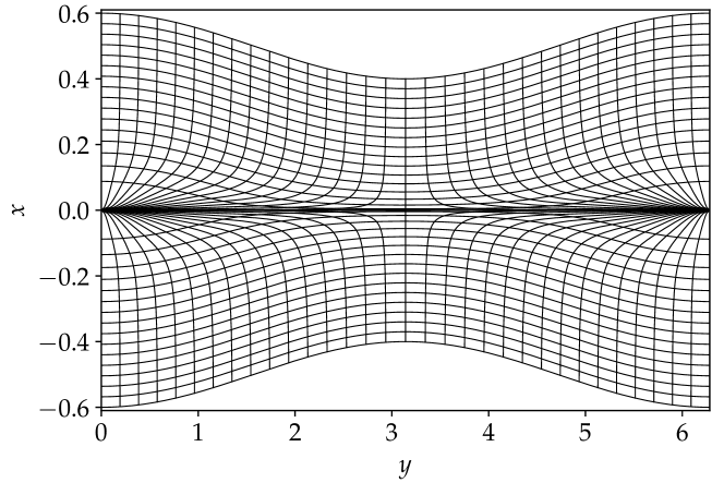
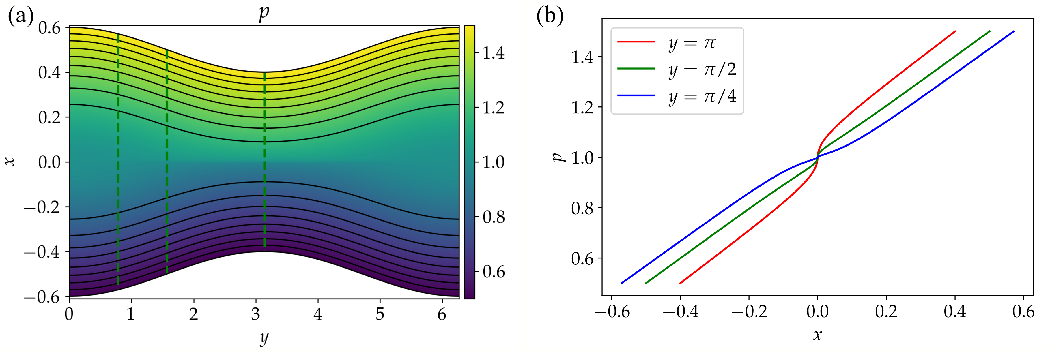
In the limit of , everywhere except at and , where diverges as . Therefore, the straight-field-line coordinate system becomes ill-behaved at the resonant surface, and that explains why the invertible operator appears to be non-invertible in such a coordinate system. Figure 2 shows a constant- slice of the straight-field-line coordinate for the HKT problem with , , and , where the solid lines are constant- or constant- coordinate curves. The singular nature of the coordinate system at the resonant surface is evident, as all the constant- coordinate curves converge towards or .
Now, the critical question is: Does the -type current singularity lead to an infinite current? Fortunately, the answer is no, and the reason can be attributed to the Dirac -function singularity that simultaneously appears at the resonant surface. The finite tangential discontinuity , where denotes the jump across an interface, arises from a continuous initial magnetic field through squeezing the space between flux surfaces [16]. As we can infer from the RDR solution (36), for flux surfaces sufficiently close to the resonant surface such that the condition
| (72) |
is satisfied, the mapping from the flux surface label to the physical distance is quadratic:
| (73) |
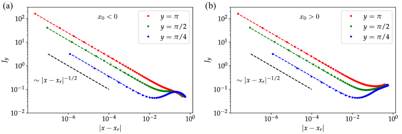
Because and , where , the condition (72) eventually will be satisfied with a sufficiently small for all except at and . As such, the mapping eventually will become quadratic, , although the transition to the quadratic mapping will occur at different for different . Because of the quadratic mapping, the poloidal current density becomes . And since is integrable, the total current does not diverge.
What about at and where the mapping is not quadratic? Because at those locations and , Eqs. (58) gives , which does not diverge. Moreover, to compensate for the strong squeezing of the quadratic mapping, the flux surfaces in the downstream regions near and have to bulge out. Consequently, the scaling at and becomes ; see Ref. [18].
Intuitively, the scaling can be understood as follows. The quadratic mapping causes a steepening of the pressure gradient:
| (74) |
Because the pressure gradient is balanced by the force for an MHD equilibrium, the perpendicular current density , and diverges in the same manner. Finally, the parallel current density satisfies the magnetic differential equation (4), and the operator is invertible; therefore, as well.
3 Numerical Verification of the Analytic Solutions
We now compare the analytic solutions in Section 2 with numerical solutions using a GS solver. The GS solver has been extensively tested, showing good agreement with the solutions of a fully Lagrangian solver [16] and the SPEC code [18] for the HKT problem with . Here, we consider an initial equilibrium with a linear pressure profile
| (75) |
and a magnetic field
| (76) |
The parameters in the following numerical calculations are: the domain sizes and ; the guide field ; the mean pressure ; the pressure gradient ; the perturbation amplitude ; the adiabatic index .
In our previous studies, we assumed a mirror symmetry across the mid-plane and only solved the GS equation in half of the domain with . In this study, because of the asymmetric pressure profile across the resonant surface, we cannot impose the mirror symmetry. We divide the domain into two regions separated by the flux surface labeled by and solve the GS equation in each region by a descent method. Simultaneously with the iteration in both regions, the flux surface is allowed to move until the force-balance condition is satisfied.
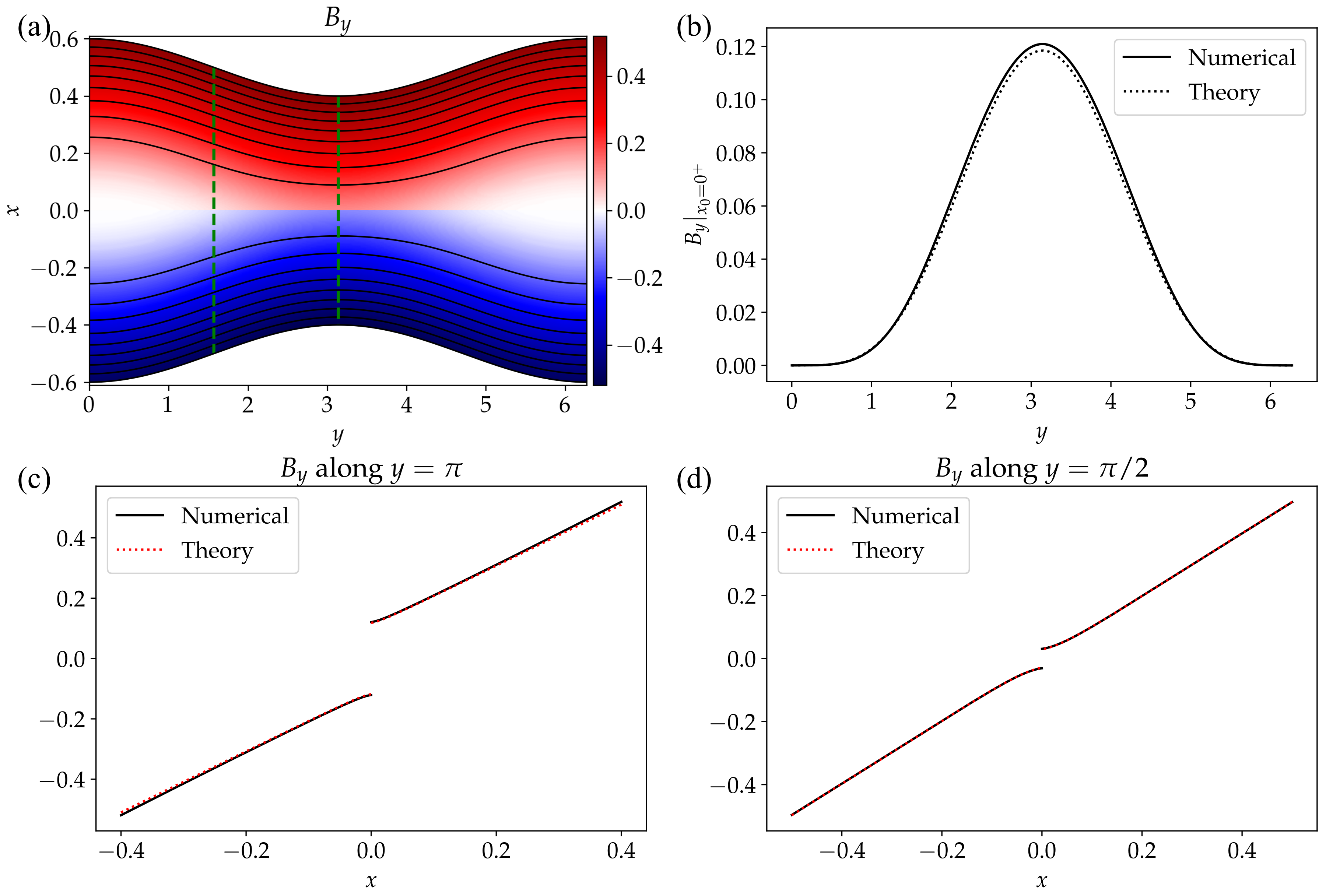
Panel (a) of Figure 3 shows a numerical solution of the component in the entire domain. Panels (b–d) show a few selected one-dimensional (1D) cuts of the numerical solution, together with the corresponding analytical solution (33). The analytic and the numerical solutions are in good agreement. The magnetic field is discontinuous across the resonant surface, corresponding to a Dirac -function current singularity.
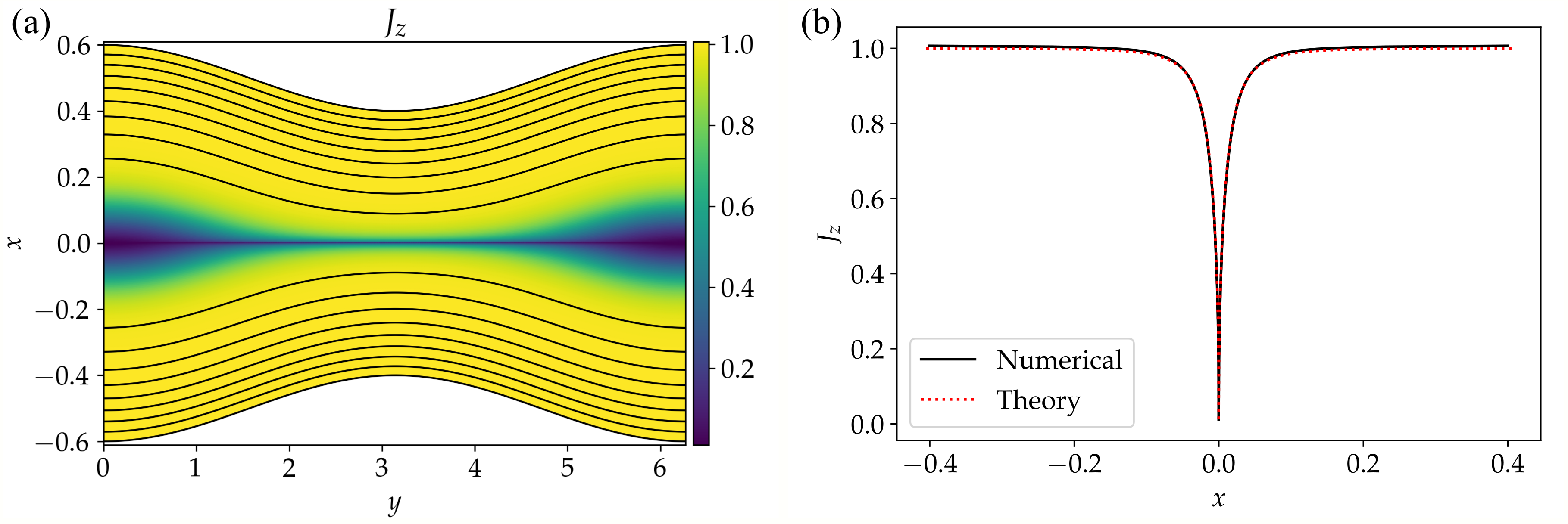
Figure 4 compares the numerical solution of the component with the theoretical prediction using Eq. (59). Here, at the resonant surface as the theory predicts. Likewise, Figure 5 shows comparisons between the numerical solutions of along selected 1D cuts and the theoretical predictions using Eq. (58). In this figure, the horizontal axis is the distance between the flux surface at and the resonant surface at . As predicted by the theory, diverges as near the resonant surface.
Finally, Figure 6 shows a numerical solution of the pressure in the entire domain and along selected 1D cuts. Here, the steepening of the pressure gradient due to the squeezing of flux surfaces near the resonant surface is evident. Examining the solutions in the vicinity of the resonant surface indicates that the , as expected from our analysis.
As a remark, although the analytic theory is derived under the strong-guide-field limit, we find that the theoretical predictions remain close to numerical results even for a moderate guide field such as .
4 Discussions and Conclusion
In summary, we have derived an analytic theory for the pressure-gradient-driven current singularity near the resonant surface of the ideal Hahm–Kulsrud–Taylor (HKT) problem and have validated the theory with numerical solutions. Our key finding is that although the current density diverges as , where is the difference of the rotational transform relative to the resonant surface, this singularity does not lead to a divergent total current. The reason is that the distance between the resonant surface and an adjacent flux surface is not proportional to . Because of the formation of a Dirac -function current sheet at the resonant surface, the neighboring flux surfaces are strongly packed, and the distance . Consequently, the current density , which is integrable and the total current is finite.
Our analysis also finds that the Pfirsh–Schlüter current density and the diamagnetic current density both diverge as , where the diamagnetic current density is the dominant component. The diamagnetic current density diverges because the strong packing of flux surfaces near the resonant surface causes a steepening of the pressure gradient; therefore, . Furthermore, solving the magnetic differential equation (4) yields the parallel current density diverging in the same manner as the perpendicular component . Notably, contrary to the conventional wisdom that the pressure needs to flatten at rational surfaces to have an integrable current density, here we show that the current singularity remains integrable despite a steepening of the pressure gradient.
Our analysis assumes that the initial pressure gradient does not diverge and is non-vanishing at . More generally, we may consider an initial condition with , where such that the current density is integrable. After the boundary perturbation, the current density . Because the power index if , the current density is integrable. Furthermore, we may consider an initial magnetic field . After the boundary perturbation, the formation of a Dirac -function current sheet requires the distance between flux surfaces to scale as ; consequently, the current density , which is integrable. In all these cases, as long as the initial current density is integrable, the current density in the perturbed state is also integrable.
Although our conclusion is obtained with a simple prototype problem, a similar conclusion probably applies to more general magnetic fields and potentially resolves the paradox of non-integrability of the Pfirsch–Schlüter current density. If that is to be the case, then a weak (i.e., non-smooth) ideal MHD equilibrium solution with a continuum of nested flux surfaces, a continuous pressure distribution with non-vanishing pressure gradients on rational surfaces, and a continuous rotational transform is not prohibited. Such an equilibrium may be pathological, to quote Grad, but nonetheless mathematically intriguing to contemplate.
References
- [1] Lyman Spitzer. The stellarator concept. Physics of Fluids, 1(4):253, 1958.
- [2] Allen H. Boozer. What is a stellarator. Phys. Plasmas, 54(5):1647–1655, 1998.
- [3] Per Helander. Theory of plasma confinement in non-axisymmetric magnetic fields. Reports on Progress in Physics, 77(8):087001, jul 2014.
- [4] Allen H. Boozer. Stellarator design. Journal of Plasma Physics, 81(06), dec 2015.
- [5] S. P. Hirshman and J. C. Whitson. Steepest-descent moment method for three-dimensional magnetohydrodynamic equilibria. Physics of Fluids, 26(12):3553, 1983.
- [6] Mark Taylor. A high performance spectral code for nonlinear MHD stability. Journal of Computational Physics, 110(2):407–418, feb 1994.
- [7] P. R. Garabedian. Three-dimensional stellarator codes. Proceedings of the National Academy of Sciences, 99(16):10257–10259, jul 2002.
- [8] D. W. Dudt and E. Kolemen. DESC: A stellarator equilibrium solver. Physics of Plasmas, 27(10):102513, oct 2020.
- [9] John R. Cary and M. Kotschenreuther. Pressure induced islands in three-dimensional toroidal plasma. Physics of Fluids, 28(5):1392, 1985.
- [10] Chris C. Hegna and A. Bhattacharjee. Magnetic island formation in three-dimensional plasma equilibria. Physics of Fluids B: Plasma Physics, 1(2):392–397, feb 1989.
- [11] Harold Grad. Toroidal containment of a plasma. Phys. Fluids, 10(1):137–154, 1967.
- [12] S. R. Hudson and B. F. Kraus. Three-dimensional magnetohydrodynamic equilibria with continuous magnetic fields. Journal of Plasma Physics, 83(04), jul 2017.
- [13] B. F. Kraus and S. R. Hudson. Theory and discretization of ideal magnetohydrodynamic equilibria with fractal pressure profiles. Physics of Plasmas, 24(9):092519, sep 2017.
- [14] T. S. Hahm and R. M. Kulsrud. Forced magnetic reconnection. Phys. Fluids, 28(8):2412–2418, 1985.
- [15] R. L. Dewar, A. Bhattacharjee, R. M. Kulsrud, and A. M. Wright. Plasmoid solutions of the hahm-kulsrud-taylor equilibrium model. Phys. Plasmas, 20:082103, 2013.
- [16] Yao Zhou, Yi-Min Huang, Hong Qin, and A. Bhattacharjee. Formation of current singularity in a topologically constrained plasma. Phys. Rev. E, 93:023205, 2016.
- [17] Yao Zhou, Yi-Min Huang, A. H. Reiman, Hong Qin, and A. Bhattacharjee. Magnetohydrodynamical equilibria with current singularities and continuous rotational transform. Physics of Plasmas, 26(2):022103, feb 2019.
- [18] Yi-Min Huang, Stuart R. Hudson, Joaquim Loizu, Yao Zhou, and Amitava Bhattacharjee. Numerical study of -function current sheets arising from resonant magnetic perturbations. Physics of Plasmas, 29(3):032513, 2022.
- [19] Yi-Min Huang, A. Bhattacharjee, and Ellen G. Zweibel. Do potential fields develop current sheets under simple compression or expansion? Astrophys. J. Lett., 699:L144–L147, 2009.
- [20] Yao Zhou, Hong Qin, J. W. Burby, and A. Bhattacharjee. Variational integration for ideal magnetohydrodynamics with built-in advection equations. Phys. Plasmas, 21:102109, 2014.
- [21] S. R. Hudson, R. L. Dewar, G. Dennis, M. J. Hole, M. McGann, G. von Nessi, and S. Lazerson. Computation of multi-region relaxed magnetohydrodynamic equilibria. Physics of Plasmas, 19(11):112502, nov 2012.
- [22] Yao Zhou, Yi-Min Huang, Hong Qin, and A. Bhattacharjee. Constructing current singularity in a 3d line-tied plasma. Astrophys. J., 852:3, 2018.
- [23] M. N. Rosenbluth, R. Y. Dagazian, and P. H. Rutherford. Nonlinear properties of the internal m=1 kink instability in the cylindrical tokamak. Phys. Fluids, 16(11):1894–1902, 1973.
- [24] J. Loizu and P. Helander. Unified nonlinear theory of spontaneous and forced helical resonant MHD states. Phys. Plasmas, 24(4):040701, 2017.
- [25] Milton Abramowitz and Irene A. Stegun, editors. Handbook of Mathematical Functions with Formulas, Graphs, and Mathematical Tables. National Bureau of Standards, 10th printing, with corrections edition, 1972.
- [26] William A. Newcomb. Lagrangian and Hamiltonian Methods in Magnetohydrodynamics. Nuclear Fusion Supplement, Part 2, pages 451–463, 1962.