In- and out-of-equilibrium ab initio theory of electrons and phonons

Abstract

In this work we lay down the ab initio many-body quantum theory of electrons and phonons in- and out-of-equilibrium at any temperature. Our focus is on the harmonic approximation but the developed tools clearly indicate how to incorporate anharmonic effects. We begin by addressing a fundamental issue concerning the ab initio Hamiltonian in the harmonic approximation, which we show must be determined self-consistently to avoid inconsistencies. After identifying the most suitable partitioning into a “noninteracting” and an “interacting” part we embark on the Green’s function diagrammatic analysis. We single out key diagrammatic structures to carry on the expansion in terms of dressed propagators and screened interaction. The final outcome is the finite-temperature nonequilibrium extension of the Hedin equations, featuring the appearance of the time-local Ehrenfest diagram in the electronic self-energy. The Hedin equations have limited practical utility for real-time simulations of systems driven out of equilibrium by external fields. To overcome this limitation, we leverage the versatility of diagrammatic expansion to generate a closed system of integro-differential equations for the Green’s functions and nuclear displacements. These are the Kadanoff-Baym equations for electrons and phonons. Another advantage of the diagrammatic derivation is the ability to use conserving approximations, which ensure the satisfaction of the continuity equation and the conservation of total energy during time evolution. As an example we show that the adiabatic Born-Oppenheimer approximation is not conserving whereas its dynamical extension is conserving only provided that the electrons are treated in the Fan-Migdal approximation with a dynamically screened electron-phonon coupling. We also derive the formal solution of the Kadanoff-Baym equations in the long time limit and at the steady state. The expansion of the phononic Green’s function around the quasi-phonon energies points to a possible correlation-induced splitting of the phonon dispersion in materials with no time-reversal invariance.

I Introduction

The concept of phonons as quasi-particles describing independent excitations of the nuclear lattice dates back to almost a century ago Bloch (1929); Frenkel (1932). Nonetheless, the first rigorous theory of electrons and phonons saw the light of day in 1961 Baym (1961). In a seminal paper Baym showed how to map the original electron-nuclear Hamiltonian onto a low-energy or equivalently electron-phonon ($e$-$ph$) Hamiltonian, and derived a set of equations for the electronic and phononic Green’s functions (GF) $G$ and $D$. The Baym equation for the electronic GF was rather implicit though. In the mid-sixties Hedin used the same technique as Baym, the so called source-field method or field-theoretic approach, to generate a more explicit set of equations for the electronic GF at clamped nuclei Hedin (1965). The contributions by Baym and Hedin have been largely ignored by the electron-phonon community (including ourselves) in favor of semi-empirical Hamiltonians. Only recently the works of Baym, Hedin and a few others Keating (1968); van Leeuwen (2004); Marini et al. (2015) have been rigorously merged by Giustino in a unified many-body GF framework Giustino (2017), which we keep naming the Hedin-Baym equations (instead of “Hedin equations”) after Giustino.

Despite these recent notable advances the formal theory of electrons and phonons is still not complete. We stress here the word “formal” as this paper does not address specific aspects or computational strategies related to the $e$-$ph$ interaction, for which we refer the reader to excellent textbooks Ziman (1960); Grimvall (1981); Schrieffer (1983); Mahan (2000); Bruus and Flensberg (2004); Giustino (2014); Czycholl (2023) and modern comprehensive reviews Giustino (2017), rather it establishes a mathematically rigorous apparatus for the quantum treatment of electrons and nuclei in the so called harmonic approximation.

Three pivotal issues are still waiting to be clarified and solved. The first issue has to do with the ab initio $e$-$ph$ Hamiltonian, often replaced by semi-empirical Hamiltonians or left unspecified as unnecessary for the implementation of approximate formulas for the phononic dispersions, life-times, etc.. The ab initio $e$-$ph$ Hamiltonian is, however, of paramount relevance. It is necessary for assessing the validity of semi-empirical approaches, for improving approximations based on perturbation theory, for making fair comparisons between different methods and between different approximations within the same method as well as for benchmarking the harmonic approximation against other methods like, e.g., the surface hopping approach Tully (1990) or the exact-factorization scheme Abedi et al. (2010); Requist and Gross (2016). A plausible explanation for the scarce attention given to the ab initio $e$-$ph$ Hamiltonian is that the minimal sensible approximation is nonperturbative. In fact, the ab initio $e$-$ph$ Hamiltonian evaluated at zero $e$-$ph$ coupling does not even contain phonons. A clean derivation of the $e$-$ph$ Hamiltonian can be found in the Baym’s work Baym (1961). However, Baym’s original expression as well as equivalent expressions designed for having a good starting point for perturbative expansions Marini et al. (2015) necessitate the knowledge of the exact equilibrium electronic density $n^{0}$. This means that the ab initio $e$-$ph$ Hamiltonian is unknown unless $n^{0}$ is calculated by other means, e.g., by solving the original electron-nuclear problem. Even assuming that we could find $n^{0}$ somehow, we would still have to face a practical problem. All many-body techniques (including those based on GF) can only be implemented in some approximation, for the exchange-correlation (xc) potential in Density Functional Theory (DFT), for the self-energy in GF theory, for the configuration state functions in the Multi-Configurational Hartree-Fock method, for the intermediate states in the Algebraic Diagrammatic Construction scheme, etc. An approximation in any of the available many-body methods inevitably leads to an inconsistency if the ab initio $e$-$ph$ Hamiltonian is evaluated at the exact $n^{0}$. The inconsistency lies in the fact that the forces acting on the nuclei would not vanish in thermal equilibrium. As we shall see, the ab initio $e$-$ph$ Hamiltonian must be determined self-consistently for it to be used in practice. Such self-consistent concept is completely general, i.e., it is not limited to GF approaches. Of course if an exact method is used than the self-consistent density $n^{0}$ coincides with the exact one.

The second issue is the extension of the Hedin-Baym equations at finite temperature and out-of-equilibrium. This is especially relevant in the light of the overwhelming and steadily increasing number of time-resolved spectroscopy experiments. We mention that at zero-temperature a nonequilibrium Green’s function (NEGF) formulation has been put forward in terms of the nuclear-density correlation function van Leeuwen (2004); Marini and Pavlyukh (2018); Härkönen et al. (2020). We here present the finite-temperature and nonequilibrium extension of the Hedin-Baym equations for the electronic GF and the displacement-displacement correlation function (or phononic GF) Giustino (2017). We anticipate that the main differences are: (i) in all internal vertices the time arguments must be integrated over the $L$-shaped Konstantinov-Perel’s contour Konstantinov and Perel (1961); Wagner (1991); Enz (1992); Stefanucci and Almbladh (2004); Stefanucci and van Leeuwen (2013); (ii) the electronic GF satisfies a Dyson equation with an extra time-local self-energy, whose inclusion is fundamental to recover the Ehrenfest (mixed quantum-classical) dynamics Horsfield et al. (2004a, b); Li et al. (2005); Verdozzi et al. (2006); Galperin et al. (2007, 2008); Dundas et al. (2009); Hussein et al. (2010); Lü et al. (2010); Bode et al. (2011); Hübener et al. (2018). In the context of material science the Ehrenfest self-energy plays a key role in the description of polarons Galperin et al. (2008); Lafuente-Bartolome et al. (2022) and it is expected to be fundamental to detect the phonon-induced coherent modulation of the excitonic resonances Trovatello et al. (2020).

The Hedin-Baym equations have limited practical utility in nonequilibrium problems. Furthermore, the original derivation based on the source-field method allows for solving these equations only iteratively, starting from an approximation to the vertex. The question of whether the iterative procedure converges towards the exact solution is still open. In most applications only one iteration step is performed since the equations resulting from the second interaction are already too complex. All these considerations bring us to the third issue, i.e., how to systematically improve the approximations possibly preserving all fundamental conservation laws. We here present a diagrammatic derivation of the Hedin-Baym equations based on the skeletonic expansion of the electronic and phononic self-energies in terms of interacting electronic and phononic GF and the screened interaction. We highlight three essential merits of the diagrammatic derivation: (i) the possibility of including relevant scattering mechanisms through a proper selection of Feynman diagrams (to be converted into mathematical expressions through the Feynman rules which we provide); (ii) the possibility of using the $\Phi$-derivable criterion Baym (1962) to have a fully conserving dynamics; (iii) the possibility of closing the Kadanoff-Baym equations (KBE) Kadanoff and Baym (1962) through a skeletonic expansion of the self-energies in terms of only interacting GF. The KBE are integro-differential equations for the electronic and phononic NEGF Danielewicz (1984); Stefanucci and van Leeuwen (2013), and they are definitely more practical for investigating the real-time evolution of systems driven out of equilibrium. Furthermore, through the so called Generalized Kadanoff-Baym Ansatz for fermions Lipavský et al. (1986) and bosons Karlsson et al. (2021) the KBE can be mapped onto a much simpler system of ordinary differential equations for a large number of self-energy approximations Schlünzen et al. (2020); Joost et al. (2020); Karlsson et al. (2021); Pavlyukh et al. (2021, 2022a, 2022b); Perfetto et al. (2022).

The paper is organized as follows. In Section II we derive the low-energy Hamiltonian for any system of electrons and nuclei, highlighting its dependence on the equilibrium electronic density and pointing out the necessity of a self-consistent procedure for its determination. In Section III we specialize the discussion to lattice periodic systems, introduce general time-dependent external perturbations and derive the $e$-$ph$ Hamiltonian on the $L$-shaped contour. The equations of motion for the electronic and phononic field operators are derived in Section IV. In Section V we define the many-particle electronic and phononic GF on the contour and construct the Martin-Schwinger hierarchy that these GF satisfy. In Section VI we present the Wick’s theorem as the solution of the noninteracting Martin-Schwinger hierarchy and in Section VII we provide the exact formula of the many-body expansion of the interacting GF in terms of the noninteracting ones. The many-body expansion is mapped onto a diagrammatic theory in Section VIII where we also introduce the notion of self-energies and skeleton diagrams. The skeletonic expansion of the self-energies in terms of the interacting GF and screened Coulomb interaction is shown to lead to the Hedin-Baym equations in Section IX. The Hedin-Baym equations are applicable to systems in- and out-of equilibrium as well as at zero and finite temperature. To study the system evolution or the finite-temperature spectral properties the equations of motion for the GF are more convenient than the Hedin-Baym equations. These equations of motion are derived in Section X. In Section XI we discuss the so called $\Phi$-derivable approximations to the self-energies. The GF satisfying the equations of motion with $\Phi$-derivable self-energies guarantee the fulfillment of all fundamental conservation laws. In Section XII we convert the equations of motion into a coupled system of integro-differential equations for the Keldysh components of the GF; these are the KBE. We first discuss the self-consistent solution of the equilibrium problem and then derive the real-time equations of motion to study the system evolution. We also present the formal solution of the KBE in the long-time limit and for steady-state conditions. The expansion of the phononic GF around the quasi-phonon energies reveals the possibility of a correlation-induced splitting of the phonon dispersion in materials with no time-reversal invariance. The presented formalism can be extended to deal with much more general Hamiltonians than the $e$-$ph$ Hamiltonian. In Section XIII we provide a summary of the main results, illustrate possible extensions and discuss their physical relevance.

II Quantum systems of electrons and nuclei

In this section we lay down a quantum theory of electrons and nuclei which is suited whenever the average nuclear positions remain close to the equilibrium values. Under this “near-equilibrium hypothesis” the nuclei stay away from each other and they can be treated as quantum distinguishable particles. In fact, we can distinguish them by means of techniques like scanning tunneling microscopy or electron diffraction Giustino (2017).

Let $\hat{\psi}({\mathbf{x}}={\mathbf{r}}\sigma)$ be the field operators that annihilate an electron in position ${\mathbf{r}}$ with spin $\sigma$, hence they satisfy the anticommutation relations $\{\hat{\psi}({\mathbf{x}}),\hat{\psi}^{{\dagger}}({\mathbf{x}}^{\prime})\}=\delta_{\sigma\sigma^{\prime}}\delta({\mathbf{r}}-{\mathbf{r}}^{\prime})\equiv\delta({\mathbf{x}}-{\mathbf{x}}^{\prime})$, and $\hat{{\mathbf{R}}}_{i}$, $\hat{{\mathbf{P}}}_{i}$ be the position and momentum operators of the $i$-th nucleus, $i=1,\ldots N_{n}$, satisfying the standard commutation relations $[\hat{R}_{i,\alpha},\hat{P}_{j,\beta}]_{-}=i\delta_{ij}\delta_{\alpha\beta}$, with $\alpha$ and $\beta$ running over the three components of the vectors. The Hamiltonian describing an unperturbed system of electrons interacting with $N_{n}$ nuclei of charge $Z_{i}$ and mass $M_{i}$ reads (we use atomic units throughout the paper)

$$\hat{H}=\hat{H}_{e}+\hat{H}_{n}+\hat{H}_{e-n},$$ (1)

where

$$\hat{H}_{e} =\!\int\!d{\mathbf{x}}\,\hat{\psi}^{{\dagger}}({\mathbf{x}})\Big{[}-\frac{\nabla^{2}}{2}\Big{]}\hat{\psi}({\mathbf{x}}),$$

$$+\frac{1}{2}\!\int\!d{\mathbf{x}}d{\mathbf{x}}^{\prime}\hat{\psi}^{{\dagger}}({\mathbf{x}})\hat{\psi}^{{\dagger}}({\mathbf{x}}^{\prime})v({\mathbf{r}},{\mathbf{r}}^{\prime})\hat{\psi}({\mathbf{x}}^{\prime})\hat{\psi}({\mathbf{x}}),$$ (2)

is the electronic Hamiltonian,

$$\hat{H}_{n}=\sum_{i=1}^{N_{n}}\frac{\hat{P}_{i}^{2}}{2M_{i}}+\frac{1}{2}\sum_{i\neq j}^{N_{n}}Z_{i}Z_{j}v(\hat{{\mathbf{R}}}_{i},\hat{{\mathbf{R}}}_{j}),$$ (3)

is the nuclear Hamiltonian (with $\hat{P}_{i}^{2}=\hat{{\mathbf{P}}}_{i}\cdot\hat{{\mathbf{P}}}_{i}$) and

$$\hat{H}_{e-n}=-\int\!d{\mathbf{x}}\,\hat{n}({\mathbf{x}})\sum_{j=1}^{N_{n}}Z_{j}v({\mathbf{r}},\hat{{\mathbf{R}}}_{j}),$$ (4)

is the electron-nucleus interaction. In Eqs. (2-4) the integral $\int\!d{\mathbf{x}}\equiv\int\!d{\mathbf{r}}\sum_{\sigma}$ signifies a spatial integral and a sum over spin, $v({\mathbf{r}},{\mathbf{r}}^{\prime})=1/|{\mathbf{r}}-{\mathbf{r}}^{\prime}|$ is the Coulomb interaction and $\hat{n}({\mathbf{x}})\equiv\hat{\psi}^{{\dagger}}({\mathbf{x}})\hat{\psi}({\mathbf{x}})$ is the density operator in ${\mathbf{r}}$ for particles of spin $\sigma$. For later purposes we find it convenient to collect all nuclear position and momentum operators into the vectors $\hat{{\mathbf{R}}}=(\hat{{\mathbf{R}}}_{1},\ldots,\hat{{\mathbf{R}}}_{N_{n}})$ and $\hat{{\mathbf{P}}}=(\hat{{\mathbf{P}}}_{1},\ldots,\hat{{\mathbf{P}}}_{N_{n}})$. We also find it useful to define the nuclear potential energy

$$E_{n-n}(\hat{{\mathbf{R}}})\equiv\frac{1}{2}\sum_{i\neq j}^{N_{n}}Z_{i}Z_{j}v(\hat{{\mathbf{R}}}_{i},\hat{{\mathbf{R}}}_{j}),$$ (5)

appearing in Eq. (3), and the electron-nuclear potential

$$V({\mathbf{r}},\hat{{\mathbf{R}}})\equiv\sum_{j=1}^{N_{n}}Z_{j}v({\mathbf{r}},\hat{{\mathbf{R}}}_{j}),$$ (6)

appearing in Eq. (4). The operators of $\hat{H}$ act on the direct-product space $\mathbb{F}\otimes\mathbb{D}_{N_{n}}$ where $\mathbb{F}$ is the electronic Fock space and $\mathbb{D}_{N_{n}}$ is the Hilbert space of the $N_{n}$ distinguishable nuclei.

Expansion around thermal equilibrium.– Consider the interacting system of electrons and nuclei in thermal equilibrium at a certain temperature. Under the “near-equilibrium hypothesis” we can approximate the full Hamiltonian by its second-order Taylor expansion around the equilibrium values of the nuclear positions, which we name ${\mathbf{R}}^{0}=({\mathbf{R}}^{0}_{1},\ldots,{\mathbf{R}}^{0}_{N_{n}})$, and around the equilibrium value of the electronic density, which we name $n^{0}({\mathbf{x}})$. In fact, also the electronic density must stay close to $n^{0}({\mathbf{x}})$ for otherwise the forces acting on the nuclei would be strong enough to drive the nuclei away from ${\mathbf{R}}^{0}$. Notice that ${\mathbf{R}}^{0}$ and $n^{0}({\mathbf{x}})$ do in general depend on the temperature. We also observe that the existence of an inertial reference frame for the coordinates ${\mathbf{R}}^{0}$ is supported by the macroscopic size of the system, i.e., $N_{n}\to\infty$. For finite systems, e.g., molecules or molecular aggregates, the choice of a suitable reference frame is more subtle, see Refs Eckart (1935); Howard and Moss (1970); Wilson et al. (1980); Bunker and Jensen (1998); Sutcliffe (2000); Meyer (2002).

We introduce the displacement (or position fluctuation) operators $\hat{{\mathbf{U}}}_{i}$ and the density fluctuation operator $\Delta\hat{n}$ according to

$$\hat{{\mathbf{U}}}_{i}=\hat{{\mathbf{R}}}_{i}-{\mathbf{R}}^{0}_{i},\quad\quad\quad\quad\Delta\hat{n}({\mathbf{x}})=\hat{n}({\mathbf{x}})-n^{0}({\mathbf{x}}).$$ (7)

In the following we refer to these operators as the fluctuation operators. Formally, the “near-equilibrium hypothesis” is equivalent to restrict full the space $\mathbb{F}\otimes\mathbb{D}_{N_{n}}$ to the subspace of states giving a small average of $\hat{{\mathbf{U}}}_{i}$ and $\Delta\hat{n}$.

The expansion of the nuclear potential energy around the equilibrium nuclear positions yields to second order

$$E_{n-n}(\hat{{\mathbf{R}}})=E_{n-n}({\mathbf{R}}^{0}) +\sum_{i\alpha}\left.\frac{\partial E_{n-n}({\mathbf{R}})}{\partial R_{i,\alpha}}\right|_{{\mathbf{R}}={\mathbf{R}}^{0}}\!\hat{U}_{i,\alpha}$$

$$+\frac{1}{2}\sum_{i\alpha,j\beta}\left.\frac{\partial^{2}E_{n-n}({\mathbf{R}})}{\partial R_{i,\alpha}\partial R_{j,\beta}}\right|_{{\mathbf{R}}={\mathbf{R}}^{0}}\!\hat{U}_{i,\alpha}\hat{U}_{j,\beta}.$$ (8)

In the first term we recognize the electrostatic energy of a nuclear geometry ${\mathbf{R}}^{0}$. As this term is only responsible for an overall energy shift we do not include it in the following discussion. Similarly, the expansion of the electron-nuclear potential yields to second order

$$V({\mathbf{r}},\hat{{\mathbf{R}}})=V({\mathbf{r}})+\sum_{i\alpha}g_{i,\alpha}({\mathbf{r}})\,\hat{U}_{i,\alpha}+\frac{1}{2}\sum_{i\alpha,j\beta}g^{\rm DW}_{i,\alpha;j,\beta}({\mathbf{r}})\,\hat{U}_{i,\alpha}\hat{U}_{j,\beta},$$ (9)

where we define

$$V({\mathbf{r}}) \equiv V({\mathbf{r}},{\mathbf{R}}^{0}),$$ (10a)

$$g_{i,\alpha}({\mathbf{r}}) \equiv\left.\frac{\partial V({\mathbf{r}},{\mathbf{R}})}{\partial R_{i,\alpha}}\right|_{{\mathbf{R}}={\mathbf{R}}^{0}}=-Z_{i}\frac{\partial}{\partial r_{\alpha}}v({\mathbf{r}},{\mathbf{R}}^{0}_{i}),$$ (10b)

$$g^{\rm DW}_{i,\alpha;j,\beta}({\mathbf{r}}) \equiv\left.\frac{\partial^{2}V({\mathbf{r}},{\mathbf{R}})}{\partial R_{i,\alpha}\partial R_{j,\beta}}\right|_{{\mathbf{R}}={\mathbf{R}}^{0}}=\delta_{ij}Z_{i}\frac{\partial^{2}}{\partial r_{\alpha}\partial r_{\beta}}v({\mathbf{r}},{\mathbf{R}}^{0}_{i}).$$ (10c)

Inserting Eq. (9) into Eq. (4) we see that the first term gives rise to a purely electronic operator; it is the potential energy operator for electrons in the classical field generated by a nuclear geometry ${\mathbf{R}}^{0}$. The second and third terms emerge when relaxing the infinite-mass approximation for the nuclei. The third term of Eq. (9) is already quadratic in the displacements and it can therefore be multiplied by the equilibrium density, i.e., $\hat{n}\to n^{0}$ Baym (1961). Going beyond the quadratic (or harmonic) approximation the replacement $\hat{n}\to n^{0}$ is no longer justified; in this case the third term gives rise to the so called Debye-Waller (DW) interaction Allen and Heine (1976).

The low-energy Hamiltonian.– Inserting the expansion of $E_{n-n}$ and $V$ into Eqs. (3) and (4) the total Hamiltonian becomes

$$\hat{H}=\hat{H}_{0,e}+\hat{H}_{0,ph}+\hat{H}_{e-e}+\hat{H}^{\prime}.$$ (11)

The first two terms describe an uncoupled system of noninteracting electrons and $N_{n}$ interacting nuclei in the electric field generated by a frozen electronic density $n^{0}({\mathbf{r}})$

$$\hat{H}_{0,e}=\!\int\!d{\mathbf{x}}\,\hat{\psi}^{{\dagger}}({\mathbf{x}})\Big{[}-\frac{\nabla^{2}}{2}+V({\mathbf{r}})\Big{]}\hat{\psi}({\mathbf{x}}),$$ (12)

$$\hat{H}_{0,ph}=\sum_{i=1}^{N_{n}}\frac{\hat{P}_{i}^{2}}{2M_{i}}+\frac{1}{2}\sum_{i\alpha,j\beta}\hat{U}_{i,\alpha}K_{i,\alpha;j,\beta}\,\hat{U}_{j,\beta},$$ (13)

where we define the elastic tensor

$$K_{i,\alpha;j,\beta}\equiv\left.\frac{\partial^{2}E_{n-n}({\mathbf{R}})}{\partial R_{i,\alpha}\partial R_{j,\beta}}\right|_{{\mathbf{R}}={\mathbf{R}}^{0}}-\int d{\mathbf{x}}\,n^{0}({\mathbf{x}})g^{\rm DW}_{i,\alpha;j,\beta}({\mathbf{r}}),$$ (14)

which is real and symmetric under the exchange $(i,\alpha)\leftrightarrow(j,\beta)$. Already at this stage of the presentation a remark is due. The eigenvalues $\omega^{2}_{\lambda}$ of the tensor $\overline{K}_{i,\alpha;j,\beta}\equiv K_{i,\alpha;j,\beta}/\sqrt{M_{i}M_{j}}$ are not physical and can even be negative such that $\hat{H}_{0,ph}$ does not have a proper ground state. It is therefore generally not possible to define annihilation and creation operators $\hat{b}_{\lambda}$ and $\hat{b}^{{\dagger}}_{\lambda}$ to rewrite Eq. (13) in the form $\hat{H}_{0,ph}=\sum_{\lambda}\omega_{\lambda}(\hat{b}^{{\dagger}}_{\lambda}\hat{b}_{\lambda}+\frac{1}{2})$. The ab initio low-energy Hamiltonian evaluated at vanishing coupling $g_{i,\alpha}$ [hence $\hat{H}^{\prime}=0$, see Eq. (21)] does not contain physical quanta of vibrations (phonons in solids). These excitations can only emerge from a proper nonperturbative treatment, see Section XII.1.

The third term in Eq. (11) is the electron-electron ($e$-$e$) interaction Hamiltonian

$$\hat{H}_{e-e}=\frac{1}{2}\!\int\!d{\mathbf{x}}d{\mathbf{x}}^{\prime}\hat{\psi}^{{\dagger}}({\mathbf{x}})\hat{\psi}^{{\dagger}}({\mathbf{x}}^{\prime})v({\mathbf{r}},{\mathbf{r}}^{\prime})\hat{\psi}({\mathbf{x}}^{\prime})\hat{\psi}({\mathbf{x}}),$$ (15)

while the last term is the contribution linear in the nuclear displacements

$$\hat{H}^{\prime}=\sum_{i\alpha}\left[\left.\frac{\partial E_{n-n}({\mathbf{R}})}{\partial R_{i,\alpha}}\right|_{{\mathbf{R}}={\mathbf{R}}^{0}}-\int\!d{\mathbf{x}}\;g_{i,\alpha}({\mathbf{r}})\hat{n}({\mathbf{x}})\right]\hat{U}_{i,\alpha}.$$ (16)

The Hamiltonian in Eq. (11) with the four contributions as in Eqs. (12), (13), (15) and (16) is identical to that of Ref. Baym (1961). We here make a step further. Although it is not evident the operator $\hat{H}^{\prime}$ is quadratic in the fluctuation operators. To show it we consider the Heisenberg equation of motion for the time-dependent average of the nuclear momentum operators. Let $\hat{\mbox{$\mathcal{U}$}}(t,t_{0})$ be the evolution operator from some initial time $t_{0}$ to time $t>t_{0}$ and $\hat{\mbox{$\mathcal{U}$}}(t_{0},t)=[\hat{\mbox{$\mathcal{U}$}}(t,t_{0})]^{{\dagger}}$. Henceforth any operator $\hat{O}(t)$ in the Heisenberg picture carries a subscript “$H$”, i.e., $\hat{O}_{H}(t)=\hat{\mbox{$\mathcal{U}$}}(t_{0},t)\hat{O}(t)\hat{\mbox{$\mathcal{U}$}}(t,t_{0})$. The time-dependent average $O(t)$ of the operator $\hat{O}(t)$ is defined according to

$$O(t)={\rm Tr}[\hat{\rho}\,\hat{O}_{H}(t)],$$ (17)

where

$$\hat{\rho}=\frac{e^{-\beta(\hat{H}-\mu\hat{N}_{e})}}{{\rm Tr}[e^{-\beta(\hat{H}-\mu\hat{N}_{e})}]}$$ (18)

is the thermal density matrix, with $\beta$ the inverse temperature, $\mu$ the chemical potential and $\hat{N}_{e}=\int d{\mathbf{x}}\,\hat{n}({\mathbf{x}})$ the operator for the total number of electrons. Using $i\frac{d}{dt}\hat{O}_{H}(t)=[\hat{O}_{H}(t),\hat{H}_{H}(t)]$ we find

$$\frac{dP_{i,\alpha}(t)}{dt} =-\left.\frac{\partial E_{n-n}({\mathbf{R}})}{\partial R_{i,\alpha}}\right|_{{\mathbf{R}}={\mathbf{R}}^{0}}+\int\!d{\mathbf{x}}\;g_{i,\alpha}({\mathbf{r}})n({\mathbf{x}},t)$$

$$-\sum_{j\beta}K_{i,\alpha;j,\beta}U_{j,\beta}(t),$$ (19)

where $n({\mathbf{x}},t)$ and $U_{j,\beta}(t)$ are the time-dependent averages of the electronic density $\hat{n}({\mathbf{r}})$ and nuclear displacement $\hat{U}_{j,\beta}$. In thermal equilibrium the l.h.s. vanishes, $n({\mathbf{x}},t)=n^{0}({\mathbf{x}})$ and $U_{j,\beta}=0$. Therefore

$$\left.\frac{\partial E_{n-n}({\mathbf{R}})}{\partial R_{i,\alpha}}\right|_{{\mathbf{R}}={\mathbf{R}}^{0}}=\int\!d{\mathbf{x}}\;g_{i,\alpha}({\mathbf{r}})n^{0}({\mathbf{x}}),$$ (20)

according to which we can rewrite Eq. (16) as

$$\hat{H}^{\prime}=-\sum_{i\alpha}\int d{\mathbf{x}}\;g_{i,\alpha}({\mathbf{r}})\Delta\hat{n}({\mathbf{x}})\,\hat{U}_{i,\alpha},$$ (21)

where $\Delta\hat{n}({\mathbf{r}})$ is the density fluctuation operator defined in Eq. (7). In this form $\hat{H}^{\prime}$ is manifestly quadratic in the fluctuation operators.

Inserting Eq. (20) in Eq. (19) we also see that the equation of motion for the momentum operators simplifies to

$$\frac{dP_{i,\alpha}(t)}{dt}=\int\!d{\mathbf{x}}\;g_{i,\alpha}({\mathbf{r}})\Delta n({\mathbf{x}},t)-\sum_{j\beta}K_{i,\alpha;j,\beta}U_{j,\beta}(t).$$ (22)

We can interpret the elastic tensor $K$ as the nuclear-force tensor of a system with frozen electronic density, i.e., with $\Delta n({\mathbf{x}},t)=0$, or alternatively with vanishing coupling $g_{i,\alpha}$. In general $g_{i,\alpha}\neq 0$ and out of equilibrium $\Delta n({\mathbf{x}},t)\neq 0$, and the first term in Eq. (22) significantly contributes to the nuclear forces.

The Hamiltonian in Eq. (11) is the low-energy approximation of the full Hamiltonian in Eq. (1). The expansion around the equilibrium nuclear geometry and around the equilibrium density has inevitably made Eq. (11) to depend on these quantities. The scalar potential $V$ and the electron-nuclear coupling $g$ are determined from the sole knowledge of the equilibrium positions ${\mathbf{R}}^{0}$ whereas the elastic tensor $K$ depends on both ${\mathbf{R}}^{0}$ and $n^{0}$, see Eq. (14). Notice that the dependence of $\hat{H}$ on $n^{0}$ is through $K$ as well as $\Delta\hat{n}$, see Eq. (21). In the following we assume that ${\mathbf{R}}^{0}$ is known and therefore that $V$ and $g$ are given. Strategies to obtain good approximations to the equilibrium nuclear geometry are indeed available, e.g., the Born-Oppenheimer approximation, see also discussion in Ref. Härkönen et al. (2020). Alternatively, ${\mathbf{R}}^{0}$ can be taken from X-ray crystallographic measurements. The equilibrium density $n^{0}$ must instead be determined, and the proper way of doing it is self-consistently. Let us expand on this point.

We write the dependence of $\hat{H}$ on $n^{0}$ explicitly: $\hat{H}=\hat{H}[n^{0}]$. For any given many-body treatment (whether exact or approximate) a possible self-consistent strategy to obtain $n^{0}$ is: (i) Make an initial guess $n^{0}_{1}$ and (ii) Use the chosen many-body treatment to calculate the equilibrium density $n^{0}_{2}$ of $\hat{H}[n^{0}_{1}]$, then the equilibrium density $n^{0}_{3}$ of $\hat{H}[n^{0}_{2}]$ and so on and so forth until convergence. If the initial guess $n^{0}_{1}$ does already produce a good approximation to $K$ then a partial self-consistent scheme in which $K$ is not updated is also conceivable. Self-consistency is however unavoidable to determine $n^{0}$ in $\Delta\hat{n}$. In fact, it is only at self-consistency that the equilibrium value $\Delta n=0$, an essential requirement for the r.h.s. of Eq. (22) to vanish and hence for the nuclear geometry to remain stationary. In Section XII.1 we discuss how to implement the self-consistent strategy using NEGF. In particular we show that $n^{0}$ can be obtained from the self-consistent solution of the Dyson equation for the Matsubara GF.

For any given equilibrium geometry ${\mathbf{R}}^{0}$ different scenarios are possible. If ${\mathbf{R}}^{0}$ is too off target the self-consistent scheme may not converge, indicating that the nuclear geometry must be improved. If convergence is achieved then the self-consistent equilibrium state can be either stable or unstable. In the unstable scenario an infinitesimally small perturbation brings the nuclei away from ${\mathbf{R}}^{0}$, indicating again that the nuclear geometry must be improved. Let us finally consider the stable scenario. The nuclear geometry can in this case be further optimized by minimizing the total energy (at zero temperature) or the grand-potential (at finite temperature) with respect to ${\mathbf{R}}^{0}$. At the minimum the equilibrium geometry is the exact one only if an exact many-body treatment is used. Needless to say that the minimum is defined up to arbitrary overall shifts and rotations of the nuclear coordinates.

III Interacting Hamiltonian for electrons and phonons in- and out-of-equilibrium

Independently of the method chosen to find ${\mathbf{R}}^{0}$ and of the self-consistent many-body treatment chosen to determine $n^{0}$ the low-energy Hamiltonian of a system of electrons and nuclei is given by Eq. (11). Let us discuss in detail the case of a crystal and introduce some notations.

In a crystal we can label the position of every nucleus with the vector (of integers) ${\mathbf{n}}$ of the unit cell it belongs to and with the position $s$ relative to some point of the unit cell, i.e., ${\mathbf{R}}^{0}_{i={\mathbf{n}},s}={\mathbf{R}}^{0}_{{\mathbf{n}}}+{\mathbf{R}}^{0}_{s}$. If the unit cell contains $N_{u}$ nuclei then $s=1,\ldots,N_{u}$. By definition the vector ${\mathbf{R}}^{0}_{s}$ for the $s$-th nucleus is the same in all unit cells, and the mass $M_{i={\mathbf{n}},s}=M_{s}$ and charge $Z_{i={\mathbf{n}},s}=Z_{s}$ of the $s$-th nucleus in cell ${\mathbf{n}}$ is independent of ${\mathbf{n}}$. The invariance of the crystal under discrete translations implies that the elastic tensor depends only on the difference between unit cell vectors, i.e.,

$$K_{{\mathbf{n}}s,\alpha;{\mathbf{n}}^{\prime}s^{\prime},\alpha^{\prime}}=K_{s,\alpha;s^{\prime},\alpha^{\prime}}({\mathbf{n}}-{\mathbf{n}}^{\prime}).$$ (23)

The periodicity of the crystal also implies an important property for the electron-nuclear coupling $g$. According to the definition in Eq. (10b) we have $g_{{\mathbf{n}}s,\alpha}({\mathbf{r}})=-Z_{s}(\partial/\partial r_{\alpha})v({\mathbf{r}},{\mathbf{R}}^{0}_{{\mathbf{n}}s})$. The Coulomb interaction depends only on the relative coordinate and therefore $v({\mathbf{r}},{\mathbf{R}}^{0}_{{\mathbf{n}}s})=v({\mathbf{r}}+{\mathbf{R}}^{0}_{{\mathbf{n}}^{\prime}},{\mathbf{R}}^{0}_{{\mathbf{n}}s}+{\mathbf{R}}^{0}_{{\mathbf{n}}^{\prime}})=v({\mathbf{r}}+{\mathbf{R}}^{0}_{{\mathbf{n}}^{\prime}},{\mathbf{R}}^{0}_{{\mathbf{n}}+{\mathbf{n}}^{\prime}s})$ for all vectors ${\mathbf{R}}^{0}_{{\mathbf{n}}^{\prime}}$. This implies that

$$g_{{\mathbf{n}}s,\alpha}({\mathbf{r}})=g_{{\mathbf{n}}+{\mathbf{n}}^{\prime}s,\alpha}({\mathbf{r}}+{\mathbf{R}}^{0}_{{\mathbf{n}}^{\prime}}).$$ (24)

Equilibrium Hamiltonian.– We consider a finite piece of the crystal with $N_{\alpha}$ cells along direction $\alpha=x,y,z$ and impose the Born-von Karman boundary conditions. The total number of cells is therefore $N=N_{x}N_{y}N_{z}$. Accordingly the displacement and momentum operators can be expanded as

$$\hat{U}_{{\mathbf{n}}s,\alpha}=\frac{1}{\sqrt{M_{s}N}}\sum_{{\mathbf{q}}}e^{i{\mathbf{q}}\cdot{\mathbf{n}}}\,\sum_{\nu}e^{\nu}_{s,\alpha}({\mathbf{q}})\;\hat{U}_{{\mathbf{q}}\nu},$$ (25a)

$$\hat{P}_{{\mathbf{n}}s,\alpha}=\sqrt{\frac{M_{s}}{N}}\sum_{{\mathbf{q}}}e^{i{\mathbf{q}}\cdot{\mathbf{n}}}\,\sum_{\nu}e^{\nu}_{s,\alpha}({\mathbf{q}})\;\hat{P}_{{\mathbf{q}}\nu},$$ (25b)

where the sum over ${\mathbf{q}}=(q_{x},q_{y},q_{z})$ runs over all vectors satisfying the property $q_{\alpha}N_{\alpha}=2\pi m_{\alpha}$ with $m_{\alpha}$ integers, and $q_{\alpha}\in(-\pi,\pi]$ for $\alpha=x,y,z$. In Eqs. (25) the vectors ${\mathbf{e}}^{\nu}({\mathbf{q}})$ with components $e^{\nu}_{s,\alpha}({\mathbf{q}})$ form an orthonormal basis for each ${\mathbf{q}}$, i.e., ${\mathbf{e}}^{\nu}({\mathbf{q}})^{{\dagger}}\cdot{\mathbf{e}}^{\nu^{\prime}}({\mathbf{q}})=\delta_{\nu\nu^{\prime}}$. In three dimensions the set of all vectors ${\mathbf{e}}^{\nu}({\mathbf{q}})$ spans a $3N_{u}$ dimensional space for each ${\mathbf{q}}$. We refer to these vectors as the normal modes. As we shall see the most convenient choice of normal modes depends on the approximation made to treat the problem. A typical choice is the eigenbasis of the Hessian of the Born-Oppenheimer energy. At this stage of the presentation the set of normal modes is just a basis to expand the displacement and momentum operators.

The hermiticity of the operators $\hat{U}_{{\mathbf{n}}s,\alpha}$ and $\hat{P}_{{\mathbf{n}}s,\alpha}$ imposes the following constraints on the operators $\hat{U}_{{\mathbf{q}}\nu}$ and $\hat{P}_{{\mathbf{q}}\nu}$ and on the normal modes:

$$\hat{U}_{{\mathbf{q}}\nu}=\hat{U}_{-{\mathbf{q}}\nu}^{{\dagger}}\quad,\quad\hat{P}_{{\mathbf{q}}\nu}=\hat{P}_{-{\mathbf{q}}\nu}^{{\dagger}}\quad,\quad{\mathbf{e}}^{\nu\ast}(-{\mathbf{q}})={\mathbf{e}}^{\nu}({\mathbf{q}}).$$ (26)

Inserting the expansions Eqs. (25) into Eqs. (13) and (21) we obtain

$$\hat{H}_{0,ph}=\frac{1}{2}\sum_{{\mathbf{q}}\nu}\hat{P}^{{\dagger}}_{{\mathbf{q}}\nu}\hat{P}_{{\mathbf{q}}\nu}+\frac{1}{2}\sum_{{\mathbf{q}}\nu\nu^{\prime}}\hat{U}^{{\dagger}}_{{\mathbf{q}}\nu}K_{\nu\nu^{\prime}}({\mathbf{q}})\,\hat{U}_{{\mathbf{q}}\nu^{\prime}},$$ (27)

$$\hat{H}^{\prime}=-\sum_{{\mathbf{q}}\nu}\int d{\mathbf{x}}\;g_{-{\mathbf{q}}\nu}({\mathbf{r}})\Delta\hat{n}({\mathbf{x}})\;\hat{U}_{{\mathbf{q}}\nu},$$ (28)

where

$$K_{\nu\nu^{\prime}}({\mathbf{q}}) \equiv\sum_{{\mathbf{n}}}e^{-i{\mathbf{q}}\cdot{\mathbf{n}}}\sum_{s\alpha,s^{\prime}\alpha^{\prime}}e^{\nu\ast}_{s,\alpha}({\mathbf{q}})\;\frac{K_{s,\alpha;s^{\prime}\beta}({\mathbf{n}})}{\sqrt{M_{s}M_{s^{\prime}}}}\;e^{\nu^{\prime}}_{s^{\prime}\alpha^{\prime}}({\mathbf{q}})$$

$$=K_{\nu\nu^{\prime}}^{\ast}(-{\mathbf{q}})=K_{\nu^{\prime}\nu}^{\ast}({\mathbf{q}}),$$ (29)

and

$$g_{-{\mathbf{q}}\nu}({\mathbf{r}})\equiv\sum_{{\mathbf{n}}s\alpha}\frac{1}{\sqrt{M_{s}N}}e^{i{\mathbf{q}}\cdot{\mathbf{n}}}\,e^{\nu}_{s,\alpha}({\mathbf{q}})\,g_{{\mathbf{n}}s,\alpha}({\mathbf{r}})=g^{\ast}_{{\mathbf{q}}\nu}({\mathbf{r}}).$$ (30)

For crystals the Hamiltonian of Eq. (11) is known as the electron-phonon ($e$-$ph$) Hamiltonian.

Nonequilibrium Hamiltonian.– We are interested in formulating a NEGF approach to deal with systems described by the $e$-$ph$ Hamiltonian of Eq. (11) possibly driven out of equilibrium by external driving fields. Of course the external fields must be such that the nonequilibrium density and displacements are small enough to justify the harmonic approximation. As we shall see the developed formalism can accommodate many different kinds of drivings.

Without any loss of generality we take the system in thermal equilibrium for times $t<t_{0}$ and then perturb it by letting

$$\Big{[}-\frac{\nabla^{2}}{2}+V({\mathbf{r}})\Big{]} \to h(\mbox{\boldmath$\nabla$},{\mathbf{r}},t),$$ (31a)

$$K_{\nu\nu^{\prime}}({\mathbf{q}}) \to K_{\nu\nu^{\prime}}({\mathbf{q}},t),$$ (31b)

$$v({\mathbf{r}},{\mathbf{r}}^{\prime}) \to v({\mathbf{r}},{\mathbf{r}}^{\prime},t),$$ (31c)

$$g_{{\mathbf{q}}\nu}({\mathbf{r}}) \to g_{{\mathbf{q}}\nu}({\mathbf{r}},t).$$ (31d)

Correspondingly $\hat{H}_{0,e}\to\hat{H}_{0,e}(t)$, $\hat{H}_{0,ph}\to\hat{H}_{0,ph}(t)$, $\hat{H}_{e-e}\to\hat{H}_{e-e}(t)$, $\hat{H}^{\prime}\to\hat{H}^{\prime}(t)$ and hence $\hat{H}\to\hat{H}(t)$. The time-dependence of the Coulomb interaction $v$ and $e$-$ph$ coupling $g$ may be due to, e.g., an adiabatic switching protocol or a sudden quench of the interaction, whereas the time dependence of the one-particle Hamiltonian $h$ and elastic tensor $K$ may be due to laser fields, phonon drivings, etc.

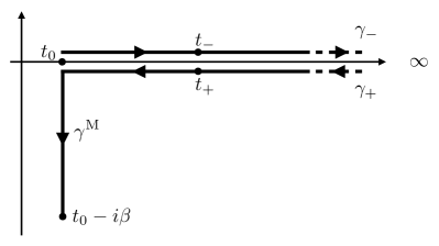
Figure 1: $L$-shaped Konstantinov-Perel’s contour.

Hamiltonian on the contour.– The explicit form of the evolution operators is $\hat{\mbox{$\mathcal{U}$}}(t,t_{0})=T\big{\{}\exp\big{[}-i\int_{t_{0}}^{t}d\bar{t}\,\hat{H}(\bar{t})\big{]}\big{\}}$, with $T$ the time-ordering operator, and $\hat{\mbox{$\mathcal{U}$}}(t_{0},t)=\bar{T}\big{\{}\exp\big{[}i\int_{t_{0}}^{t}d\bar{t}\,\hat{H}(\bar{t})\big{]}\big{\}}$, with $\bar{T}$ the anti-time-ordering operator. Therefore the time-dependent average in Eq. (17) can be written as Wagner (1991); Stefanucci and van Leeuwen (2013)

$$O(t) ={\rm Tr}\big{[}\hat{\rho}\,\bar{T}\big{\{}e^{i\int_{t_{0}}^{t}d\bar{t}\,\hat{H}(\bar{t})}\big{\}}\hat{O}(t)\,T\big{\{}e^{-i\int_{t_{0}}^{t}d\bar{t}\,\hat{H}(\bar{t})}\big{\}}\big{]}$$

$$=\frac{{\rm Tr}\big{[}\mbox{$\mathcal{T}$}\big{\{}e^{-i\int_{\gamma}d\bar{z}\,\hat{H}(\bar{z})}\hat{O}(z)\big{\}}\big{]}}{{\rm Tr}\big{[}\mbox{$\mathcal{T}$}\big{\{}e^{-i\int_{\gamma}d\bar{z}\,\hat{H}(\bar{z})}\big{\}}\big{]}}.$$ (32)

In the second equality $z$ and $\bar{z}$ are contour-times running on the $L$-shaped oriented contour $\gamma$ Konstantinov and Perel (1961) consisting of a forward branch $\gamma_{-}$ going from the initial time $t_{0}$ to $\infty$, a backward branch $\gamma_{+}$ going from $\infty$ to $t_{0}$ and a vertical track on the complex plane $\gamma^{\rm M}$ going from $t_{0}$ to $t_{0}-i\beta$, see Fig. 1, and $\mathcal{T}$ is the contour ordering operator. Henceforth we denote by $z=t_{\pm}$, $\bar{z}=\bar{t}_{\pm}$, $z^{\prime}=t^{\prime}_{\pm}$, etc. contour times on $\gamma_{\pm}$. For any quantity $q(z)$, being it a function or an operator, we define $q(t_{\pm})=q(t)$ and $q(t_{0}-i\tau)=q$ independent of $\tau\in(0,\beta)$. The only exception is $h(\mbox{\boldmath$\nabla$},{\mathbf{r}},t_{0}-i\tau)=h(\mbox{\boldmath$\nabla$},{\mathbf{r}})-\mu$. Thanks to this different definition for $h$ we have $\hat{H}(t_{\pm})=\hat{H}(t)$ and $\hat{H}(t_{0}-i\tau)=\hat{H}-\mu\hat{N}_{e}$. Notice that the Hamiltonian $\hat{H}(z)$ depends on $z$ through the dependence of $h$, $K$, $v$ and $g$, see Eqs. (31).

One remark about the dependence of $\hat{O}(z)$ on $z$. If the operator does not depend on $z$ we can safely write $\hat{O}(t)=\hat{O}$ in the first line of Eq. (32). However, if we do so in the second line then it is not clear where to place the operator $\hat{O}$ after the contour ordering. The reason to keep the contour argument even for operators that do not have an explicit time dependence (like the operators $\hat{\psi}$, $\hat{U}$ and $\hat{P}$) stems from the need of specifying their position along the contour, thus rendering unambiguous the action of $\mathcal{T}$. Once the operators are ordered we can omit the time arguments if there is no time dependence.

To shorten the equations we gather the displacement and momentum operators into a two-dimensional vector of operators having components

$$\hat{\mbox{\boldmath$\phi$}}_{{\mathbf{q}}\nu}=\left(\begin{array}[]{c}\hat{\phi}_{{\mathbf{q}}\nu}^{1}\\ \hat{\phi}_{{\mathbf{q}}\nu}^{2}\end{array}\right)=\left(\begin{array}[]{c}\hat{U}_{{\mathbf{q}}\nu}\\ \hat{P}_{{\mathbf{q}}\nu}\end{array}\right).$$ (37)

The commutation relations for the $\hat{\phi}$-operators follow from the commutation relations $[\hat{U}_{{\mathbf{n}}s,\alpha},\hat{P}_{{\mathbf{n}}^{\prime}s^{\prime},\alpha^{\prime}}]=i\delta_{{\mathbf{n}}{\mathbf{n}}^{\prime}}\delta_{ss^{\prime}}\delta_{\alpha\alpha^{\prime}}$ after inserting the expansions in Eqs. (25) and using the properties in Eq. (26). We find

$$[\hat{\phi}_{{\mathbf{q}}\nu}^{i},\hat{\phi}_{-{\mathbf{q}}^{\prime}\nu^{\prime}}^{i^{\prime}}]=[\hat{\phi}_{{\mathbf{q}}\nu}^{i},\hat{\phi}^{i^{\prime}\,{\dagger}}_{{\mathbf{q}}^{\prime}\nu^{\prime}}]=\delta_{{\mathbf{q}},{\mathbf{q}}^{\prime}}\alpha^{ii^{\prime}}_{\nu\nu^{\prime}}\;,$$ (38)

where

$$\alpha^{ii^{\prime}}_{\nu\nu^{\prime}}=\delta_{\nu\nu^{\prime}}\left(\begin{array}[]{cc}0&i\\ -i&0\end{array}\right)_{ii^{\prime}}.$$ (41)

Let us express the contour Hamiltonian $\hat{H}(z)$, see Eqs. (11) and (31), in terms of the $\hat{\phi}$-operators. We first write the final result and then prove its correctness. We have

$$\hat{H}(z)=\hat{H}_{0,e}^{s}(z)+\hat{H}_{0,ph}^{s}(z)+\hat{H}_{e-e}(z)+\hat{H}_{e-ph}(z),$$ (42)

where

$$\hat{H}_{0,e}^{s}(z)= \!\int\!\!d{\mathbf{x}}\,\hat{\psi}^{{\dagger}}({\mathbf{x}})\Big{[}h(\mbox{\boldmath$\nabla$},{\mathbf{r}},z)-\!\sum_{{\mathbf{q}}\nu}\mbox{\boldmath$g$}_{{\mathbf{q}}\nu}^{{\dagger}}({\mathbf{r}},z)\cdot\mbox{\boldmath$s$}_{{\mathbf{q}}\nu}(z)\Big{]}\hat{\psi}({\mathbf{x}}),$$ (43a)

$$\hat{H}_{0,ph}^{s}(z) =\frac{1}{2}\sum_{{\mathbf{q}}}\sum_{\nu\nu^{\prime}}\hat{\mbox{\boldmath$\phi$}}^{{\dagger}}_{{\mathbf{q}}\nu}\;Q_{\nu\nu^{\prime}}({\mathbf{q}},z)\;\hat{\mbox{\boldmath$\phi$}}_{{\mathbf{q}}\nu^{\prime}}$$

$$\quad+\sum_{{\mathbf{q}}\nu}\int\!d{\mathbf{x}}\,n^{0}({\mathbf{x}})\,\mbox{\boldmath$g$}^{{\dagger}}_{{\mathbf{q}}\nu}({\mathbf{r}},z)\cdot\hat{\mbox{\boldmath$\phi$}}_{{\mathbf{q}}\nu}\;,$$ (43b)

$$\hat{H}_{e-e}(z) =\frac{1}{2}\!\int\!d{\mathbf{x}}d{\mathbf{x}}^{\prime}\hat{\psi}^{{\dagger}}({\mathbf{x}})\hat{\psi}^{{\dagger}}({\mathbf{x}}^{\prime})v({\mathbf{r}},{\mathbf{r}}^{\prime},z)\hat{\psi}({\mathbf{x}}^{\prime})\hat{\psi}({\mathbf{x}}),$$ (43c)

$$\hat{H}_{e-ph}(z) =-\sum_{{\mathbf{q}}\nu}\int\!d{\mathbf{x}}\,\hat{n}({\mathbf{x}})\,\mbox{\boldmath$g$}^{{\dagger}}_{{\mathbf{q}}\nu}({\mathbf{r}},z)\cdot\big{(}\hat{\mbox{\boldmath$\phi$}}_{{\mathbf{q}}\nu}-\mbox{\boldmath$s$}_{{\mathbf{q}}\nu}(z)\big{)},$$ (43d)

and

$$Q_{\nu\nu^{\prime}}({\mathbf{q}},z) =\left(\begin{array}[]{cc}K_{\nu\nu^{\prime}}({\mathbf{q}},z)&0\\ 0&\delta_{\nu\nu^{\prime}},\end{array}\right)$$ (44c)

$$\mbox{\boldmath$g$}_{{\mathbf{q}}\nu}({\mathbf{r}},z) =\left(\begin{array}[]{c}g_{{\mathbf{q}}\nu}({\mathbf{r}},z)\\ 0\end{array}\right).$$ (44f)

In Eqs. (43a) and (43d) we introduce a (two-dimensional vector) shift $\mbox{\boldmath$s$}_{{\mathbf{q}}\nu}(z)$ with the purpose of simplifying the NEGF treatment, see below. The exact form of the shift is irrelevant for the time being as the terms containing $\mbox{\boldmath$s$}_{{\mathbf{q}}\nu}(z)$ cancel out in the sum of Eq. (42), thereby $\hat{H}(z)$ is independent of this quantity. The shifted electronic Hamiltonian $\hat{H}_{0,e}^{s}(z)$ evaluated at zero shift, i.e., $\mbox{\boldmath$s$}_{{\mathbf{q}}\nu}(z)=0$, is the same as $\hat{H}_{0,e}(z)$, see Eqs. (12) and (31a). The first term of the shifted phononic Hamiltonian $\hat{H}_{0,ph}^{s}(z)$ is the same as $\hat{H}_{0,ph}(z)$, see Eqs. (27) and (31b), whereas the second term coincides with the contribution to $\hat{H}^{\prime}$ coming from $n^{0}$ in $\Delta\hat{n}$, see Eqs. (28) and (31d). The $e$-$e$ interaction Hamiltonian $\hat{H}_{e-e}(z)$ has not changed, see Eqs. (11) and (31c). Finally, the $e$-$ph$ interaction Hamiltonian $\hat{H}_{e-ph}(z)$ evaluated at zero shift coincides with the contribution to $\hat{H}^{\prime}$ coming from $\hat{n}$ in $\Delta\hat{n}$. We conclude that Eq. (42) is identical to the contour Hamiltonian for any two-dimensional vector $\mbox{\boldmath$s$}_{{\mathbf{q}}\nu}(z)$.

IV Equations of motion for operators in the contour Heisenberg picture

The contour Heisenberg picture is an extremely useful concept to develop the NEGF formalism. We define the contour evolution operators according to

$$\hat{\mbox{$\mathcal{U}$}}(z,t_{0}) =\mbox{$\mathcal{T}$}\big{\{}e^{-i\int_{t_{0}}^{z}d\bar{z}\,\hat{H}(\bar{z})}\big{\}}$$ (45a)

$$\hat{\mbox{$\mathcal{U}$}}(t_{0},z) =\bar{\mbox{$\mathcal{T}$}}\big{\{}e^{i\int_{t_{0}}^{z}d\bar{z}\,\hat{H}(\bar{z})}\big{\}}$$ (45b)

where $\bar{\mbox{$\mathcal{T}$}}$ is the anti-contour-ordering operator. These operators are unitary for $z=t_{\pm}$ and hermitian for $z=t_{0}-i\beta$. For all $z\in\gamma$ we have the property $\hat{\mbox{$\mathcal{U}$}}(t_{0},z)\hat{\mbox{$\mathcal{U}$}}(z,t_{0})=1$. We define an operator in the contour Heisenberg picture as

$$\hat{O}_{H}(z)\equiv\hat{\mbox{$\mathcal{U}$}}(t_{0},z)\hat{O}(z)\hat{\mbox{$\mathcal{U}$}}(z,t_{0}).$$ (46)

It is straightforward to verify that $O_{H}(t_{\pm})=O_{H}(t)$. The equation of motion for operators in the contour Heisenberg picture follows directly from the definitions in Eqs. (45)

$$i\frac{d\hat{O}_{H}(z)}{dz}=\hat{\mbox{$\mathcal{U}$}}(t_{0},z)\Big{(}[\hat{O}(z),\hat{H}(z)]+i\frac{dO(z)}{dz}\Big{)}\hat{\mbox{$\mathcal{U}$}}(z,t_{0}).$$ (47)

As the Hamiltonian is written in terms of $\hat{\psi}({\mathbf{x}})$ and $\hat{\mbox{\boldmath$\phi$}}_{{\mathbf{q}}\nu}$ it is clear that the equation of motion for these operators plays a crucial role in the following derivation.

Equations of motion.– Using Eq. (47) the equation of motion for the $\hat{\phi}$-operators reads

$$\sum_{\nu^{\prime}}\Big{[}i\frac{d}{dz}\alpha_{\nu\nu^{\prime}} -Q_{\nu\nu^{\prime}}({\mathbf{q}},z)\Big{]}\hat{\mbox{\boldmath$\phi$}}_{{\mathbf{q}}\nu^{\prime},H}(z)$$

$$=-\int\!d{\mathbf{x}}\,\mbox{\boldmath$g$}_{{\mathbf{q}}\nu}({\mathbf{r}},z)\big{(}\hat{n}_{H}({\mathbf{x}},z)-n^{0}({\mathbf{x}})\big{)}.$$ (48)

To remove the inhomogeneous term with $n^{0}$ we define the $2\times 2$ GF $D_{0,{\mathbf{q}}\nu\nu^{\prime}}$ as the solution of

$$\sum_{\bar{\nu}}\Big{[}i\frac{d}{dz}\alpha_{\nu\bar{\nu}} -Q_{\nu\bar{\nu}}({\mathbf{q}},z)\Big{]}D_{0,{\mathbf{q}}\bar{\nu}\nu^{\prime}}(z,z^{\prime})=\mathbb{1}\delta_{\nu\nu^{\prime}}\delta(z,z^{\prime}),$$ (49)

and satisfying the periodic Kubo-Martin-Schwinger (KMS) boundary conditions along the contour $\gamma$. We use $D_{0}$ to define the shift in Eqs. (43)

$$\mbox{\boldmath$s$}_{{\mathbf{q}}\nu^{\prime}}(z)=\sum_{\bar{\nu}}\int\!d\bar{z}\,D_{0,{\mathbf{q}}\nu^{\prime}\bar{\nu}}(z,\bar{z})\int\!d{\mathbf{x}}\,\mbox{\boldmath$g$}_{{\mathbf{q}}\bar{\nu}}({\mathbf{r}},\bar{z})n^{0}({\mathbf{x}}).$$ (50)

Then the equation of motion for the (time-dependent) shifted displacement

$$\hat{\mbox{\boldmath$\varphi$}}_{{\mathbf{q}}\nu}(z)\equiv\hat{\mbox{\boldmath$\phi$}}_{{\mathbf{q}}\nu}-\mbox{\boldmath$s$}_{{\mathbf{q}}\nu}(z)$$ (51)

reads

$$\sum_{\nu^{\prime}}\Big{[}i\frac{d}{dz}\alpha_{\nu\nu^{\prime}}-Q_{\nu\nu^{\prime}} ({\mathbf{q}},z)\Big{]}\hat{\mbox{\boldmath$\varphi$}}_{{\mathbf{q}}\nu^{\prime},H}(z)$$

$$=-\int\!d{\mathbf{x}}\,\mbox{\boldmath$g$}_{{\mathbf{q}}\nu}({\mathbf{r}},z)\,\hat{n}_{H}({\mathbf{x}},z),$$ (52)

which is a homogeneous equation in the field operators. Notice that the shift is proportional to the identity operator and therefore $\mbox{\boldmath$s$}_{{\mathbf{q}}\nu,H}(z)=\mbox{\boldmath$s$}_{{\mathbf{q}}\nu}(z)$. Such proportionality also implies that the operators $\hat{\mbox{\boldmath$\varphi$}}(z)$ and $\hat{\mbox{\boldmath$\phi$}}(z^{\prime})$ [these operators are not in the contour-Heisenberg picture and in particular $\hat{\mbox{\boldmath$\phi$}}(z^{\prime})$ does not depend on $z^{\prime}$] satisfy the same commutation relations for any $z$ and $z^{\prime}$ :

$$[\hat{\varphi}_{{\mathbf{q}}\nu}^{i}(z),\hat{\varphi}^{i^{\prime}\,{\dagger}}_{{\mathbf{q}}^{\prime}\nu^{\prime}}(z^{\prime})]=[\hat{\varphi}_{{\mathbf{q}}\nu}^{i}(z),\hat{\phi}^{i^{\prime}\,{\dagger}}_{{\mathbf{q}}^{\prime}\nu^{\prime}}(z^{\prime})]=[\hat{\phi}_{{\mathbf{q}}\nu}^{i}(z),\hat{\phi}^{i^{\prime}\,{\dagger}}_{{\mathbf{q}}^{\prime}\nu^{\prime}}(z^{\prime})].$$ (53)

From the commutator $[\hat{\psi}({\mathbf{x}}),\hat{H}(z)]$ we can easily derive the equation of motion for the electronic field operators

$$\Big{[}i\frac{d}{dz}-h^{s}(\mbox{\boldmath$\nabla$},{\mathbf{r}},z)\Big{]} \hat{\psi}_{H}({\mathbf{x}},z)$$

$$=\int d{\mathbf{x}}^{\prime}v({\mathbf{r}},{\mathbf{r}}^{\prime},z)\hat{n}_{H}({\mathbf{x}}^{\prime},z)\hat{\psi}_{H}({\mathbf{x}},z)$$

$$-\sum_{{\mathbf{q}}\nu}\hat{\psi}_{H}({\mathbf{x}},z)\,\mbox{\boldmath$g$}_{{\mathbf{q}}\nu}^{{\dagger}}({\mathbf{r}},z)\cdot\hat{\mbox{\boldmath$\varphi$}}_{{\mathbf{q}}\nu,H}(z),$$ (54)

where we define the shifted one-particle Hamiltonian

$$h^{s}(\mbox{\boldmath$\nabla$},{\mathbf{r}},z)\equiv h(\mbox{\boldmath$\nabla$},{\mathbf{r}},z)-\!\sum_{{\mathbf{q}}\nu}\mbox{\boldmath$g$}_{{\mathbf{q}}\nu}^{{\dagger}}({\mathbf{r}},z)\cdot\mbox{\boldmath$s$}_{{\mathbf{q}}\nu}(z),$$ (55)

see Eq. (43a), and in the last term of the r.h.s. we recognize that the density operator in Eq. (43d) multiples the shifted displacement $\hat{\mbox{\boldmath$\varphi$}}$ defined in Eq. (51).

V Green’s functions and Martin-Schwinger hierarchy

The building blocks of the NEGF formalism are the electronic and phononic GF. Let us introduce a notation which is used throughout the reminder of the paper. We denote the position, spin and contour-time coordinates of an electronic field operator with the collective indices

$$k ={\mathbf{x}}_{k},z_{k},\;\;\;\;j={\mathbf{x}}_{j},z_{j},\;\;\;\ldots$$

$$k^{\prime} ={\mathbf{x}}_{k}^{\prime},z_{k}^{\prime},\;\;\;\;j^{\prime}={\mathbf{x}}_{j}^{\prime},z_{j}^{\prime},\;\;\;\ldots$$ (56)

etc.. Thus, for instance, $\hat{\psi}(1)=\hat{\psi}({\mathbf{x}}_{1},z_{1})$ and $\hat{\psi}(2^{\prime})=\hat{\psi}({\mathbf{x}}_{2}^{\prime},z_{2}^{\prime})$. We recall that the electronic field operators have no explicit dependence on the contour-time, i.e., $\hat{\psi}({\mathbf{x}},z)=\hat{\psi}({\mathbf{x}})$. Without any risk of ambiguity we use the same notation to denote the momentum, branch, component and contour-time coordinates of a phononic field operator

$$k ={\mathbf{q}}_{k},\nu_{k},i_{k},z_{k},\;\;\;\;j={\mathbf{q}}_{j},\nu_{j},i_{j},z_{j},\;\;\;\ldots$$

$$k^{\prime} ={\mathbf{q}}^{\prime}_{k},\nu^{\prime}_{k},i^{\prime}_{k},z^{\prime}_{k},\;\;\;\;j^{\prime}={\mathbf{q}}^{\prime}_{j},\nu^{\prime}_{j},i^{\prime}_{j},z^{\prime}_{j},\;\;\;\ldots$$ (57)

etc.. Thus, for instance, $\hat{\varphi}(1)=\hat{\varphi}_{{\mathbf{q}}_{1}\nu_{1}}^{i_{1}}(z_{1})$ and $\hat{\varphi}(2^{\prime})=\hat{\varphi}_{{\mathbf{q}}^{\prime}_{2}\nu^{\prime}_{2}}^{i^{\prime}_{2}}(z^{\prime}_{2})$. We also use the superscript star “ ^∗ ” to denote the composite index with reversed momentum, e.g., $k^{\ast}=-{\mathbf{q}}_{k},\nu_{k},i_{k},z_{k}$. Of course starring twice is the same as no starring, i.e., $k^{\ast\ast}=k$. We then define

$$\overrightarrow{D}_{0}^{-1}(1,2) \equiv\Big{[}i\frac{d}{dz_{1}}\alpha^{i_{1}i_{2}}_{\nu_{1}\nu_{2}}-Q^{i_{1}i_{2}}_{\nu_{1}\nu_{2}}({\mathbf{q}}_{1},z_{1})\big{]}\delta_{{\mathbf{q}}_{1}{\mathbf{q}}_{2}}\delta(z_{1},z_{2})$$ (58a)

$$\overrightarrow{G}_{0}^{-1}(1;2) \equiv\Big{[}i\frac{d}{dz_{1}}-h^{s}(\mbox{\boldmath$\nabla$}_{1},{\mathbf{r}}_{1},z_{1})\Big{]}\delta({\mathbf{x}}_{1}-{\mathbf{x}}_{2})\delta(z_{1},z_{2}),$$ (58b)

$$g(1;2) \equiv\delta(z_{1},z_{2})g^{i_{2}}_{{\mathbf{q}}_{2}\nu_{2}}({\mathbf{r}}_{1},z_{1}),$$ (58c)

$$v(1;2) \equiv\delta(z_{1},z_{2})v({\mathbf{r}}_{1},{\mathbf{r}}_{2},z_{1}),$$ (58d)

where $\delta(z_{1},z_{2})$ is the Dirac-delta on the contour Stefanucci and van Leeuwen (2013). Accordingly, the equations of motion for the field operators, i.e., Eqs. (52) and (54), are shortened as

$$\int\!d\tilde{2}\,\overrightarrow{D}_{0}^{-1}(1,\tilde{2})\hat{\varphi}_{H}(\tilde{2}) =-\int\!d\bar{2}\,g(\bar{2};1)\hat{\psi}^{{\dagger}}_{H}(\bar{2})\hat{\psi}_{H}(\bar{2}),$$ (59a)

$$\int\!d\bar{2}\,\overrightarrow{G}_{0}^{-1}(1;\bar{2})\,\hat{\psi}_{H}(\bar{2}) =\int\!d\bar{2}\,v(1;\bar{2})\hat{\psi}^{{\dagger}}_{H}(\bar{2})\hat{\psi}_{H}(\bar{2})\hat{\psi}_{H}(1)$$

$$-\int\!d\tilde{2}\,g(1;\tilde{2}^{\ast})\hat{\psi}_{H}(1)\hat{\varphi}_{H}(\tilde{2}).$$ (59b)

To distinguish the integration variables of the electronic operators $\hat{\psi}$ from those of the phononic operators $\hat{\varphi}$ we use a bar for the former and a tilde for the latter, thus $\int d\bar{1}\equiv\int d\bar{{\mathbf{x}}}_{1}d\bar{z}_{1}$ and $\int d\tilde{1}\equiv\sum_{\tilde{q}_{1}\tilde{\nu}_{1}\tilde{i}_{1}}\int d\tilde{z}_{1}$. Setting $v=g=0$ in the r.h.s. of Eqs. (59) we obtain the equations of motion of the field operators governed by the Hamiltonian

$$\hat{H}_{0}^{s}(z)\equiv\hat{H}_{0,e}^{s}(z)+\hat{H}_{0,ph}^{s}(z).$$ (60)

We shall use this observation in the next section.

Green’s functions.– The phononic and electronic GF are contour-ordered correlators of strings of phononic and electronic field operators. The $m$-particle phononic GF is defined as

$$\widetilde{D}_{m} (1,2,...,2m)\equiv\frac{1}{i^{m}}{\rm Tr}\left[\hat{\rho}\,\mbox{$\mathcal{T}$}\left\{\hat{\varphi}_{H}(1)\hat{\varphi}_{H}(2)...\hat{\varphi}_{H}(2m)\right\}\right]=\frac{1}{i^{m}}\frac{{\rm Tr}\left[\mbox{$\mathcal{T}$}\left\{e^{-i\int_{\gamma}d\bar{z}\hat{H}(\bar{z})}\hat{\varphi}(1)\hat{\varphi}(2)...\hat{\varphi}(2m)\right\}\right]}{{\rm Tr}\left[\mbox{$\mathcal{T}$}\left\{e^{-i\int_{\gamma}d\bar{z}\hat{H}(\bar{z})}\right\}\right]}.$$ (61)

In this definition $m$ can also be a half-integer; in particular $\widetilde{D}_{1/2}(1)=\varphi(1)/i^{1/2}$. The phononic GF $\widetilde{D}_{m}$ differs from that in Refs. Säkkinen et al. (2015a); Karlsson and van Leeuwen (2020) as it is defined in terms of the shifted operators $\hat{\varphi}$ instead of $\hat{\phi}$. We observe that the operators appearing in the second equality are not in the contour Heisenberg picture [compare with Eq. (32)]. The phononic GF is totally symmetric under an arbitrary permutation of its arguments $1,2,...,2m$. Similarly, we define the $n$-particle electronic GF as

$$G_{n} (1,...,n;1^{\prime},...,n^{\prime})=\frac{1}{i^{n}}{\rm Tr}\left[\hat{\rho}\,\mbox{$\mathcal{T}$}\big{\{}\hat{\psi}_{H}(1)...\hat{\psi}_{H}(n)\hat{\psi}^{{\dagger}}_{H}(n^{\prime})...\hat{\psi}^{{\dagger}}_{H}(1^{\prime})\big{\}}\right]=\frac{1}{i^{n}}\frac{{\rm Tr}\left[\mbox{$\mathcal{T}$}\left\{e^{-i\int_{\gamma}d\bar{z}\hat{H}(\bar{z})}\hat{\psi}(1)...\hat{\psi}(n)\hat{\psi}^{{\dagger}}(n^{\prime})...\hat{\psi}^{{\dagger}}(1^{\prime})\right\}\right]}{{\rm Tr}\left[\mbox{$\mathcal{T}$}\left\{e^{-i\int_{\gamma}d\bar{z}\hat{H}(\bar{z})}\right\}\right]}.$$

The electronic GF is totally antisymmetric under an arbitrary permutation of the arguments $1,2,...,n$ and $1^{\prime},2^{\prime},...,n^{\prime}$.

Martin-Schwinger hierarchy.– Taking into account that the commutation relations for the operators $\hat{\varphi}$ are identical to the commutation relations for the operators $\hat{\phi}$, see Eq. (53), the equations of motion for $\widetilde{D}_{m}$ with $m=1/2,1,3/2,...$ read

$$\int d\tilde{1}\,\overrightarrow{D}_{0}^{-1}(k,\tilde{1})\widetilde{D}_{m}(1,...,\tilde{1},...,2m) =-\frac{1}{i^{m}}\int d\bar{1}\,g(\bar{1};k)\,{\rm Tr}\Big{[}\hat{\rho}\;\mbox{$\mathcal{T}$}\Big{\{}\hat{\varphi}_{H}(1),...,\underbrace{\hat{\psi}^{{\dagger}}_{H}(\bar{1})\hat{\psi}_{H}(\bar{1})}_{k-{\rm th\,place}},...,\hat{\varphi}_{H}(2m)\Big{\}}\Big{]}$$

$$+\sum_{\begin{subarray}{c}j=1\\ j\neq k\end{subarray}}^{2m}\delta(k,j^{\ast})\widetilde{D}_{m-1}(1,...,\stackrel{{\scriptstyle\sqcap}}{{k}},...,\stackrel{{\scriptstyle\sqcap}}{{j}},...,2m),$$ (63)

where the variable $\tilde{1}$ in the l.h.s. is at place $k$ and we define $\widetilde{D}_{0}=1$ and $\widetilde{D}_{-1/2}=0$. The first term in the r.h.s. originates from the equation of motion Eq. (59a). The last term in the r.h.s. originates from the derivative of the Heaviside step-functions implicit in the contour ordering Stefanucci and van Leeuwen (2013). These derivatives generate quantities like $\delta(z_{k},z_{j})[\hat{\varphi}^{i_{k}}_{{\mathbf{q}}_{k}\nu_{k},H}(z_{k}),\hat{\varphi}^{i_{j}}_{{\mathbf{q}}_{j}\nu_{j},H}(z_{j})]=\delta(z_{k},z_{j})\delta_{{\mathbf{q}}_{k},-{\mathbf{q}}_{j}}\alpha^{i_{k}i_{j}}_{\nu_{k}\nu_{j}}$, see Eq. (38), which multiplied by $\alpha$ lead to $\delta(k,j^{\ast})\equiv\delta(z_{k},z_{j})\delta_{{\mathbf{q}}_{k},-{\mathbf{q}}_{j}}\delta_{\nu_{k}\nu_{j}}\delta_{i_{k}i_{j}}$. To shorten the equations we have also introduced the symbol “ $\sqcap$ ” above an index to indicate that the index is missing from the list. In a similar way we can derive the equations of motion for the $n$-particle GF and find for $n=1,2,3,\ldots$

$$\int d\bar{1}\,\overrightarrow{G}_{0}^{-1}(k;\bar{1})G_{n}(1,...,\bar{1},...,n;1^{\prime},...,n^{\prime}) =-\,i\int d\bar{1}\,v(k;\bar{1})\,G_{n+1}(1,...,n,\bar{1};1^{\prime},...,n^{\prime},\bar{1}^{+})$$

$$-\frac{1}{i^{n}}\int d\tilde{1}\,g(k;\tilde{1}^{\ast}){\rm Tr}\Big{[}\hat{\rho}\;\mbox{$\mathcal{T}$}\Big{\{}\hat{\psi}_{H}(1),...,\underbrace{\hat{\psi}_{H}(k)\hat{\varphi}_{H}(\tilde{1})}_{k-{\rm th\,place}},...,\hat{\psi}_{H}(n)\hat{\psi}_{H}(n^{\prime}),...,\hat{\psi}^{{\dagger}}_{H}(1^{\prime})\Big{\}}\Big{]}$$

$$+\sum_{j=1}^{n}\,(-)^{k+j}\,\delta(k;j^{\prime})\,G_{n-1}(1,...,\stackrel{{\scriptstyle\sqcap}}{{k}},...,n;1^{\prime},...,\stackrel{{\scriptstyle\sqcap}}{{j^{\prime}}},...,n^{\prime}),$$ (64)

where the variable $\bar{1}$ in the l.h.s. is at place $k$ and we define $G_{0}=1$. The first two terms in the r.h.s. originate from the equation of motion Eq. (59b). The last term in the r.h.s. originates from the the derivative of the Heaviside step-functions implicit in the contour ordering. In the electronic case $\delta(k;j)\equiv\delta({\mathbf{x}}_{k}-{\mathbf{x}}_{j})\delta(z_{k},z_{j})$. We further notice that the last argument of the GF $G_{n+1}$ is $\bar{1}^{+}$. We use the superscript “ $+$ ” to indicate that the contour time is infinitesimally later than $\bar{z}_{1}$. This infinitesimal shift guarantees that the creation operator $\hat{\psi}^{{\dagger}}(\bar{1})$ in $G_{n+1}$ ends up to the left of the annihilation operator $\hat{\psi}(\bar{1})$ when the operators are contour ordered.

The equation of motion for $G_{n}$ with derivative with respect to the primed arguments can be worked out similarly. All equations of motion must be solved with KMS boundary conditions, i.e., $\widetilde{D}_{m}$ must be periodic on the contour with respect to all times $z_{1},\ldots,z_{2m}$ and $G_{n}$ must be antiperiodic on the contour with respect to all times $z_{1},\ldots,z_{n},z^{\prime}_{1},\ldots,z^{\prime}_{n}$.

If the $e$-$ph$ coupling $g=0$ then $\widetilde{D}_{m}$ couples only to $\widetilde{D}_{m-1}$. In the electronic sector things are different. For $g=0$ the equations of motion reduce to the Martin-Schwinger hierarchy for a system of only electrons, and $G_{n}$ couples to $G_{n-1}$ and $G_{n+1}$ through the Coulomb interaction $v$. For $G_{n}$ to couple only to $G_{n-1}$ the Coulomb interaction has to vanish too.

When both $e$-$e$ and $e$-$ph$ interactions are present, $G_{n}$ couples to $G_{n-1}$, $G_{n+1}$ as well as to mixed GF consisting of a mix string of $\hat{\psi}$, $\hat{\psi}^{{\dagger}}$, and $\hat{\varphi}$ operators, see second line in the equations of motion. Likewise, $\widetilde{D}_{m}$ couples to $\widetilde{D}_{m-1}$ but also to mixed GF, see first term in the r.h.s. of the equations of motion. The equations of motion for the mixed GF can be derived in precisely the same way, see also Ref. sak . We refer to the full set of equations as the Martin-Schwinger hierarchy for electron-phonon systems. In the next sections we lay down a perturbative method to calculate all GF.

VI Wick’s theorem for the many-particle Green’s functions

The Wick theorem provides the solution of the Martin-Schwinger hierarchy with r.h.s evaluated at $g=v=0$. This is the same as solving the Martin-Schwinger hierarchy for a system of electrons and phonons governed by the Hamiltonian $\hat{H}_{0}^{s}$, see comment above Eq. (60). As $\hat{H}_{0}^{s}$ depends on $g$ explicitly, setting $g=v=0$ in the r.h.s. of Eqs. (63) and (64) is not the same as solving the Martin-Schwinger hierarchy with $\hat{H}|_{g=v=0}$ (noninteracting hierarchy). Henceforth we name the GF governed by $\hat{H}_{0}^{s}$ as the independent GF and we denote them by $D_{0,m}$ and $G_{0,n}$. We then have

$$\int\!d\tilde{1}\,\overrightarrow{D}_{0}^{-1}(k,\tilde{1})D_{0,m}(1,...,\tilde{1},...,2m) =\sum_{\begin{subarray}{c}j=1\\ j\neq k\end{subarray}}^{2m}\delta(k,j^{\ast})D_{0,m-1}(1,...,\stackrel{{\scriptstyle\sqcap}}{{k}},...,\stackrel{{\scriptstyle\sqcap}}{{j}},...,2m),$$ (65a)

$$\int d\bar{1}\,\overrightarrow{G}_{0}^{-1}(k;\bar{1})G_{0,n}(1,...,\bar{1},...,n;1^{\prime},...,n^{\prime}) =\sum_{j=1}^{n}\,(-)^{k+j}\,\delta(k;j^{\prime})\,G_{0,n-1}(1,...,\stackrel{{\scriptstyle\sqcap}}{{k}},...,n;1^{\prime},...,\stackrel{{\scriptstyle\sqcap}}{{j^{\prime}}},...,n^{\prime}),$$ (65b)

and the like with time derivatives with respect to the primed arguments. The independent GF satisfy two independent hierarchies. Despite the similarities the phononic and electronic hierarchies present important differences. The sum in the r.h.s. runs over all arguments of $D_{0,m}$ in Eq. (65a) whereas it runs only over the unprimed arguments of $G_{0,n}$ in Eq. (64). Moreover, in the phononic case $m$ can also be a half-integer. From Eq. (65a) we see that the integer $m$ connects with the integer $m-1$ and the half-integer $m$ connects with the half-integer $m-1$. Therefore, we have two separate hierarchies of equations for the phononic GF.

Wick’s theorem for phonons.– The proof of Wick’s theorem for $D_{0,m}$ goes along the same lines as in Ref. Karlsson and van Leeuwen (2020). The phononic GF $D_{0,m}=0$ for all half-integers $m$. This can easily be proven by considering the average of the equation of motion Eq. (52) with $g=0$. By definition this average is proportional to $D_{0,1/2}$ and the only solution satisfying the KMS boundary conditions is $D_{0,1/2}=0$. Consider now $m=3/2$:

$$\int d\tilde{1}\, \overrightarrow{D}_{0}^{-1}(1,\tilde{1})D_{0,3/2}(\tilde{1},2,3)$$

$$=\delta(1,2^{\ast})D_{0,1/2}(3)+\delta(1,3^{\ast})D_{0,1/2}(2)=0,$$ (66)

and the like for the variables $2$ and $3$. We see that $D_{0,3/2}=0$ is a solution satisfying the KMS boundary conditions. By induction, $D_{0,m}=0$ for half-integers. Henceforth we only consider integers $m$ in the noninteracting case.

For $m=1$ we have the equation of motion for $D_{0,1}$:

$$\int d\tilde{1}\,\overrightarrow{D}_{0}^{-1}(1,\tilde{1})D_{0,1}(\tilde{1},2)=\delta(1,2^{\ast}),$$ (67)

Comparing with Eq. (49) we realize that

$$D_{0,1}(1,2)=\delta_{{\mathbf{q}}_{1},-{\mathbf{q}}_{2}}D_{0,{\mathbf{q}}_{1}\nu_{1}\nu_{2}}^{i_{1}i_{2}}(z_{1},z_{2}).$$ (68)

Without any risk of ambiguity we denote $D_{0,1}(1,2)$ simply by $D_{0}(1,2)$ in the remainder of the paper. For $D_{0,m}$ with $m>1$ the solution of Eq. (65a) is given by the so-called hafnian Caianiello (1973); Itzykson and Zuber (1980); sak . The hafnian can be defined recursively starting from any of the arguments in $D_{0,m}$. Choosing for instance the argument $k$ we have

$$D_{0,m}(1,...,2m)=\sum_{\begin{subarray}{c}j=1\\ j\neq k\end{subarray}}^{2m}D_{0}(k,j)D_{0,m-1}(1,...,\stackrel{{\scriptstyle\sqcap}}{{k}},...,\stackrel{{\scriptstyle\sqcap}}{{j}},...,2m).$$ (69)

Using again Eq. (69) for $D_{0,m-1}$ and then for $D_{0,m-2}$ and so on and so forth we obtain an expansion of $D_{0,m}$ in terms of products of $m$ $D_{0}$’s. A compact way to write this expansion is

$$D_{0,m}(1,...,2m)=\frac{1}{2^{m}m!}\sum_{P} D_{0}(P(1),P(2))\ldots$$

$$\times D_{0}(P(2m-1),P(2m)),$$ (70)

where the sum runs over all permutations of the indices $1,2,\ldots,2m$. The recursive form of Eq. (69) makes it clear that $D_{0,m}$ satisfies Eq. (65a) and the KMS boundary conditions.

Wick’s theorem for electrons.– The solution of Eq. (64) has been discussed at length in Refs. van Leeuwen and Stefanucci (2012); Stefanucci and van Leeuwen (2013). We here write the final result for completeness. For $n=1$ Eq. (64) yields

$$\int d\bar{1}\,\overrightarrow{G}_{0}^{-1}(1;\bar{1})G_{0,1}(\bar{1};2)=\delta(1;2),$$ (71)

to be solved with KMS boundary conditions. Like for the phononic case we shorten the notation and write $G_{0,1}(1;2)=G_{0}^{s}(1;2)$. The superscript “ $s$ ” reminds us that this GF depends on $g$ through $h^{s}$. For $G_{0,n}$ with $n>1$ the solution of Eq. (64) is again defined recursively choosing either an unprimed or a primed argument

$$G_{0,n}(1,...,n;1^{\prime},...,n^{\prime}) =\sum_{k=1}^{n}\,(-)^{k+j}G_{0}^{s}(k;j^{\prime})$$

$$\times G_{0,n-1}(1,...,\stackrel{{\scriptstyle\sqcap}}{{k}},...,n;1^{\prime},...,\stackrel{{\scriptstyle\sqcap}}{{j^{\prime}}},...,n^{\prime})$$

$$=\sum_{j=1}^{n}(-)^{k+j}G_{0}^{s}(k;j^{\prime})$$

$$\times G_{0,n-1}(1,...,\stackrel{{\scriptstyle\sqcap}}{{k}},...,n;1^{\prime},...,\stackrel{{\scriptstyle\sqcap}}{{j^{\prime}}},...,n^{\prime}).$$ (72)

Using again Eq. (72) for $G_{0,n-1}$ and then for $G_{0,n-2}$ and so on and so forth we obtain an expansion of $G_{0,n}$ in terms of products of $n$ $G^{s}_{0}$’s. A compact way to write this expansion is the determinant

$$G_{0,n}(1,...,n;1^{\prime},...,n^{\prime}) =\left|\begin{array}[]{ccc}G_{0}^{s}(1;1^{\prime})&\ldots&G_{0}^{s}(1;n^{\prime})\\ \vdots&&\vdots\\ G_{0}^{s}(n;1^{\prime})&\ldots&G_{0}^{s}(n;n^{\prime})\end{array}\right|$$ (76)

$$=\sum_{P}(-)^{P} G_{0}^{s}(P(1);1^{\prime})\ldots G_{0}^{s}(P(n);n^{\prime})$$ (77)

where the sum runs over all permutations of the indices $1,2,...,n$ and $(-)^{P}$ is the sign of the permutation.

The recursive form of the Wick’s theorem highlights the differences between the phononic and the electronic case. For $G_{0,n}$ we need to connect unprimed arguments to primed arguments in all possible ways. For $D_{0,m}$ there is no such distinction, and we need to connect all arguments in all possible ways.

VII Exact Green’s functions from Wick’s theorem

The interacting GF $\widetilde{D}_{m}$ and $G_{n}$ can be expanded in powers of the $e$-$e$ interaction $v$ and $e$-$ph$ coupling $g$. In this section we focus on the one-particle electronic GF $G\equiv G_{1}$, the one-particle phononic GF $\widetilde{D}\equiv\widetilde{D}_{1}$ and the half-particle phononic GF $\widetilde{D}_{1/2}$. The final results are Eqs. (85), (87) and (88). In Section IX we show that the perturbative expansion leads to a closed system of equations for these quantities. Higher order Green’s functions as well as mixed Green’s functions (relevant for linear response theory) can be investigated along the same lines, see Ref. Stefanucci and van Leeuwen (2013).

The starting point is the Hamiltonian written in the form of Eq. (42), i.e., $\hat{H}=\hat{H}_{0}^{s}+\hat{H}_{e-e}+\hat{H}_{e-ph}$ with $\hat{H}_{0}^{s}$ defined in Eq. (60). Inside the contour-ordering the Hamiltonians $\hat{H}_{0}^{s}$, $\hat{H}_{e-e}$ and $\hat{H}_{e-ph}$ can be treated as commuting operators and hence the exponential of their sum can be separated into the product of three exponentials. It is then natural to define the independent averages as

$$\langle\mbox{$\mathcal{T}$}\big{\{}\ldots\big{\}}\rangle^{s}_{\rm 0}\equiv{\rm Tr}\Big{[}\mbox{$\mathcal{T}$}\big{\{}e^{-i\int_{\gamma}d\bar{z}\hat{H}^{s}_{0}(\bar{z})}\ldots\big{\}}\Big{]}.$$ (78)

We emphasize again that the independent averages are not the same as the noninteracting averages, i.e., the averages with $v=g=0$, since both $\hat{H}_{0,e}^{s}$ and $\hat{H}_{0,ph}^{s}$ depend on $g$, see Eqs.(43a) and (43b).

One-particle electronic Green’s function.– The GF $G\equiv G_{1}$ is defined in Eq. (LABEL:manyGF1). We have

$$G(a;b) =\frac{1}{i}\frac{{\rm Tr}\left[\mbox{$\mathcal{T}$}\left\{e^{-i\int_{\gamma}d\bar{z}\,\hat{H}_{0}^{s}(\bar{z})}e^{-i\int_{\gamma}d\bar{z}\,\hat{H}_{e-e}(\bar{z})}e^{-i\int_{\gamma}d\bar{z}\,\hat{H}_{e-ph}(\bar{z})}\hat{\psi}(a)\hat{\psi}^{{\dagger}}(b)\right\}\right]}{{\rm Tr}\left[\mbox{$\mathcal{T}$}\left\{e^{-i\int_{\gamma}d\bar{z}\,\hat{H}_{0}^{s}(\bar{z})}e^{-i\int_{\gamma}d\bar{z}\,\hat{H}_{e-e}(\bar{z})}e^{-i\int_{\gamma}d\bar{z}\,\hat{H}_{e-ph}(\bar{z})}\right\}\right]},$$ (79)

where $a={\mathbf{x}}_{a},z_{a}$ and $b={\mathbf{x}}_{b},z_{b}$ in accordance with the notation of Eq. (56). The denominator in this equation is the interacting partition function $\mbox{$\mathcal{Z}$}={\rm Tr}[e^{-\beta(\hat{H}-\mu\hat{N}_{e})}]$. Expanding the exponentials containing $\hat{H}_{e-e}$ and $\hat{H}_{e-ph}$ we find

$$G(a;b) =\frac{1}{i}\frac{\sum_{k,p=0}^{\infty}\frac{(-i)^{k+p}}{k!\,p!}\int_{\gamma}\!dz_{1}...dz_{k}d\tilde{z}_{1}...d\tilde{z}_{p}\langle\mbox{$\mathcal{T}$}\Big{\{}\!\hat{H}_{e-e}(z_{1})...\hat{H}_{e-e}(z_{k})\hat{H}_{e-ph}(\tilde{z}_{1})...\hat{H}_{e-ph}(\tilde{z}_{p})\hat{\psi}(a)\hat{\psi}^{{\dagger}}(b)\!\Big{\}}\rangle_{0}^{s}}{\sum_{k,p=0}^{\infty}\frac{(-i)^{k+p}}{k!\,p!}\int_{\gamma}\!dz_{1}...dz_{k}d\tilde{z}_{1}...d\tilde{z}_{p}\langle\mbox{$\mathcal{T}$}\Big{\{}\!\hat{H}_{e-e}(z_{1})...\hat{H}_{e-e}(z_{k})\hat{H}_{e-ph}(\tilde{z}_{1})...\hat{H}_{e-ph}(\tilde{z}_{p})\!\Big{\}}\rangle_{0}^{s}}.$$ (80)

To facilitate the identification of the expansion terms we use a tilde for the contour times of the $e$-$ph$ interaction Hamiltonian. Let us write the integrated Hamiltonians in terms of $g(i;j)$ and $v(i;j)$, see Eqs. (58c) and (58d). We have

$$\int d\tilde{z}_{j}\hat{H}_{e-ph}(\tilde{z}_{j}) =-\int d\bar{j}d\tilde{j}\,g(\bar{j};\tilde{j}^{\ast})\,\hat{\psi}^{{\dagger}}(\bar{j}^{+})\hat{\psi}(\bar{j})\,\hat{\varphi}(\tilde{j}),$$ (81a)

$$\int dz_{j}\hat{H}_{e-e}(z_{j}) =\frac{1}{2}\int dj\,dj^{\prime}v(j;j^{\prime})\hat{\psi}^{{\dagger}}(j^{+})\hat{\psi}^{{\dagger}}(j^{\prime+})\hat{\psi}(j^{\prime})\hat{\psi}(j).$$ (81b)

The infinitesimal shift in the contour-times of the electronic creation operators guarantees that these operators end up to the left of the annihilation operators calculated at the same contour-times after the contour reordering. Inserting Eqs. (81) into Eq. (80) we are left with the evaluation of contour-ordered strings like $\langle\mbox{$\mathcal{T}$}\{\hat{\psi}\ldots\hat{\psi}\hat{\psi}^{{\dagger}}\ldots\hat{\psi}^{{\dagger}}\hat{\varphi}\ldots\hat{\varphi}\}\rangle_{0}^{s}$ with an arbitrary number of operators. We observe that $\hat{H}_{0,e}^{s}$ acts on the Fock space $\mathbb{F}$ of the electrons and $\hat{H}_{0,ph}^{s}$ acts on the Hilbert space $\mathbb{D}_{N_{n}}$ of $N_{n}$ distinguishable nuclei. As such, the eigenkets of $\hat{H}_{0}^{s}=\hat{H}_{0,e}^{s}+\hat{H}_{0,ph}^{s}$ factorize into tensor products of kets in $\mathbb{F}$ and kets in $\mathbb{D}_{N_{n}}$. Therefore, the partition function for independent electrons and phonons

$$\ \mbox{$\mathcal{Z}$}_{0}^{s} ={\rm Tr}\big{[}\mbox{$\mathcal{T}$}\big{\{}e^{-i\int_{\gamma}d\bar{z}\,\hat{H}_{0}^{s}(\bar{z})}\big{\}}\big{]}={\rm Tr}\big{[}\mbox{$\mathcal{T}$}\big{\{}e^{-i\int_{\gamma}d\bar{z}\,\hat{H}_{0,e}^{s}(\bar{z})}\big{\}}\big{]}\times{\rm Tr}\big{[}\mbox{$\mathcal{T}$}\big{\{}e^{-i\int_{\gamma}d\bar{z}\,\hat{H}_{0,ph}^{s}(\bar{z})}\big{\}}\big{]}=\mbox{$\mathcal{Z}$}_{0,e}^{s}\mbox{$\mathcal{Z}$}_{0,ph}^{s}$$ (82)

factorizes into electron and phonon contributions. The same type of factorization allows us to simplify the independent average of any string of operators as

$$\langle\mbox{$\mathcal{T}$}\{\hat{\psi}\ldots\hat{\psi}\hat{\psi}^{{\dagger}}\ldots\hat{\psi}^{{\dagger}}\hat{\varphi}\ldots\hat{\varphi}\}\rangle_{0}^{s}=\langle\mbox{$\mathcal{T}$}\{\hat{\psi}\ldots\hat{\psi}\hat{\psi}^{{\dagger}}\ldots\hat{\psi}^{{\dagger}}\}\rangle_{0,e}^{s}\times\langle\mbox{$\mathcal{T}$}\{\hat{\varphi}\ldots\hat{\varphi}\}\rangle_{0,ph}^{s}\;,$$ (83)

where the average $\langle\ldots\rangle_{0,e}^{s}$ is performed with $\hat{H}_{0,e}^{s}$ and the average $\langle\ldots\rangle_{0,ph}^{s}$ is performed with $\hat{H}_{0,ph}^{s}$.

To order $k$ in $v$ and to order $p$ in $g$ the numerator of the GF contains the independent average of the following string

$$\langle\mbox{$\mathcal{T}$}\Big{\{}\underbrace{\hat{\psi}^{{\dagger}}(1^{+})\hat{\psi}^{{\dagger}}(1^{\prime+})\hat{\psi}(1^{\prime})\hat{\psi}(1)\ldots}_{4k\;{\rm operators}}\underbrace{\hat{\psi}^{{\dagger}}(\bar{1}^{+})\hat{\psi}(\bar{1})\hat{\varphi}(\tilde{1})\ldots}_{3p\;{\rm operators}}\hat{\psi}(a)\hat{\psi}^{{\dagger}}(b)\Big{\}}\rangle_{0}^{s}$$

$$=(-)^{p}\langle\mbox{$\mathcal{T}$}\Big{\{}\hat{\psi}(a)\underbrace{\hat{\psi}(1)\hat{\psi}(1^{\prime})\ldots}_{2k\;\hat{\psi}}\underbrace{\hat{\psi}(\bar{1})\ldots}_{p\;\hat{\psi}}\underbrace{\ldots\hat{\psi}^{{\dagger}}(\bar{1}^{+})}_{p\;\hat{\psi}^{{\dagger}}}\underbrace{\ldots\hat{\psi}^{{\dagger}}(1^{\prime+})\hat{\psi}^{{\dagger}}(1^{+})}_{2k\;\hat{\psi}^{{\dagger}}}\hat{\psi}^{{\dagger}}(b)\Big{\}}\rangle_{0,e}^{s}\times\langle\mbox{$\mathcal{T}$}\Big{\{}\underbrace{\hat{\varphi}(\tilde{1})\ldots}_{p\;\hat{\varphi}}\Big{\}}\rangle_{0,ph}^{s}$$

$$=(-)^{p}\mbox{$\mathcal{Z}$}_{0,e}^{s}\;i^{2k+p+1}G_{0,2k+p+1}(a,1,1^{\prime},...,\bar{1},...;b,1^{+},1^{\prime+},...,\bar{1}^{+},...)\times\mbox{$\mathcal{Z}$}_{0,ph}^{s}\;i^{p/2}D_{0,p/2}(\tilde{1},...).$$ (84)

With similar manipulations we can work out the expansion of the partition function. Taking into account that $D_{0,p/2}$ is nonvanishing only for even integers $p$ the expansion of the interacting GF reads

$$G(a;b) =\frac{\mbox{$\mathcal{Z}$}_{0}^{s}}{\mbox{$\mathcal{Z}$}}\sum_{k,p=0}^{\infty}\frac{i^{k+p}}{2^{k}k!\,(2p)!}\int d1d1^{\prime}...dkdk^{\prime}v(1;1^{\prime})...v(k;k^{\prime})\int d\tilde{1}d\bar{1}...d(\widetilde{2p})d(\overline{2p})\,g(\bar{1};\tilde{1}^{\ast})...g(\overline{2p};\widetilde{2p^{\ast}})$$

$$\times G_{0,2k+2p+1}(a,1,1^{\prime},...,\bar{1},\ldots;b,1^{+},1^{\prime+},...,\bar{1}^{+},...)D_{0,p}(\tilde{1},...),$$ (85)

with

$$\frac{\mbox{$\mathcal{Z}$}}{\mbox{$\mathcal{Z}$}_{0}^{s}} =\sum_{k,p=0}^{\infty}\frac{i^{k+p}}{2^{k}k!\,(2p)!}\int d1d1^{\prime}...dkdk^{\prime}v(1;1^{\prime})...v(k;k^{\prime})\int d\tilde{1}d\bar{1}...d(\widetilde{2p})d(\overline{2p})\,g(\bar{1};\tilde{1}^{\ast})...g(\overline{2p};\widetilde{2p^{\ast}})$$

$$\times G_{0,2k+2p}(1,1^{\prime},...,\bar{1},\ldots;1^{+},1^{\prime+},...,\bar{1}^{+},...)D_{0,p}(\tilde{1},...).$$ (86)

The zero-th order term in the expansion of Eq. (85) ($k=p=0$) is the GF $G_{0,1}=G_{0}^{s}$ calculated from Eq. (71) where $\overrightarrow{G}_{0}^{-1}$ is defined in Eq. (58b).

Using Wick’s theorem for $G_{0,n}$ and $D_{0,m}$ Eqs. (85) and (86) provide an exact expansion in terms of the one-particle electronic GF $G_{0}^{s}$ and phononic GF $D_{0}$.

One-particle phononic Green’s function.– The interacting GF $\widetilde{D}\equiv\widetilde{D}_{1}$ is defined in Eq. (61). Writing the exponential like in Eq. (79), expanding with respect to $\hat{H}_{e-e}$ and $\hat{H}_{e-ph}$, and using Eqs. (81) we find

$$\widetilde{D}(a,b) =\frac{\mbox{$\mathcal{Z}$}_{0}^{s}}{\mbox{$\mathcal{Z}$}}\sum_{k,p=0}^{\infty}\frac{i^{k+p}}{2^{k}k!\,(2p)!}\int d1d1^{\prime}...dkdk^{\prime}v(1;1^{\prime})...v(k;k^{\prime})\int d\tilde{1}d\bar{1}...d(\widetilde{2p})d(\overline{2p})g(\bar{1};\tilde{1}^{\ast})...g(\overline{2p};\widetilde{2p}^{\ast})$$

$$\times G_{0,2k+2p}(1,1^{\prime},...,\bar{1},...;1^{+},1^{\prime+},...,\bar{1}^{+},...)D_{0,p+1}(a,b,\tilde{1},...),$$ (87)

where we take into account that $D_{0,m}$ vanishes for half-integers $m$. In Eq. (87) the arguments $a={\mathbf{q}}_{a},\nu_{a},i_{a},z_{a}$ and $b={\mathbf{q}}_{b},\nu_{b},i_{b},z_{b}$.

Using Wick’s theorem for $G_{0,n}$ and $D_{0,m}$ we have an exact expansion of the interacting one-particle phononic GF in terms of $G_{0}^{s}$ and $D_{0}$. The zero-th order term ($k=p=0$) is the GF $D_{0}$ since $G_{0,0}=1$.

Half-particle phononic Green’s function.– The interacting GF $\widetilde{D}_{1/2}$ is proportional to the time-dependent average of the field operator $\hat{\varphi}$, i.e., $\widetilde{D}_{1/2}(a)=\frac{1}{i^{1/2}}\,\varphi(a)$. Proceeding along the same lines as for the derivation of the expansion Eq. (87) we find

$$\varphi(a) =\frac{\mbox{$\mathcal{Z}$}_{0}^{s}}{\mbox{$\mathcal{Z}$}}\sum_{k,p=0}^{\infty}\frac{i^{k+p+1}}{2^{k}k!\,(2p+1)!}\int d1d1^{\prime}...dkdk^{\prime}v(1;1^{\prime})...v(k;k^{\prime})\int d\tilde{1}d\bar{1}...d(\widetilde{2p+1})d(\overline{2p+1})g(\bar{1};\tilde{1}^{\ast})...g(\overline{2p+1};\widetilde{2p+1}^{\ast})$$

$$\times G_{0,2k+2p+1}(1,1^{\prime},\ldots,\bar{1},\ldots;1^{+},1^{\prime+},\ldots,\bar{1}^{+},\ldots)D_{0,p+1}(a,\tilde{1},\ldots),$$ (88)

where we take into account that $D_{0,m}$ vanishes for half-integers $m$. The average $\varphi$ vanishes for $g=0$, in agreement with the equation of motion Eq. (52).

VIII Diagrammatic theory

The expansions of $G$, $\widetilde{D}$ and $\varphi$ contain the GF $G_{0}^{s}$ and $D_{0}$, the Coulomb interaction $v$ and the $e$-$ph$ coupling $g$. Let us assign a graphical object to these quantities. We use an oriented line from $2$ to $1$ to represent $G_{0}^{s}(1;2)$, and a wiggly line between $1$ and $2$ to represent $v(1;2)=v(2;1)$. For the noninteracting phononic GF $D_{0}(1,2)=D_{0}(2,1)$ we use a spring from $1$ to $2$. The $e$-$ph$ coupling $g(1;2^{\ast})$ is instead represented by a square, half black and half white, where $1$ is attached to the black vertex and $2$ is attached to the white vertex. To summarize

$$\raisebox{-6.0pt}{\includegraphics[width=112.73882pt]{graphicalunits.pdf}}\;\;,$$ (89)

We can now represent every term of the expansions with diagrams. The diagrams for $G$ are either connected or products of a connected diagram and a vacuum diagram. In a connected diagram for $G(a;b)$ all internal vertices are connected to both $a$ and $b$ through $G_{0}^{s}$, $D_{0}$, $v$ and $g$. Thus a disconnected $G$-diagram is characterized by a subset of internal vertices that are not connected to either $a$ or $b$ and hence they form a vacuum diagram. Similarly, the diagrams for $\varphi(a)$ fall into two main classes: those with all internal vertices connected to $a$ and those where a subset of internal vertices is disconnected, thus forming a vacuum diagram. The diagrams for $\widetilde{D}(a,b)$ can instead be grouped into three different classes: (c1) all internal vertices connected to both $a$ and $b$ (c2) a subset of internal vertices connected only to $a$ and the complementary set connected only to $b$ and (c3) diagrams where a subset of internal vertices is not connected to either $a$ or $b$, thus forming a vacuum diagram. In all cases the contributions containing vacuum diagrams factorize and cancel with the expansion of the partition function $\mathcal{Z}$, see Eq. (86). Furthermore, many connected diagrams are topologically equivalent and it is therefore enough to consider only the topologically inequivalent diagrams. The number of topologically equivalent diagrams cancel the combinatorial factor $2^{k}k!\,(2p)!$ in Eqs. (85) and (87) and $2^{k}k!\,(2p+1)!$ in Eq. (88). The proof of these statements goes along the same lines as the proof for only electrons and we refer to Refs. Stefanucci and van Leeuwen (2013); sak for more details. The resulting formulas for $G$, $\widetilde{D}$ and $\varphi$ become

$$G(a;b) =\sum_{k,p=0}^{\infty}i^{k+p}\int d1d1^{\prime}...dkdk^{\prime}v(1;1^{\prime})...v(k;k^{\prime})\int d\tilde{1}d\bar{1}...d(\widetilde{2p})d(\overline{2p})\,g(\bar{1};\tilde{1}^{\ast})...g(\overline{2p};\widetilde{2p^{\ast}})$$

$$\times\left.G_{0,2k+2p+1}(a,1,1^{\prime},...,\bar{1},...;b,1^{+},1^{\prime+},...,\bar{1}^{+},...)D_{0,p}(\tilde{1},...)\right|_{\begin{subarray}{c}c\;\;\;\\ t.i.\end{subarray}},$$ (90)

$$\widetilde{D}(a,b) =\sum_{k,p=0}^{\infty}i^{k+p}\int d1d1^{\prime}...dkdk^{\prime}v(1;1^{\prime})...v(k;k^{\prime})\int d\tilde{1}d\bar{1}...d(\widetilde{2p})d(\overline{2p})g(\bar{1};\tilde{1}^{\ast})...g(\overline{2p};\widetilde{2p}^{\ast})$$

$$\times\left.G_{0,2k+2p}(1,1^{\prime},...,\bar{1},...;1^{+},1^{\prime+},...,\bar{1}^{+},...)D_{0,p+1}(a,b,\tilde{1},...)\right|_{\begin{subarray}{c}c\;\;\;\\ t.i.\end{subarray}},$$ (91)

and

$$\varphi(a) =\sum_{k,p=0}^{\infty}i^{k+p+1}\int d1d1^{\prime}...dkdk^{\prime}v(1;1^{\prime})...v(k;k^{\prime})\int d\tilde{1}d\bar{1}...d(\widetilde{2p+1})d(\overline{2p+1})g(\bar{1};\tilde{1}^{\ast})...g(\overline{2p+1};\widetilde{2p+1}^{\ast})$$

$$\times\left.G_{0,2k+2p+1}(1,1^{\prime},\ldots,\bar{1},\ldots;1^{+},1^{\prime+},\ldots,\bar{1}^{+},\ldots)D_{0,p+1}(a,\tilde{1},\ldots)\right|_{\begin{subarray}{c}c\;\;\;\\ t.i.\end{subarray}},$$ (92)

where the labels “ $c$ ” and “ $t.i.$ ” indicate that when expanding $G_{0,n}$ in determinants and $D_{0,m}$ in hafnians only connected and topologically inequivalent diagrams are retained. In particular the expansion Eq. (91) for $\widetilde{D}$ contains all diagrams in classes (c1) and (c2).

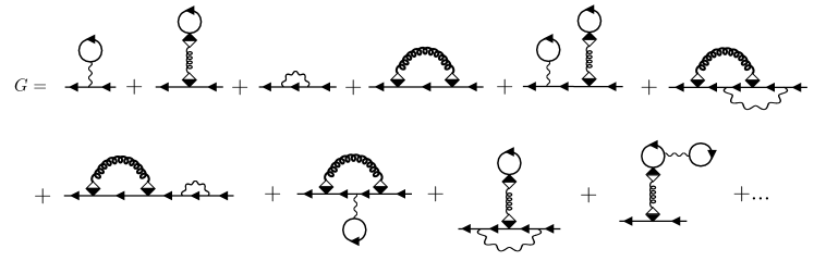
Figure 2: Low-order diagrams in the expansion of the interacting electronic Green’s function $G$.

Diagrammatic expansion for $G$.– In Fig. 2 we show a few low-order Feynman diagrams for $G$. The Feynman rules to convert the diagrams into a mathematical expression are

• Number all vertices and assign an interaction $v(i;j)$ to a wiggly line connecting $i$ and $j$, an $e$-$ph$ coupling $g(i;j^{\ast})$ to a square with white vertex in $j$ and black vertex $i$, a GF $G_{0}^{s}(i;j^{+})$ to an oriented line from $j$ to $i$, a GF $D_{0}(i,j)$ to a spring connecting $i$ and $j$.

• Integrate over all internal vertices and multiply by $i^{k+p}(-)^{l}$ where $l$ is the number of electronic loops, $k$ is the number of wiggly lines and $2p$ is the number of squares.

There are diagrams (5-th and 7-th diagrams in the second row of Fig. 2) that are one-$G_{0}^{s}$-line reducible, i.e., they can be disconnected into two pieces by cutting an internal $G_{0}^{s}$-line. We define the irreducible self-energy $\Sigma$ as the set of all one-$G_{0}^{s}$-line irreducible diagrams with the external (ingoing and outgoing) $G_{0}^{s}$-line removed. Then $G$ can be written as a geometric series

$$G=G_{0}^{s}+G_{0}^{s}\Sigma G_{0}^{s}+G_{0}^{s}\Sigma G_{0}^{s}\Sigma G_{0}^{s}+\ldots=G_{0}^{s}+G_{0}^{s}\Sigma G.$$ (93)

Each product in this formula stand for a space-spin-time convolution. The self-energy $\Sigma=\Sigma[G_{0}^{s},D_{0},v,g]$ is an infinite sum of irreducible diagrams with $G_{0}^{s}$-lines and $D_{0}$-lines connected through $v$ and $g$.

Among the self-energy diagrams there are some with self-energy insertions, i.e., diagrams that can be disconnected into two pieces by cutting two $G_{0}^{s}$-lines. We say that a diagram is $G$-skeletonic if it does not contain self-energy insertions. Then the full set of $\Sigma$-diagrams is obtained by dressing the $G_{0}^{s}$-lines of the skeleton diagrams with all possible self-energy insertions. This amounts to evaluate the skeleton diagrams with the interacting GF $G$ instead of $G_{0}^{s}$ Stefanucci and van Leeuwen (2013). Denoting by $\Sigma_{1\rm skel}$ the sum of only $G$-skeleton diagrams we can write

$$\Sigma=\Sigma[G_{0}^{s},D_{0},v,g]=\Sigma_{1\rm skel}[G,D_{0},v,g].$$ (94)

Figure 3: Low-order diagrams in the expansion of the interacting phononic Green’s function $\widetilde{D}$.

Diagrammatic expansion for $\widetilde{D}$.– Let us now consider the one-particle phononic GF $\widetilde{D}$. Expanding $G_{0,n}$ and $D_{0,m}$ in Eq. (91) according to Wick’s theorem and representing every term of the expansion with a diagram we obtain the diagrammatic expansion of $\widetilde{D}$. The Feynman rules for the $\widetilde{D}$-diagrams are the same as for the $G$ diagrams. In Fig. 3 we illustrate a few low-order diagrams.

Figure 4: Resummation of the tadpole diagrams.

We can clearly distinguish the diagrams belonging to class (c2). These are the double tadpole diagrams (see 2-nd, 4-th, 5-th and 6-th diagrams of Fig. 3). The single tadpole diagrams constitute the diagrammatic expansion of the half-particle phononic GF $\widetilde{D}_{1/2}=\varphi/i^{1/2}$. In Fig. 4 we show the diagrammatic expansion of $\varphi$. The full set of diagrams can be easily summed up, see r.h.s. in Fig. 4 where the oriented double line denotes the interacting GF $G$. The Feynman rules for the $\varphi$-diagrams are the same as for the $G$ diagrams and $D$ diagrams except that the prefactor is $i^{k+p+1}(-)^{l+1}$ where $l$ is the number of electronic loops, $k$ is the number of wiggly lines and $2p+1$ is the number of squares, see Eq. (92). We thus have

$$\varphi(a)=i\int d\tilde{1}d\bar{1}D_{0}(a,\tilde{1})g(\bar{1};\tilde{1}^{\ast})G(\bar{1},\bar{1}^{+}),$$ (95)

a result that could alternatively be found by direct integration of the equation of motion Eq. (52) after taking into account that the electronic density $n(1)=-iG(1;1^{+})$. We can therefore write the expansion of $\widetilde{D}$ as

$$\widetilde{D}(a,b) =\widetilde{D}_{1/2}(a)\widetilde{D}_{1/2}(b)$$

$$+\left[D_{0}+D_{0}\Pi D_{0}+D_{0}\Pi D_{0}\Pi D_{0}+...\right](a,b),$$ (96)

in which the products in this formula stand for momentum-mode-component-time convolutions. The phononic self-energy $\Pi=\Pi[G_{0}^{s},D_{0},v,g]$ is the set of all diagrams that, after the removal of the ingoing and outgoing $D_{0}$-lines, cannot be cut into two pieces by cutting an internal $D_{0}$-line (one-$D_{0}$-line irreducible diagrams).

The phononic Green’s function $\widetilde{D}(a,b)$ does not fulfill a Dyson equation but the fully connected phononic GF

$$D(a,b) \equiv\widetilde{D}(a,b)-\widetilde{D}_{1/2}(a)\widetilde{D}_{1/2}(b)$$

$$=\widetilde{D}(a,b)-\frac{1}{i}\varphi(a)\varphi(b)$$ (97)

does. The GF $D(a,b)$ can alternatively be written in terms of the fluctuation operators $\Delta\hat{\varphi}(a)\equiv\hat{\varphi}(a)-\varphi(a)=\hat{\phi}(a)-\phi(a)=\Delta\hat{\phi}(a)$. We have

$$D(a,b) =\frac{1}{i}{\rm Tr}\Big{[}\hat{\rho}\;\mbox{$\mathcal{T}$}\Big{\{}\Delta\hat{\varphi}_{H}(a)\Delta\hat{\varphi}_{H}(b)\Big{\}}\Big{]}$$

$$=\frac{1}{i}{\rm Tr}\Big{[}\hat{\rho}\;\mbox{$\mathcal{T}$}\Big{\{}\Delta\hat{\phi}_{H}(a)\Delta\hat{\phi}_{H}(b)\Big{\}}\Big{]}.$$ (98)

The GF $D(a,b)$ fulfills a Dyson equation since

$$D(a,b) =\left[D_{0}+D_{0}\Pi D_{0}+D_{0}\Pi D_{0}\Pi D_{0}+...\right](a,b)$$

$$=D_{0}(a,b)+(D_{0}\Pi D)(a,b).$$ (99)

Like for the electronic Green’s function we can express the phononic self-energy in terms of $G$-skeleton diagrams. We remove all diagrams with $\Sigma$-insertions inside the $\Pi$-diagrams and then replace $G_{0}^{s}$ by the full GF $G$, thus obtaining the functional $\Pi_{1\rm skel}$:

$$\Pi=\Pi[G_{0}^{s},D_{0},v,g]=\Pi_{1\rm skel}[G,D_{0},v,g].$$ (100)

The topological idea of the skeletonic expansion in $G$ is completely general and it can be extended to the phononic GF $D$ and the screened Coulomb interaction $W$. This is done in the next section.

IX From the skeletonic expansion in $D$ and $W$ to the Hedin-Baym equations

Skeletonic expansion in $D$.– If we remove all phononic self-energy insertions inside the $\Pi_{1\rm skel}$-diagrams and then replace $D_{0}$ with $D$ we can write

$$\Pi=\Pi_{1\rm skel}[G,D_{0},v,g]=\Pi_{2\rm skel}[G,D,v,g].$$ (101)

Here $\Pi_{2\rm skel}$ contains all doubly skeletonic self-energy diagrams, i.e., all those diagrams that do not contain either $\Sigma$-insertions or $\Pi$-insertions. Examples of $\Pi_{2\rm skel}$-diagrams are shown in Fig. 5 (top) where the double spring represents $D$.

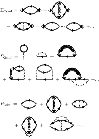
Figure 5: Expansion of the phononic (top) and electronic (middle) self-energies and of the polarization (bottom) in $G$-skeleton diagrams and $D$-skeleton diagrams.

A similar procedure can be applied to the electronic self-energy except that for $\Sigma$ we must exclude the time-local diagrams. In fact, a $\Pi$-insertion is here equivalent to a $\Sigma$-insertion and it would therefore lead to a double counting. Therefore

$$\Sigma=\Sigma_{1\rm skel}[G,D_{0},v,g]=\Sigma_{\rm Eh}[G,D_{0},g]+\Sigma_{2\rm skel}[G,D,v,g],$$ (102)

where $\Sigma_{\rm Eh}$ is the self-energy in the second diagram of Fig. 2 with $G_{0}^{s}\to G$. Using the Feynman rules

$$\Sigma_{\rm Eh}(1;2) =-i\delta(1;2)\!\int\!\!d\tilde{1}d\tilde{2}d\bar{1}\,g(1;\tilde{1}^{\ast})$$

$$\quad\quad\quad\quad\quad\times D_{0}(\tilde{1},\tilde{2})g(\bar{1};\tilde{2}^{\ast})G(\bar{1};\bar{1}^{+})$$

$$=-\delta(1;2)\int d\tilde{1}\,g(1;\tilde{1}^{\ast})\varphi(\tilde{1}),$$ (103)

where in the last equality we use Eq. (95). The self-energy $\Sigma_{\rm Eh}$ is known as the Ehrenfest self-energy. The Ehrenfest approximation consists in including the phononic feedback on the electrons through $\Sigma_{\rm Eh}$, the electronic feedback on the phonons through the density, see Eq. (95), and in setting $\Pi=0$. In this approximation the nuclei are therefore treated as classical particles since they are described in terms of displacements and momenta only, i.e., the components of $\varphi$ Horsfield et al. (2004a, b); Li et al. (2005); Verdozzi et al. (2006); Galperin et al. (2007, 2008); Dundas et al. (2009); Hussein et al. (2010); Lü et al. (2010); Bode et al. (2011); Hübener et al. (2018). The importance of the Ehrenfest diagram in the description of polarons has been pointed out in Refs. Galperin et al. (2008); Lafuente-Bartolome et al. (2022). We expect that the Ehrenfest diagram is also crucial to capture the phonon-induced coherent modulation of the excitonic resonances Trovatello et al. (2020). Examples of $\Sigma_{2\rm skel}$ diagrams are shown in Fig. 5 (middle).

Skeletonic expansion in $W$.– Like in the case of only electrons Hedin (1965) we can further reduce the number of diagrams by removing all those diagrams containing a polarization insertion, which we here define as a piece that can be cut away by cutting two $v$-lines and at the same time it does not break into two disjoint pieces by cutting one $v$-line or one $D$-line, an example is the 5-th diagram in the $\Sigma$-expansion of Fig. 5 (middle). The polarization diagrams are therefore one-$v$-line irreducible and one-$D$-line irreducible. To the best of our knowledge the diagrammatic definition of the polarization $P$ in systems of electrons and phonons is given here for the first time. In Fig. 5 (bottom) we show a few low-order diagrams for $P=P_{2\rm skel}[G,D,v,g]$ which are both $G$-skeletonic and $D$-skeletonic. The polarization $P$ contains both electronic and phononic contributions. For later purposes we also define the one-$v$-line irreducible, one-$D$-line irreducible and two-$G$-lines reducible kernel $\tilde{K}_{r}$ from the polarization according to

$$\raisebox{-6.0pt}{\includegraphics[width=182.1196pt]{ptildektilde.pdf}}\;\;,$$ (104)

where the dark-grey bubble represents $P$ and the square grid represents $\tilde{K}_{r}(\bar{1},\bar{2};\bar{3},\bar{4})=\tilde{K}_{r}(\bar{2},\bar{1};\bar{4},\bar{3})$. This is the same definition used in the case of systems of only electrons. In fact, the so called vertex function $\Gamma=\delta-\tilde{K}_{r}GG$ relates to $P$ through the well known formula $P=-iGG\Gamma$ (the factor of “ $i$ ” in the second diagram of Eq. (104) comes from the Feynman rules for the polarization diagrams). Following the same strategy as in Ref. Stefanucci and van Leeuwen (2013) one can show that the kernel $\tilde{K}_{r}$ satisfies the Bethe-Salpeter equation

$$\raisebox{-6.0pt}{\includegraphics[width=195.12767pt]{BSE-kernel.pdf}}\;\;,$$ (105)

where the kernel $\tilde{K}$, represented by the square with only vertical lines, is one-$v$-line irreducible, one-$D$-line irreducible and two-$G$-lines irreducible.

From the polarization diagrams we can construct the dynamically screened interaction in the usual manner

$$\raisebox{-6.0pt}{\includegraphics[width=173.44534pt]{Welect.pdf}}\;\;.$$ (106)

We say that a diagram is $W$-skeletonic if it does not contain $P$-insertions. Then the desired expression for $\Pi$ and $\Sigma$ is obtained by discarding all those diagrams which are not $W$-skeletonic, and then replacing $v$ with $W$.

Phononic self-energy.– For the phononic self-energy we get

$$\Pi=\Pi_{2\rm skel}[G,D,v,g]=\Pi_{3\rm skel}[G,D,W,g],$$ (107)

where $\Pi_{3\rm skel}$ is the sum of all the triply skeletonic self-energy diagrams, i.e., all those diagrams that do not contain either $\Sigma$-insertions, $\Pi$-insertions or $P$-insertions. In Fig. 6 (top) we show a few low-order diagrams of the triply skeletonic expansion for $\Pi_{3\rm skel}$.

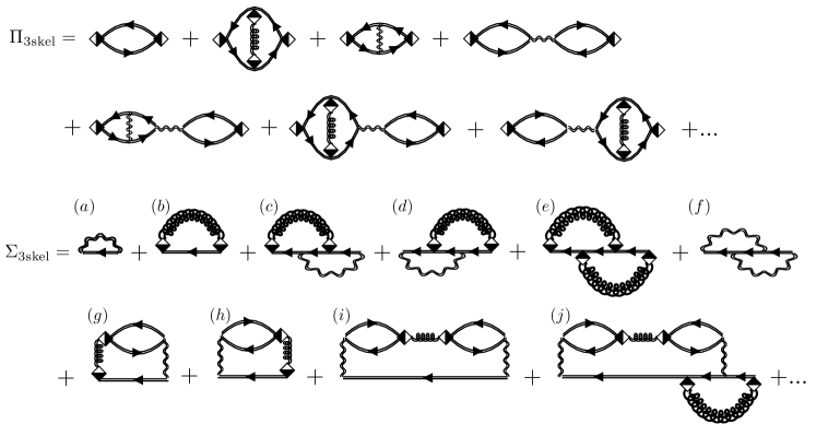
Figure 6: Expansion of the phononic (top) and electronic (bottom) self-energy in $G$-skeleton diagrams, $D$-skeleton diagrams and $W$-skeleton diagrams. To facilitate the discussion in the main text we have labelled the $\Sigma$-diagrams.

They are one-$G$-line irreducible, one-$D$-line irreducible and two-$W$-lines irreducible, i.e., they cannot break into disjoint pieces by cutting two $W$-lines for otherwise they would contain a polarization insertion. We then have either one-$W$-line reducible diagrams or one-$W$-line irreducible diagrams. We can write $\Pi$ in a compact form using the polarization $P$. We define the dressed (or screened) $e$-$ph$ coupling $g^{d}$ as

$$=g+WPg\;\;,\quad\quad\quad\quad\quad\;$$ (108)

In terms of the dressed $e$-$ph$ coupling the phononic self-energy can be represented as

$$\raisebox{-6.0pt}{\includegraphics[width=86.72267pt]{Piwithdressedvertex.pdf}}\;\;,$$

$$=gPg^{d}\;\;,\quad\quad\quad\quad\quad\quad$$ (109)

in agreement with the field-theoretic approach Giustino (2017). We see from this expression that one $e$-$ph$ coupling is bare whereas the other is dressed. As pointed out in Refs. Giustino (2017); Marini (2023) this structure has to be properly taken into account for the calculation of phonons, although a symmetrized form where both $e$-$ph$ couplings are dressed has been shown to give satisfactory results Calandra et al. (2010), which has been attributed to error cancellations Berges et al. (2022).

Electronic self-energy.– For the electronic self-energy $\Sigma$ the only diagram for which we should not proceed with the replacement is the Hartree diagram [first diagram in Fig. 5 (middle)] since here every polarization insertion is equivalent to a self-energy insertion, hence $v\rightarrow W$ would lead to a double counting. Therefore

$$\Sigma =\Sigma_{\rm Eh}[G,D_{0},g]+\Sigma_{2\rm skel}[G,D,v,g]$$

$$=\Sigma_{\rm Eh}[G,D_{0},g]+\Sigma_{\rm H}[G,v]+\Sigma_{3\rm skel}[G,D,W,g],$$ (110)

where $\Sigma_{\rm H}$ is the Hartree diagram. The self-energy $\Sigma_{3\rm skel}$ is also called the exchange-correlation (xc) self-energy. Henceforth we shall equivalently write $\Sigma_{3\rm skel}$ or $\Sigma_{\rm xc}$. The diagrammatic expansion of the xc self-energy plays a crucial role in diagrammatic theory since the Bethe-Salpeter kernel $\tilde{K}(1,2;3,4)=-\delta\Sigma_{\rm xc}(1;3)/\delta G(4;2)$, see Eq. (105). This statement can be proven along the same lines as in Ref. Stefanucci and van Leeuwen (2013). We illustrate in Fig. 6 (bottom) a few low-order diagrams of the triply skeletonic expansion of $\Sigma_{3\rm skel}$. Diagrams like the last two in the figure must be included since by cutting the two $W$-lines we get a piece that is neither a polarization insertion nor a $\Pi$-insertion.

Like the phononic self-energy also the electronic self-energy $\Sigma$ can be written in a compact form using the polarization $P$, or more precisely the kernel $\tilde{K}_{r}$. Let us consider the admissible “effective” interactions that can sprout from, e.g., the left vertex of $\Sigma_{\rm xc}$. Keeping an eye on Fig. 6 (bottom) we realize that we can have $W$, see diagrams $(a)$, $(d)$ and $(f)$, and $[gDg]$, see diagrams $(b)$, $(c)$ and $(e)$. We can also have $WP[gDg]$, see diagram $(h)$, but we cannot have $WPW$ since the corresponding diagram would contain a $P$-insertion. We can further have $[gDg]PW$, see diagram $(g)$, but we cannot have $[gDg]P[gDg]$ since the corresponding diagram would contain a $\Pi$-insertion. We can finally have $WP[gDg]PW$, see diagrams $(i)$ and $(j)$. All other structures are non-skeletonic: $WP[gDg]P[gDg]$ and $[gDg]PWP[gDg]$ contain a $\Pi$-insertion whereas $[gDg]PWPW$ contains a polarization insertion. We conclude that the total “effective” interaction sprouting from the left vertex is

$$\widetilde{W} =W\!+gDg+W\!PgDg+gDgPW+W\!PgDgPW$$

$$=W+(g+WPg)D(g+gPW)$$

$$=W+g^{d}Dg^{d}.$$ (111)

To make these graphical considerations rigorous we define the phonon-mediated $e$-$e$ interaction from the dressed $e$-$ph$ coupling according to

$$\raisebox{-6.0pt}{\includegraphics[width=130.08731pt]{Wdispl.pdf}}\;\;,$$ (112)

or in formulas

$$W_{ph}(1;2)=\int d\tilde{1}d\tilde{2}\,g^{d}(1;\tilde{1}^{\ast})D(\tilde{1},\tilde{2})g^{d}(2;\tilde{2}^{\ast}),$$ (113)

and the total screened interaction $\widetilde{W}\equiv W+W_{ph}$ according to

$$\raisebox{-6.0pt}{\includegraphics[width=195.12767pt]{Wtot.pdf}}\;\;,$$ (114)

or in formulas

$$\widetilde{W}(1;2)=W(1;2)+\,W_{ph}(1;2).$$ (115)

The total electronic self-energy can then be written as

$$\raisebox{-6.0pt}{\includegraphics[width=195.12767pt]{SigmawithWtotandGamma.pdf}}\;\;.$$ (116)

$\begin{array}[]{c}\vspace{-1.2cm}\hfil\\ G=G^{s}_{0}+G^{s}_{0}\Sigma G\end{array}$
$\begin{array}[]{c}\vspace{-1.4cm}\hfil\\ D=D_{0}+D_{0}\Pi D\end{array}$
$\begin{array}[]{l}\vspace{-1.cm}\\ \Sigma=\Sigma_{\rm Eh}+\Sigma_{\rm H}+iG\widetilde{W}(\delta-GG\tilde{K}_{r})\\ \end{array}$
$\begin{array}[]{c}\vspace{-1.4cm}\hfil\\ \Pi=gPg^{d}\end{array}$
$\begin{array}[]{c}\vspace{-1.6cm}\hfil\\ \widetilde{W}\equiv W+g^{d}Dg^{d}\end{array}$
$\begin{array}[]{c}\vspace{-1.6cm}\hfil\\ W=(\delta+WP)v\end{array}$
$\begin{array}[]{c}\vspace{-1.3cm}\hfil\\ P=-iGG(\delta-\tilde{K}_{r}GG)\end{array}$
$\begin{array}[]{c}\vspace{-1.7cm}\hfil\\ g^{d}=(\delta+WP)g\end{array}$
$\begin{array}[]{c}\vspace{0.cm}\hfil\\ \tilde{K}_{r}=-\frac{\mbox{$\delta\Sigma_{\rm xc}$}}{\mbox{$\delta G$}}(\delta-GG\tilde{K}_{r})\end{array}$	$\begin{array}[]{c}\vspace{0.1cm}\hfil\\ \includegraphics[width=199.16928pt]{hedineb8.pdf}\end{array}$

Table 1: Mathematical expression (left column) and diagrammatic representation (right column) of the Hedin-Baym equations for systems of interacting electrons and phonons.

Hedin-Baym equations.– We summarize in Table 1 the fundamental equations that relate the various many-body quantities, i.e., $G$, $D$, $\Sigma$, $\Pi$, $\widetilde{W}$, $W$, $P$, $g^{d}$ and $\tilde{K}_{r}$. We here align with Ref. Giustino (2017) and call to the full set of equations in Table 1 the Hedin-Baym equations for electrons and phonons. The Hedin-Baym equations provide a closed system of equations for any diagrammatic approximation to the xc self-energy through the irreducible kernel $\tilde{K}=\delta\Sigma_{\rm xc}/\delta G$. They are equations on the contour and can therefore be used to study systems in equilibrium at any temperature as well as systems driven away from equilibrium by external fields. For systems in equilibrium at zero temperature the adiabatic assumption in conjunction with the assumption of a nondegenerate ground state allows for deforming the contour into a single branch going from $-\infty$ to $+\infty$, i.e., the real axis Stefanucci and van Leeuwen (2013). In this case the contour Green’s functions become the more familiar time-ordered Green’s functions and the Hedin-Baym equations reduce to those presented in Ref. Giustino (2017). We emphasize that no such shortcut is possible at finite temperature. One way to avoid the use of the $L$-shaped contour for equilibrium systems at finite temperature is the analytic continuation (from Matsubara to retarded to time-ordered) which may however be rather cumbersome in the presence of singularities or branch cuts, although notable progresses have been recently made Fei et al. (2021a, b); Nogaki and Shinaoka (2023).

Like for the Hedin equations for only electrons the Hedin-Baym equations can be iterated to obtain an expansion of $\Sigma$ and $\Pi$ in terms of $G$, $W$, $D$ and $g$. If we start with $\tilde{K}_{r}=0$, hence

$$P\simeq\chi^{0}=-iGG,$$ (117)

the electronic self-energy $\Sigma$ is approximated by

$$\Sigma=\Sigma_{\rm Eh}+\Sigma_{\rm H}+\Sigma_{\rm GW}+\Sigma_{\rm FM},$$ (118)

where $\Sigma_{\rm GW}=iGW$ is the well known $GW$ self-energy with RPA screened interaction $W=v+v\chi^{0}W$, and

$$\Sigma_{\rm FM}=ig^{d}GDg^{d}$$ (119)

is the so called Fan-Migdal self-energy Fan (1951); Migdal (1958) with dressed electron-phonon coupling

$$g^{d}=(\delta+W\chi^{0})g.$$ (120)

The phononic self-energy for $\tilde{K}_{r}=0$ is simply

$$\Pi=g\,\chi^{0}\,g^{d}=g(\chi^{0}+\chi^{0}W\chi^{0})g.$$ (121)

We remark that the response function $\chi^{0}$ appearing in $W$ and $\Pi$ cannot, in general, be built with a quasi-particle GF $G$ since both $\Sigma_{\rm GW}$ and $\Sigma_{\rm FM}$ are non-local in time. Although the time-local Coulomb-hole plus Screened Exchange (COH-SEX) version of $\Sigma_{\rm GW}$ often provides a good compromise in the trade-off between accuracy and computational cost we are not aware of a similar time-local version of $\Sigma_{\rm FM}$. In Section X we show that the approximation in Eqs. (118) and (121) is conserving, i.e., the resulting GF satisfy all fundamental conservation laws.

Inserting an approximation for the self-energies $\Sigma$ and $\Pi$ into the Dyson equations $G=G_{0}^{s}+G_{0}^{s}\Sigma G$ and $D=D_{0}+D_{0}\Pi D$ we obtain a closed system of equations for $G$ and $D$ for any $G_{0}^{s}$ and $D_{0}$. The GF $D_{0}$ depends only on the parameters of the Hamiltonian, see also Appendix A, whereas the GF $G_{0}^{s}$ depends also on the nuclear displacements through $h^{s}$. The Hedin-Baym equations must therefore be coupled to Eq. (95).

The Hedin-Baym equations can alternatively be derived using the field-theoretic approach Giustino (2017); van Leeuwen (2004); de Melo and Marini (2016); Härkönen et al. (2020); Marini (2023). We emphasize that the field-theoretic approach prescinds from any diagrammatic notion, i.e., it does not tell us how to expand the various many-body quantities diagrammatically.

X Equations of motion for the Green’s functions

An alternative route to solving the Hedin-Baym equations is the solution of the equations of motion for the GF. This second route is more convenient for systems at finite temperature or out of equilibrium. We here consider the self-energies as functionals of $G$ and $D$ (doubly skeletonic expansion). Using the equation of motion for $D_{0}$, see Eq. (67), and for $G_{0}^{s}$, see Eq. (71), we can convert the Dyson equations Eqs. (93) and (99) into integro-differential equations on the contour

$$\int d\bar{1}\;\overrightarrow{G}_{0}^{-1}(1;\bar{1})G(\bar{1};2) =\delta(1;2)+\int d\bar{1}\,\Sigma(1;\bar{1})G(\bar{1};2),$$ (122a)

$$\int d\tilde{1}\;\overrightarrow{D}_{0}^{-1}(1,\tilde{1})D(\tilde{1},2^{\ast}) =\delta(1,2)+\int d\tilde{1}\,\Pi(1^{\ast},\tilde{1})D(\tilde{1},2^{\ast}).$$ (122b)

Equation of motion for $G$.– We separate the electronic self-energy into a time-local (singular) contribution $\Sigma^{\delta}(1;2)\propto\delta(z_{1},z_{2})$ and a rest $\Sigma_{\rm c}(1;2)$ which is called the correlation self-energy:

$$\Sigma=\Sigma^{\delta}+\Sigma_{\rm c}.$$ (123)

The singular contribution is given by the sum of the Hartree-Fock (HF) self-energy $\Sigma_{\rm HF}(1;2)=\delta(z_{1},z_{2})V_{\rm HF}({\mathbf{x}}_{1},{\mathbf{x}}_{2},z_{1})$, with $V_{\rm HF}$ the spatially nonlocal HF potential, and the Ehrenfest self-energy $\Sigma_{\rm Eh}(1;2)=-\delta(1;2)\sum_{{\mathbf{q}}\nu}\mbox{\boldmath$g$}_{{\mathbf{q}}\nu}^{{\dagger}}({\mathbf{r}}_{1},z_{1})\cdot\mbox{\boldmath$\varphi$}_{{\mathbf{q}}\nu}(z_{1})$, see Eq. (103). Then Eq. (122a) can be rewritten as

$$\int d\bar{1}\;\overrightarrow{G}_{\rm mf}^{-1}(1;\bar{1})G(\bar{1};2) =\delta(1;2)+\int d\bar{1}\,\Sigma_{\rm c}(1;\bar{1})G(\bar{1};2),$$ (124)

where the mean-field operator $\overrightarrow{G}_{\rm mf}^{-1}(1;2)\equiv\overrightarrow{G}_{0}^{-1}(1;2)-\Sigma^{\delta}(1;2)$. Taking into account the definition of $\overrightarrow{G}_{0}^{-1}$ in Eq. (58b) and the definition of the shifted one-particle Hamiltonian $h^{s}$ in Eq. (55) one finds

$$\overrightarrow{G}_{\rm mf}^{-1}(1;2) =\Big{[}i\frac{d}{dz_{1}}-h(\mbox{\boldmath$\nabla$},{\mathbf{r}},z)+\!\sum_{{\mathbf{q}}\nu}g_{-{\mathbf{q}}\nu}({\mathbf{r}},z)U_{{\mathbf{q}}\nu}(z)\Big{]}\delta(1;2)$$

$$-V_{\rm HF}({\mathbf{x}}_{1},{\mathbf{x}}_{2},z_{1})\delta(z_{1},z_{2})$$ (125)

where we also take into account Eq. (51) and the fact that electrons are coupled to the phonons only through the displacements, see Eq. (44f).

For simplicity we specialize the discussion to the relevant case of external perturbations that do not break the lattice periodicity of the crystal, albeit the developed formalism is far more general. Let us write the coordinates ${\mathbf{r}}=(x,y,z)$ of any point in space as the sum of the vector ${\mathbf{R}}^{0}_{{\mathbf{n}}}$ of the unit cell the point ${\mathbf{r}}$ belongs to and a displacement ${\mathbf{u}}$ spanning the unit cell centered at the origin, i.e., ${\mathbf{r}}={\mathbf{R}}^{0}_{{\mathbf{n}}}+{\mathbf{u}}$. We introduce a generic one-electron Bloch basis, e.g., the Kohn-Sham basis, $\Psi_{{\mathbf{k}}\mu}({\mathbf{x}}={\mathbf{r}}\sigma)=e^{i{\mathbf{k}}\cdot{\mathbf{n}}}u_{{\mathbf{k}}\mu}({\mathbf{u}}\sigma)/\sqrt{N}$ where the vector ${\mathbf{k}}$ takes the same values as the vector ${\mathbf{q}}$ defined below Eqs. (25). The wavefunctions $\Psi_{{\mathbf{k}}\mu}({\mathbf{x}})$ can be thought of as the one-electron eigenfunctions in some potential, e.g., the Kohn-Sham potential, with the periodicity of our lattice; hence the index $\mu$ can be thought of as a band index. The matrix element of any two-point correlator with the same periodicity, calculated by sandwiching with $\Psi^{\ast}_{{\mathbf{k}}_{1}\mu_{1}}$ and $\Psi_{{\mathbf{k}}_{2}\mu_{2}}$, is proportional to $\delta_{{\mathbf{k}}_{1},{\mathbf{k}}_{2}}$. If we then multiply Eq. (124) by $\Psi^{\ast}_{{\mathbf{k}}\mu_{1}}({\mathbf{x}}_{1})$ from the left and by $\Psi_{{\mathbf{k}}\mu_{2}}({\mathbf{x}}_{2})$ from the right and we integrate over ${\mathbf{x}}_{1}$ and ${\mathbf{x}}_{2}$ we find (in matrix form)

$$\Big{[}i\frac{d}{dz_{1}}-h_{\rm HF}({\mathbf{k}},z_{1}) +\sum_{\nu}\tilde{g}_{\nu}({\mathbf{k}},z_{1})U_{{\mathbf{0}}\nu}(z_{1})\Big{]}G_{{\mathbf{k}}}(z_{1},z_{2})$$

$$=\delta(z_{1},z_{2})+\!\!\int_{\gamma}\!d\bar{z}\,\Sigma_{\rm c,{\mathbf{k}}}(z_{1},\bar{z})G_{{\mathbf{k}}}(\bar{z},z_{2}),$$ (126)

where

$$h_{\rm HF,\mu_{1}\mu_{2}}({\mathbf{k}},z_{1})=\int d{\mathbf{x}}_{1}d{\mathbf{x}}_{2}\Psi^{\ast}_{{\mathbf{k}}\mu_{1}}({\mathbf{x}}_{1})$$

$$\times\Big{(}h(\mbox{\boldmath$\nabla$}_{1},{\mathbf{r}}_{1},z_{1})\delta({\mathbf{x}}_{1}-{\mathbf{x}}_{2})+V_{\rm HF}({\mathbf{x}}_{1},{\mathbf{x}}_{2},z_{1})\Big{)}\Psi_{{\mathbf{k}}\mu_{2}}({\mathbf{x}}_{2})$$ (127)

and the like for the matrix elements $G_{{\mathbf{k}}\mu_{1}\mu_{2}}$ and $\Sigma_{\rm c,{\mathbf{k}}\mu_{1}\mu_{2}}$. The term proportional to $U_{{\mathbf{0}}\nu}$ in Eq. (126) originates from

$$\int d{\mathbf{x}}_{1}\Psi^{\ast}_{{\mathbf{k}}\mu_{1}}({\mathbf{x}}_{1})g_{-{\mathbf{q}}\nu}({\mathbf{r}}_{1},z_{1})\Psi_{{\mathbf{k}}\mu_{2}}({\mathbf{x}}_{1})=\delta_{{\mathbf{q}},{\mathbf{0}}}\,\tilde{g}_{\nu,\mu_{1}\mu_{2}}({\mathbf{k}},z_{1}),$$ (128)

which implicitly defines the matrix $\tilde{g}_{\nu}({\mathbf{k}},z_{1})$. The Kronecker-delta on the r.h.s. follows from the property Eq. (24) of the $e$-$ph$ coupling which in turns implies [see Eq. (30)]

$$g_{-{\mathbf{q}}\nu}({\mathbf{r}}+{\mathbf{R}}^{0}_{{\mathbf{n}}},z)=e^{-i{\mathbf{q}}\cdot{\mathbf{n}}}g_{-{\mathbf{q}}\nu}({\mathbf{r}},z).$$ (129)

Equation (126) is consistent with the fact that the only displacements activated by an external perturbation preserving the lattice periodicity are the uniform ones. Of course, this does not mean that only zero-momentum phonons are emitted or absorbed, see below.

Equation of motion for displacements and momenta.– Writing Eq. (48) component-wise we find

$$\frac{dP_{{\mathbf{q}}\nu}(z)}{dz} =\int\!d{\mathbf{x}}\,g_{{\mathbf{q}}\nu}({\mathbf{r}},z)\Delta n({\mathbf{x}},z)-\sum_{\nu^{\prime}}K_{\nu\nu^{\prime}}({\mathbf{q}},z)U_{{\mathbf{q}}\nu^{\prime}}(z),$$ (130a)

$$\frac{dU_{{\mathbf{q}}\nu}(z)}{dz} =P_{{\mathbf{q}}\nu}(z),$$ (130b)

where $P_{{\mathbf{q}}\nu}$ is the average of $\hat{P}_{{\mathbf{q}}\nu}=\hat{\phi}^{2}_{{\mathbf{q}}\nu}$ and $U_{{\mathbf{q}}\nu}$ is the average of $\hat{U}_{{\mathbf{q}}\nu}=\hat{\phi}^{1}_{{\mathbf{q}}\nu}$. The first of these equations agrees with Eq. (22) whereas the second equation establishes that $P_{{\mathbf{q}}\nu}$ is the conjugate momentum of $U_{{\mathbf{q}}\nu}$. Alternatively, $U_{{\mathbf{q}}\nu}$ and $P_{{\mathbf{q}}\nu}$ can be calculated from $\phi^{i}_{{\mathbf{q}}\nu}=\varphi^{i}_{{\mathbf{q}}\nu}+s^{i}_{{\mathbf{q}}\nu}$, see Eq. (51), where $\varphi^{i}_{{\mathbf{q}}\nu}$ is given by Eq. (95). It is straightforward to find

$$U_{{\mathbf{q}}\nu}(z) =-\sum_{\nu^{\prime}}\int d\bar{{\mathbf{x}}}d\bar{z}\,D_{0,{\mathbf{q}}\nu\nu^{\prime}}^{11}(z,\bar{z})\,g_{{\mathbf{q}}\nu^{\prime}}(\bar{{\mathbf{r}}})\Delta n(\bar{{\mathbf{x}}},\bar{z}),$$ (131a)

$$P_{{\mathbf{q}}\nu}(z) =-\sum_{\nu^{\prime}}\int d\bar{{\mathbf{x}}}d\bar{z}\,D_{0,{\mathbf{q}}\nu\nu^{\prime}}^{21}(z,\bar{z})g_{{\mathbf{q}}\nu^{\prime}}(\bar{{\mathbf{r}}})\Delta n(\bar{{\mathbf{x}}},\bar{z}),$$ (131b)

where have taken into account Eq. (68). In equilibrium $\Delta n=0$ and therefore $U_{{\mathbf{q}}\nu}=P_{{\mathbf{q}}\nu}=0$. Under the hypothesis that the external perturbation does not break the lattice periodicity we also have $U_{{\mathbf{q}}\nu}(z)=P_{{\mathbf{q}}\nu}(z)=0$ for all ${\mathbf{q}}\neq 0$.

Equation of motion for $D$.– We have already observed that $D_{0}(1,2)\propto\delta_{{\mathbf{q}}_{1},-{\mathbf{q}}_{2}}$, see Eq. (68). Let us now investigate the mathematical structure of the phononic self-energy. Combining Eqs. (108) and (109) we can write

$$\Pi=gP(g+WPg)=g(P+PWP)g=g\chi g$$ (132)

where $\chi=P+PWP=P+Pv\chi$ is the density-density response function. Spelling out the space-spin-time convolutions

$$\Pi(1,2) =\Pi({\mathbf{q}}_{1}\nu_{1},i_{1},z_{1},{\mathbf{q}}_{2}\nu_{2},i_{2},z_{2})=\delta_{i_{1},1}\delta_{i_{2},1}\int\!d\bar{{\mathbf{x}}}_{1}d\bar{{\mathbf{x}}}_{2}$$

$$\times\,g_{-{\mathbf{q}}_{1}\nu_{1}}(\bar{{\mathbf{r}}}_{1},z_{1})\chi(\bar{{\mathbf{x}}}_{1},z_{1};\bar{{\mathbf{x}}}_{2},z_{2})g_{-{\mathbf{q}}_{2}\nu_{2}}(\bar{{\mathbf{r}}}_{2},z_{2}).$$ (133)

Working again under the hypothesis that the external perturbation does not break the lattice periodicity $\chi$ is invariant under a simultaneous translations of its spatial coordinates by an arbitrary lattice vector ${\mathbf{R}}^{0}_{{\mathbf{n}}}$. Therefore

$$\Pi(1,2)=\delta_{{\mathbf{q}}_{1},-{\mathbf{q}}_{2}}\Pi_{-{\mathbf{q}}_{1}\nu_{1}\nu_{2}}^{i_{1}i_{2}}(z_{1},z_{2}).$$ (134)

As both $D_{0}(1,2)$ and $\Pi(1,2)$ are proportional to $\delta_{{\mathbf{q}}_{1},-{\mathbf{q}}_{2}}$ the interacting phononic GF $D(1,2)=[D_{0}+D_{0}\Pi D_{0}+D_{0}\Pi D_{0}\Pi D_{0}+\ldots](1,2)$ is also proportional to $\delta_{{\mathbf{q}}_{1},-{\mathbf{q}}_{2}}$, i.e.,

$$D(1,2)=\delta_{{\mathbf{q}}_{1},-{\mathbf{q}}_{2}}D_{{\mathbf{q}}_{1}\nu_{1}\nu_{2}}^{i_{1}i_{2}}(z_{1},z_{2}).$$ (135)

Notice that the phononic self-energy $\Pi$ in the r.h.s. of Eq. (134) is defined with a $-{\mathbf{q}}_{1}$ whereas the phononic GF $D$ in the r.h.s. of Eq. (135) is defined with a $+{\mathbf{q}}_{1}$. These different definitions are chosen to have a more elegant equation of motion. Indeed if we insert these expressions into Eq. (122b) we obtain (in matrix form)

$$\Big{[}i\frac{d}{dz_{1}}\,\alpha -Q({\mathbf{q}},z_{1})\Big{]}D_{{\mathbf{q}}}(z_{1},z_{2})$$

$$=\delta(z_{1},z_{2})+\int_{\gamma}d\tilde{z}\,\Pi_{{\mathbf{q}}}(z_{1},\tilde{z})D_{{\mathbf{q}}}(\tilde{z},z_{2}).$$ (136)

Equations (126), (136) and their counterparts with derivatives with respect to $z_{2}$ along with the equations of motion Eqs. (130) for the displacements and momenta form a closed system of equations for any approximate functional $\Sigma_{{\rm c},2\rm skel}[G,D,v,g]$ and $\Pi_{2\rm skel}[G,D,v,g]$.

XI Conserving approximations

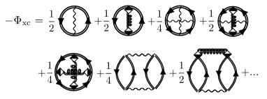
Figure 7: Expansion of the $\Phi_{\rm xc}$ functional in $G$-skeleton diagrams and $D$-skeleton diagrams.

If the self-energies are $\Phi$-derivable Baym (1962); Almbladh et al. (1999); Karlsson and van Leeuwen (2016) then the GF resulting from the solution of Eqs. (126), (136) and (130) satisfy all fundamental conservation laws. To define this properly in the context of electrons and phonons we split off the Ehrenfest-Hartree part of the self-energy like in Eq. (110). In the doubly skeletonic expansion the remainder is the xc self-energy $\Sigma_{\rm xc}[G,D,v,g]=\Sigma_{3\rm skel}[G,D,W,g]$. We then construct the functional $\Phi_{\rm xc}[G,D,v,g]$ using the same rules as for a system of only electrons Stefanucci and van Leeuwen (2013): (i) close each skeleton diagram for $\Sigma_{\rm xc}$ with a $G$-line, thereby producing a set of vacuum diagrams (ii) retain only the topologically inequivalent vacuum diagrams and (iii) multiply every diagram by the corresponding symmetry factor $1/N_{sym}$, where $N_{sym}$ is the number of equivalent $G$ lines yielding the same self-energy diagram by their respective removal. The lowest order diagrams of the expansion are shown in Fig. 7. The additional minus sign is due to the fact that the removal of a $G$-line from a vacuum diagram changes the number of electronic loops by one. By construction the $\Phi_{\rm xc}$ functional has the property that

$$\Sigma_{\rm xc}(1;2) =\frac{\delta\Phi_{\rm xc}}{\delta G(2;1)},$$ (137a)

$$\Pi(1,2) =\left.\frac{\delta\Phi_{\rm xc}}{\delta D(1,2)}\right|_{S},$$ (137b)

where the subscript “ $S$ ” refers to the symmetrized derivative $[\delta/\delta D(1,2)+\delta/\delta D(2,1)]/2$. The Hartree self-energy is obtained from the functional derivative of the Hartree functional

$$\raisebox{-6.0pt}{\includegraphics[width=99.73074pt]{PhiHartree.pdf}}\;\;,$$ (138)

whereas the Ehrenfest self-energy is obtained from the functional derivative of the Ehrenfest functional

$$\raisebox{-6.0pt}{\includegraphics[width=138.76157pt]{PhiEhrenfest.pdf}}\;\;.$$ (139)

Therefore the full self-energy $\Sigma$ is the functional derivative of the $\Phi$-functional defined as

$$\Phi\equiv\Phi_{\rm H}[G,v]+\Phi_{\rm Eh}[G,D_{0},g]+\Phi_{\rm xc}[G,D,v,g].$$ (140)

In most cases we can only deal with approximate functionals. These are obtained by selecting an appropriate subset of $\Phi$-diagrams. We say that the self-energies are $\Phi$-derivable whenever there exists an approximate functional $\Phi$ such that $\Sigma_{\rm xc}$ and $\Pi$ can be written as in Eqs. (137). The $\Phi$-functional is invariant under gauge transformations and contour-time deformations, i.e., $z\to w(z)$ with $w(t_{0})=t_{0}$ and $w(t_{0}-i\beta)=t_{0}-i\beta$, implying the fulfillment of the continuity equation and energy conservation for the GF that satisfy the equations of motion Eqs. (126) and (136) with $\Phi$-derivable self-energies Baym (1962). We mention here that the use of $\Phi$-derivable self-energies evaluated at different input GF still guarantee the satisfaction of all conservation laws provided that they are convoluted with the same input GF Karlsson et al. (2021). In other words, self-consistency is not required for having a conserving theory.

We conclude by observing that the approximation to the self-energies discussed at the end of Section IX (derived by setting $\tilde{K}_{r}=0$ in the Hedin-Baym equations) is $\Phi$-derivable. The diagrams for $\Phi_{\rm xc}$ are those of the GW approximation plus a second infinite sum of ring diagrams in which one $v$-line is replaced by $(gDg)$, see Fig. 8.

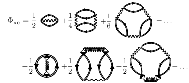
Figure 8: Diagrams of the $\Phi_{\rm xc}$ functional leading to the self-energies Eqs. (118) and (121) through the functional derivatives in Eqs. (137).

XII Kadanoff-Baym equations

Placing the arguments on different branches of the contour and using the Langreth rules Stefanucci and van Leeuwen (2013); l. (1) we can convert the equations of motion Eqs. (126) and (136) into a coupled system of equations for the Keldysh components of $G$ and $D$. These are the Kadanoff-Baym equations (KBE) for systems of electrons and phonons to be solved with KMS boundary conditions. As for the case of only electrons the equations for the Matsubara components decouple. The Matsubara GF $G^{\rm M}$ and $D^{\rm M}$ allow for calculating the initial thermal average of any one-body operator for electrons and of any quadratic operator in the displacements and momenta for the nuclei. The KBE for the GF with times on the horizontal branches (hence the left/right and lesser/greater components) allow for monitoring the system evolution as well as for calculating electronic and phononic spectral functions of the system in any stationary state. As already pointed out below Eqs. (31) we can study how the system responds to different kind of external perturbations, e.g., interaction quenches, laser fields, phonon drivings, etc..

XII.1 Self-consistent Matsubara equations

The preliminary step to solve the equations of motion for the GF consists in solving the Matsubara problem. The Matsubara self-energies do indeed depend only on the Matsubara GF Stefanucci and van Leeuwen (2013) and therefore the equations for the Matsubara components are closed. The Matsubara component of any correlator $X(z_{1},z_{2})$ with arguments on $\gamma$ is defined as $X^{\rm M}(\tau_{1},\tau_{2})\equiv X(z_{1}=t_{0}-i\tau_{1},z_{2}=t_{0}-i\tau_{2})$. The KMS boundary conditions allow for expanding the Matsubara GF and self-energies according

$$X^{\rm M}(\tau_{1},\tau_{2})=\frac{1}{-i\beta}\sum_{m=-\infty}^{\infty}e^{-\omega_{m}(\tau_{1}-\tau_{2})}X^{\rm M}(\omega_{m})$$ (141)

where the Matsubara frequencies $\omega_{m}=2mi\pi/\beta$ for periodic functions like $D$ and $\Pi$ and $\omega_{m}=(2m+1)i\pi/\beta$ for antiperiodic functions like $G$ and $\Sigma_{\rm c}$. Taking into account that along the vertical track $U_{{\mathbf{q}}\nu}=P_{{\mathbf{q}}\nu}=0$ since $\Delta n=0$, see Eq. (131), the equations of motion Eqs. (126) and (136) yield

$$G^{\rm M}_{{\mathbf{k}}}(\omega_{m}) =\frac{1}{\omega_{m}-h_{\rm HF}({\mathbf{k}})-\mu-\Sigma_{\rm c,{\mathbf{k}}}^{\rm M}(\omega_{m})},$$ (142a)

$$D^{\rm M}_{{\mathbf{q}}}(\omega_{m}) =\frac{1}{\omega_{m}\alpha-Q({\mathbf{q}})-\Pi^{\rm M}_{{\mathbf{q}}}(\omega_{m})},$$ (142b)

where $Q({\mathbf{q}})=\left(\begin{array}[]{cc}K({\mathbf{q}})&0\\ 0&1\end{array}\right)$, see Eq. (44c). For any approximation to $\Sigma_{\rm c}[G,D,v,g]$ and $\Pi[G,D,v,g]$ these equations can be solved self-consistently. We recall that $K=K[n^{0}]$ depends on the equilibrium density

$$n^{0}({\mathbf{x}})=-i\sum_{{\mathbf{k}}\mu\mu^{\prime}}\Psi_{{\mathbf{k}}\mu}({\mathbf{x}})G^{\rm M}_{{\mathbf{k}}\mu\mu^{\prime}}(\tau,\tau^{+})\Psi^{\ast}_{{\mathbf{k}}\mu^{\prime}}({\mathbf{x}}),$$ (143)

see Eq. (14). Thus, the Matsubara equations are coupled even if we set $\Sigma_{\rm c}=\Pi=0$. It is only in the partial self-consistent scheme discussed at the end of Section II that the Matsubara equations with $\Sigma_{\rm c}=\Pi=0$ decouple (the elastic tensor $K$ is not updated in this case).

Phononic self-energy in the clamped+static approximation.– In all physical situations of relevance setting $\Sigma_{\rm c}=\Pi=0$ is a very poor approximation. For the electronic self-energy the $GW$ approximation is a “gold standard” for obtaining accurate or at least reasonable results Hybertsen and Louie (1986); Aryasetiawan and Gunnarsson (1998); Shishkin and Kresse (2007); Nabok et al. (2016); Golze et al. (2019); Rasmussen et al. (2021). What about the phononic self-energy? Let us explore the physics of Eq. (133) when $\chi$ is calculated by summing all diagrams without $e$-$ph$ coupling, i.e., $\chi\simeq\chi_{\rm clamp}$. This approximation for $\chi$ corresponds to the response function of a system of only electrons interacting through the Coulomb repulsion and feeling the potential $V$ generated by clamped nuclei in ${\mathbf{R}}^{0}$ Giustino (2017). Using the definition in Eq. (134) the Matsubara phononic self-energy in the clamped approximation reads

$$\Pi_{{\mathbf{q}}\nu_{1}\nu_{2}}^{i_{1}i_{2},\rm M}(\omega_{m})\simeq\delta_{i_{1},1}\delta_{i_{2},1} \int\!d\bar{{\mathbf{x}}}_{1}d\bar{{\mathbf{x}}}_{2}\,g_{{\mathbf{q}}\nu_{1}}(\bar{{\mathbf{r}}}_{1})$$

$$\times \chi_{\rm clamp}^{\rm M}(\bar{{\mathbf{x}}}_{1},\bar{{\mathbf{x}}}_{2};\omega_{m})g_{-{\mathbf{q}}\nu_{2}}(\bar{{\mathbf{r}}}_{2}),$$ (144)

where we use that along the vertical track $g_{{\mathbf{q}}\nu}(\bar{{\mathbf{r}}}_{1},t_{0}-i\tau)=g_{{\mathbf{q}}\nu}(\bar{{\mathbf{r}}}_{1})$ is independent of $\tau$. Let us further approximate the r.h.s. with its value at $\omega_{m}=0$ hl. . This is the static approximation and it is similar in spirit to the statically screened approximation of $W$. The response function $\chi^{\rm M}(\bar{{\mathbf{x}}}_{1},\bar{{\mathbf{x}}}_{2};0)$ calculated at a zero frequency is identical to the retarded or advanced response function $\chi^{\rm R/A}(\bar{{\mathbf{x}}}_{1},\bar{{\mathbf{x}}}_{2};0)$ also calculated at zero frequency Stefanucci and van Leeuwen (2013). Therefore the phononic self-energy in the clamped+static approximation can be written as

$$\Pi_{{\mathbf{q}}\nu_{1}\nu_{2}}^{i_{1}i_{2},\rm M}(\omega_{m})\simeq\delta_{i_{1},1}\delta_{i_{2},1}\Pi^{\rm clamp+stat}_{{\mathbf{q}}\nu_{1}\nu_{2}}$$ (145)

with

$$\Pi^{\rm clamp+stat}_{{\mathbf{q}}\nu_{1}\nu_{2}}\equiv\int\!d\bar{{\mathbf{x}}}_{1}d\bar{{\mathbf{x}}}_{2}\,g_{{\mathbf{q}}\nu_{1}}(\bar{{\mathbf{r}}}_{1})\chi_{\rm clamp}^{\rm R}(\bar{{\mathbf{x}}}_{1},\bar{{\mathbf{x}}}_{2};0)g_{-{\mathbf{q}}\nu_{2}}(\bar{{\mathbf{r}}}_{2}).$$ (146)

Inserting this approximation into Eq. (142b) we see that the effect of $\Pi$ is to renormalize the $(1,1)$ block of $Q$. In other words the interacting $D$ in the clamped+static approximation has the same form as the noninteracting $D_{0}$ with a renormalized elastic tensor

$$K_{\nu_{1}\nu_{2}}({\mathbf{q}})\to K_{\nu_{1}\nu_{2}}^{\rm renorm}({\mathbf{q}})=K_{\nu_{1}\nu_{2}}({\mathbf{q}})+\Pi^{\rm clamp+stat}_{{\mathbf{q}}\nu_{1}\nu_{2}}.$$ (147)

Connection with the Born-Oppenheimer approximation.– If we use the Born-Oppenheimer (BO) approximation to evaluate the equilibrium nuclear positions and electronic density then ${\mathbf{R}}^{0}\simeq{\mathbf{R}}^{0,\rm BO}$ and $n^{0}\simeq n^{0,\rm BO}$. Correspondingly we have an approximation to the $e$-$ph$ coupling $g\simeq g^{\rm BO}$ and to the elastic tensor $K\simeq K^{\rm BO}$. In the BO approximation the renormalized elastic tensor is exactly the Hessian $\mathcal{H}$ of the BO energy calculated in ${\mathbf{R}}^{0,\rm BO}$, i.e., $K_{\nu_{1}\nu_{2}}^{\rm renorm}({\mathbf{q}})=\mbox{$\mathcal{H}$}_{\nu_{1}\nu_{2}}({\mathbf{q}})$, see Ref. Giustino (2017) or Appendix B. The Hessian has positive eigenvalues $\omega^{2}_{{\mathbf{q}}\nu}$ since ${\mathbf{R}}^{0,\rm BO}$ is the global minimum of the BO energy. The frequencies $\omega_{{\mathbf{q}}\nu}\equiv\sqrt{\omega^{2}_{{\mathbf{q}}\nu}}\geq 0$ are called the phonon frequencies and they provide an excellent starting point already for a clamped response function $\chi_{\rm clamp}$ evaluated at the RPA level. Nonetheless, the importance of going beyond the static approximation (especially for metallic systems) has been reported in the literature Maksimov and Shulga (1996); Lazzeri and Mauri (2006); Pisana et al. (2007). These considerations make it clear that in order to extract physical phonons from the ab initio $e$-$ph$ Hamiltonian, it is necessary to treat the $e$-$ph$ coupling in a nonperturbative manner.

In the basis of the normal modes of the Hessian we have $\mbox{$\mathcal{H}$}_{\nu_{1}\nu_{2}}({\mathbf{q}})=\delta_{\nu_{1}\nu_{2}}\omega^{2}_{{\mathbf{q}}\nu_{1}}$. Thus the $(1,1)$ block of the interacting phononic GF in the clamped+static approximation for $\Pi$ is simply, see Eq. (193),

$$D_{{\mathbf{q}}\nu\nu^{\prime}}^{11,\rm M}(\omega_{m})=\frac{\delta_{\nu\nu^{\prime}}}{\omega^{2}_{m}-\omega^{2}_{{\mathbf{q}}\nu}}.$$ (148)

As the phonon frequencies are all positive we can use them to construct the phononic annihilation operators

$$\hat{b}_{{\mathbf{q}}\nu}=\sqrt{\frac{\omega_{{\mathbf{q}}\nu}}{2}}\hat{U}_{{\mathbf{q}}\nu}+i\frac{\hat{P}_{{\mathbf{q}}\nu}}{\sqrt{2\omega_{{\mathbf{q}}\nu}}}$$ (149)

and creation operators $\hat{b}^{{\dagger}}_{{\mathbf{q}}\nu}$ with commutation relations $[\hat{b}_{{\mathbf{q}}\nu},\hat{b}^{{\dagger}}_{{\mathbf{q}}^{\prime}\nu^{\prime}}]=\delta_{{\mathbf{q}},{\mathbf{q}}^{\prime}}\delta_{\nu\nu^{\prime}}$. These results has led several authors to partition the low-energy Hamiltonian in Eq. (11) in a slightly different way, see for instance Refs. Giustino (2017); Baroni et al. (2001); Keating (1968); Marini et al. (2015); Marini (2023). The main difference consists in using the Hessian to define the phononic Hamiltonian

$$\hat{H}_{ph} =\frac{1}{2}\sum_{{\mathbf{q}}\nu}\hat{P}^{{\dagger}}_{{\mathbf{q}}\nu}\hat{P}_{{\mathbf{q}}\nu}+\frac{1}{2}\sum_{{\mathbf{q}}\nu\nu^{\prime}}\hat{U}^{{\dagger}}_{{\mathbf{q}}\nu}\mbox{$\mathcal{H}$}_{\nu\nu^{\prime}}({\mathbf{q}})\,\hat{U}_{{\mathbf{q}}\nu^{\prime}}$$

$$=\sum_{{\mathbf{q}}\nu}\omega_{{\mathbf{q}}\nu}(\hat{b}^{{\dagger}}_{{\mathbf{q}}\nu}\hat{b}_{{\mathbf{q}}\nu}+\frac{1}{2}).$$ (150)

In such alternative partitioning the remainder (a quadratic form in the nuclear displacements)

$$\Delta\hat{H}_{ph}\equiv\hat{H}_{0,ph}-\hat{H}_{ph}=\frac{1}{2}\sum_{{\mathbf{q}}\nu\nu^{\prime}}\hat{U}^{{\dagger}}_{{\mathbf{q}}\nu}\big{(}K_{\nu\nu^{\prime}}({\mathbf{q}})-\mbox{$\mathcal{H}$}_{\nu\nu^{\prime}}({\mathbf{q}})\big{)}\hat{U}_{{\mathbf{q}}\nu^{\prime}}$$ (151)

must be treated somehow. As we have shown the NEGF formalism and related diagrammatic expansions are most easily formulated with the partitioning of Eq. (42). In fact, there is no particular convenience in rewriting the full Hamiltonian in terms of the operators $\hat{b}_{{\mathbf{q}}\nu}$ and $\hat{b}^{{\dagger}}_{{\mathbf{q}}\nu}$ since $\hat{H}_{0,ph}$ is not diagonal. There is instead a convenience in using the Hessian eigenbasis to define $\hat{U}_{{\mathbf{q}}\nu}$ and $\hat{P}_{{\mathbf{q}}\nu}$ since the interacting phononic GF in the clamped+static approximation is diagonal, see Eq. (148). In this approximation $\hat{b}_{{\mathbf{q}}\nu}$ ($\hat{b}^{{\dagger}}_{{\mathbf{q}}\nu}$) annihilates (creates) a quantum of vibration (the phonon) characterized by a well defined energy (the frequency $\omega_{{\mathbf{q}}\nu}$) and hence an infinitely long life-time.

Conserving approximations.– The clamped+static approximation is not a conserving approximation. Going beyond it the concept of phonons as infinitely long-lived lattice excitations is no longer justified. Phonons become quasi-phonons or dressed phonons by acquiring a finite life-time Giustino (2017). Still, the clamped+static approximation remains an excellent starting point, often providing quantitative interpretations of Raman spectra. Accordingly, the minimal phononic self-energy which is at the same time conserving and physically sensible is $\Pi=g\chi g$ with the RPA $\chi=\chi^{0}+\chi^{0}v\chi$, or equivalently $\Pi=g\chi^{0}g^{d}$ with $g^{d}=g+v\chi g=g+W\chi^{0}g$ and $W=v+v\chi^{0}W$. We emphasize that $\chi$ is not the RPA response function at clamped nuclei since the GF in $\chi^{0}=-iGG$ are evaluated with the Fan-Migdal self-energy. As pointed out in Section XI this phononic self-energy is $\Phi$-derivable, the xc functional being the sum of all diagrams in the second row of Fig. 8. For the theory to be conserving the electronic self-energy must be consistently derived from the same functional $\Phi$. Therefore any calculation with $\Pi=g\chi g$ should be done with an electronic Fan-Migdal self-energy $\Sigma_{\rm FM}=ig^{d}GDg^{d}$. We can add to $\Sigma_{\rm FM}$ the $GW$ self-energy and still be conserving since the diagrams in the first row of Fig. 8 do not contribute to $\Pi$.

XII.2 Time-dependent evolution and steady-state solutions

With the Matsubara GF at our disposal we can proceed with the calculation of all other Keldysh components by time-propagation. The right component of any correlator $X(z_{1},z_{2})$ with arguments on $\gamma$ is defined as $X^{\rceil}(t,\tau)\equiv X(t_{\pm},t_{0}-i\tau)$. The equations for the right components of $G$ and $D$ follow from Eqs. (126) and (136) when setting $z_{1}=t_{+}$ or $z_{1}=t_{-}$ and $z_{2}=t_{0}-i\tau$. Using the Langreth rules Stefanucci and van Leeuwen (2013) we find

$$\Big{[}i\frac{d}{dt}-h_{\rm HF}({\mathbf{k}},t) +\sum_{\nu}\tilde{g}_{\nu}({\mathbf{k}},t)U_{{\mathbf{0}}\nu}(t)\Big{]}G^{\rceil}_{{\mathbf{k}}}(t,\tau),$$

$$=\Big{[}\Sigma_{\rm c,{\mathbf{k}}}^{\rm R}\cdot G_{{\mathbf{k}}}^{\rceil}+\Sigma_{\rm c,{\mathbf{k}}}^{\rceil}\star G_{{\mathbf{k}}}^{\rm M}\Big{]}(t,\tau)$$ (152a)

$$\Big{[}i\frac{d}{dt}\,\alpha-Q({\mathbf{q}},t)\Big{]}D^{\rceil}_{{\mathbf{q}}}(t,\tau)=\left[\Pi^{\rm R}_{{\mathbf{q}}}\cdot D^{\rceil}_{{\mathbf{q}}}+\Pi^{\rceil}_{{\mathbf{q}}}\star D^{\rm M}_{{\mathbf{q}}}\right](t,\tau).$$ (152b)

Henceforth we use the short-hand notation “ $\cdot$ ” for time convolutions between $t_{0}$ and $\infty$ and “ $\star$ ” for convolutions between $0$ and $\beta$ Stefanucci and van Leeuwen (2013); Stefanucci and Almbladh (2004). Similarly, the equations for the left component, defined for any correlator as $X^{\lceil}(\tau,t)\equiv X(t_{0}-i\tau,t_{\pm})$, follow when setting $z_{1}=t_{0}-i\tau$ and $z_{2}=t_{-}$ or $t_{+}$ in the counterparts of the equations of motion Eqs. (126) and (136) with derivative with respect to $z_{2}$. We find

$$G_{{\mathbf{k}}}^{\lceil}(\tau,t)\Big{[}-i\frac{\overleftarrow{d}}{dt}- h_{\rm HF}({\mathbf{k}},t)+\sum_{\nu}\tilde{g}_{\nu}({\mathbf{k}},t)U_{{\mathbf{0}}\nu}(t)\Big{]}$$

$$=\Big{[}G_{{\mathbf{k}}}^{\lceil}\cdot\Sigma_{\rm c,{\mathbf{k}}}^{\rm A}+G_{{\mathbf{k}}}^{\rm M}\star\Sigma_{\rm c,{\mathbf{k}}}^{\lceil}\Big{]}(\tau,t),$$ (153a)

$$D^{\lceil}_{{\mathbf{q}}}(\tau,t)\Big{[}-i\frac{\overleftarrow{d}}{dt}\,\alpha-Q({\mathbf{q}},t)\Big{]}=\left[D^{\lceil}_{{\mathbf{q}}}\cdot\Pi^{\rm A}_{{\mathbf{q}}}+D^{\rm M}_{{\mathbf{q}}}\star\Pi^{\lceil}_{{\mathbf{q}}}\right](\tau,t),$$ (153b)

where the left arrow over the derivative indicates that the derivative acts on the quantity to its left. At fixed $\tau$ these equations are first order integro-differential equations in $t$ which must be solved with initial conditions

$$G_{{\mathbf{k}}}^{\rceil}(t_{0},\tau) =G_{{\mathbf{k}}}^{\rm M}(0,\tau),\quad\;\;\,G_{{\mathbf{k}}}^{\lceil}(\tau,t_{0})=G_{{\mathbf{k}}}^{\rm M}(\tau,0),$$ (154a)

$$D_{{\mathbf{q}}}^{\rceil}(t_{0},\tau) =D_{{\mathbf{q}}}^{\rm M}(0,\tau),\quad\;\;\,D_{{\mathbf{q}}}^{\lceil}(\tau,t_{0})=D_{{\mathbf{q}}}^{\rm M}(\tau,0).$$ (154b)

The dependence on time in $h_{\rm HF}({\mathbf{k}},t)$ and $Q({\mathbf{q}},t)$ may be due to some external laser field and/or phonon driving.

The retarded/advanced as well as the left/right components of the self-energies depend not only on the left and right GF but also on the lesser and greater GF. For any correlator the lesser component is defined as $X^{<}(t,t^{\prime})\equiv X(t_{-},t^{\prime}_{+})$ whereas the greater component is defined as $X^{>}(t,t^{\prime})\equiv X(t_{+},t^{\prime}_{-})$. The retarded and advanced components are not independent quantities since $X^{\rm R/A}(t,t^{\prime})=\delta(t-t^{\prime})X^{\delta}(t)\pm\theta(\pm t\mp t^{\prime})[X^{>}(t,t^{\prime})-X^{<}(t,t^{\prime})]$, where $X^{\delta}$ is the weight of a possible singular part of the correlator $X(z_{1},z_{2})$ [for, e.g., $G$ and $D$ we have $G^{\delta}=D^{\delta}=0$ while for the electronic self-energy $\Sigma$ we have that $\Sigma^{\delta}$ is the sum of the HF and Ehrenfest diagrams, see Eq. (123)]. To close the set of equations we need the equations of motion for $G_{{\mathbf{k}}}^{\lessgtr}$ and $D_{{\mathbf{q}}}^{\lessgtr}$. These are obtained by setting $z_{1}=t_{1\pm}$ and $z_{2}=t_{2\mp}$ in Eqs. (126) and (136) and in their counterparts with derivative with respect to $z_{2}$. We find

$$\Big{[}i\frac{d}{dt_{1}}- h_{\rm HF}({\mathbf{k}},t_{1})+\sum_{\nu}\tilde{g}_{\nu}({\mathbf{k}},t_{1})U_{{\mathbf{0}}\nu}(t_{1})\Big{]}G_{{\mathbf{k}}}^{\lessgtr}(t_{1},t_{2})$$

$$=\left[\Sigma_{\rm c,{\mathbf{k}}}^{\rm R}\cdot G_{{\mathbf{k}}}^{\lessgtr}+\Sigma_{\rm c,{\mathbf{k}}}^{\lessgtr}\cdot G_{{\mathbf{k}}}^{\rm A}+\Sigma_{\rm c,{\mathbf{k}}}^{\rceil}\star G_{{\mathbf{k}}}^{\lceil}\right](t_{1},t_{2}),$$ (155a)

$$\Big{[}i\frac{d}{dt_{1}}\,\alpha- Q({\mathbf{q}},t_{1})\Big{]}D^{\lessgtr}_{{\mathbf{q}}}(t_{1},t_{2})$$

$$=\left[\Pi^{\rm R}_{{\mathbf{q}}}\cdot D^{\lessgtr}_{{\mathbf{q}}}+\Pi^{\lessgtr}_{{\mathbf{q}}}\cdot D^{\rm A}_{{\mathbf{q}}}+\Pi^{\rceil}_{{\mathbf{q}}}\star D^{\lceil}_{{\mathbf{q}}}\right](t_{1},t_{2}),$$ (155b)

$$G_{{\mathbf{k}}}^{\lessgtr}(t_{1},t_{2})\Big{[}\! -i\frac{\overleftarrow{d}}{dt_{2}}-h_{\rm HF}({\mathbf{k}},t_{2})+\sum_{\nu}\tilde{g}_{\nu}({\mathbf{k}},t_{2})U_{{\mathbf{0}}\nu}(t_{2})\Big{]}$$

$$=\left[G_{{\mathbf{k}}}^{\lessgtr}\cdot\Sigma_{\rm c,{\mathbf{k}}}^{\rm A}+G_{{\mathbf{k}}}^{\rm R}\cdot\Sigma_{\rm c,{\mathbf{k}}}^{\lessgtr}+G_{{\mathbf{k}}}^{\rceil}\star\Sigma_{\rm c,{\mathbf{k}}}^{\lceil}\right](t_{1},t_{2}),$$ (155c)

$$D^{\lessgtr}_{{\mathbf{q}}}(t_{1},t_{2})\Big{[}\! -i\frac{\overleftarrow{d}}{dt_{2}}\,\alpha-Q({\mathbf{q}},t_{2})\Big{]}$$

$$=\left[D^{\lessgtr}_{{\mathbf{q}}}\cdot\Pi^{\rm A}_{{\mathbf{q}}}+D^{\rm R}_{{\mathbf{q}}}\cdot\Pi^{\lessgtr}_{{\mathbf{q}}}+D^{\rceil}_{{\mathbf{q}}}\star\Pi^{\lceil}_{{\mathbf{q}}}\right](t_{1},t_{2}),$$ (155d)

which must be solved with initial conditions

$$G_{{\mathbf{k}}}^{<}(t_{0},t_{0}) =G_{{\mathbf{k}}}^{\rm M}(0,0^{+}),\quad G_{{\mathbf{k}}}^{>}(t_{0},t_{0})=G_{{\mathbf{k}}}^{\rm M}(0^{+},0),$$ (156a)

$$D_{{\mathbf{q}}}^{<}(t_{0},t_{0}) =D_{{\mathbf{q}}}^{\rm M}(0,0^{+}),\quad D_{{\mathbf{q}}}^{>}(t_{0},t_{0})=D_{{\mathbf{q}}}^{\rm M}(0^{+},0).$$ (156b)

Finally, we need the equation of motion for the displacement and momentum at ${\mathbf{q}}=0$ since $U_{{\mathbf{0}}\nu}(t)$ appears explicitly in the equations for the electronic GF. These are given by Eqs. (130) when setting $z=t_{\pm}$ and read

$$\frac{dP_{{\mathbf{0}}\nu}(t)}{dt} =\int d{\mathbf{x}}\,g_{{\mathbf{0}}\nu}({\mathbf{r}},t)\Delta n({\mathbf{x}},t)-\sum_{\nu^{\prime}}K_{\nu\nu^{\prime}}({\mathbf{0}},t)U_{{\mathbf{0}}\nu^{\prime}}(t)$$ (157a)

$$\frac{dU_{{\mathbf{0}}\nu}(t)}{dt} =P_{{\mathbf{0}}\nu}(t)$$ (157b)

where [compare with Eq. (143)]

$$\Delta n({\mathbf{x}},t)=-i\sum_{{\mathbf{k}}\mu\mu^{\prime}}\Psi_{{\mathbf{k}}\mu}({\mathbf{x}})G^{<}_{{\mathbf{k}}\mu\mu^{\prime}}(t,t)\Psi^{\ast}_{{\mathbf{k}}\mu^{\prime}}({\mathbf{x}})-n^{0}({\mathbf{x}}).$$ (158)

From these equations we see that the equilibrium density $n^{0}$ appearing in the full Hamiltonian $\hat{H}$ must be the same as the self-consistent density in Eq. (143) for otherwise the r.h.s. of the equation of motion for $P_{{\mathbf{0}}\nu}$ does not vanish at $U_{{\mathbf{0}}\nu}=0$.

The set of equations Eqs. (152), (153) and (155) are the KBE for systems of electrons and phonons. The KBE, together with the initial conditions for the Keldysh components of $G_{{\mathbf{k}}}$ and $D_{{\mathbf{q}}}$, completely determine the electronic and phononic GF with one and two real times once a choice for the self-energies is made. These equations have been so far solved only in relatively simple model systems Schüler et al. (2016); sak ; Säkkinen et al. (2015b, a). Under certain approximations (Generalized Kadanoff-Baym Ansatz Lipavský et al. (1986); Karlsson et al. (2021), diagonal density matrices and Markov approximation) the KBE can be shown to reduce to the well known Boltzmann equations.

In the clamped+static approximation for $\Pi_{{\mathbf{q}}}$ the KBE for $D_{{\mathbf{q}}}$ simplify considerably since $\Pi_{{\mathbf{q}}}^{\lessgtr}=\Pi_{{\mathbf{q}}}^{\rceil}=\Pi_{{\mathbf{q}}}^{\lceil}=0$ and $\Pi^{i_{1}i_{2},\rm R/A}_{{\mathbf{q}}\nu_{1}\nu_{2}}(t_{1},t_{2})=\delta_{i_{1},1}\delta_{i_{2},1}\delta(t_{1}-t_{2})\Pi^{\rm clamp+stat}_{{\mathbf{q}}\nu_{1}\nu_{2}}$, see Eq. (146). We recall that in this approximation the resulting GF are not conserving since $\Pi^{\rm clamp+stat}$ is not the functional derivative of any $\Phi$ functional. In particular the total energy of the unperturbed system is not constant in time.

Steady-state solution.– The KBE for the lesser/greater GF can be formally solved. This is done in Refs. Stefanucci and Almbladh (2004); Stefanucci and van Leeuwen (2013) for $G$ where it is also shown that $\lim_{t,t^{\prime}\to\infty}G_{{\mathbf{k}}}^{\lessgtr}(t,t^{\prime})=\Big{[}G_{{\mathbf{k}}}^{\rm R}\cdot\Sigma_{{\mathbf{k}}}^{\lessgtr}\cdot G_{{\mathbf{k}}}^{\rm A}\Big{]}(t,t^{\prime})$ provided that $\Sigma_{\rm c,{\mathbf{k}}}$ vanishes when the separation between its time arguments go to infinity. Following the same mathematical steps one can show a similar relation for the phononic GF

$$\lim_{t,t^{\prime}\to\infty}D_{{\mathbf{q}}}^{\lessgtr}(t,t^{\prime})=\Big{[}D_{{\mathbf{q}}}^{\rm R}\cdot\Pi_{{\mathbf{q}}}^{\lessgtr}\cdot D_{{\mathbf{q}}}^{\rm A}\Big{]}(t,t^{\prime}),$$ (159)

which is valid provided that $\Pi_{{\mathbf{q}}}$ vanishes when the separation between its time arguments go to infinity. Further assuming that in the long-time limit the system attains a steady-state we can Fourier transform with respect to the time-difference and find

$$D_{{\mathbf{q}}}^{\lessgtr}(\omega)=D_{{\mathbf{q}}}^{\rm R}(\omega)\Pi_{{\mathbf{q}}}^{\lessgtr}(\omega)D_{{\mathbf{q}}}^{\rm A}(\omega),$$

where

$$D_{{\mathbf{q}}}^{\rm R/A}(\omega)=\frac{1}{(\omega\pm i\eta)\alpha-Q({\mathbf{q}})-\Pi^{\rm R/A}_{{\mathbf{q}}}(\omega)},$$ (160)

and $Q({\mathbf{q}})=\lim_{t\to\infty}Q({\mathbf{q}},t)$. In most physical situations $Q({\mathbf{q}},t)=Q({\mathbf{q}})$ is independent of time. By construction, see Eq. (98) and Appendix C, $D^{\rm R}_{{\mathbf{q}}}(\omega)=\big{[}D^{\rm A}_{{\mathbf{q}}}(\omega)\big{]}^{{\dagger}}$ and hence $\Pi^{\rm R}_{{\mathbf{q}}}(\omega)=\big{[}\Pi^{\rm A}_{{\mathbf{q}}}(\omega)\big{]}^{{\dagger}}$. We can then uniquely write the retarded/advanced phononic self-energy as

$$\Pi^{\rm R/A}_{{\mathbf{q}}}(\omega)=\Lambda_{ph,{\mathbf{q}}}(\omega)\mp\frac{i}{2}\Gamma_{ph,{\mathbf{q}}}(\omega),$$ (161)

where $\Lambda_{ph,{\mathbf{q}}}$ and $\Gamma_{ph,{\mathbf{q}}}$ are self-adjoint matrices. Accordingly, the phononic spectral function of the system at the steady state reads

$$A_{ph,{\mathbf{q}}}(\omega) \equiv i\Big{[}D_{{\mathbf{q}}}^{\rm R}(\omega)-D_{{\mathbf{q}}}^{\rm A}(\omega)\Big{]}=i\Big{[}D_{{\mathbf{q}}}^{>}(\omega)-D_{{\mathbf{q}}}^{<}(\omega)\Big{]}$$

$$=D_{{\mathbf{q}}}^{\rm R}(\omega)\Big{[}\Gamma_{ph,{\mathbf{q}}}(\omega)+2\eta\alpha\Big{]}D_{{\mathbf{q}}}^{\rm A}(\omega).$$ (162)

The phononic self-energy has only one nonvanishing block, which is the block $(1,1)$. If $\Gamma^{11}_{ph,{\mathbf{q}}}(\omega)\neq 0$ we can discard the positive infinitesimal $\eta$ in Eq. (162) and find for the block $(1,1)$ of the spectral function

$$A^{11}_{ph,{\mathbf{q}}}(\omega)=D^{11,\rm R}_{{\mathbf{q}}}(\omega)\Gamma^{11}_{ph,{\mathbf{q}}}(\omega)D^{11,\rm A}_{{\mathbf{q}}}(\omega),$$ (163)

with

$$D^{11,\rm R/A}_{{\mathbf{q}}}(\omega)=\frac{1}{(\omega\pm i\eta)^{2}-K({\mathbf{q}})-\Pi^{11,\rm R/A}_{{\mathbf{q}}}(\omega)}.$$ (164)

We observe that the retarded/advanced phononic GF differs from its more conventional form in that it is not multiplied by the BO frequency $\omega_{{\mathbf{q}}\nu}$, see e.g., Refs. Giustino (2017); Marini (2023). This is simply due to a different definition of the correlator where $\sqrt{\omega_{{\mathbf{q}}\nu}}\,\hat{U}_{{\mathbf{q}}\nu}$ is used in place of $\hat{U}_{{\mathbf{q}}\nu}$. We prefer to stick to our original definition as it does not contain any notion of the BO approximation. The phononic GF in Eq. (164) is written in an arbitrary basis of normal modes; it reduces to the BO diagonal form in the basis of the BO normal modes if $\Pi^{11,\rm R/A}_{{\mathbf{q}}}(\omega)\to\Pi^{\rm clam+stat}_{{\mathbf{q}}}$.

Among the possible steady states we have thermal equilibrium. In this case we can obtain all Keldysh components from the spectral function. Indeed the fluctuation-dissipation theorem implies that

$$D^{<}_{{\mathbf{q}}}(\omega) =-if(\omega)A_{ph,{\mathbf{q}}}(\omega),$$ (165a)

$$D^{>}_{{\mathbf{q}}}(\omega) =-i\bar{f}(\omega)A_{ph,{\mathbf{q}}}(\omega),$$ (165b)

where $f(\omega)=1/(e^{\beta\omega}-1)$ is the Bose function and $\bar{f}(\omega)=e^{\beta\omega}f(\omega)$. Taking into account that $\bar{f}(\omega)-f(\omega)=1$ we also have

$$D^{\rm R/A}_{{\mathbf{q}}}(\omega) =i\int\frac{d\omega^{\prime}}{2\pi}\frac{D^{>}_{{\mathbf{q}}}(\omega^{\prime})-D^{<}_{{\mathbf{q}}}(\omega^{\prime})}{\omega-\omega^{\prime}\pm i\eta}$$

$$=\int\frac{d\omega^{\prime}}{2\pi}\frac{A_{ph,{\mathbf{q}}}(\omega^{\prime})}{\omega-\omega^{\prime}\pm i\eta}.$$ (166)

Quasi-phonons and life-times.– From Eq. (164) we also see that any frequency-dependent phononic self-energy gives rise to a finite life-time ($\Lambda_{ph}$ and $\Gamma_{ph}$ are related by a Hilbert transformation) in the same way as any approximation beyond HF for the electronic self-energy gives rise to a finite life-time for the electrons.

We can estimate the frequency renormalization and the phononic life-time assuming that the correction to the clamped+static Born-Oppenheimer approximation is small. Working in the basis of the normal modes of the BO Hessian we approximate Giustino (2017)

$$\Pi^{11,\rm R/A}_{{\mathbf{q}}\nu\nu^{\prime}}(\omega)\simeq\Pi^{\rm clam+stat}_{{\mathbf{q}}\nu\nu^{\prime}}+\delta_{\nu\nu^{\prime}}\Big{(}\Lambda^{\rm dyn}_{{\mathbf{q}}\nu}(\omega)\mp\frac{i}{2}\,\Gamma^{\rm dyn}_{{\mathbf{q}}\nu}(\omega)\Big{)},$$ (167)

where $\Lambda^{\rm dyn}_{{\mathbf{q}}\nu}(\omega)$ and $\Gamma^{\rm dyn}_{{\mathbf{q}}\nu}(\omega)$ are real functions. Bearing in mind that $[K({\mathbf{q}})+\Pi^{\rm clam+stat}_{{\mathbf{q}}}]_{\nu\nu^{\prime}}=\delta_{\nu\nu^{\prime}}\omega^{2}_{{\mathbf{q}}\nu}$, see Section XII.1, we see that the block $(1,1)$ of the retarded/advanced phononic GF is diagonal in the chosen basis. To lowest order in $\Lambda^{\rm dyn}_{{\mathbf{q}}\nu}$ and $\Gamma^{\rm dyn}_{{\mathbf{q}}\nu}$ Eq. (164) yields

$$D^{11,\rm R/A}_{{\mathbf{q}}\nu\nu}(\omega) =\frac{1}{(\omega\pm i\frac{\Gamma^{\rm dyn}_{{\mathbf{q}}\nu}(\omega)}{4\omega})^{2}-(\omega_{{\mathbf{q}}\nu}+\frac{\Lambda^{\rm dyn}_{{\mathbf{q}}\nu}(\omega)}{2\omega_{{\mathbf{q}}\nu}})^{2}}$$

$$=\frac{1}{2\big{(}\omega_{{\mathbf{q}}\nu}+\frac{\Lambda^{\rm dyn}_{{\mathbf{q}}\nu}(\omega)}{2\omega_{{\mathbf{q}}\nu}}\big{)}}\Big{[}\frac{1}{\omega-\omega_{{\mathbf{q}}\nu}-\frac{\Lambda^{\rm dyn}_{{\mathbf{q}}\nu}(\omega)}{2\omega_{{\mathbf{q}}\nu}}\pm i\frac{\Gamma^{\rm dyn}_{{\mathbf{q}}\nu}(\omega)}{4\omega}}-\frac{1}{\omega+\omega_{{\mathbf{q}}\nu}+\frac{\Lambda^{\rm dyn}_{{\mathbf{q}}\nu}(\omega)}{2\omega_{{\mathbf{q}}\nu}}\pm i\frac{\Gamma^{\rm dyn}_{{\mathbf{q}}\nu}(\omega)}{4\omega}}\Big{]}.$$ (168)

Let us define the quasi-phonon frequencies $\Omega^{\pm}_{{\mathbf{q}}\nu}$ as the solution of $\Omega^{\pm}_{{\mathbf{q}}\nu}=\pm\big{(}\omega_{{\mathbf{q}}\nu}+\frac{\Lambda^{\rm dyn}_{{\mathbf{q}}\nu}(\Omega^{\pm}_{{\mathbf{q}}\nu})}{2\omega_{{\mathbf{q}}\nu}}\big{)}$. To first order in $\omega-\Omega^{\pm}_{{\mathbf{q}}\nu}$ we can then write

$$\omega\mp\big{(}\omega_{{\mathbf{q}}\nu}+\frac{\Lambda^{\rm dyn}_{{\mathbf{q}}\nu}(\omega)}{2\omega_{{\mathbf{q}}\nu}}\big{)}\simeq\frac{\omega-\Omega^{\pm}_{{\mathbf{q}}\nu}}{Z^{\pm}_{ph,{\mathbf{q}}\nu}},$$ (169)

where

$$Z^{\pm}_{ph,{\mathbf{q}}\nu}\equiv\frac{1}{\left(1\mp\frac{1}{2\omega_{{\mathbf{q}}\nu}}\frac{\partial\Lambda^{\rm dyn}_{{\mathbf{q}}\nu}}{\partial\omega}\right)_{\omega=\Omega^{\pm}_{{\mathbf{q}}\nu}}}.$$ (170)

The quasi-phonon weight $Z^{\pm}_{ph,{\mathbf{q}}\nu}$ gives the probability that a lattice vibration with momentum ${\mathbf{q}}$ along the normal mode $\nu$ excites a phonon with quantum numbers ${\mathbf{q}}\nu$. The remaining spectral weight $(1-Z^{\pm}_{ph,{\mathbf{q}}\nu})$ is absorbed by collective phononic excitations arising from correlation effects.

If the function $\Gamma^{\rm dyn}_{{\mathbf{q}}\nu}(\omega)/\omega$ is small for $\omega\simeq\Omega^{\pm}_{{\mathbf{q}}\nu}$ and slowly varying in $\omega$ then we can approximate it with its value in $\Omega^{\pm}_{{\mathbf{q}}\nu}$ for $\omega\simeq\Omega^{\pm}_{{\mathbf{q}}\nu}$ and rewrite Eq. (168) as

$$D^{11,\rm R/A}_{{\mathbf{q}}\nu\nu}(\omega) =\frac{1}{2\lambda^{+}_{{\mathbf{q}}\nu}}\frac{Z^{+}_{ph,{\mathbf{q}}\nu}}{\omega-\Omega^{+}_{{\mathbf{q}}\nu}\pm i/(2\tau^{+,\rm phon}_{{\mathbf{q}}\nu})}$$

$$-\frac{1}{2\lambda^{-}_{{\mathbf{q}}\nu}}\frac{Z^{-}_{ph,{\mathbf{q}}\nu}}{\omega-\Omega^{-}_{{\mathbf{q}}\nu}\pm i/(2\tau^{-,\rm phon}_{{\mathbf{q}}\nu})},$$ (171)

where $\lambda^{\pm}_{{\mathbf{q}}\nu}=\omega_{{\mathbf{q}}\nu}+\frac{\Lambda^{\rm dyn}_{{\mathbf{q}}\nu}(\Omega^{\pm}_{{\mathbf{q}}\nu})}{2\omega_{{\mathbf{q}}\nu}}$ and

$$\tau^{\pm,\rm phon}_{{\mathbf{q}}\nu} \equiv Z^{\pm}_{ph,{\mathbf{q}}\nu}\,\frac{\Gamma^{\rm dyn}_{{\mathbf{q}}\nu}(\Omega^{\pm}_{{\mathbf{q}}\nu})}{2\Omega^{\pm}_{{\mathbf{q}}\nu}}.$$ (172)

is the phononic life-time. This formula agrees with the expression in Refs. Allen and Heine (1976); Grimvall (1981); Giustino (2017) for $Z^{\pm}_{ph,{\mathbf{q}}\nu}=1$. We observe that, in general, $\Omega^{+}_{{\mathbf{q}}\nu}\neq-\Omega^{-}_{{\mathbf{q}}\nu}$, and therefore the energy lost from the emission of a phonon ${\mathbf{q}}\nu$ is not the same as the energy gained by the absorption of the same phonon. Energy is however conserved since the same analysis carried for $[D^{11,\rm R/A}_{-{\mathbf{q}}}(\omega)]_{\nu\nu}$ leads to

$$[D^{11,\rm R/A}_{-{\mathbf{q}}}(\omega)]_{\nu\nu} =\frac{1}{2\lambda^{-}_{{\mathbf{q}}\nu}}\frac{Z^{-}_{ph,{\mathbf{q}}\nu}}{\omega+\Omega^{-}_{{\mathbf{q}}\nu}\pm i/(2\tau^{-,\rm phon}_{{\mathbf{q}}\nu})}$$

$$-\frac{1}{2\lambda^{+}_{{\mathbf{q}}\nu}}\frac{Z^{+}_{ph,{\mathbf{q}}\nu}}{\omega+\Omega^{+}_{{\mathbf{q}}\nu}\pm i/(2\tau^{+,\rm phon}_{{\mathbf{q}}\nu})},$$ (173)

where we use the property $\omega_{{\mathbf{q}}\nu}=\omega_{-{\mathbf{q}}\nu}$ and the properties $\Lambda^{\rm dyn}_{{\mathbf{q}}\nu}(\omega)=\Lambda^{\rm dyn}_{-{\mathbf{q}}\nu}(-\omega)$ and $\Gamma^{\rm dyn}_{{\mathbf{q}}\nu}(\omega)=-\Gamma^{\rm dyn}_{-{\mathbf{q}}\nu}(-\omega)$, see Appendix C for the derivation of the symmetry properties of the phononic GF and self-energy. In crystals with time-reversal symmetry we also have $\Lambda^{\rm dyn}_{{\mathbf{q}}\nu}(\omega)=\Lambda^{\rm dyn}_{-{\mathbf{q}}\nu}(\omega)$, and therefore $\Lambda^{\rm dyn}_{{\mathbf{q}}\nu}(\omega)=\Lambda^{\rm dyn}_{{\mathbf{q}}\nu}(-\omega)$. In this case $\Omega^{+}_{{\mathbf{q}}\nu}=-\Omega^{-}_{{\mathbf{q}}\nu}$ and no correlation-induced splitting occurs.

XIII Summary and outlook

In this work we have developed the many-body theory of the electron-phonon problem. The first step was to clarify the dependence of the ab initio $e$-$ph$ Hamiltonian on the equilibrium electronic density. Only through a self-consistent procedure it is possible to determine the $e$-$ph$ Hamiltonian and hence to make fair comparisons between different many-body methods as well as between different approximations within the same method. The analysis has also highlighted an issue affecting those semi-empirical approaches that include the $e$-$ph$ effects through the addition of a term of the form $\sum_{\lambda}\omega_{\lambda}\hat{b}^{{\dagger}}_{\lambda}\hat{b}_{\lambda}+\sum_{\lambda,k}[g_{\lambda,k}\hat{O}_{e}^{k}\,\hat{b}^{{\dagger}}_{\lambda}+{\rm h.c.}]$, with $\hat{O}_{e}^{k}$ purely electronic operators, to the electronic Hamiltonian at clamped nuclei. Beside being devoid of a theoretical foundation, the phonon frequencies $\omega_{\lambda}$ may get significantly renormalized by the phononic self-energy, possibly becoming complex.

We identify in Eq. (42) the most suitable partitioning of the ab initio $e$-$ph$ Hamiltonian and in Eq. (61) the most suitable phononic GF for the NEGF formulation. After mapping the cumbersome many-body expansion onto a diagrammatic theory we have delved into the diagrammatic content of the self-energies until reaching a closed form in terms of skeleton diagrams. We have in this way provided the diagrammatic derivation of the Hedin-Baym equations for in- and out-of-equilibrium systems at any temperature. The main differences with respect to case of equilibrium at zero-temperature Giustino (2017) is the domain of the time-integration for the internal vertices and the appearance of the Ehrenfest self-energy. The merits of the diagrammatic approach are (i) it provides a systematic way for improving many-body approximations through a proper selection of physically insightful Feynman diagrams (ii) it naturally combines with the $\Phi$-derivable theory to generate fully conserving GF and (iii) it is versatile in the resummation of different diagrammatic series. The last point is especially relevant for the skeletonic expansion in terms of only $G$ and $D$, which is crucial for closing the KBE. In fact, the Hedin-Baym equations are of scarce practical use to study the time-dependent evolution of the $e$-$ph$ system. On the contrary the KBE, being them integro-differential equations, are better suited for real-time simulations. Considering the fast pace of progress in time-resolved experiments we foresee a growing interest in this direction. The interest is also fueled by the possibility of solving the KBE using a time-linear scheme for a large number of self-energy approximations Schlünzen et al. (2020); Joost et al. (2020); Karlsson et al. (2021); Pavlyukh et al. (2021, 2022a, 2022b); Perfetto et al. (2022), thus making NEGF competitive with the fastest quantum methods currently available.

The NEGF formalism presented in this work is applicable to Hamiltonians that are far more general than the $e$-$ph$ Hamiltonian. One straightforward extension is to make the one-electron Hamiltonian nonlocal in space and nondiagonal in spin, i.e., $H_{0,e}^{s}(z)=\int d{\mathbf{x}}d{\mathbf{x}}^{\prime}\hat{\psi}^{{\dagger}}({\mathbf{x}})h({\mathbf{x}},{\mathbf{x}}^{\prime},z)\hat{\psi}^{{\dagger}}({\mathbf{x}}^{\prime})$, and to consider a spin-dependent $e$-$e$ interaction $v({\mathbf{x}},{\mathbf{x}}^{\prime})$. This allows for including the coupling with vector potentials as well as relativistic corrections like the spin-orbit interaction, and hence to deal with magnetic systems and noncollinear spins Aryasetiawan and Biermann (2008). It also makes possible to use pseudo-potentials, thus eliminating the core degrees of freedom. Another extension consists in considering an $e$-$ph$ interaction Hamiltonian like $\hat{H}_{e-ph}=\sum_{{\mathbf{q}}\nu,i}\int d{\mathbf{x}}d{\mathbf{x}}^{\prime}g_{-{\mathbf{q}}\nu}^{i}({\mathbf{x}},{\mathbf{x}}^{\prime})\hat{\psi}^{{\dagger}}({\mathbf{x}})\hat{\psi}({\mathbf{x}}^{\prime})\hat{\phi}^{i}_{{\mathbf{q}}\nu}$. In fact, the only property required by our derivation is $g_{-{\mathbf{q}}\nu}^{i}({\mathbf{x}},{\mathbf{x}}^{\prime})=g_{{\mathbf{q}}\nu}^{i\ast}({\mathbf{x}}^{\prime},{\mathbf{x}})$, which is clearly satisfied by the $e$-$ph$ coupling, see Eq. (30). The spatial nonlocality of $g$ allows for coupling bosonic particles like photons to nonlocal electronic operators like the current, thereby providing a quantum treatment of the light-matter interaction. We can also study exotic couplings between electrons and the bosonic momentum since we do not need to assume that $g_{-{\mathbf{q}}\nu}^{i}=0$ for $i=2$. A further extension concerns $H_{0,ph}^{s}$ as the only properties required by our derivation are $Q({\mathbf{q}})=Q^{{\dagger}}({\mathbf{q}})=Q^{\ast}(-{\mathbf{q}})$. Thus the formalism can deal with Hamiltonians containing terms proportional to $\hat{P}_{{\mathbf{q}}\nu}^{{\dagger}}\hat{U}_{{\mathbf{q}}\nu}$ and $\hat{U}_{{\mathbf{q}}\nu}^{{\dagger}}\hat{P}_{{\mathbf{q}}\nu}$. If the bosonic particles are photons these terms arise in the effective Hamiltonian for squeezed light Andersen et al. (2016). We finally observe that all these extensions widen the class of external drivings to those that break the crystal periodicity.

Coming back to the $e$-$ph$ Hamiltonian, the theory presented in this work indicates the route for the treatment of anharmonic effects Monserrat et al. (2013); Antonius et al. (2015). To third order in the fluctuation operators we must add to the Hamiltonian in Eq. (42) the Debye-Waller interaction, which is proportional to $\hat{U}^{2}\Delta\hat{n}$, and the next-to-quadratic term in the expansion of $E_{n-n}$, which is proportional to $\hat{U}^{3}$. These two extra pieces in the Hamiltonian can be treated in precisely the same manner as we have treated $\hat{H}_{e-e}$ and $\hat{H}_{e-ph}$ in Section VII. The diagrammatic theory will be enriched by two more couplings, the Debye-Waller one connecting two $G$-lines to two $D$-lines, and the one stemming from the cubic displacement connecting three $D$-lines. The systematic analysis of the resulting diagrammatic expansion is a topic for future research. Another topic for future research is the generalization of the NEGF formalism for superconductors. Starting as always from the Hamiltonian Eq. (42) we here outline the steps for this achievement (i) add to $\hat{H}$ an infinitesimally small term breaking the $U(1)$ gauge symmetry, e.g., $\int d{\mathbf{x}}d{\mathbf{x}}^{\prime}\Delta({\mathbf{x}},{\mathbf{x}}^{\prime})\hat{\psi}^{{\dagger}}({\mathbf{x}})\hat{\psi}^{{\dagger}}({\mathbf{x}}^{\prime})+h.c.$; (ii) derive the noninteracting Martin-Schwinger hierarchy for the many-particle GF containing $n$ annihilation operators and $m$ creation operators with $n\neq m$; (iii) establish the Wick’s theorem as the solution of the generalized noninteracting Martin-Schwinger hierarchy and (iv) expand the GF with $n+m=1$ (this is the so called Nambu GF) as outlined in Section VII.

We conclude with our perspective on the combination of the NEGF formalism with DFT, which we intentionally left aside in this work as it was not necessary in developing the theory. Zero-temperature Hohenberg and Kohn (1964); Kohn and Sham (1965) or finite-temperature Mermin (1965) DFT as well as Density Functional Perturbation Theory (DFTP) Zein (1984); Baroni et al. (1987); Blat et al. (1991); Giannozzi et al. (1991); Zein (1992) provide an invaluable capacity to obtain the ab initio parameters of the Hamiltonian epw ; Zhou et al. (2021); Cepellotti et al. (2022); epi ; Nomura and Arita (2015); Petretto et al. (2018); Mounet et al. (2018). Through DFT and DFPT one can minimize the total energy with respect to the nuclear positions and find an approximation for ${\mathbf{R}}^{0}$, and hence for the electronic potential $V$ and coupling $g$ through Eqs. (10a) and (10b). In the partial self-consistent scheme for the determination of the $e$-$ph$ Hamiltonian, see end of Section II, the equilibrium DFT density can also be used to calculate the elastic tensor $K$. However, the DFT density cannot be used in the term containing $\Delta\hat{n}$, see Eq. (21) and following discussion, for otherwise the nuclei would start drifting away from ${\mathbf{R}}^{0}$. DFPT can also be used to approximate the dressed $e$-$ph$ coupling, necessary for the calculation of the phononic self-energy and phonon-induced $e$-$e$ interaction, see Table 1. In fact, $g^{d}=(\delta+WP)g=(\delta+v\chi)g$. However, DFPT provides $g^{d}$ in the clamped+static approximation which we have already observed to be nonconserving. One may think to restore the conserving properties by resorting to Time-Dependent (TD) DFT Runge and Gross (1984); Onida et al. (2002); Ullrich (2012); Maitra (2016), which gives us access to the full frequency dependence of the clamped response function. This is unfortunately not so. The problem lies in the fact that from the TDDFT expression $\chi=\chi_{0}+\chi_{0}(v+f_{\rm xc})\chi$, with $f_{\rm xc}$ the xc kernel, it is not obvious to trace the $\Phi$-functional fulfilling $\chi=-\frac{1}{2}\delta\Phi_{\rm xc}/\delta v$ Stefanucci and van Leeuwen (2013). One possibility would be to construct the kernel from the conserving linearized Sham-Schlüter equation Sham and Schlüter (1983) as discussed in Ref. von Barth et al. (2005). However, the linearized Sham-Schlüter equation is itself an approximate equation, hence the resulting theory will never be exact. We finally remark that if one is only interested in spectral properties then the use of non-conserving approximations is much less critical. In this case the fundamental requirement is to use positive-semidefinite (PSD) self-energies Stefanucci et al. (2014); Uimonen et al. (2015). PSD approximations can be evaluated with the dressed DFTP $e$-$ph$ coupling by simply paying attention to the double-counting problem.

We hope that our contribution to the $e$-$ph$ problem will stimulate further research both at a fundamental and computational level and that it will be of help in the development and in the implementation of accurate approximation schemes to face the novel challenges posed by new materials and time-resolved experiments.

Appendix A Noninteracting Green’s functions

The GF $G_{0}^{s}$ and $D_{0}$ are the building blocks of the diagrammatic expansions. In Refs. Stefanucci and Almbladh (2004); Stefanucci and van Leeuwen (2013) we derive the explicit form of $G_{0}^{s}(z,z^{\prime})$ with arguments $z,z^{\prime}\in\gamma$ and then extract all its Keldysh components. In this appendix we proceed along the lines outlined in Ref. Säkkinen et al. (2015a) and derive the explicit form of $D_{0}(z,z^{\prime})$ with arguments on the contour $\gamma$. We further extract all Keldysh components of $D_{0}(z,z^{\prime})$ by choosing $z$ and $z^{\prime}$ on the different branches of $\gamma$.

The phononic GF $D_{0}$ satisfies Eq. (49). Mutatis mutandis we can derive the equation of motion with derivative with respect to $z^{\prime}$ (in matrix form)

$$D_{0,{\mathbf{q}}}(z,z^{\prime})\Big{[}-i\frac{\overleftarrow{d}}{dz^{\prime}}\alpha-Q({\mathbf{q}},z^{\prime})\Big{]}=\mathbb{1}\delta(z,z^{\prime}),$$ (174)

where $\mathbb{1}_{\nu,\nu^{\prime}}^{ii^{\prime}}=\delta_{\nu\nu^{\prime}}\delta_{ii^{\prime}}$. According to the definition in Eq. (37) and the result in Eq. (98) the matrix elements of $D_{0}$ are correlators between fluctuation operators of displacements and momenta. Taking into account Eq. (68) we have for instance

$$D_{0,{\mathbf{q}}\nu\nu^{\prime}}^{11}(z,z^{\prime})=\frac{1}{i}\frac{1}{\mbox{$\mathcal{Z}$}^{s}_{0,ph}}\langle\mbox{$\mathcal{T}$}\Big{\{}\,\Delta\hat{U}_{{\mathbf{q}}\nu}(z)\Delta\hat{U}_{-{\mathbf{q}}\nu^{\prime}}(z^{\prime})\Big{\}}\rangle_{0,ph}^{s}\;,$$ (175)

where the independent average $\langle\ldots\rangle_{0,ph}^{s}$ is defined below Eq. (83). We define the non-unitary matrices $W_{L{\mathbf{q}}}$ and $W_{R{\mathbf{q}}}$ as the solution of

$$i\frac{d}{dz}W_{L{\mathbf{q}}}(z) =Q({\mathbf{q}},z)\alpha W_{L{\mathbf{q}}}(z),$$ (176a)

$$-i\frac{d}{dz}W_{R{\mathbf{q}}}(z) =W_{R{\mathbf{q}}}(z)Q({\mathbf{q}},z)\alpha,$$ (176b)

with boundary conditions $W_{L{\mathbf{q}}}(t_{0-})=W_{R{\mathbf{q}}}(t_{0-})=\mathbbm{1}$. The explicit expression for these matrices is given in terms of the contour-ordering and anti-contour-ordering operators

$$W_{L{\mathbf{q}}}(z) =\mbox{$\mathcal{T}$}\left\{e^{-i\int_{t_{0-}}^{z}d\bar{z}\;Q({\mathbf{q}},\bar{z})\alpha}\right\},$$ (177a)

$$W_{R{\mathbf{q}}}(z) =\bar{\mbox{$\mathcal{T}$}}\left\{e^{i\int_{t_{0-}}^{z}d\bar{z}\;Q({\mathbf{q}},\bar{z})\alpha}\right\},$$ (177b)

from which it follows that $W_{L{\mathbf{q}}}(z)W_{R{\mathbf{q}}}(z)=W_{R{\mathbf{q}}}(z)W_{L{\mathbf{q}}}(z)=\mathbbm{1}$. We look for solutions of the form

$$D_{0,{\mathbf{q}}}(z,z^{\prime})=-i\alpha W_{L{\mathbf{q}}}(z)F_{{\mathbf{q}}}(z,z^{\prime})W_{R{\mathbf{q}}}(z^{\prime}).$$ (178)

Inserting this expression into Eqs. (49) and (174) we obtain a couple of equations for the unknown matrix function $F_{{\mathbf{q}}}$

$$\frac{d}{dz}F_{{\mathbf{q}}}(z,z^{\prime})=-\frac{d}{dz^{\prime}}F_{{\mathbf{q}}}(z,z^{\prime})=\mathbbm{1}\delta(z,z^{\prime}),$$ (179)

which is solved by $F_{{\mathbf{q}}}(z,z^{\prime})=\theta(z,z^{\prime})F^{>}_{{\mathbf{q}}}+\theta(z^{\prime},z)F^{<}_{{\mathbf{q}}}$, with

$$F^{>}_{{\mathbf{q}}}-F^{<}_{{\mathbf{q}}}=\mathbbm{1}.$$ (180)

Imposing the KMS relations $D_{0,{\mathbf{q}}}(t_{0-},z^{\prime})=D_{0,{\mathbf{q}}}(t_{0}-i\beta,z^{\prime})$ we find

$$F^{<}_{{\mathbf{q}}}=W_{L{\mathbf{q}}}(t_{0}-i\beta)F^{>}_{{\mathbf{q}}}=e^{-\beta Q({\mathbf{q}})\alpha}F^{>}_{{\mathbf{q}}},$$ (181)

where $Q({\mathbf{q}})=Q({\mathbf{q}},t_{0}-i\tau)$ is independent of $\tau$. Equations (180) and (181) can be solved for $F^{<}_{{\mathbf{q}}}$ and $F^{>}_{{\mathbf{q}}}$, and the final expression for the phononic GF reads

$$D_{0,{\mathbf{q}}}(z,z^{\prime})=-i\alpha W_{L{\mathbf{q}}}(z)\Big{[} \theta(z,z^{\prime})\bar{f}(Q({\mathbf{q}})\alpha)$$

$$+ \theta(z^{\prime},z)f(Q({\mathbf{q}})\alpha)\Big{]}W_{R{\mathbf{q}}}(z^{\prime}),$$ (182)

where $f(\omega)=1/(e^{\beta\omega}-1)$ is the Bose function and $\bar{f}(\omega)=e^{\beta\omega}f(\omega)$. Having the GF on the contour we can now extract all its Keldysh components.

Matsubara component.– The Matsubara component $D_{0,{\mathbf{q}}}^{\rm M}(\tau,\tau^{\prime})$ is obtained by setting $z=t_{0}-i\tau$ and $z^{\prime}=t_{0}-i\tau^{\prime}$ in Eq. (182). Alternatively, we can set $z=t_{0}-i\tau$ and $z^{\prime}=t_{0}-i\tau^{\prime}$ in one of the equations of motion, and then solve for $D_{0,{\mathbf{q}}}^{\rm M}$. Choosing the equation of motion Eq. (49) we have

$$\Big{[}-\frac{d}{d\tau}\,\alpha-Q({\mathbf{q}})\Big{]}D_{0,{\mathbf{q}}}^{\rm M}(\tau,\tau^{\prime})=\mathbbm{1}i\delta(\tau,\tau^{\prime})$$ (183)

Expanding the Matsubara GF and the Dirac-delta function in bosonic Matsubara frequencies, see Eq. (141), we find an algebraic equation for the coefficients of the expansion

$$\Big{[}\omega_{m}\alpha-Q({\mathbf{q}})\Big{]}D_{0,{\mathbf{q}}}^{\rm M}(\omega_{m})=\mathbbm{1}.$$ (184)

Taking into account the explicit form of the matrices $\alpha$ and $Q({\mathbf{q}})$ Eq. (184) is converted into a set of algebraic equations for the four blocks of the matrix $D_{0,{\mathbf{q}}}^{\rm M}$

$$\left(\begin{array}[]{cc}-K({\mathbf{q}})&i\omega_{m}\mathbbm{1}\\ -i\omega_{m}\mathbbm{1}&-\mathbbm{1}\end{array}\right)\left(\begin{array}[]{cc}D_{0,{\mathbf{q}}}^{11,\rm M}(\omega_{m})&D_{0,{\mathbf{q}}}^{12,\rm M}(\omega_{m})\\ &\\ D_{0,{\mathbf{q}}}^{21,\rm M}(\omega_{m})&D_{0,{\mathbf{q}}}^{22,\rm M}(\omega_{m})\end{array}\right)=\left(\begin{array}[]{cc}\mathbbm{1}&0\\ 0&\mathbbm{1}\end{array}\right).$$ (192)

In this formula each of the entries of the $2\times 2$ matrices is itself a matrix with indices $\nu,\nu^{\prime}$. The $(1,1)$ block corresponding to the displacement-displacement correlator in Eq. (175) reads

$$D_{0,{\mathbf{q}}}^{11,\rm M}(\omega_{m})=\frac{1}{\omega^{2}_{m}-K({\mathbf{q}})}.$$ (193)

If we choose to work in the basis of the normal modes of $K$ then $K_{\nu\nu^{\prime}}({\mathbf{q}})=\delta_{\nu\nu^{\prime}}\omega^{2}_{0{\mathbf{q}}\nu}$ and the displacement-displacement correlator simplifies to

$$D_{0,{\mathbf{q}}\nu\nu^{\prime}}^{11,\rm M}(\omega_{m})=\frac{\delta_{\nu\nu^{\prime}}}{\omega^{2}_{m}-\omega^{2}_{0{\mathbf{q}}\nu}}.$$ (194)

As already emphasized in Section II the eigenvalues $\omega^{2}_{0{\mathbf{q}}\nu}$ are not physical and can even be negative. Therefore, there is no particular convenience to work in the basis of the normal modes of $K$.

Lesser and greater components.– The lesser (greater) component is obtained by setting $z=t_{-}$ ($z=t_{+}$) and $z^{\prime}=t^{\prime}_{+}$ ($z^{\prime}=t^{\prime}_{-}$) in Eq. (182). For times on the horizontal branches of the contour the matrices $W_{L{\mathbf{q}}}$ and $W_{R{\mathbf{q}}}$ are independent of the branch, i.e., $W_{L{\mathbf{q}}}(t_{\pm})=W_{L{\mathbf{q}}}(t)$ and $W_{R{\mathbf{q}}}(t_{\pm})=W_{R{\mathbf{q}}}(t)$ with

$$W_{L{\mathbf{q}}}(t) =T\left\{e^{-i\int_{t_{0}}^{t}d\bar{t}\;Q({\mathbf{q}},\bar{t})\alpha}\right\},$$ (195a)

$$W_{R{\mathbf{q}}}(t) =\bar{T}\left\{e^{i\int_{t_{0}}^{t}d\bar{t}\;Q({\mathbf{q}},\bar{t})\alpha}\right\},$$ (195b)

and $T$ and $\bar{T}$ the time-ordering and anti-time-ordering operators. We then have

$$D_{0,{\mathbf{q}}}^{<}(t,t^{\prime}) =-i\alpha W_{L{\mathbf{q}}}(t)f\big{(}Q({\mathbf{q}})\alpha\big{)}W_{R{\mathbf{q}}}(t^{\prime}),$$ (196a)

$$D_{0,{\mathbf{q}}}^{>}(t,t^{\prime}) =-i\alpha W_{L{\mathbf{q}}}(t)\bar{f}\big{(}Q({\mathbf{q}})\alpha\big{)}W_{R{\mathbf{q}}}(t^{\prime}).$$ (196b)

The greater component is obtained from the lesser component by replacing $f\to\bar{f}$. In the following we then consider only $D_{0,{\mathbf{q}}}^{<}$.

Let us discuss the special, yet most common, case of $Q({\mathbf{q}},t)=Q({\mathbf{q}})$ independent of time (no phonon driving). Then $W_{L{\mathbf{q}}}(t)=\exp[-iQ({\mathbf{q}})\alpha(t-t_{0})]$ and $W_{R{\mathbf{q}}}(t)=\exp[iQ({\mathbf{q}})\alpha(t-t_{0})]$ commute with the Bose function, and the lesser component simplifies to

$$D_{0,{\mathbf{q}}}^{<}(t,t^{\prime}) =-i\alpha f\big{(}Q({\mathbf{q}})\alpha\big{)}e^{-iQ({\mathbf{q}})\alpha(t-t^{\prime})}.$$ (197)

As this function depends only on the time difference it can be Fourier transformed with respect to $t-t^{\prime}$. In frequency space the lesser GF reads

$$D_{0,{\mathbf{q}}}^{<}(\omega) =-2\pi\alpha f\big{(}Q({\mathbf{q}})\alpha\big{)}\,\delta\big{(}\omega-Q({\mathbf{q}})\alpha\big{)}$$

$$=-2\pi\alpha f(\omega)\,\delta\big{(}\omega-Q({\mathbf{q}})\alpha\big{)}.$$ (198)

We can easily work out the four blocks of $D_{0,{\mathbf{q}}}^{<}(\omega)$ using the Cauchy relation

$$-2\pi\,\delta(\omega -Q({\mathbf{q}})\alpha)=\left[\frac{1}{\omega-Q({\mathbf{q}})\alpha+i\eta}-\frac{1}{\omega-Q({\mathbf{q}})\alpha-i\eta}\right]$$

$$=\alpha\left[\frac{1}{(\omega+i\eta)\alpha-Q({\mathbf{q}})}-\frac{1}{(\omega-i\eta)\alpha-Q({\mathbf{q}})}\right].$$ (199)

In the last equality we have used that $\alpha^{-1}=\alpha$ and hence $\alpha A^{-1}=\alpha^{-1}A^{-1}=(A\alpha)^{-1}$ for any matrix $A$. The fraction with $(\omega\pm i\eta)$ is the same as $D_{0,{\mathbf{q}}}^{\rm M}(\omega_{m})$ calculated in $\omega_{m}=\omega\pm i\eta$, compare with Eq. (184). Therefore the $(1,1)$ block of $D_{0,{\mathbf{q}}}^{<}(\omega)$ can be read off from Eq. (193)

$$D_{0,{\mathbf{q}}}^{11,<}(\omega) =f(\omega)\left[\frac{1}{(\omega+i\eta)^{2}-K({\mathbf{q}})}-\frac{1}{(\omega-i\eta)^{2}-K({\mathbf{q}})}\right].$$ (200)

Using the same strategy one can work out the explicit form of the remaining three blocks. The greater component has the same form as the lesser component with $f(\omega)\to\bar{f}(\omega)$.

Retarded and advanced components.– The retarded and advanced components can be calculated from the lesser and greater components. We have

$$D_{0,{\mathbf{q}}}^{\rm R}(t,t^{\prime}) =\theta(t-t^{\prime})[D_{0,{\mathbf{q}}}^{>}(t,t^{\prime})-D_{0,{\mathbf{q}}}^{<}(t,t^{\prime})]$$

$$=-i\theta(t-t^{\prime})\alpha W_{L{\mathbf{q}}}(t)W_{R{\mathbf{q}}}(t^{\prime}),$$ (201)

and similarly

$$D_{0,{\mathbf{q}}}^{\rm A}(t,t^{\prime})=i\theta(t^{\prime}-t)\alpha W_{L{\mathbf{q}}}(t)W_{R{\mathbf{q}}}(t^{\prime}),$$ (202)

from which it follows that we can write the lesser/greater components in Eq. (196) as

$$D^{\lessgtr}_{0,{\mathbf{q}}}(t,t^{\prime})=D^{\rm R}_{0,{\mathbf{q}}}(t,t_{0})\,\alpha\,D^{\lessgtr}_{0,{\mathbf{q}}}(t_{0},t_{0})\,\alpha\,D^{\rm A}_{0,{\mathbf{q}}}(t_{0},t^{\prime}).$$ (203)

This result is at the basis of the recently proposed Generalized Kadanoff-Baym Ansatz for bosons Karlsson et al. (2021). In fact, Eq. (203) can equivalently be written as

$$D^{\lessgtr}_{0,{\mathbf{q}}}(t,t^{\prime})=iD^{\rm R}_{0,{\mathbf{q}}}(t,t^{\prime})\,\alpha\,D^{\lessgtr}_{0,{\mathbf{q}}}(t^{\prime},t^{\prime})-iD^{\lessgtr}_{0,{\mathbf{q}}}(t,t)\,\alpha\,D^{\rm A}_{0,{\mathbf{q}}}(t,t^{\prime}).$$ (204)

In the special case $Q({\mathbf{q}},t)=Q({\mathbf{q}})$ the retarded/advanced components depend only on the time difference and they can be Fourier transformed. In Fourier space we have

$$D^{\rm R/A}_{0,{\mathbf{q}}}(\omega)=\frac{1}{(\omega\pm i\eta)\alpha-Q({\mathbf{q}})}=D^{\rm M}_{0,{\mathbf{q}}}(\omega\pm i\eta).$$ (205)

The $(1,1)$ block can be read off from Eq. (193)

$$D^{11,\rm R/A}_{0,{\mathbf{q}}}(\omega)=\frac{1}{(\omega\pm i\eta)^{2}-K({\mathbf{q}})}.$$

We close the appendix by observing that from Eqs. (198) and (205) it follows the fluctuation-dissipation theorem

$$D^{<}_{0,{\mathbf{q}}}(\omega)=f(\omega)\,\Big{[}D^{\rm R}_{0,{\mathbf{q}}}(\omega)-D^{\rm A}_{0,{\mathbf{q}}}(\omega)\Big{]},$$

and the like for the greater component.

Appendix B Born-Oppenheimer approximation

The Born-Oppenheimer (BO) Hamiltonian is given by Eq. (1) in the limit of infinite nuclear masses, and it is therefore independent of the nuclear momenta

$$\hat{H}^{\rm BO}(\hat{{\mathbf{R}}})\equiv\lim_{\{M_{i}\}\to\infty}\hat{H}.$$ (206)

The BO Hamiltonian commutes with all the nuclear position operators $\hat{{\mathbf{R}}}_{i}$. Therefore the eigenkets of $\hat{H}^{\rm BO}(\hat{{\mathbf{R}}})$ have the form $|\Psi({\mathbf{R}})\rangle|{\mathbf{R}}_{1}\ldots{\mathbf{R}}_{N_{n}}\rangle$ where the electronic ket $|\Psi({\mathbf{R}})\rangle\in\mathbb{F}$ is an eigenket of $\hat{H}^{\rm BO}({\mathbf{R}})$, and $|{\mathbf{R}}_{1}\ldots{\mathbf{R}}_{N_{n}}\rangle\in\mathbb{D}_{N_{n}}$ is a ket describing $N_{n}$ distinguishable nuclei in positions ${\mathbf{R}}=({\mathbf{R}}_{1},\ldots,{\mathbf{R}}_{N})$.

Let $|\Psi^{\rm BO}({\mathbf{R}})\rangle$ be the ground state of $\hat{H}^{\rm BO}({\mathbf{R}})$ with ground-state energy $E^{\rm BO}({\mathbf{R}})$. An approximation for the equilibrium positions of the nuclei and for the equilibrium electronic density is found by minimizing $E^{\rm BO}({\mathbf{R}})$ over all ${\mathbf{R}}$. Using the Hellmann-Feynman theorem

$$\frac{\partial E^{\rm BO}({\mathbf{R}})}{\partial R_{i,\alpha}} =\langle\Psi^{\rm BO}({\mathbf{R}})|\frac{\partial\hat{H}^{\rm BO}({\mathbf{R}})}{\partial R_{i,\alpha}}|\Psi^{\rm BO}({\mathbf{R}})\rangle$$

$$=-\int\!d{\mathbf{x}}\,n^{\rm BO}({\mathbf{x}},{\mathbf{R}})\frac{\partial V({\mathbf{r}},{\mathbf{R}})}{\partial R_{i,\alpha}}+\frac{\partial E_{n-n}({\mathbf{R}})}{\partial R_{i,\alpha}},$$ (207)

where we define the BO density

$$n^{\rm BO}({\mathbf{x}},{\mathbf{R}})\equiv\langle\Psi^{\rm BO}({\mathbf{R}})|\hat{n}({\mathbf{x}})|\langle\Psi^{\rm BO}({\mathbf{R}})\rangle.$$ (208)

Let ${\mathbf{R}}^{0,\rm BO}$ be the solution of $\partial E^{\rm BO}({\mathbf{R}})/\partial R_{i,\alpha}=0$ for all $i,\alpha$. The BO approximation consists in approximating ${\mathbf{R}}^{0}\simeq{\mathbf{R}}^{0,\rm BO}$ and $n^{0}({\mathbf{x}})\simeq n^{0,\rm BO}({\mathbf{x}})\equiv n^{\rm BO}({\mathbf{x}},{\mathbf{R}}^{0,\rm BO})$. The approximated nuclear positions and density can then be used to obtain an approximation for $V\simeq V^{\rm BO}$, $g\simeq g^{\rm BO}$ and $K\simeq K^{\rm BO}$.

On the stability of the BO approximation.– As already pointed out in Section II the equilibrium density $n^{0}$ enters the low-energy Hamiltonian through $K$ as well as $\Delta\hat{n}$. The replacement $n^{0}\simeq n^{0,\rm BO}$ in $\Delta\hat{n}$ leads to an inconsistency. In fact, any exact or even approximate treatment of the low-energy Hamiltonian Eq. (11) gives a ground state density $n^{0}$ which is, in general, different from $n^{0,\rm BO}$. In equilibrium we then have $\Delta n=n^{0}-n^{0,\rm BO}\neq 0$, and the nuclei move away from $\{{\mathbf{R}}\}=\{{\mathbf{R}}^{0,\rm BO}\}$ in accordance with the equation of motion Eq. (22). The minimal effort to get rid of the inconsistency consists in treating $n^{0}$ in $\Delta\hat{n}$ self-consistently while keeping $V$, $g$ and $K$ fixed at the BO values. Whether this partial self-consistent scheme leads to a stable dynamics when the system is perturbed by weak external fields remains to be checked case by case.

Elastic tensor and Hessian of the BO energy.– The elastic tensor $K^{\rm BO}$ can alternatively be obtained from the Hessian $\mathcal{H}$ of $E^{\rm BO}({\mathbf{R}})$ and the density-density response function at clamped nuclei. Taking into account the definitions in Eq. (10), a second differentiation of Eq. (207) yields Baroni et al. (2001)

$$\mbox{$\mathcal{H}$}_{i,\alpha;j,\beta} \equiv\left.\frac{\partial^{2}E^{\rm BO}({\mathbf{R}})}{\partial R_{i,\alpha}\partial R_{j,\beta}}\right|_{{\mathbf{R}}={\mathbf{R}}^{0,\rm BO}}$$

$$=-\int\!d{\mathbf{x}}\left.\frac{\partial n^{\rm BO}({\mathbf{x}},{\mathbf{R}})}{\partial R_{j,\beta}}\right|_{{\mathbf{R}}={\mathbf{R}}^{0,\rm BO}}\!g^{\rm BO}_{i,\alpha}({\mathbf{r}})$$

$$-\int\!d{\mathbf{x}}\,n^{0,\rm BO}({\mathbf{x}})g^{\rm DW,BO}_{i,\alpha;j,\beta}({\mathbf{r}})+\left.\frac{\partial^{2}E_{n-n}({\mathbf{R}})}{\partial R_{i,\alpha}\partial R_{j,\beta}}\right|_{{\mathbf{R}}={\mathbf{R}}^{0,\rm BO}}.$$ (209)

The first term on the r.h.s. can be rewritten in a more symmetric form using linear response theory. Let us imagine to manually move the infinitely heavy nuclei from ${\mathbf{R}}^{0,\rm BO}$ to ${\mathbf{R}}^{0,\rm BO}+\delta{\mathbf{R}}$. We indicate with $\delta{\mathbf{R}}(t)$ the extremely slow time-dependent function with the property that $\delta{\mathbf{R}}(t)=0$ for $t=-\infty$ and $\delta{\mathbf{R}}(t)=\delta{\mathbf{R}}$ for $t=\infty$. This nuclear rearrangement induces a change in the electronic density. For the extremely slow (adiabatic) change considered here the time-dependent electronic density $n({\mathbf{x}},t)$ is identical to the ground-state electronic density $n^{\rm BO}({\mathbf{x}},{\mathbf{R}}(t))$ corresponding to a nuclear geometry ${\mathbf{R}}(t)={\mathbf{R}}^{0,\rm BO}+\delta{\mathbf{R}}(t)$ (instantaneous relaxation). We then have

$$\delta n^{\rm BO}({\mathbf{x}},t) =-\!\int\!d{\mathbf{x}}^{\prime}dt^{\prime}\chi^{\rm R}_{\rm clamp}({\mathbf{x}},t;{\mathbf{x}}^{\prime},t^{\prime})\delta V({\mathbf{r}}^{\prime},{\mathbf{R}}(t^{\prime}))$$

$$=-\!\int\!d{\mathbf{x}}^{\prime}dt^{\prime}\chi^{\rm R}_{\rm clamp}({\mathbf{x}},t;{\mathbf{x}}^{\prime},t^{\prime})\!\sum_{j\beta}g^{\rm BO}_{j,\beta}({\mathbf{r}}^{\prime})\delta R_{j,\beta}(t^{\prime}),$$ (210)

where $\chi^{\rm R}_{\rm clamp}$ is the equilibrium density-density response function of the electronic system with clamped nuclei in ${\mathbf{R}}^{0,\rm BO}$. For a response function with the property that $\chi^{\rm R}_{\rm clamp}({\mathbf{x}},t;{\mathbf{x}}^{\prime},t^{\prime})\to 0$ for $|t-t^{\prime}|\to\infty$ we can replace $\delta R_{j,\beta}(t^{\prime})\to\delta R_{j,\beta}(t)$ (adiabatic change). Performing the integral over $t^{\prime}$ and taking the limit $t\to\infty$ we get

$$\delta n^{\rm BO}({\mathbf{x}})=-\int\!d{\mathbf{x}}^{\prime}\chi^{\rm R}_{\rm clamp}({\mathbf{x}},{\mathbf{x}}^{\prime};0)\sum_{j\beta}g^{\rm BO}_{j,\beta}({\mathbf{r}}^{\prime})\delta R_{j,\beta},$$ (211)

where $\chi^{\rm R}_{\rm clamp}({\mathbf{x}},{\mathbf{x}}^{\prime};0)$ is the Fourier transform of the response function calculated at zero frequency. Using Eq. (211) to evaluate the derivative of the ground-state density in Eq. (209) and comparing with Eq. (14) we conclude that

$$\mbox{$\mathcal{H}$}_{i,\alpha;j,\beta}=K^{\rm BO}_{i,\alpha;j,\beta}+\int d{\mathbf{x}}d{\mathbf{x}}^{\prime}g^{\rm BO}_{i,\alpha}({\mathbf{r}})\chi^{\rm R}_{\rm clamp}({\mathbf{x}},{\mathbf{x}}^{\prime};0)g^{\rm BO}_{j,\beta}({\mathbf{r}}^{\prime}).$$ (212)

The elastic tensor in the BO approximation coincides with the Hessian of the BO energy only if the electron-nuclear coupling $g^{\rm BO}$ vanishes.

In crystals the relation in Eq. (212) reads

$$\mbox{$\mathcal{H}$}_{s,\alpha;s^{\prime},\beta}({\mathbf{n}}-{\mathbf{n}}^{\prime}) =K^{\rm BO}_{s,\alpha;s^{\prime},\beta}({\mathbf{n}}-{\mathbf{n}}^{\prime})$$

$$+\int d{\mathbf{x}}d{\mathbf{x}}^{\prime}g^{\rm BO}_{{\mathbf{n}}s,\alpha}({\mathbf{r}})\chi^{\rm R}_{\rm clamp}({\mathbf{x}},{\mathbf{x}}^{\prime};0)g^{\rm BO}_{{\mathbf{n}}^{\prime}s^{\prime},\beta}({\mathbf{r}}^{\prime}).$$ (213)

The Hessian tensor satisfies the same properties as the elastic tensor. Let then be $\omega^{2}_{{\mathbf{q}}\nu}$ and ${\mathbf{e}}^{\nu}({\mathbf{q}})$ the eigenvalues and normal modes of $\mbox{$\mathcal{H}$}({\mathbf{q}})$, which is defined in terms of $\mbox{$\mathcal{H}$}({\mathbf{n}})$ like in Eq. (29). The eigenvalues $\omega^{2}_{{\mathbf{q}}\nu}$ are by construction non-negative since the Hessian of a function calculated in the global minimum is positive semidefinite. Multiplying Eq. (213) by $e^{\nu\ast}_{s,\alpha}({\mathbf{q}})e^{-{\rm i}{\mathbf{q}}\cdot({\mathbf{n}}-{\mathbf{n}}^{\prime})}e^{\nu^{\prime}}_{s^{\prime}\beta}({\mathbf{q}})/\sqrt{M_{s}M_{s^{\prime}}}$ and summing over ${\mathbf{n}}s,\alpha$ and ${\mathbf{n}}^{\prime}s^{\prime},\beta$ we obtain

$$\delta_{\nu\nu^{\prime}}\omega^{2}_{{\mathbf{q}}\nu}=K^{\rm BO}_{\nu\nu^{\prime}}({\mathbf{q}})+\!\int\!d{\mathbf{x}}d{\mathbf{x}}^{\prime}g^{\rm BO}_{{\mathbf{q}}\nu}({\mathbf{r}})\,\chi^{\rm R}_{\rm clamp}({\mathbf{x}},{\mathbf{x}}^{\prime};0)\,g^{\rm BO}_{-{\mathbf{q}}\nu^{\prime}}({\mathbf{r}}^{\prime}),$$ (214)

to be compared with Eqs. (146) and (147).

Appendix C Symmetry properties of the phononic Green’s function and self-energy

From the definition in Eq. (98) and the property in Eq. (135) we have

$$D_{{\mathbf{q}}\nu\nu^{\prime}}^{ii^{\prime}}(z,z^{\prime})=\frac{1}{i}{\rm Tr}\Big{[}\rho\mbox{$\mathcal{T}$}\Big{\{}\Delta\hat{\phi}^{i}_{{\mathbf{q}}\nu,H}(z)\Delta\hat{\phi}^{i^{\prime}}_{-{\mathbf{q}}\nu^{\prime},H}(z^{\prime})\Big{\}}\Big{]}.$$ (215)

It is then straightforward to derive

$$D^{ii^{\prime},<}_{{\mathbf{q}}\nu\nu^{\prime}}(t,t^{\prime}) =D^{i^{\prime}i,>}_{-{\mathbf{q}}\nu^{\prime}\nu}(t^{\prime},t),$$ (216a)

$$D^{ii^{\prime},\gtrless}_{{\mathbf{q}}\nu\nu^{\prime}}(t,t^{\prime} =-[D^{i^{\prime}i,\gtrless}_{{\mathbf{q}}\nu^{\prime}\nu}(t^{\prime},t)]^{\ast},$$ (216b)

The phononic Green’s function satisfies also another important property if the Hamiltonian is invariant under time-reversal. Let $\hat{\Theta}$ be the anti-unitary time-reversal operator. Time reversal symmetry implies that we can choose the many-body eigenstates $|\Psi_{A}\rangle$ of $\hat{H}$ such that $|\Psi_{A}\rangle=\hat{\Theta}|\Psi_{A}\rangle$, and therefore we have the property Sakurai and Napolitano (2017)

$$\langle\Psi_{A}|\hat{O}|\Psi_{B}\rangle=\langle\Psi_{B}|\hat{\Theta}\,\hat{O}^{{\dagger}}\hat{\Theta}^{-1}|\Psi_{A}\rangle,$$ (216hi)

for any operator $\hat{O}$. Under a time-reversal transformation the displacement operators are even whereas the momentum operators are odd, i.e., $\hat{\Theta}\,\hat{U}_{{\mathbf{n}}s,a}\hat{\Theta}^{-1}=\hat{U}_{{\mathbf{n}}s,a}$ and $\hat{\Theta}\,\hat{P}_{{\mathbf{n}}s,a}\hat{\Theta}^{-1}=-\hat{P}_{{\mathbf{n}}s,a}$. Expanding these operators like in Eqs. (25) we immediately find

$$\hat{\Theta}\,\hat{U}_{{\mathbf{q}}\nu}\hat{\Theta}^{-1} =\hat{U}_{-{\mathbf{q}}\nu}=\hat{U}^{{\dagger}}_{{\mathbf{q}}\nu},$$ (216hja)

$$\hat{\Theta}\,\hat{P}_{{\mathbf{q}}\nu}\hat{\Theta}^{-1} =-\hat{P}_{-{\mathbf{q}}\nu}=-\hat{P}^{{\dagger}}_{{\mathbf{q}}\nu},$$ (216hjb)

where we take into account that $\hat{\Theta}c=c^{\ast}\hat{\Theta}$ for any complex number $c$ and we use the property Eq. (26) of the normal modes. From Eq. (216hi) we then infer that

$$\langle\Psi_{A}|\hat{U}_{{\mathbf{q}}\nu}|\Psi_{B}\rangle =\langle\Psi_{B}|\hat{U}_{{\mathbf{q}}\nu}|\Psi_{A}\rangle,$$ (216hka)

$$\langle\Psi_{A}|\hat{P}_{{\mathbf{q}}\nu}|\Psi_{B}\rangle =-\langle\Psi_{B}|\hat{P}_{{\mathbf{q}}\nu}|\Psi_{A}\rangle.$$ (216hkb)

Let $E_{A}$ be the eigenenergy of $|\Psi_{A}\rangle$. If the system is in equilibrium then $|\Psi_{A}\rangle$ is also an eigenket of the density matrix $\hat{\rho}$, and we denote by $\rho_{A}$ its eigenvalue. Consider the $(1,1)$ block of the greater GF in Eq. (215). We have

$$D_{{\mathbf{q}}\nu\nu^{\prime}}^{11,>}(t,t^{\prime}) =\frac{1}{i}\sum_{A,B}\rho_{A}e^{i(E_{A}-E_{B})(t-t^{\prime})}$$

$$\times\langle\Psi_{A}|\hat{U}_{{\mathbf{q}}\nu}|\Psi_{B}\rangle\langle\Psi_{B}|\hat{U}_{-{\mathbf{q}}\nu^{\prime}}|\Psi_{A}\rangle=D_{-{\mathbf{q}}\nu^{\prime}\nu}^{11,>}(t,t^{\prime}),$$ (216hl)

where in the second equality we use Eq. (216hk). We can analogously derive the relations for all other blocks and for the lesser GF. The final result is

$$D_{{\mathbf{q}}\nu\nu^{\prime}}^{ii^{\prime},\gtrless}(t,t^{\prime})=(-)^{i+i^{\prime}}D_{-{\mathbf{q}}\nu^{\prime}\nu}^{i^{\prime}i,\gtrless}(t,t^{\prime}).$$ (216hm)

To highlight the mathematical structure of the derived relations we denote by $D^{T}$ the transpose matrix of $D$, i.e., $[D^{T}]^{ii^{\prime}}_{\nu\nu^{\prime}}\equiv D^{i^{\prime}i}_{\nu^{\prime}\nu}$, and $D^{{\dagger}}=[D^{T}]^{\ast}$. Then Eqs. (216) and (216hm) take the following compact form

$$D^{<}_{{\mathbf{q}}}(t,t^{\prime}) =[D^{>}_{-{\mathbf{q}}}(t^{\prime},t)]^{T},$$ (216hna)

$$D^{\gtrless}_{{\mathbf{q}}}(t,t^{\prime}) =-[D^{\gtrless}_{{\mathbf{q}}}(t^{\prime},t)]^{{\dagger}},$$ (216hnb)

$$D^{\gtrless}_{{\mathbf{q}}}(t,t^{\prime}) =\sigma_{z}[D^{\gtrless}_{-{\mathbf{q}}}(t,t^{\prime})]^{T}\sigma_{z}\quad{\rm[\hat{\Theta}\;invariance]},$$ (216hnc)

where $[\sigma_{z}]^{ii^{\prime}}_{\nu\nu^{\prime}}=\delta_{\nu\nu^{\prime}}\left(\begin{array}[]{cc}1&0\\ 0&-1\end{array}\right)_{ii^{\prime}}$. In frequency space the first two relations in Eqs. (216hn) read

$$D^{<}_{{\mathbf{q}}}(\omega)=[D^{>}_{-{\mathbf{q}}}(-\omega)]^{T},\quad\quad D^{\lessgtr}_{{\mathbf{q}}}(\omega)=-[D^{\lessgtr}_{{\mathbf{q}}}(\omega)]^{{\dagger}},$$ (216hq)

which imply

$$D^{\rm R}_{{\mathbf{q}}}(\omega)=[D^{\rm A}_{-{\mathbf{q}}}(-\omega)]^{T},\quad\quad D^{\rm R}_{{\mathbf{q}}}(\omega)=[D^{\rm A}_{{\mathbf{q}}}(\omega)]^{{\dagger}},$$ (216hr)

which in turn lead to the following properties of the phononic self-energy through Eq. (160) [take into account that $\alpha^{T}=-\alpha$ and $Q^{T}(-{\mathbf{q}})=Q({\mathbf{q}})$]

$$\Pi^{\rm R}_{{\mathbf{q}}}(\omega)=[\Pi^{\rm A}_{-{\mathbf{q}}}(-\omega)]^{T},\quad\quad\Pi^{\rm R}_{{\mathbf{q}}}(\omega)=[\Pi^{\rm A}_{{\mathbf{q}}}(\omega)]^{{\dagger}}.$$ (216hs)

Writing the retarded/advanced phononic self-energy like in Eq. (161) we can deduce the following properties of $\Lambda_{ph}$ and $\Gamma_{ph}$

$$\Lambda_{ph,{\mathbf{q}}}(\omega) =[\Lambda_{ph,-{\mathbf{q}}}(-\omega)]^{T},\quad\quad\Lambda_{ph,{\mathbf{q}}}(\omega)=[\Lambda_{ph,{\mathbf{q}}}(\omega)]^{{\dagger}},$$ (216hta)

$$\Gamma_{ph,{\mathbf{q}}}(\omega) =-[\Gamma_{ph,-{\mathbf{q}}}(-\omega)]^{T},\quad\quad\Gamma_{ph,{\mathbf{q}}}(\omega)=[\Gamma_{ph,{\mathbf{q}}}(\omega)]^{{\dagger}}.$$ (216htb)

For systems with time-reversal symmetry we have also the properties, see Eq. (216hnc),

$$D^{\lessgtr}_{{\mathbf{q}}}(\omega)=\sigma_{z}[D^{\lessgtr}_{-{\mathbf{q}}}(\omega)]^{T}\sigma_{z},$$ (216hu)

which implies

$$D^{\rm R/A}_{{\mathbf{q}}}(\omega)=\sigma_{z}[D^{\rm R/A}_{-{\mathbf{q}}}(\omega)]^{T}\sigma_{z},$$ (216hv)

and therefore

$$\Pi^{\rm R/A}_{{\mathbf{q}}}(\omega)=\sigma_{z}[\Pi^{\rm R/A}_{-{\mathbf{q}}}(\omega)]^{T}\sigma_{z},$$ (216hw)

or equivalently

$$\Lambda_{ph,{\mathbf{q}}}(\omega) =\sigma_{z}[\Lambda_{ph,-{\mathbf{q}}}(\omega)]^{T}\sigma_{z},$$ (216hxa)

$$\Gamma_{ph,{\mathbf{q}}}(\omega) =\sigma_{z}[\Gamma_{ph,-{\mathbf{q}}}(\omega)]^{T}\sigma_{z}.$$ (216hxb)

References

- Bloch (1929) F. Bloch, Zeitschrift für Physik 52, 555 (1929).
- Frenkel (1932) J. Frenkel, Wave Mechanics: Elementary Theory (Oxford University Press, New York, 1932).
- Baym (1961) G. Baym, Annals of Physics 14, 1 (1961).
- Hedin (1965) L. Hedin, Phys. Rev. 139, A796 (1965).
- Keating (1968) P. N. Keating, Phys. Rev. 175, 1171 (1968).
- van Leeuwen (2004) R. van Leeuwen, Phys. Rev. B 69, 115110 (2004).
- Marini et al. (2015) A. Marini, S. Poncé, and X. Gonze, Phys. Rev. B 91, 224310 (2015).
- Giustino (2017) F. Giustino, Rev. Mod. Phys. 89, 015003 (2017).
- Ziman (1960) J. M. Ziman, Electrons and phonons: the theory of transport phenomena in solids (Clarendon, 1960).
- Grimvall (1981) G. Grimvall, The electron-phonon interaction in metals (North-Holland, 1981).
- Schrieffer (1983) J. R. Schrieffer, Theory of Superconductivity (Advanced Book Program Series (Perseus), 1983).
- Mahan (2000) G. D. Mahan, Many-Particle Physics (Springer, US, New York, 2000).
- Bruus and Flensberg (2004) H. Bruus and K. Flensberg, Many-Body Quantum Theory in Condensed Matter Physics: An Introduction (Oxford University Press, Oxford, 2004).
- Giustino (2014) F. Giustino, Materials Modelling Using Density Functional Theory: Properties and Predictions (Oxford University Press, 2014).
- Czycholl (2023) G. Czycholl, Solid State Theory, Volume 1 (Springer, 2023).
- Tully (1990) J. C. Tully, The Journal of Chemical Physics 93, 1061 (1990).
- Abedi et al. (2010) A. Abedi, N. T. Maitra, and E. K. U. Gross, Phys. Rev. Lett. 105, 123002 (2010).
- Requist and Gross (2016) R. Requist and E. K. U. Gross, Phys. Rev. Lett. 117, 193001 (2016).
- Marini and Pavlyukh (2018) A. Marini and Y. Pavlyukh, Phys. Rev. B 98, 075105 (2018).
- Härkönen et al. (2020) V. J. Härkönen, R. van Leeuwen, and E. K. U. Gross, Phys. Rev. B 101, 235153 (2020).
- Konstantinov and Perel (1961) O. Konstantinov and V. Perel, Sov. Phys. JETP 12, 142 (1961).
- Wagner (1991) M. Wagner, Phys. Rev. B 44, 6104 (1991).
- Enz (1992) C. P. Enz, A Course on Many-Body Theory Applied to Solid-State Physics (World Scientific, 1992).
- Stefanucci and Almbladh (2004) G. Stefanucci and C.-O. Almbladh, Phys. Rev. B 69, 195318 (2004).
- Stefanucci and van Leeuwen (2013) G. Stefanucci and R. van Leeuwen, Nonequilibrium Many-Body Theory of Quantum Systems: A Modern Introduction (Cambridge University Press, Cambridge, 2013).
- Horsfield et al. (2004a) A. P. Horsfield, D. R. Bowler, and A. J. Fisher, Journal of Physics: Condensed Matter 16, L65 (2004a).
- Horsfield et al. (2004b) A. P. Horsfield, D. R. Bowler, A. J. Fisher, T. N. Todorov, and C. G. Sánchez, Journal of Physics: Condensed Matter 16, 8251 (2004b).
- Li et al. (2005) X. Li, J. C. Tully, H. B. Schlegel, and M. J. Frisch, The Journal of Chemical Physics 123, 084106 (2005).
- Verdozzi et al. (2006) C. Verdozzi, G. Stefanucci, and C.-O. Almbladh, Phys. Rev. Lett. 97, 046603 (2006).
- Galperin et al. (2007) M. Galperin, M. A. Ratner, and A. Nitzan, Journal of Physics: Condensed Matter 19, 103201 (2007).
- Galperin et al. (2008) M. Galperin, A. Nitzan, and M. A. Ratner, Journal of Physics: Condensed Matter 20, 374107 (2008).
- Dundas et al. (2009) D. Dundas, E. J. McEniry, and T. N. Todorov, Nature Nanotechnology 4, 99 (2009).
- Hussein et al. (2010) R. Hussein, A. Metelmann, P. Zedler, and T. Brandes, Phys. Rev. B 82, 165406 (2010).
- Lü et al. (2010) J.-T. Lü, M. Brandbyge, and P. Hedegard, Nano Letters 10, 1657 (2010).
- Bode et al. (2011) N. Bode, S. V. Kusminskiy, R. Egger, and F. von Oppen, Phys. Rev. Lett. 107, 036804 (2011).
- Hübener et al. (2018) H. Hübener, U. De Giovannini, and A. Rubio, Nano Letters 18, 1535 (2018).
- Lafuente-Bartolome et al. (2022) J. Lafuente-Bartolome, C. Lian, W. H. Sio, I. G. Gurtubay, A. Eiguren, and F. Giustino, Phys. Rev. B 106, 075119 (2022).
- Trovatello et al. (2020) C. Trovatello, H. P. C. Miranda, A. Molina-Sánchez, R. Borrego-Varillas, C. Manzoni, L. Moretti, L. Ganzer, M. Maiuri, J. Wang, D. Dumcenco, A. Kis, L. Wirtz, A. Marini, G. Soavi, A. C. Ferrari, G. Cerullo, D. Sangalli, and S. D. Conte, ACS Nano 14, 5700 (2020).
- Baym (1962) G. Baym, Phys. Rev. 127, 1391 (1962).
- Kadanoff and Baym (1962) L. P. Kadanoff and G. A. Baym, Quantum statistical mechanics: Green’s function methods in equilibrium and nonequilibirum problems (Benjamin, 1962).
- Danielewicz (1984) P. Danielewicz, Annals of Physics 152, 239 (1984).
- Lipavský et al. (1986) P. Lipavský, V. Špička, and B. Velický, Phys. Rev. B 34, 6933 (1986).
- Karlsson et al. (2021) D. Karlsson, R. van Leeuwen, Y. Pavlyukh, E. Perfetto, and G. Stefanucci, Phys. Rev. Lett. 127, 036402 (2021).
- Schlünzen et al. (2020) N. Schlünzen, J.-P. Joost, and M. Bonitz, Phys. Rev. Lett. 124, 076601 (2020).
- Joost et al. (2020) J.-P. Joost, N. Schlünzen, and M. Bonitz, Phys. Rev. B 101, 245101 (2020).
- Pavlyukh et al. (2021) Y. Pavlyukh, E. Perfetto, and G. Stefanucci, Phys. Rev. B 104, 035124 (2021).
- Pavlyukh et al. (2022a) Y. Pavlyukh, E. Perfetto, D. Karlsson, R. van Leeuwen, and G. Stefanucci, Phys. Rev. B 105, 125134 (2022a).
- Pavlyukh et al. (2022b) Y. Pavlyukh, E. Perfetto, and G. Stefanucci, Phys. Rev. B 106, L201408 (2022b).
- Perfetto et al. (2022) E. Perfetto, Y. Pavlyukh, and G. Stefanucci, Phys. Rev. Lett. 128, 016801 (2022).
- Eckart (1935) C. Eckart, Phys. Rev. 47, 552 (1935).
- Howard and Moss (1970) B. J. Howard and R. E. Moss, Mol. Phys. 19, 433 (1970).
- Wilson et al. (1980) E. B. Wilson, J. C. Decius, and P. C. Cross, Molecular Vibrations (Dover Publications, 1980).
- Bunker and Jensen (1998) P. R. Bunker and P. Jensen, Molecular symmetry and spectroscopy (NRC Research Press, 1998).
- Sutcliffe (2000) B. Sutcliffe, “The decoupling of electronic and nuclear motions in the isolated molecule schrödinger hamiltonian,” in Advances in Chemical Physics (John Wiley & Sons, Ltd, 2000) pp. 1–121.
- Meyer (2002) H. Meyer, Annu. Rev. Phys. Chem. 53, 141 (2002).
- Allen and Heine (1976) P. B. Allen and V. Heine, Journal of Physics C: Solid State Physics 9, 2305 (1976).
- Säkkinen et al. (2015a) N. Säkkinen, Y. Peng, H. Appel, and R. van Leeuwen, The Journal of Chemical Physics 143, 234102 (2015a).
- Karlsson and van Leeuwen (2020) D. Karlsson and R. van Leeuwen, in Handbook of Materials Modeling, edited by W. Andreoni and S. Yip (Springer International Publishing, Cham, 2020) pp. 367–395.
- (59) N. Säkkinen, Application of time-dependent many-body perturbation theory to excitation spectra of selected finite model systems, PhD thesis, University of Jyväskylä (2016).
- Caianiello (1973) E. R. Caianiello, Combinatorics and Renormalization in Quantum Field Theory (W. A. Benjamin, 1973).
- Itzykson and Zuber (1980) C. Itzykson and J.-B. Zuber, Quantum Field Theory (McGraw-Hill, 1980).
- van Leeuwen and Stefanucci (2012) R. van Leeuwen and G. Stefanucci, Phys. Rev. B 85, 115119 (2012).
- Marini (2023) A. Marini, Phys. Rev. B 107, 024305 (2023).
- Calandra et al. (2010) M. Calandra, G. Profeta, and F. Mauri, Phys. Rev. B 82, 165111 (2010).
- Berges et al. (2022) J. Berges, N. Girotto, T. Wehling, N. Marzari, and S. Poncé, “Phonon self-energy corrections: To screen, or not to screen,” (2022).
- Fei et al. (2021a) J. Fei, C.-N. Yeh, and E. Gull, Phys. Rev. Lett. 126, 056402 (2021a).
- Fei et al. (2021b) J. Fei, C.-N. Yeh, D. Zgid, and E. Gull, Phys. Rev. B 104, 165111 (2021b).
- Nogaki and Shinaoka (2023) K. Nogaki and H. Shinaoka, Journal of the Physical Society of Japan 92, 035001 (2023).
- Fan (1951) H. Y. Fan, Phys. Rev. 82, 900 (1951).
- Migdal (1958) A. B. Migdal, Sov. Phys. JETP 7, 996–1001 (1958).
- de Melo and Marini (2016) P. M. M. C. de Melo and A. Marini, Phys. Rev. B 93, 155102 (2016).
- Almbladh et al. (1999) C.-O. Almbladh, U. von Barth, and R. van Leeuwen, International Journal of Modern Physics B 13, 535 (1999).
- Karlsson and van Leeuwen (2016) D. Karlsson and R. van Leeuwen, Phys. Rev. B 94, 125124 (2016).
- l. (1) D. C. Langreth, in Linear and Nonlinear Electron Transport in Solids, edited by J. T. Devreese and E. van Doren (Plenum, New York, 1976), pp. 3-32.
- Hybertsen and Louie (1986) M. S. Hybertsen and S. G. Louie, Phys. Rev. B 34, 5390 (1986).
- Aryasetiawan and Gunnarsson (1998) F. Aryasetiawan and O. Gunnarsson, Rep. Prog. Phys. 61, 237 (1998).
- Shishkin and Kresse (2007) M. Shishkin and G. Kresse, Phys. Rev. B 75, 235102 (2007).
- Nabok et al. (2016) D. Nabok, A. Gulans, and C. Draxl, Phys. Rev. B 94, 035118 (2016).
- Golze et al. (2019) D. Golze, M. Dvorak, and P. Rinke, Frontiers in Chemistry 7 (2019).
- Rasmussen et al. (2021) A. Rasmussen, T. Deilmann, and K. S. Thygesen, npj Computational Materials 7, 22 (2021).
- (81) L. Hedin and S. Lundqvist, Effects of Electron-Electron and Electron-Phonon Interactions on the One-Electron States of Solids, Solid State Phys. 23, 1 (1970).
- Maksimov and Shulga (1996) E. Maksimov and S. Shulga, Solid State Communications 97, 553 (1996).
- Lazzeri and Mauri (2006) M. Lazzeri and F. Mauri, Phys. Rev. Lett. 97, 266407 (2006).
- Pisana et al. (2007) S. Pisana, M. Lazzeri, C. Casiraghi, K. S. Novoselov, A. K. Geim, A. C. Ferrari, and F. Mauri, Nature Materials 6, 198 (2007).
- Baroni et al. (2001) S. Baroni, S. de Gironcoli, A. Dal Corso, and P. Giannozzi, Rev. Mod. Phys. 73, 515 (2001).
- Schüler et al. (2016) M. Schüler, J. Berakdar, and Y. Pavlyukh, Phys. Rev. B 93, 054303 (2016).
- Säkkinen et al. (2015b) N. Säkkinen, Y. Peng, H. Appel, and R. van Leeuwen, The Journal of Chemical Physics 143, 234101 (2015b).
- Aryasetiawan and Biermann (2008) F. Aryasetiawan and S. Biermann, Phys. Rev. Lett. 100, 116402 (2008).
- Andersen et al. (2016) U. L. Andersen, T. Gehring, C. Marquardt, and G. Leuchs, Physica Scripta 91, 053001 (2016).
- Monserrat et al. (2013) B. Monserrat, N. D. Drummond, and R. J. Needs, Phys. Rev. B 87, 144302 (2013).
- Antonius et al. (2015) G. Antonius, S. Poncé, E. Lantagne-Hurtubise, G. Auclair, X. Gonze, and M. Côté, Phys. Rev. B 92, 085137 (2015).
- Hohenberg and Kohn (1964) P. Hohenberg and W. Kohn, Phys. Rev. 136, B864 (1964).
- Kohn and Sham (1965) W. Kohn and L. J. Sham, Phys. Rev. 140, A1133 (1965).
- Mermin (1965) N. D. Mermin, Phys. Rev. 137, A1441 (1965).
- Zein (1984) N. E. Zein, Sov. Phys. Solid State 26, 1825 (1984).
- Baroni et al. (1987) S. Baroni, P. Giannozzi, and A. Testa, Phys. Rev. Lett. 58, 1861 (1987).
- Blat et al. (1991) D. K. Blat, N. E. Zein, and V. I. Zinenko, Journal of Physics: Condensed Matter 3, 5515 (1991).
- Giannozzi et al. (1991) P. Giannozzi, S. de Gironcoli, P. Pavone, and S. Baroni, Phys. Rev. B 43, 7231 (1991).
- Zein (1992) N. Zein, Physics Letters A 161, 526 (1992).
- (100) GNU General Public License v3, Free Software Foundation, https://www.gnu.org/licenses (2007). See also H. Lee et al., arXiv:2302.08085v1.
- Zhou et al. (2021) J.-J. Zhou, J. Park, I.-T. Lu, I. Maliyov, X. Tong, and M. Bernardi, Computer Physics Communications 264, 107970 (2021).
- Cepellotti et al. (2022) A. Cepellotti, J. Coulter, A. Johansson, N. S. Fedorova, and B. Kozinsky, Journal of Physics: Materials 5, 035003 (2022).
- (103) G. Marchese, G. Marini, F. Macheda, J. Sjakste, G. Profeta, F. Mauri, and M. Calandra, https://the-epiq-team.gitlab.io/epiq-site (2022).
- Nomura and Arita (2015) Y. Nomura and R. Arita, Phys. Rev. B 92, 245108 (2015).
- Petretto et al. (2018) G. Petretto, S. Dwaraknath, H. P.C. Miranda, D. Winston, M. Giantomassi, M. J. van Setten, X. Gonze, K. A. Persson, G. Hautier, and G.-M. Rignanese, Scientific Data 5, 180065 (2018).
- Mounet et al. (2018) N. Mounet, M. Gibertini, P. Schwaller, D. Campi, A. Merkys, A. Marrazzo, T. Sohier, I. E. Castelli, A. Cepellotti, G. Pizzi, and N. Marzari, Nature Nanotechnology 13, 246 (2018).
- Runge and Gross (1984) E. Runge and E. K. U. Gross, Phys. Rev. Lett. 52, 997 (1984).
- Onida et al. (2002) G. Onida, L. Reining, and A. Rubio, Rev. Mod. Phys. 74, 601 (2002).
- Ullrich (2012) C. Ullrich, Time-Dependent Density-Functional Theory (Oxford University Press, Oxford, 2012).
- Maitra (2016) N. T. Maitra, The Journal of Chemical Physics 144, 220901 (2016).
- Sham and Schlüter (1983) L. J. Sham and M. Schlüter, Phys. Rev. Lett. 51, 1888 (1983).
- von Barth et al. (2005) U. von Barth, N. E. Dahlen, R. van Leeuwen, and G. Stefanucci, Phys. Rev. B 72, 235109 (2005).
- Stefanucci et al. (2014) G. Stefanucci, Y. Pavlyukh, A.-M. Uimonen, and R. van Leeuwen, Phys. Rev. B 90, 115134 (2014).
- Uimonen et al. (2015) A.-M. Uimonen, G. Stefanucci, Y. Pavlyukh, and R. van Leeuwen, Phys. Rev. B 91, 115104 (2015).
- Sakurai and Napolitano (2017) J. J. Sakurai and J. Napolitano, Modern Quantum Mechanics, 2nd ed. (Cambridge University Press, 2017).