Universal behavior in complex-mediated reactions: Dynamics of S(${}^{1}D$)+ o-D₂ $\rightarrow$ D + SD at low collision energies

Abstract

Reactive and elastic cross-sections, and rate coefficients, have been calculated for the S(${}^{1}D$)+ D₂($v$=0, $j$=0) reaction using a modified hyperspherical quantum reactive scattering method. The considered collision energy ranges from the ultracold regime, where only one partial wave is open, up to the Langevin regime, where many of them contribute. This work presents the extension of the quantum calculations, which were compared with the experimental results in a previous work, down to energies in the cold and ultracold domains. Results are analyzed and compared with the universal case of the quantum defect theory by Jachymski et al. [Phys. Rev. Lett. 110, 213202 (2013)]. State-to-state integral and differential cross sections are also shown covering the ranges of low-thermal, cold and ultracold collision energy regimes. It is found that at $E/k_{B}T<1$ K there are substantial departures from the expected statistical behavior, and that dynamical features become increasingly important with decreasing collision energy, leading to vibrational excitation.

I Introduction

Nowadays, state-of-the-art experimental techniques allow the access to the cold regime ($T<1$ K) with extraordinary resolution, and make it possible to explore the mostly unknown ultracold region ($T<1$ mK).[1, 2, 3, 4, 5, 6, 7, 8, 9]. Accordingly, the focus of the field of (ultra-)cold reaction dynamics is moving from reactions only involving alkali atoms and dimers [10, 11, 12, 13, 14, 15, 16] to more generic bimolecular systems. [17, 18, 19, 20, 21, 22, 23, 24, 25, 26, 27] The availability of new experimental results [28] is calling for computational studies to be extended to the low energy regime.

Significant progress has been achieved in the theoretical treatment of the dynamics and stereodynamics of inelastic atom-diatom and diatom-diatom collisions, and in the simulation of the associated experiments.[29, 30, 31, 32, 33, 34] However, quantum results for reactive processes at collision energies, $E\leq 1$ K, should be taken with some reservations. Given the extreme sensitivity of the scattering length to small details of the PES, the results of “exact” quantum calculations at ultracold energies can be always put into question. As a general principle, the uncertainty of the potential energy should be much lower than the considered collision energy in order to accurately describe the outcome of a collision process, and errors in potential energy calculations of reactive systems at short range (SR) are still typically high. In this scenario, and for generic light atom+diatom reactions, quantum calculations for energies below $\sim 1$ K may lack predictive power. However, the dynamics of some particular systems, dubbed universal, show an interesting property: a weak dependence on the details of the PES at short range that makes possible to go much further and to draw predictions at much lower energies. In this regard, let us note that reactions which are accessible at cold energies are generally barrierless. Under these conditions, long-range (LR) interactions, easier to calculate than SR ones, will determine the amount of incoming flux which is able to reach the transition state region of the PES and thus to react. In fact, as we get closer in total energy to the reactants asymptote, and due to the existence of quantum reflection, the influence of LR interactions becomes paramount, and may lead to the universal behavior: [35] the outcome of the collision depends exclusively on the analytical LR interactions and not on the SR (chemical) forces. The idea of universality is formalized in the context of multi channel quantum-defect theory (MQDT), allowing LR parametrizations that can be used to fit the experimental data. [36, 37, 38, 39, 5, 40, 41] In this case, the information given by the Wigner laws, [42] together with the knowledge of a few parameters such as the reduced mass and the $C_{6}$ or $C_{4}$ coefficients, may completely determine the value of the reaction rate coefficient at low enough collision energies.

These ideas are not new. Two widely used classical models in reaction dynamics: i) the (Langevin) capture model,[43] and ii) the statistical model, [44] are based on an analogous assumption: the possibility of disregarding the inner part of the PES. In the former model, the accent is put on the capture process: once the system is captured by the $\sim R^{-n}$ LR forces, the reactive complex is formed and its fate is irreversible: it will dissociate to form the products. As there is no way back, a detailed description of the inner part or the PES is deemed unimportant, the only function of the latter being to transfer the system from the reactants to the products valley. In the statistical models, the capture process to form the complex, and its reverse (the dissociation process which decomposes it) are the essential ingredients. LR forces lead to form the complex and are the way to break it. Again, the exact details of the inner PES are irrelevant, as long as the behavior is so ergodic that allows a description of the correspondence between incoming and outgoing channels in terms of probabilities. In short, one may disregard the details of the interaction at SR in both cases.

In our recent theoretical work, we have tried to explore and link these two different models and their behavior in the ultracold limit. [45, 46] In fact, both models are not unrelated: a good way to assure the irreversibility of the capture process in a complex-mediated system is to increase the number of possible fragmentation channels starting from the complex. Accordingly, when the number of product channels overrides that of the reagents a complex mediated reaction with strong ergodicity can be considered a Langevin-type system: once captured in the complex, there is no significant probability to form back the reagents.

In previous works,[45, 46] we devoted our attention to the exothermic D⁺ + para-H₂ $\rightarrow$ H⁺ + HD reactive collision at cold and ultracold energies. Time-independent quantum scattering calculations were carried out using a modified hyperspherical quantum reactive scattering method [47, 48]. Quantum results were obtained for energies as low as $10^{-8}$ K in this prototype insertion reaction, whose $\sim R^{-4}$ LR behavior implies propagations up to very large distances. To the best of our knowledge, no other work in the literature has attained so low energies in an atom + molecule system with such an extended LR. We analyzed the behavior found in the ultracold regime in terms of the quantum-defect model in Ref. 36. The D⁺ + para-H₂ system was presented as a good example of a non-universal system, since the number of channels of the products is comparable to that of the reagents.

In this work, we will extend a prior study of the S(${}^{1}D$)+ D₂($v$=0, $j$=0) $\rightarrow$ SD + D process[49] in the energy range 1 K–220 K (see Fig. 3 in Ref. 49) to the cold and ultracold regimes. The SD₂ system constitutes a prototype of insertion reactions governed by an $R^{-6}$ LR potential and has attracted a great deal of attention from both theoreticians and experimentalists. Being mediated by a collision complex, statistical models, which will be relevant in our discussion, have been applied to the system and its isotopic variants. They have been found to account very well for the QM results.[44, 50, 51, 52] A few years ago, excitation functions for the S(${}^{1}D$) + D₂($v$=0, $j$=0) $\rightarrow$ SD + D reaction in the near cold regime were measured and published in coincidence with their theoretical counterparts. [49] This experiment, performed using the angle-variable crossed molecular beam technique, complemented the set of measurements at unprecedented low temperatures carried out in Bordeaux since 2010 on the isotopic variants of the SH₂ system.[53, 54, 55, 56] An overall good agreement was found between the experimental data and theoretical calculations performed with different methods. In this new article we analyze in depth the already published QM cross sections, and study for the first time the behavior of the system in the cold and ultracold regimes through the analysis of final-state resolved cross sections and reaction probabilities. We show that in many respects it can be considered as universal, and explore to what extent such assumption is valid. As for the accuracy of the results, the same caveats as in similar works in the ultracold regime hold here. [57] New experimental approaches, like high-resolution crossed molecular beam experiments using Zeeman deceleration in combination with Velocity Map Imaging, [9] might provide detailed information about the title reaction in the near future. The paper is structured as follows. In the next section, we will briefly describe the theoretical methodology. We also provide details on the considered PES and the calculation of effective potentials. The results from the dynamical calculations and the models to understand them will be shown and discussed in section III, that includes the state-to-state integral and differential cross section. Finally, a summary of the work and the conclusions will be given in Section IV.

II Theoretical Methods

II.1 Potential Energy Surface

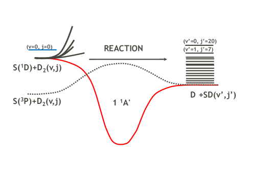
Figure 1: Potential energy surface sketch. At the total energy corresponding to the $D_{2}(v=0,j=0)$ initial state, the $v^{\prime}$=0 and $v^{\prime}$=1 manifolds comprise 20 and 6 rotational states, respectively.

Five singlet PES’s correlate with the reactants asymptote in the title reaction, S(${}^{1}D$)+D₂. However, only two of them, 1${}^{1}A^{\prime}$ and 1${}^{1}A^{\prime\prime}$ correlate adiabatically with the ground state products, SD(${}^{2}\Pi$)+D. The 1${}^{1}A^{\prime\prime}$ surface, which corresponds to a direct abstraction process, has a barrier of 0.43 eV and can be disregarded at low collision energy. The ground state surface, the 1${}^{1}A^{\prime}$, features a deep well in the reaction path ($\approx$4 eV depth), and a relatively small exoergicity ($\Delta_{r}H_{0}^{o}=-0.254$ eV). On this PES, the reaction takes place by insertion of the sulphur atom through the D-D bond, leading to a long-lived intermediate collision complex. Although it has been suggested that the S(${}^{1}D$) $\rightarrow$ S(${}^{3}P$) quenching may play a significant role, quantum scattering calculations considering only the $1A^{\prime}$ PES can reproduce experimental data even at low energies, [48, 55, 49] and this will be our approach here. In Fig. 1, we show a sketch of the different PES’s which correlate with the considered state of the reactants. Apart from the deep well which characterizes the 1$A^{\prime}$ PES, let us note that there are many product rovibrational states which are open at the energies explored in this work. In particular, at the total energies corresponding to the cold and ultracold processes ($E_{c}\leq 1$ K) there are 20 rotational states with $v^{\prime}$=0 and 6 rotational states with $v^{\prime}$=1 accessible from the complex.

In this and our previous works on this system at low kinetic energies, we have used accurate LR interactions [48], and merged them with the short-range interactions provided by the widely used ab initio RKHS PES by Ho et al. [58]. The main terms which characterize the LR interactions are the quadrupole-quadrupole electrostatic term, varying as $\sim R^{-5}$, and the dipole-induced dipole-induced dispersion one, $\sim R^{-6}$. Indeed, the LR potential matrix elements, expressed in a diabatic basis of five asymptotically degenerate atomic states, $|L\lambda\rangle$, corresponding to the 5 values of the $\lambda$ projection of the sulphur orbital angular momentum, $L$=2, on the body-fixed $z$-axis, can be written as: [53]

$$V_{\lambda,\lambda^{\prime}}(R,\theta)= \frac{1}{R^{5}}C_{5}^{\lambda,\lambda^{\prime}}\;{\cal C}_{2,\lambda^{\prime}-\lambda}(\gamma,0)$$

$$-\frac{1}{R^{6}}\sum_{k=0,2}C_{6,k}^{\lambda,\lambda^{\prime}}\;{\cal C}_{k,\lambda^{\prime}-\lambda}(\gamma,0)$$ (1)

where $\gamma$ is the Jacobi angle, the angular functions ${\cal C}_{l,m}(\theta,\phi)$ are the modified spherical harmonics, and the coefficients $C_{5}^{\lambda\lambda^{\prime}}$ and $C_{6,k}^{\lambda\lambda^{\prime}}$ correspond to the electrostatic (quadrupole-quadrupole) and dispersion (dipole-induced dipole-induced) contributions, respectively.

As already mentioned, our treatment of the dynamics for the collision with D₂($j=0$) will be adiabatic. However, if we considered a non-adiabatic treatment using 5 electro-nuclear basis functions (each of them corresponding to an atomic $|L\lambda\rangle$ state), which depend on the coordinates of both atoms and electrons, the contribution of quadrupole-quadrupole and dispersion anisotropic terms would be zero since the potential coupling elements of the type $\langle j=0|P_{2}(\cos\gamma)|j=0\rangle$ vanish. Accordingly, in order to introduce a right dependence of the LR interaction with distance, we have matched the PES by Ho, with a pure isotropic dispersion term of the type $-C_{6}/R^{6}$ around a distance of $R$=13.5 a₀. The value of $C_{6,k=0}^{0,0}$, the lowest isotropic one, was chosen to that purpose, $C_{6}$=41.78 a.u.

II.2 The effective potentials

As explained in Ref. 48 and 46, a convenient basis in order to expand the nuclear wavefunction in the LR region can be characterized by quantum numbers $(J,M,v,j,l)$, with ($J,M$) the total angular momentum and its projection on the Space-Fixed (SF) $Z$ axis, ($v,j$) the rovibrational quantum numbers of the diatom and $l$ the relative orbital angular momentum. We represent it as $\varphi^{JM}_{vjl}$. Now, the matrix element of the electronic potential evaluated for the incoming channel $(J,M,v_{0},j_{0},l_{0})$, plus the centrifugal potential term, can be understood at each distance $R$ as the effective 1D-potential, $V_{\rm eff}(R)$, felt by the colliding partners while approaching:

$$V_{\rm eff}(R)=\langle\varphi^{JM}_{v_{0}j_{0}l_{0}}|V(R,r,\gamma)|\varphi^{JM}_{v_{0}j_{0}l_{0}}\rangle+\frac{l_{0}(l_{0}+1)\hbar^{2}}{2\mu R^{2}}$$ (2)

where $\langle...\rangle$ indicates here the integration over the Jacobi coordinates $r$ and $\gamma$ and $\mu$ is the reduced mass. The evaluation of the potential matrix element, in brief $V_{l_{0},l_{0}}(R)$, involves the change to the helicity basis (labeled by the projection $\Omega_{j}$ of ${\bm{J}}$ on the Body–Fixed (BF) coordinate system, instead of $l$) using $3j$ symbols and leads to the following expression:

$$V_{l_{0},l_{0}}(R)= 2\pi(2l_{0}+1)\,\sum_{\Omega_{j}}{\left(\begin{array}[]{ccc}j_{0}&l_{0}&J\\ \Omega_{j}&0&-\Omega_{j}\end{array}\right)}^{2}$$ (5)

$$\int\chi_{v_{0},j_{0}}^{2}(r)Y_{j_{0}\Omega_{j}}^{2}(\gamma,0)V(R,r,\gamma)\;dr\;d(\cos\gamma).$$

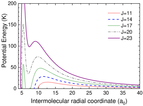
Figure 2: Effective potentials (centrifugal plus electronic potential) for different values of the orbital (here also total) angular momentum. Note the double-maximum structure.

Effective potential for several $J^{\prime}s$ are shown in Fig. 2. They exhibit a double-maximum structure, which was already noted in previous works on the system for other isotopic variants. [59, 55] While the outer maximum is the well known centrifugal barrier, resulting from the increasing attraction to the internal region of the PES and the repulsion of the centrifugal term, the inner maximum has a dynamical character. The latter is due to the angular averaging in $\gamma$ angle (at each $R$), the potential energy being increasingly negative closer to perpendicular angles (insertion) and positive (with a potential barrier appearing) for linear approach.[60] Let us remark that the double maximum structure also appears in the effective potentials calculated using more recent PESs. [55] We have related this structure to the appearance of shape resonances for high partial waves, which would be supported by the potential well between both maxima. [59] The change of slope observed on previously published experimental and theoretical excitation functions can be also attributed to this double maximum structure.[55, 49]

II.3 Dynamical methodology and calculation details

The method based on hyperspherical coordinates developed by Launay et al. [47] has been widely used for thermal and hyperthermal reactive scattering [61, 62, 63, 64]. It uses Smith-Witten hyperspherical democratic coordinates to describe the interaction region of the configuration space and considers a single adiabatic PES. The hyper-radius coordinate, $\rho$, is split into a multitude of sectors, and a coupled channel method of the type diabatic-by-sector is used. The chosen basis of surface functions (which depend on the hyperangles and are defined at the centre of each sector) is particularly appropriate to study insertion reactions with very deep wells. The log-derivative matrix built by expanding the total wavefunction using the sector basis, is propagated outwards in $\rho$, and changed of basis at the border of each sector. Its value at a long enough value of hyper-radius, $\rho_{0}$, is matched to a set of suitable radial functions, called asymptotic functions (AFs). At thermal energies, the AF s are the familiar regular and irregular radial Bessel functions (accounting for the presence of the centrifugal potential). To study cold and ultracold collisions, the AF’s were modified to account for both the centrifugal potential and the particular LR potential existing at $\rho_{0}$ [48, 64, 65, 66]: in this way the AF’s are adapted to each specific LR behavior, ensuring the collisional boundary conditions while working at finite distance. This avoids propagations in hyperspherical coordinates up to extremely large intermolecular separations. We use the coupled-equation version of the method of De Vogelaere [67] to calculate the AF’s in Jacobi coordinates [48] by solving a system of very few differential equations (only one for the case $j$=0). Although propagations from very large radial distances, (where LR interactions are negligible) up to $\rho_{0}$ are required for their calculation, the expense is minimal in comparison with the alternative of propagating directly in hyperspherical coordinates. This implementation is applied here to deal with a system with $\sim R^{-6}$ LR behavior. Let us note that to converge the elastic cross sections at a collision energy of $10^{-8}$ K, De Vogelaere’s propagations starting from separations of $\sim$10⁴ a₀ were needed to calculate the AF’s. However, the computational cost of this calculation is affordable. Reaching so large intermolecular separations using the unmodified (direct) implementation in hyperspherical coordinates would be unthinkable. The AF’s allow to ’bring’ the asymptote to reduced finite distances.

We have calculated quantum reactive cross-sections for the collision S(${}^{1}D$)+ D₂($v$=0, $j$=0)$\rightarrow$ SD + D in the collision energy range 10^-8 K–220 K. This range covers part of the thermal or Langevin regime, where an appreciable number of partial waves are open and the classical Langevin capture model might work (usually 4-5 partial waves are enough), and the cold ($E<$1 K $\sim$ 0.7 cm^-1) and ultracold ($T<$1 mK) regimes. At the energies considered in this work, the Langevin regime can be taken to be comprise the 2 K-220 K range, with 5 and 27 partial waves open, respectively. This can be concluded by examining the height of the effective potentials. Partial waves $J=$0-27 were needed in order to converge the reactive cross sections. The elastic counterparts require higher total angular momenta and they are only converged in partial waves up to approximately 1 K. The number of adiabatic channels in hyperspherical coordinates included in the calculations lies in the range from 380 ($J$=0) to 6605 ($J$=27). The propagation in hyperspherical coordinates was taken from $\rho$=1.8 a₀ up to $\rho_{0}$=16.6 a₀, where the matching to the AFs was performed. The integration to calculate the AF corresponding to the incoming channel at each considered energy was taken from a radial distance where the absolute value of the potential is $10^{-8}\times E$ up to $\rho_{0}$. This amounts to starting at $\approx 10^{4}$ a₀ for the lowest energy considered. Such a stringent criterion was necessary in order to obtain the correct Wigner behavior of the elastic cross sections.

Our calculations yield the $S$-matrix as a function of the energy for each value of $J$ or equivalently $l$, the relative orbital angular momentum (note that in our case $j$=0). The complex (energy dependent) scattering length, $\tilde{a}_{l}(k)=\alpha_{l}(k)-i\beta_{l}(k)$, essential ingredient when considering the ultracold regime, can be evaluated using the elastic elements of the $S$-matrix [68] by applying the expression:

$$\tilde{a}_{lm}(k)=\frac{1}{ik}\,\frac{1-S_{lm,lm}(k)}{1+S_{lm,lm}(k)}$$ (6)

where $k$ is the wavenumber. At low enough collision energy, the complex scattering length relates to the elastic, $\sigma_{\rm el}$, and total-loss cross-section, $\sigma_{\rm loss}$ (which means inelastic $\sigma_{\rm in}$ plus reactive $\sigma_{\rm r}$) in the following way:

$$\sigma^{lm}_{\rm el} \to 4\pi(\alpha_{lm}^{2}+\beta_{lm}^{2})$$ (7)

$$\sigma^{lm}_{\rm loss} \to \frac{4\pi\beta_{lm}}{k}$$ (8)

As long as one is not interested in product-state resolved magnitudes, it must be stressed that all the significant information is contained in the diagonal elements $S_{lm,lm}(k)$ of the S-matrix:

$$\sigma_{\rm el} = \sum_{l,m}\sigma^{lm}_{\rm el}=\frac{\pi}{k^{2}}\sum_{l,m}|1-S_{lm,lm}(k)|^{2}$$ (9)

$$\sigma_{\rm r} = \sum_{l,m}\sigma^{lm}_{\rm r}=\frac{\pi}{k^{2}}\sum_{l,m}[1-|S_{lm,lm}(k)|^{2}]$$ (10)

II.4 Classical Langevin Model

The classical (Langevin) capture model for an $R^{-6}$ potential is used to rationalize the cross sections and rate constants for atom + molecule collisions at thermal energies. This model is approximately valid for collisions dominated by attractive potentials and large reaction probabilities, usually providing an upper-limit to the reaction probability. The assumption is that the reaction occurs whenever the reactants are able to reach the inner part of the PES and interact strongly, that is, whenever the kinetic energy overcomes the centrifugal barrier, and the reactants can get close enough. Besides, it assumes a classical non-quantized orbital angular momentum.

The Langevin expressions for the reaction cross section, $\sigma_{\rm L}(E)$, and rate coefficient, $k_{\rm L}(E)$, can be obtained starting from the quantum expression

$$\sigma_{\rm r}(E)=\sum_{l=0}^{\infty}\sigma^{l}_{\rm r}(E)=(\pi/k^{2})\sum_{l=0}^{\infty}(2l+1)P_{\rm r}^{l}(E),$$ (11)

where $P_{r}^{l}(E)$ is the reaction probability for a particular partial wave $l$ and $m$ projection (we will use $P_{r}^{l}(E)$ or $P_{r}^{J}(E)$ indistinctly in the notation below ($j=0$). By: (i) calculating the centrifugal barrier height for each $l$ corresponding to an analytical potential $-C_{6}/R^{6}$; (ii) assuming that $P_{r}^{l}(E)=1$ if the kinetic energy is higher than the centrifugal barrier, and null otherwise; and (iii) replacing the summation with an integral over continuous values of $l$ (valid for high enough maximum $l$) we obtain the Langevin cross section,

$$\sigma_{\rm L}(E)=3\pi(C_{6}/4E)^{1/3},$$ (12)

and, multiplying by the relative velocity, the Langevin rate coefficient

$$k_{\rm L}(E)=3\pi(C_{6}^{2}E/2\mu^{3})^{1/6}.$$ (13)

These expressions can only be valid when many partial waves are open. In fact, in the limit of vanishing kinetic energy (only $l=0$ is involved) the right Wigner behavior, $\sigma_{\rm r}(E)\sim E^{-1/2}$, is not recovered.

The accuracy of the Langevin model can be improved in reactions mediated by a complex by: (i) calculating the heights of the centrifugal barriers, using the effective potentials, thus accounting for deviations from the $R^{-6}$ behavior at short-range; (ii) carrying out the summation over discrete partial waves instead of an integral over a continuous variable; and (iii) correcting the assumption $P_{\rm r}^{l}(E)=1$ with a statistical factor, $P_{{\rm complex}\to{\rm prod}}$, that is calculated as the ratio between the number of product states and the total number of states (reagents and products), and accounts for the fact that the probability of a complex to decompose into the products arrangement channel will be usually lower than 1. We named this improved model Numerical-Capture Statistical (NCS) model in previous works [46].

In contrast to the D⁺+ H₂ reaction, where $P_{{\rm complex}\to{\rm prod}}$ was significantly lower than 1 [45], there are many SD channels accessible from the well for the S+D₂ reaction (see Fig. 1), and hence the probability flux is expected to be irreversibly lost from the incoming channel due to the numerous couplings inside the well which lead to the product channels.[46, 48] Consequently, most of the complexes will decompose to form the products and very few to give back the reactants. In other words, the NCS model assumes $P_{r}^{J}(E)=1$ in this system, as the Langevin model does, and both models should only differ in the discrete distribution of impact parameters considered by the former.

As the Langevin model, the NCS model does not provide the right behavior in the limit of vanishing kinetic energy. When only s-wave contributes at low enough kinetic energy, and assuming that $P_{\rm r}^{l=0}(E)=1$, we get:

$$\sigma_{\rm r}^{l=0}(E)=\frac{\pi}{k^{2}}P_{\rm r}^{l=0}(E)=\frac{\pi}{k^{2}}\propto E^{-1}$$ (14)

The wrong power stems from the assumption $P_{\rm r}^{l=0}(E)=1$, which clearly does not fulfill the limiting behavior of the reaction probability, that should be $P_{\rm r}^{l=0}(E)\propto E^{1/2}$ as $E\to 0$. Due to the LR forces the incoming flux is reflected back before reaching the SR region of the PES even in the absence of centrifugal barrier, and hence the reaction probability goes to zero. It must be, however, stated that the Langevin’s assumption: “all the flux that reaches the transition state leads to reaction” is not wrong. What is wrong is the mathematical implementation of this assumption in the classical model: $P_{\rm r}^{l=0}(E)=1$ at any energy. There exist other ways to implement Langevin’s idea without violating the Wigner threshold laws using the MQDT.

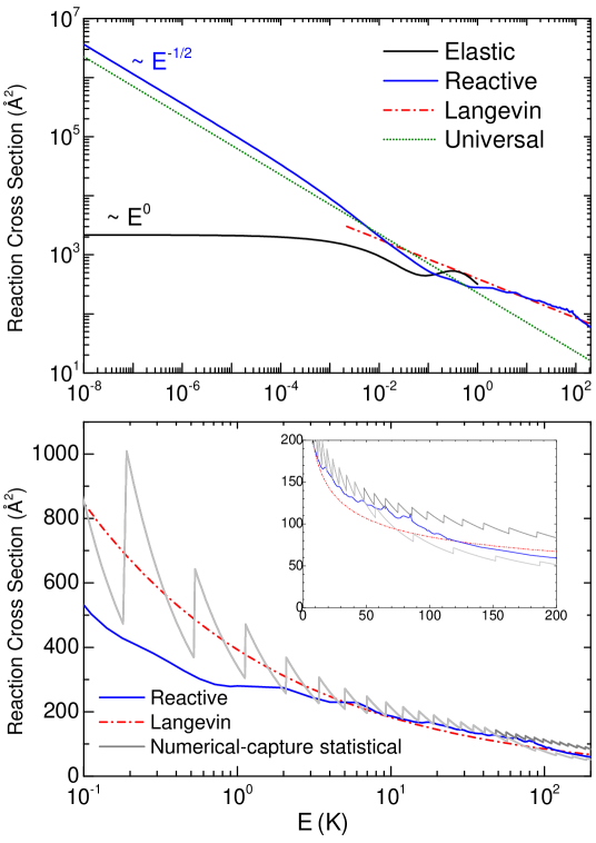
Figure 3: The upper panel displays in logarithmic scale the QM total reaction and elastic cross-sections, whose Wigner limits are $E^{-1/2}$ and $E^{0}$, respectively. The reaction cross-section is compared with the universal prediction at ultra-low collision energies and with the Langevin prediction (with the right $C_{6}$), when many partial waves are open. The lower panel shows the reaction cross sections at the Langevin-regime collision energies. The QM cross sections are compared with the ones obtained using the classical Langevin formula, Eq. (12), and the more realistic numerical-capture statistical model. The inset highlights these latter results in a linear scale of energies.

II.5 Calculating capture probabilities

Under the influence of a particular potential, i.e. $V_{\rm LR}(R)=-C_{6}/R^{-6}$, within a region where the WKB aproximation is valid, one can distinguish between incoming and outgoing probability terms in the continuum wavefunction:

$$\psi(R)\sim\frac{A\exp[-i\int_{R}k(x)dx]+B\exp[+i\int_{R}k(x)dx]}{\sqrt{k(R)}}\,,$$ (15)

where $k(R)=[2\mu(E-V_{\rm LR}(R)]/\hbar$ is the wavenumber at a distance $R$ and $E$ is the collision energy. The formula implies that part of the incident flux is reflected by the potential and part of it is transmitted. However, one can mathematically impose the absence of reflected term (semi-classical condition for perfect absorption or transparency) at a particular point in space, $R_{m}$: the logarithmic derivative of the wavefunction should take there the simple form $Z(R_{m})=-ik$. We say that the flux is captured by the potential and we know this probability as capture probability. In order to determine it, we need to find the solution of the 1D time-independent Schrödinger equation (TISE), with potential $V_{\rm LR}(R)=-C_{6}/R^{-6}$, which fulfills the condition $Z(R)=-ik$ at a short matching distance. Once obtained, the S-matrix element associated to this solution will not have modulus 1, due to the loss of flux at short distances. The lack of unitarity, $1-|S|^{2}$, will be precisely the capture probability we want to calculate. In this work we use the method by De Vogelaere [67] to solve the TISE. More details about the procedure are given in the Appendix.

III Results and Discussion

III.1 The reaction in the Langevin regime

The QM reaction cross section calculated in the low energy region is shown in the bottom panel of Fig. 3 along with the Langevin and NCS results. Interestingly, the Langevin model does not always overestimate the QM result in the range 2-200 K, where enough partial waves are open for the integral to be a good aproximation to the discrete summation in partial waves. Moreover, the slope of the Langevin model, which reveals the pace of the opening of partial waves corresponding to a $R^{-6}$ potential, is not in agreement with the slope of the QM cross section below 120 K (see inset of Fig. 3). Indeed, the $C_{6}/R^{6}$ potential used in the Langevin model is not valid at short radial distances where the centrifugal barriers for moderate $J$ values are located.

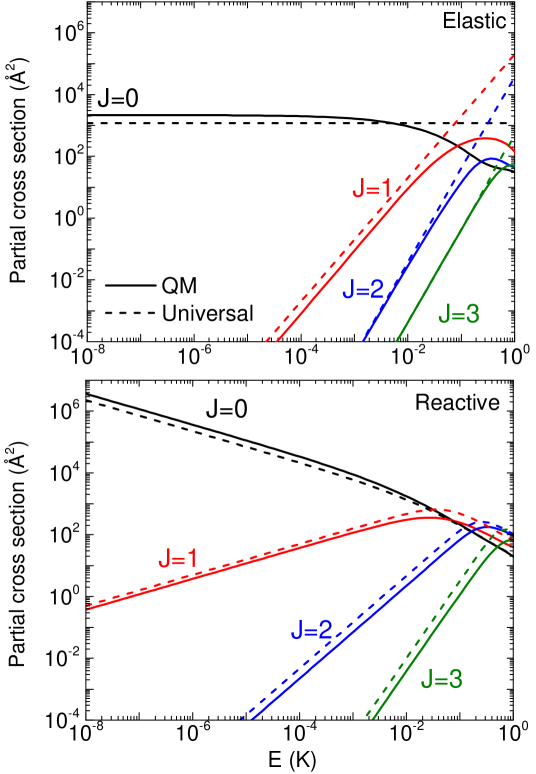
Figure 4: Elastic (upper panel) and reaction (lower panel) cross-sections corresponding to the lowest partial waves for S(${}^{1}D$)+ D₂ ($v$=0, $j$=0) collisions in the cold and ultracold regimes. The QM results are compared with the results of the universal predictions (dashed line).

The NCS model corrects the Langevin model by using the right effective potentials given by Eq. (5) and depicted in Fig. 2. Accordingly, it should provide both an upper limit and the right dependence of the cross-section with the collision energy. Due to the double maximum structure of the effective potentials, special care should be taken when implementing the NCS model; strictly speaking, the highest maximum should be chosen as the one limiting the access of the probability flux to the interaction region. While the outer maximum is higher for lower partial waves, $J<$ 17, it is the inner (dynamical) barrier the one which allegedly limits the reactivity for $J\geq$ 17. The result of this implementation is shown in solid grey line in Fig. 3. The agreement with the QM results is much better than the one obtained using the Langevin expression, both working as a higher bound and following the slope of the QM results up to energies $\sim 50$K (precisely the height of the two barriers associated to $J$=17). At these energies, right where the inner maximum plays a role, the NCS model shows a significant decrease and a sudden change of the average slope, a behavior which is observed in the QM results above $E\approx 90$K. It seems that the effect of the inner maximum is not reflected yet in the QM results for the partial waves in this energy region. To understand this effect, we calculated the NCS model cross sections by considering only the height of the outer maxima, irrespective of whether it is the highest of the two. The results obtained are shown using green colour line in the lower panel of Fig. 3, and are better appreciated in the inset. This second NCS implementation is closer to the QM results up to energies around 90 K, although it is unable to follow the change observed in the QM results at higher energies. Interestingly, the QM value seems to lie between the results of both implementations of the model. This is not difficult to understand in view of the effective potentials: even if the inner barrier is higher than the outer one for $J\geq$ 17, it is very narrow and the tunneling through it is probably very significant. In this scenario, the flux seems to be effectively limited by the outer maximum up to $J\geq$ 21. For higher $J$’s, neither the outer nor the inner barrier heights seem able to characterize the opening of partial waves: the effect of the inner barrier is too significant to be ignored, but the tunneling is also too high to imply that the opening of a partial wave occurs necessarily above it. It is the interplay of both barriers which leads the process.

III.2 Low partial waves in the (ultra)cold regime

To analyze the behavior in the (ultra)cold regime for a LR potential of the form $-C_{n}/R^{n}$ $(n>3)$, it is useful to define a characteristic length, $R_{n}=(2\mu C_{n}/\hbar^{2})^{1/(n-2)}$, and a characteristic energy, $E_{n}=\hbar^{2}/(2\mu R_{n}^{2})$. For the case $n$=6 we get $R_{6}=(2\mu C_{6}/\hbar^{2})^{1/4}$ and $E_{6}=\hbar^{2}/(2\mu R_{6}^{2})$, which amount to $R_{6}=27.2\,a_{0}$ and $E_{6}/k_{B}T\approx 3.3\times 10^{-2}$ K, respectively, when evaluated for the title system . The so-called mean scattering length $\bar{a}$ [57], useful to rationalize the problem, is given in this case by

$$\bar{a}=\frac{2\pi}{\Gamma(1/4)^{2}}R_{6}\approx 13\,a_{0}\,.$$ (16)

In the wilderness of the ultracold regime, the well known Wigner threshold laws [42, 71] work as a compass. They state that the elastic, $\sigma_{\rm el}^{l}$, and the total-loss (inelastic plus reactive) cross section, $\sigma_{\rm loss}^{l}$, associated to each partial wave vary, close to threshold, as:

$$\sigma_{\rm el}^{l} \sim E^{2l}$$ (17)

$$\sigma_{\rm loss}^{l} \sim E^{l-1/2}$$ (18)

Given that H₂($v$=0, $j$=0) is the only rovibrational state of the reactants open at the considered energies, the inelastic process is absent and losses are only associated to reaction, $\sigma_{\rm loss}^{l}=\sigma_{\rm r}^{l}$. Besides, the threshold laws for elastic scattering are modified for a potential with $n=6$. The phase shift for $l>1$ at very low collision energies is dominated by a term $\sim E^{2}$ originating from the dispersion potential.  [42] The anomalous behavior of the elastic cross section is given by

$$\sigma_{\rm el}^{0} \sim E^{2l}~{}~{}\text{for}~{}l=0,1$$ (19)

$$\sigma_{\rm el}^{l} \sim E^{3}~{}~{}\text{for}~{}l>1$$ (20)

In summary, while the partial reaction cross sections are expected to change as $E^{l-1/2}$, the partial elastic ones will remain constant for $l=0$, change linearly with energy for $l=1$ and behave as $E^{3}$ for $l>1$.

These predicted behaviors can be distinguished in Fig. 4, where the reactive (lower panel) and elastic cross sections (upper panel) for the lowest four partial waves, are shown in solid line and log scale. Note the change of slope of the $p$-wave ($J$=$l$=1) reaction cross section at energies around $E_{6}$ (33mK), close to the height of the centrifugal barrier. It is also remarkable the anomalous behavior for $\sigma_{\rm el}^{l}$, with the slope of the elastic cross sections being the same for $l=2,3$. A lack of all the previous limit behaviors in the numerical results would have been taken as an indication that a particular PES is not reliable to describe low energy collisions or that the calculations are not well converged.

The s-wave contribution will dominate in the limit of extremely low kinetic energies, where only $l=0$ is open. The total (vs. partial) reaction cross section should change as $E^{-1/2}$ (the reaction rate coefficient being thus constant) and the total elastic cross section remain constant (the elastic rate coefficient changing as $E^{1/2}$). Note these behaviors in the upper panel of Fig. 3, where total reactive and elastic cross sections are shown. The Langevin prediction is also shown for comparison. Below the range of energies where the number of open partial waves is noticeable, it largely separates from the numerical results and it does not reach the right slope in the ultracold regime . Interestingly enough, this divergence does not necessarily mean that the Langevin assumption (the reaction occurs with almost unit probability when the reactants get close enough) is wrong, but that the probability that the reactants get close enough to react is very low. We will analyze this in the following section.

III.3 The Quantum Langevin behavior

We will consider the quantal version of the Langevin model proposed in the context of MQDT in Ref.  36 (see Appendix for details). The model, that complies with the Wigner laws, allows us to move smoothly from high energies to the ultracold regime under the same assumption: all the flux reaching the SR region leads to reaction. This Langevin-type assumption, translated into the language of the model, is expressed as: the loss probability at SR, $P^{\rm re}$, is one, which is known as the universal behavior. Let us recall that $P^{\rm re}$, which is related to the $y$ parameter (see Appendix), denotes the flux that is irreversibly lost from the incoming channel at SR, and is not directly observable nor necessarily coincides with the reaction probability, $P_{r}^{J}(E)$. Expressed in simple terms, the incoming flux which leads to reaction has to overcome two obstacles: (i) it needs to reach the SR or transition state region without being reflected backwards by the LR or centrifugal potential; (ii) it has to find its way from the SR region to the products valley; this latter process is the one accounted for by the $P^{\rm re}$ parameter. We can conclude that only at high energies, when quantum reflection by the LR potential and tunneling through the centrifugal barrier are negligible, $P_{r}^{J}(E)\approx P^{\rm re}$. Furthermore, the expression

$$\sigma_{\rm r}(E)\approx P^{\rm re}\cdot\sigma_{\rm L}(E)$$ (21)

would be valid in the Langevin regime if $P^{\rm re}$ were weakly dependent on the energy and the partial wave [36]. According to Fig. 3, the title reaction fulfills Eq. 21 in the limited range 5 K-15 K with $P^{\rm re}=1$. However, the deviation of $\sigma_{\rm L}(E)$ from $\sigma_{\rm r}(E)$ at higher energies was not due to the failure of the Langevin’s hypothesis, but to the inability of a pure $R^{-6}$ term to account for the heights of the centrifugal barriers (which occur at short distances) for higher $J$’s. In essence, it would be more precise to substitute $\sigma_{\rm NCS}$ (with statistical factor 1) for $\sigma_{\rm L}$ in equation Eq.(21), hence finding that $P^{\rm re}$ is closer to 1 in a much wider range. Besides, in a previous work we established a link between $P^{\rm re}$ and the statistical factor $P_{{\rm complex}\to{\rm prod}}$, and hence a way to estimate the parameter $y$. [45] As indicated above, we can assume that $P_{{\rm complex}\to{\rm prod}}\approx 1$ in the title system, leading again to $P^{\rm re}\approx 1$ and $y\approx 1$. In conclusion: we can consider the system as roughly universal or quantum-Langevin.

It would be interesting to compare the QM results with the behavior of a universal system. Let us focus first in the reaction cross-sections, which in the case $y=1$ are given by the capture probabilities. Using De Vogelare’s method and proceeding as described in the Appendix, we have calculated the capture probabilities, as a function of the energy, corresponding to a pure $-C_{6}/R^{6}$ potential for the lowest partial waves; using them we have obtained the partial cross-sections. They are shown in dashed line in the lower panel of Fig.4, where they are compared with the QM ones. The behavior for $J$=0 and $J$=1 in the ultracold limit is given by Eq. (33) and Eq. (35), stemming from Ref. 37. The limiting ratios of the QM and capture values of the cross-sections as $E\to 0$ are 1.6, 0.7, 0.5, 0.4 and 0.8 for $J$=0, 1, 2, 3 and 4 respectively. Note that for $J>0$ the cross-sections show a maximum as a function of the energy which is related to the height of the centrifugal barrier. As only for low partial waves the centrifugal barrier is well reproduced by a pure $-C_{6}/R^{6}$ asymptotic potential, the maxima in the QM and the capture calculations show increasing differences as $J$ grows.

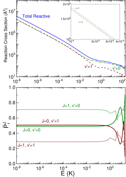
Figure 5: Upper panel: Total reaction cross section as a function of the collision energy (blue solid line) together with the vibrationally resolved cross sections ($v^{\prime}$=0 green and $v^{\prime}$=1 brown dash-dotted lines). For $E<10^{-2}$ K the cross section into $v^{\prime}$=1 is larger than that into $v^{\prime}$=0 (see inset). Lower panel: fraction of collisions at a given $J$ leading to $v^{\prime}$=1 (brown line) and to $v^{\prime}$=0 (green line) for total angular momentum $J$=0 (solid line) and $J$=1 (dashed line). At $E>5\cdot 10^{-1}$ K the fraction into $v^{\prime}$=0 takes over and even for $J$=0 no vibrational population inversion is found. Note that the contribution of $J$=1 is negligible for $E<10^{-3}$ K (see fig.4).

Regarding the elastic cross-sections, Ref. 37 only provides their limit behavior for $J$=0 and $J$=1, Eq. (34) and Eq. (36). It is possible to generalize these expressions and calculate the partial cross sections for any partial wave with anomalous behavior using Eq. (7): $\alpha_{lm}$ can be obtained using the Born-approximation (see Eq. (44) the Appendix); $\beta_{lm}$ is directly related to the numerical capture probabilities we have calculated using Eq. (8). The universal partial elastic cross-sections are shown in dashed line in the upper panel of Fig.4, where they are compared with the QM ones. The limit ratios of the QM results and the universal values are 1.8, 0.4, 0.9, 1 and 1 for $J$=0, 1, 2, 3 and 4 respectively.

The agreement between the QM results and the universal ones is on the same order of magnitude of the one we obtained in our previous study on the system D⁺+ H₂ when applying the MQDT model. What is remarkable is that the QM reaction cross-section for $J$=0 is higher than the universal prediction, which implies that the reaction probability is higher than the total capture. One of the interesting predictions of the MQDT model is precisely that the reaction probability at ultracold energies is not limited by the capture or probability transmitted by the LR potential. In fact, by recalling that the reaction probability can be related to the imaginary part of the scattering length, $P_{r}^{l}(E)=4k\beta_{l}$, and using Eq. (27), we get the following limit behavior for $l=0$ in the general, non-necessarily universal, case:

$$P_{r}^{l=0}(E)=4k\,\beta_{0}(k)=4k\bar{a}\times y\,\frac{1+(1-s)^{2}}{1+y^{2}(1-s)^{2}}$$ (22)

The first factor, $4k\bar{a}$, is the limit value of the capture probability ($P_{r}^{l=0}$ when $y$=1), and the second factor can be higher than 1 for values of $y\neq 1$, and for high enough values of $s$, what can be usually associated to the presence of resonant states close to threshold. We conclude that the reaction probability can be higher than the capture probability, however counterintuitive this idea may appear. This seems to be the behavior in the title system (see the corresponding cross-sections in the upper panel of Fig. 3).

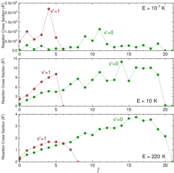
Figure 6: State-to-state integral reaction cross-sections at 10^-7  K (upper panel), 10 K (middle panel) and 220 K (bottom panel) collision energy for $v^{\prime}$=0 (green) and $v^{\prime}$=1.

III.4 The rovibrational state distribution in the ultracold regime

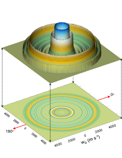
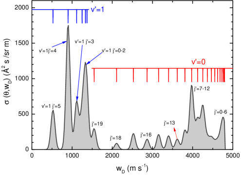
Figure 7: Upper panel: Polar map showing the angular and recoil velocity distribution of the scattered D product in the center-of-mass frame at the collision energy of 10^-7 K. At this collision energy the only significant contribution proceeds from $J$=0; hence the differential cross section is isotropic. Lower panel: D-atom distribution of recoil velocities corresponding to the indicated SD rovibrational states at any angle. As can be seen, the intensity of the peaks correlating with the SD rotational states of $v^{\prime}$=1 prevail over those of $v^{\prime}$=0. The comb shows the center of D-atom recoil that corresponds to the various internal states of the SD co-product. An arbitrary width of 120 m s^-1 has been employed in the Gaussian functions that mimic the D velocities associated to the various SD rovibrational states.

The availability of accurate QM results for the system provides a good opportunity to investigate whether the final state distribution complies with the statistical assumption in the ultracold regime. Specifically, the S(${}^{1}D$)+H₂ reaction and its isotopic variants have been considered as benchmarks of the statistical model assumptions: the transition probability from an initial $i$ state to a final $f$ state is expressed as the product of the capture probability from channel $i$ and the fraction of collision complexes that decay into the product channel $f$; that is,

$$P_{i\to f}=P_{i}^{\rm cap}\cdot P_{{\rm complex}\to f}$$ (23)

The breakdown of the collision complex is essentially ergodic and hence the spacial and state distributions are essentially statistical. Statistical models [44, 52, 51, 50, 73] applied to S(${}^{1}D$)+H₂ have shown that at thermal and hyperthermal energies the overall (coarse-grained) description of the reaction is in very good agreement with accurate QM scattering calculations.[61, 63, 60, 74] However, an important issue to be discerned is whether the statistical characterization of the reaction holds at the cold and especially at the ultracold regimes.

The upper panel of Fig. 5 shows the vibrationally resolved reaction cross-section that includes the contributions from all the $J$ partial waves. As can be seen, the energy dependence of the vibrationally resolved cross sections follows the Wigner law. In addition, quite remarkably, a vibrational population inversion is observed at ultracold energies below $10^{-2}$ K, where $J$=0 prevails (see inset), at variance with the expectations of the statistical model. At higher collision energies, however, the ground vibrational state of SD becomes more populated than $v^{\prime}$=1. To further investigate this effect, the lower panel of Fig. 5 displays the relative fraction of reactive collisions, ${\bar{P}}^{J}_{r}=\sigma(v^{\prime})/\sum_{v^{\prime}}\sigma(v^{\prime})$, leading to $v^{\prime}$=0 and $v^{\prime}$=1 for $J$=0 and $J$=1 as a function of the collision energy. For $J$=1 the relative probability is constant at collision energies below 0.2 K, and $\approx$30% of the collisions appear in $v^{\prime}$=1. In contrast, for $J$=0 the fraction of collisions into $v^{\prime}$=1 is $\approx$52%, being also constant at lower energies. At energies above 0.2 K, ${\bar{P}}^{J=0}_{r}$ for $v^{\prime}$=1 decreases rapidly, and except for some specific energies, the population inversion no longer takes place.

The next step is to investigate the rovibrational distributions, $\sigma_{r}(v^{\prime},j^{\prime};E)$, of the SD product at energies in the ultracold, cold and thermal regimes. Fig. 6 displays the rotational distributions for $v^{\prime}$=0 and $v^{\prime}$=1 at $10^{-7}$ K (upper panel), 10 K (middle panel) and 220 K (bottom panel) collision energies. At $10^{-7}$ K $J$=0 is the only contribution. At 10 K $J_{\max}$ is 11. In both cases, the highest rotational states that can be populated are $j^{\prime}$=19 and $j^{\prime}$=5 for $v^{\prime}$=0 and $v^{\prime}$=1, respectively, since the available energy proceeds from the exoergicity of the reaction. At 220 K $J_{\max}$=25, exceeding the value of the highest accessible $j^{\prime}$ state ($j^{\prime}$=20) for $v^{\prime}$=0. Relevant to these three cases is the general preference for populating $v^{\prime}$=1 when considering the same $j^{\prime}$ value. Indeed, at the three energies shown in Fig. 6, the cross sections for $j^{\prime}\leq 5$ are larger for $v^{\prime}$=1. Moreover, at ultracold energies, this preference is large enough that when summed over rotational states, there is an slight vibrational inversion for $v^{\prime}$=1 products.

The main assumption of the statistical model is that all the states compatible with parity, conservation of energy and angular momentum are equally populated. A somewhat more refined version, includes the surmounting of the effective barrier (including the centrifugal term). An approximate expression of the cross section for the statistical model when the only initial state is $v$=0, $j$=0 (hence even diatomic parity and $(-1)^{J}$ triatomic parity), can be written as:

$$\sigma(v^{\prime},j^{\prime};E)= \frac{\pi}{k^{2}}\sum_{J}(2J+1)\times$$

$$p^{J}_{0,0}\frac{[\min(J,j^{\prime})+1]\Theta[E^{\prime}_{T}-V_{\rm eff}]}{D^{J}}\,,$$ (24)

where $p^{J}_{0,0}$ is the capture from the D₂($v$=0, $j$=0) initial state, $\Theta(E^{\prime}_{T}-V_{\rm eff})$ is the Heaviside function such that if the product’s translational energy, $E^{\prime}_{T}(v^{\prime},j^{\prime})$, is smaller than the effective barrier in the exit channel, whose centrifugal term depends on $l^{\prime}$, no reaction takes place. The denominator $D^{J}$ is the sum of capture probabilities to both the initial state and all the product states:

$$D^{J}=p^{J}_{0,0}+\sum_{{\rm}all\,\,v^{\prime},j^{\prime}}[\min(J,j^{\prime})+1]\Theta[E^{\prime}_{T}-V_{\rm eff}]$$ (25)

The crucial term is $[\min(J,j^{\prime})+1]$, that represents the number of projections, hence the number of helicity states for given values of $J$ and $j^{\prime}$. Note that as the initial rotational state is $j$=0, there is only one parity and the number of helicities, $\Omega^{\prime}$, is $[\min(J,j^{\prime})+1]$ and not $[2\min(J,j^{\prime})+1]$ as in those cases where two triatomic parities are involved. Following Eq. (24), the statistical prediction at $10^{-7}$ K, for which there is only a single projection, $\Omega^{\prime}$=0, is that all rovibrational states would exhibit the same cross section. However, although all rotational states are populated, as shown in Fig. 6, there are significant deviations from this expectation. Even if we leave aside the presence of peaks at $j^{\prime}$=9, 11 for $v^{\prime}$=0, and $j^{\prime}$=4 for $v^{\prime}$=1, whose origin has to be dynamical, the rotational states for $v^{\prime}$=1 are more populated. This is an indication of the preference for those states with the largest content of internal energy. The internal energy of the rotational states of $v^{\prime}$=1 is only comparable to those of highest rotational states of $v^{\prime}$=0 populated ($j^{\prime}$=19, 20) and, as mentioned, they should exhibit similar cross sections. However, when $J$=0, $l^{\prime}=j^{\prime}$ and therefore highly excited rotational states, whose available translational energy is very small, will be subject to the highest centrifugal barriers in the exit channel. Consequently, the rotational states of the $v^{\prime}$=1 manifold display a larger cross section. It is clear that in the ultracold regime, the reaction cross sections are dominated by dynamical features (oscillations, sharp peaks) that stand out against the usual statistical pattern that can be found at higher energies.

Indeed, apart from some conspicuous oscillations (minima and maxima) whose origin is doubtless dynamical, the rotational distributions at 10 K seem to conform better with the statistical behavior that can be found at thermal and hyperthermal energies. At this energy $J_{\max}\approx 11$, giving rise to many more projections, whose number increases with $j^{\prime}$ until $j^{\prime}$=11. For $v^{\prime}$=0, 1 the behavior follows the statistical pattern: the cross section increases with $(j^{\prime}+1)$ until the limiting value energetically allowed. In both cases the slope resulting from plotting the ratio $\sigma(v^{\prime},j^{\prime})/\sigma(v^{\prime},0)$ vs. $(j^{\prime}+1)$ for $j^{\prime}<$11 is close to one.

At 220 K , where many partial waves contribute to all the states, the behavior is essentially statistical. The cross section is proportional to $(j^{\prime}+1)$ up to $j^{\prime}$=15 for $v^{\prime}$=0. The cross sections of $j^{\prime}$ states with $v^{\prime}$=1 become closer to the respective rotational states with $v^{\prime}$=0.

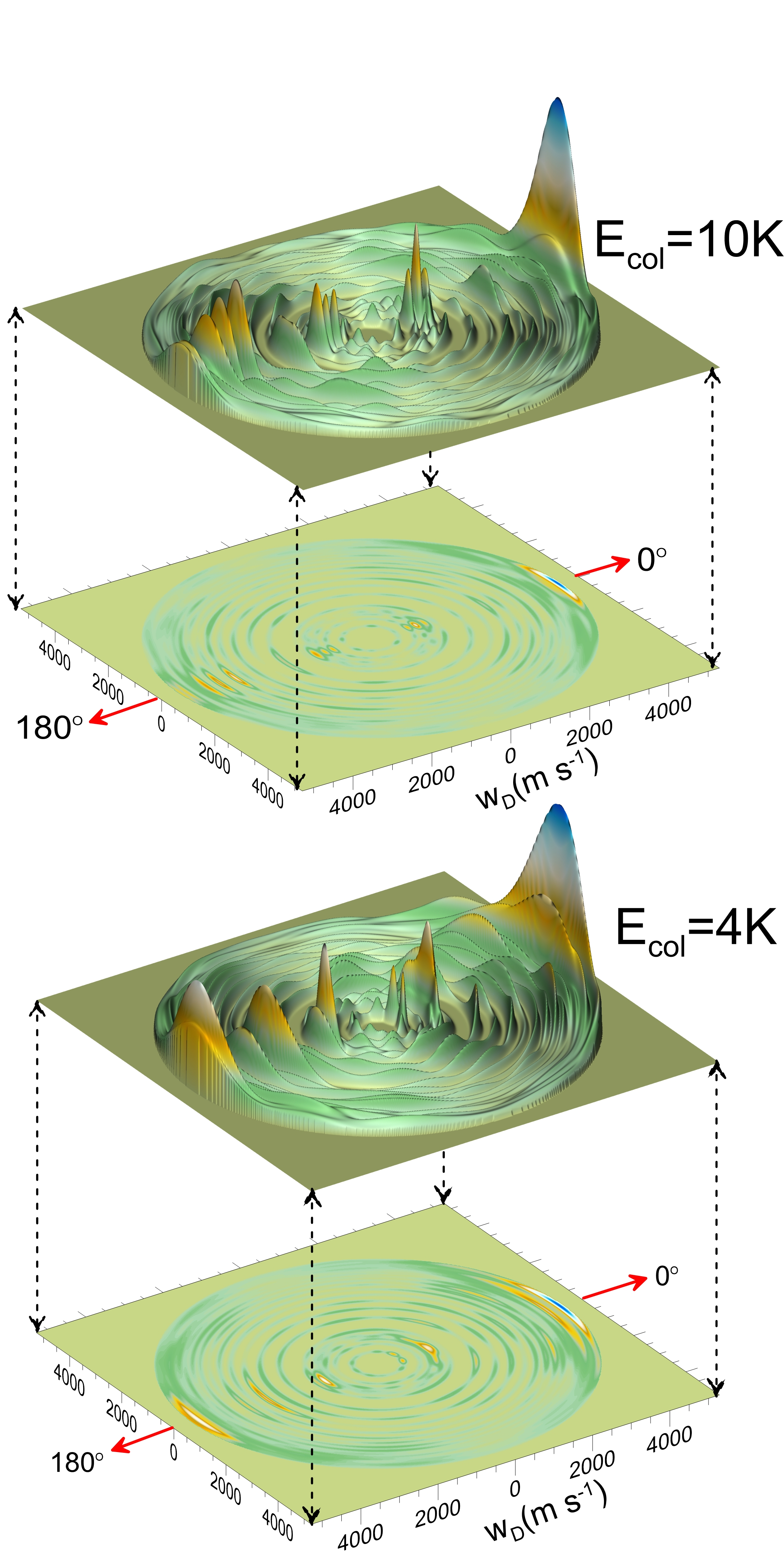
Figure 8: Same as in Fig.7 at the collision energies of 10 K (upper panel) and 4 K (bottom panel). In both cases, there is a predominance for forward scattering. Note that the scattering angle is defined as the angle between the recoil direction of the SD moiety and that of the incoming S atom. The inner rings correspond to the $v^{\prime}$=1 manifold.

The main conclusion of the observed rovibrational distributions is that the dynamical effects prevail over the statistical behavior at collision energies where only few partial waves are open ($<10$ K). In the ultracold regime, when only the s-partial wave comes about, the effect is even more striking since the statistical prediction, apart from the centrifugal barrier in the exit channel, would assign the same weight to all states, $[\min(J=0,j^{\prime})+1]=1$. Of course, the specific features that show up in the calculations are dependent on the PES and subject to its accuracy, therefore should be taken with caution.

The double differential cross sections (DCS), that is, the joint angular and recoil velocity distributions of the D-atom product, are portrayed in Figs. 7 and 8. These polar maps would be similar to those that could be observed experimentally (for instance, using D-atom Rydberg tagging or VMI after ionization of D) if the angle-recoil velocity of the emerging D-atom were observed with a resolution of $\approx$120 m s^-1. The DCS at 10^-7 K, shown in the upper panel of Fig. 7, is isotropic since only $J$=0 contributes to the scattering. The distribution of the D-atom center-of-mass recoil velocity is shown in the lower panel of Fig. 7 and corresponds to the rovibrational distribution shown in Fig 6. As could be expected, the peaks of the $v^{\prime}$=1 rotational states are considerably more pronounced than those from $v^{\prime}$=0.

The polar maps at 10 K and 4 K are shown in Fig. 8. They are no longer isotropic, with some preponderance of forward scattering (the direction of the incoming S(¹D) atom). A strict statistical behavior would have implied a forward-backward symmetry in DCS. However, a lack of symmetry can be also expected within the statistical ansatz, as it has been discussed previously for the S(¹D)+H₂ reaction , and previous calculations have shown that the preference towards forward or backward scattering varies markedly with small changes in the collision energy.[75, 56] Although there is not vibrational population inversion, the sharp peaks associated to rotational states of $v^{\prime}$=1 (inner rings) are conspicuous.

IV Summary and Conclusions

Fully converged, nearly exact adiabatic quantum mechanical calculations have been performed for elastic and reactive S(¹D)+H${}_{2}(v=0,j=0)$ collisions at energies, $E/k_{B}T$, between 10^-8 K and 220 K, covering the ranges of ultracold, cold and thermal regimes.

Since the reaction is barrierless and complex-mediated, the Langevin model is likely to provide a rough estimate of the QM reaction cross section in the thermal and upper-cold regime. In this work, the classical Langevin model has been improved using a numerical capture statistical model that includes discretization of the angular momentum and uses the actual heights of the effective potential in the entrance channel. It is shown, however, that the Langevin model is not applicable in the ultracold regime since it does not fulfil the limiting Wigner threshold behavior.

The universal system, as defined in the Multi-Quantum-Defect theory (MQDT), constitutes a good model for complex-mediated systems where the number of product states is so high that we can assume that most of the probability is irreversibly dissipated from the incoming channel into the well. The agreement between the QM results and the results from the universal model is satisfactory (factors lower than 2 in terms of partial cross-sections) for low partial waves and on the same order of magnitude than those obtained in the study of the D⁺ +H₂ system, where the QM results were compared with those obtained by the MQDT expressions for a non-universal case. Interestingly, it is found that the reaction probability in the ultracold limit is higher than the capture value. The paradox is partially resolved bearing in mind that there is no quantum condition for a perfect quantum absorption, and we are simply finding the solution using an approximate semiclassical boundary condition.

State-to-state integral and differential cross sections are also shown at several collision energies. The QM results indicate that the statistical behavior of the rovibrational distributions is only partially fulfilled below 10 K. In particular, the calculations show that there is a vibrational population inversion in the ultracold regime, where only $J$=0 contributes. Based on statistical grounds, when $J$=0 is the only partial wave ($E<10^{-2}$ K) we can expect that all the rovibrational states are equally populated if the effect of the centrifugal barrier is disregarded. However, under these conditions it seems that dynamical effects outweigh the statistical behavior. By increasing the collision energy, the state resolved integral cross sections follow the expected pattern characteristic of statistical behavior, as demonstrated by the fact that the final-state resolved cross sections are proportional to $(j^{\prime}+1)$. Although the differential cross sections at ultracold energies are necessarily isotropic, the velocity distribution reflects the population inversion of the SD products. As the collision energy increases, the angular distributions are not isotropic any longer, and exhibit the expected forward-backward symmetry characteristic of statistical reactions albeit with some preponderance for forward scattering.

V Appendix

V.1 The Multi-Quantum Defect theory (MQDT) model

The formalism in Ref. [36] provides expressions for the complex (energy dependent) scattering length, $\tilde{a}_{l}(k)=\alpha_{l}(k)-i\beta_{l}(k)$ in terms of the MQDT functions. This allows to parameterize $\tilde{a}_{l}(k)$ using two real parameters, $y$ and $s$, together with the mean scattering length, $\bar{a}$, given by Eq. (16). Specifically, the parameter $0\leq y\leq 1$ characterizes the loss probability at short range, i.e. the flux which is lost from the incoming channel at SR, $P^{\rm re}$, according to $P^{\rm re}=4y/(1+y)^{2}$. The dimensionless scattering length, ${s=\tan\phi}$, is related to an entrance channel phase $\phi$. [36, 37, 76]. In terms of these parameters, and following Ref. 37, the small $k$ behavior of the complex scattering length for the lowest partial waves ($l=0,1$) in the case $n$=6 is given by:

$$\alpha_{0}(k) \to\bar{a}\,\frac{s+y^{2}(1-s)(2-s)}{1+y^{2}(1-s)^{2}},$$ (26)

$$\beta_{0}(k) \to y\,\frac{1+(1-s)^{2}}{1+y^{2}(1-s)^{2}}\,\bar{a},$$ (27)

$$\alpha_{1}(k) \to-2\bar{a}_{1}\,(k\bar{a})^{2}\,\frac{y^{2}s+(s-1)(s-2)}{y^{2}s^{2}+(s-2)^{2}},$$ (28)

$$\beta_{1}(k) \to-2\bar{a}_{1}\,(k\bar{a})^{2}\,\frac{y(2s-s^{2}-2)}{y^{2}s^{2}+(s-2)^{2}},$$ (29)

where

$$\bar{a}_{1}=\bar{a}\,\Gamma(1/4)^{6}/(144\pi^{2}/\Gamma(3/4)^{2})\approx 1.064\,\bar{a}\,.$$ (30)

A quantum Langevin behavior or universal case would correspond to $y=1$. Particularizing expressions  (26)-(28) to this case we get:

$$\alpha_{0}(k) \to\bar{a},\quad\beta_{0}(k)\to\bar{a}$$ (31)

$$\alpha_{1}(k) \to-\bar{a}_{1}\,(k\bar{a})^{2}\,,\qquad\beta_{1}(k)\to\bar{a}_{1}\,(k\bar{a})^{2}$$ (32)

Using Eqs.(7) and (8), we can get the values of the elastic and reaction cross-sections for the two lower partial waves:

$$\sigma^{00}_{\rm r}(E) \to 4\pi\bar{a}\left(\frac{\hbar^{2}}{2\mu E}\right)^{1/2}\,,$$ (33)

$$\sigma^{00}_{\rm el}(E) \to 8\pi{\bar{a}}^{2}\,,$$ (34)

$$\sigma^{1m}_{\rm r}(E) \to 4\pi\bar{a}_{1}{\bar{a}}^{2}\left(\frac{2\mu E}{\hbar^{2}}\right)^{1/2}\,,$$ (35)

$$\sigma^{1m}_{\rm el}(E) \to 8\pi(\bar{a}_{1}{\bar{a}}^{2})^{2}\left(\frac{2\mu E}{\hbar^{2}}\right)^{2}$$ (36)

V.2 Calculating capture probabilities

Following the approach of the MQDT model [36], we can assume that, as the collision partners approach, the incoming probability flux remains associated to the incoming channel, submitted to the $V_{LR}(R)=-C_{6}/R^{-6}$ LR potential. The 1D radial TISE (in reduced form) corresponding to that channel is given by

$$\left[-\frac{\hbar^{2}}{2\mu}\frac{\partial^{2}}{\partial R^{2}}+\frac{l(l+1)\hbar^{2}}{2\mu R^{2}}+V_{LR}(R)\right]\psi(R)=E\psi(R),$$ (37)

Only at short distances, lower that a hypothetical $R_{0}$, the probability is transferred to other collision channels. Assuming the validity of the WKB approximation in an intermediate region ($R_{0}<R<<R_{6}$), we can distinguish incoming and outgoing terms in the solution to the equation, and express it as:

$$\psi(R)\sim\frac{e^{-i\int_{R}k(x)dx}}{\sqrt{k(R)}}-(1-P^{\rm re})^{1/2}e^{i\phi}\frac{e^{+i\int_{R}k(x)dx}}{\sqrt{k(R)}}$$ (38)

where $k(x)=\sqrt{2\mu(E-V_{\rm LR}(x))}/\hbar$. The first term represents the incoming probability flux, and the second one the reflected one. If $P^{\rm re}$ notes the probability which is irreversibly lost from the incoming channel at short range, the reflected probability is $(1-P^{\rm re}).$ Hence we can write the amplitude of the reflected term as $(1-P^{\rm re})^{1/2}e^{i\phi}$, where $\phi$ accounts for any possible phase difference between both. The real and imaginary parts of the logaritmic derivative at a particular point of the considered region, $Z(R)=\psi^{\prime}(R)/\psi(R)$, are given by:

$$Re(Z) = -\frac{k}{2k^{\prime}}$$

$$Im(Z) = -k\left[\frac{P^{\rm re}+2(1-P^{\rm re})^{1/2}\sin\phi}{2-P^{\rm re}-2(1-P^{\rm re})^{1/2}\cos\phi}\right]$$ (39)

The capture probability corresponds to the case $P^{\rm re}=1$, which means a perfect absorption (no reflection term) at SR. The logarithmic derivative takes then a very simplified form $Z(R)=-ik$ (the real part can be neglected if the WKB approximation is fulfilled). We can use the method by De Vogelaere [67] to find a solution with such a logarithmic derivative at a particular matching point $R_{m}$. We proceed as follows. By inwards integration, we obtain the “regular” ($F^{(1)}_{l}$) and “irregular” ($F^{(2)}_{l}$) solutions, defined as the ones which behave as

$$F^{(1)}_{l}(R) \stackrel{{\scriptstyle R>>R_{6}}}{{\longrightarrow}}k^{1/2}R\,\,j_{l}(kR)\stackrel{{\scriptstyle R\to\infty}}{{\longrightarrow}}\frac{\sin(kR-l\pi/2)}{k^{1/2}},$$

$$F^{(2)}_{l}(R) \stackrel{{\scriptstyle R>>R_{6}}}{{\longrightarrow}}k^{1/2}R\,\,n_{l}(kR)\stackrel{{\scriptstyle R\to\infty}}{{\longrightarrow}}-\frac{\cos(kR-l\pi/2)}{k^{1/2}},$$ (40)

where $j_{l}$ and $n_{l}$ are the regular and irregular spherical Bessel functions. As usual, we assume that the asymptotic behavior of the wavefunction is given by ${\psi(r)\sim k^{1/2}R[j_{l}(kR)-\tan(\delta_{l})n_{l}(kR)]}$ at long distance, $\delta_{l}$ being the phase shift, and hence by ${\psi(r)\sim F^{(1)}_{l}-\tan(\delta_{l})F^{(2)}}$ at shorter radius. In particular, at a point $R_{m}$ (where the WKB approximation is fulfilled) we equate $\psi^{\prime}(r)/\psi(r)$ to the perfect absorption logarithmic derivative, $Z(R)=-ik$, and solve for the value of $\tan(\delta_{l})$, also called reactance matrix $K$. We obtain

$$\!\!\!K(E)=\tan\delta_{l}(E)=\frac{F^{(1)}_{l}(R_{m})-Z(R_{m})F^{\prime(1)}_{l}(R_{m})}{F^{(2)}_{l}(R_{m})-Z(R_{m})F^{\prime(2)}_{l}(R_{m})}$$ (41)

And the value of the $S$-matrix is given by

$$S(E)=e^{2i\delta_{l}}=\frac{1+iK(E)}{1-iK(E)}$$ (42)

The obtained S-matrix element will not have modulus 1, due to the loss of flux at short distances. The lack of unitarity, $1-|S|^{2}$ is precisely the capture probability. Let us finally note that partial absorptions and the corresponding S-matrix elements can be simulated by matching to any other value of the logarithmic derivative given by Eq. V.2.

V.3 Calculation of the real part of the $l$-dependent complex scattering length in the case of anomalous behavior

In the case of a LR interaction of the type $V_{\rm LR}(R)=-C_{6}/R^{-6}$, and for values of $l>1$, the phase shift is dominated by a term $\sim E^{2}$. We talk of anomalous behavior. The main contribution to the phase shift is due to the LR part of the potential. It is precisely in this region where the potential is weak enough for the Born approximation to work and we can use it to calculate the phase shift. Following Chapter V, section 2, of Ref. [78], the phase shift as a function of $l$ is given by

$$\delta_{l}=\frac{3\pi\mu C_{6}k^{4}}{16\hbar^{2}(l+5/2)(l+3/2)(l+1/2)(l-1/2)(l-3/2)}$$ (43)

Using this expression, the real part of the scattering length is

$$\alpha_{l}=-\frac{1}{k}\tan\delta_{l}\stackrel{{\scriptstyle E\rightarrow 0}}{{\longrightarrow}}-\frac{3\pi\mu C_{6}k^{3}}{16\hbar^{2}(l+5/2)(l+3/2)(l+1/2)(l-1/2)(l-3/2)}$$ (44)

VI acknowledgments

M. L. is very grateful to J.-M. Launay for his kind help and support, to Andrea Simoni for his insightful discussions and helpful comments, and to K. Jachymski for his willingness to provide details of on his MQDT theory. M. L. and F.J.A. acknowledge funding by the Spanish Ministry of Science and Innovation (Grants No. PGC2018-096444-B-I00 and PID2021-122839NB-I00). P.G.J. acknowledges grant PID2020-113147GA-I00 funded by MCIN/AEI/10.13039/501100011033.

References

- Henson et al. [2012] A. B. Henson, S. Gersten, Y. Shagam, J. Narevicius, and E. Narevicius, Science 338, 234 (2012).
- Shagam and Narevicius [2013] Y. Shagam and E. Narevicius, J. Phys. Chem. C 117, 22454 (2013).
- Narevicius and Raizen [2012] E. Narevicius and M. G. Raizen, Chem. Rev. 112, 4879 (2012).
- Shagam and Narevicius [2012] Y. Shagam and E. Narevicius, Phys. Rev. A 85, 053406 (2012).
- Lavert-Ofir et al. [2014] E. Lavert-Ofir, Y. Shagan, A. B. Henson, S. Gersten, J. Klos, P. Zuchowski, J. Narevicius, and E. Narevicius, Nat. Chem. 6, 332 (2014).
- Osterwalder [2015] A. Osterwalder, EPJ Tech. and Instrum. 2, 10 (2015).
- Gordon et al. [2018] S. D. S. Gordon, J. J. Omiste, J. Zou, S. Tanteri, P. Brumer, and A. Osterwalder, Nat. Chem. 10, 1190 (2018).
- Paliwal et al. [2021] P. Paliwal, N. Deb, D. M. Reich, A. van der Avoird, C. P. Koch, and E. Narevicius, Nat. Chem. 13, 94 (2021).
- Plomp et al. [2021] V. Plomp, X.-D. Wang, F. Lique, J. Klos, J. Onvlee, and S. Y. T. van de Meerakker, J. Phys. Chem. Lett. 12, 12210 (2021).
- Staanum et al. [2006] P. Staanum, S. D. Kraft, J. Lange, R. Wester, and M. Weidemüller, Phys. Rev. Lett. 96, 023201 (2006).
- Zahzam et al. [2006] N. Zahzam, T. Vogt, M. Mudrich, D. Comparat, and P. Pillet, Phys. Rev. Lett. 96, 023202 (2006).
- Wynar et al. [2000] R. Wynar, R. S. Freeland, D. J. Han, C. Ryu, and D. J. Heinzen, Science 287, 1016 (2000).
- Mukaiyama et al. [2004] T. Mukaiyama, J. R. Abo-Shaeer, K. Xu, J. K. Chin, and W. Ketterle, Phys. Rev. Lett. 92, 180402 (2004).
- Syassen et al. [2006] N. Syassen, T. Volz, S. Teichmann, S. Dürr, and G. Rempe, Phys. Rev. A 74, 062706 (2006).
- Hudson et al. [2008] E. R. Hudson, N. B. Gilfoy, S. Kotochigova, J. M. Sage, and D. DeMille, Phys. Rev. Lett. 100, 203201 (2008).
- Ospelkaus et al. [2010] S. Ospelkaus, K.-K. Ni, D. Wang, M. H. G. de Miranda, B. Neyenhuis, G. Quéméner, P. S. Julienne, J. L. Bohn, D. S. Jin, and J. Ye, Science 327, 853 (2010).
- Canosa et al. [2008] A. Canosa, F. Goulay, I. R. Sims, and B. R. Rowe, Low Temperatures and Cold Molecules, edited by I. W. M. Smith (World Scientific, Singapore, 2008) p. 55.
- Berteloite et al. [2009] C. Berteloite, M. Lara, S. D. L. Picard, F. Dayou, J.-M. Launay, A. Canosa, and I. R. Sims, Faraday Discuss. 142, 236, General discussion (2009).
- Geppert et al. [2004] W. D. Geppert, F. Goulay, C. Naulin, M. Costes, A. Canosa, S. D. L. Picard, and B. R. Rowe, Phys. Chem. Chem. Phys 6, 566 (2004).
- Costes and Naulin [2010] M. Costes and C. Naulin, Phys. Chem. Chem. Phys 12, 9154 (2010).
- van de Meerakker and Meijer [2009] S. Y. T. van de Meerakker and G. Meijer, Faraday Discuss. 142, 113 (2009).
- Zieger et al. [2010] P. C. Zieger, S. Y. T. van de Meerakker, C. E. Heiner, H. L. Bethlem, A. J. A. van Roij, and G. Meijer, Phys. Rev. Lett. 105, 173001 (2010).
- Dulitz et al. [2014] K. Dulitz, M. Motsch, N. Vanhaecke, and T. P. Softley, J. Chem. Phys. 140, 104201 (2014).
- Perreault et al. [2017] W. E. Perreault, N. Mukherjee, and R. N. Zare, Science 358, 356 (2017).
- Perreault et al. [2018] W. E. Perreault, N. Mukherjee, and R. N. Zare, Nat. Chem. 10, 561 (2018).
- Zhou et al. [2021] H. Zhou, W. E. Perreault, N. Mukherjee, and R. N. Zare, Science 374, 960 (2021).
- Zhou et al. [2022] H. Zhou, W. E. Perreault, N. Mukherjee, and R. N. Zare, Nat. Chem. 14, (2022).
- Liu et al. [2021] Y. Liu, M.-G. Hu, M. A. Nichols, D. Yang, D. Xie, H. Guo, and K.-K. Ni, Nature 593, 379 (2021).
- Sharples et al. [2018] T. R. Sharples, J. G. Leng, T. F. M. Luxford, K. G. McKendrick, P. G. Jambrina, F. J. Aoiz, D. W. Chandler, and M. L. Costen, Nat. Chem. 10, 1148 (2018).
- Jambrina et al. [2019] P. G. Jambrina, J. F. E. Croft, H. Guo, M. Brouard, N. Balakrishnan, and F. J. Aoiz, Phys. Rev. Lett. 123, 043401 (2019).
- Jambrina et al. [2023] P. G. Jambrina, J. F. E. Croft, J. Zuo, H. Guo, N. Balakrishnan, and F. J. Aoiz, Phys. Rev. Lett. 130, 033002 (2023).
- de Jongh et al. [2020] T. de Jongh, M. Besemer, Q. Shuai, T. Karman, A. van der Avoird, G. C. Groenenboom, and S. Y. T. van de Meerakker, Science 368, 626 (2020).
- Heid et al. [2019] C. G. Heid, V. Walpole, M. Brouard, P. G. Jambrina, and F. J. Aoiz, Nat. Chem. 11, 662 (2019).
- Jambrina et al. [2022] P. G. Jambrina, M. Morita, J. F. E. Croft, F. J. Aoiz, and N. Balakrishnan, J. Phys. Chem. Lett. 13, 4064 (2022).
- Julienne [2009] P. Julienne, Faraday Discuss. 142, 361 (2009).
- Jachymski et al. [2013] K. Jachymski, M. Krych, P. S. Julienne, and Z. Idziaszek, Phys. Rev. Lett. 110, 213202 (2013).
- Idziaszek and Julienne [2010] Z. Idziaszek and P. S. Julienne, Phys. Rev. Lett. 104, 113202 (2010).
- Jachymski et al. [2014] K. Jachymski, M. Krych, P. S. Julienne, and Z. Idziaszek, Phys. Rev. A 90, 042705 (2014).
- Jankunas et al. [2014] J. Jankunas, B. Bertsche, K. Jachymski, M. Hapka, and A. Osterwalder, J. Chem. Phys. 140, 244302 (2014).
- Croft et al. [2020] J. Croft, J. Bohn, and G. Quéméner, Phys. Rev. A 102, 033306 (2020).
- Frye et al. [2015] M. Frye, P. Julienne, and J. Hutson, New J. Phys. 17, 045019 (2015).
- Sadeghpour et al. [2000] H. R. Sadeghpour, J. L. Bohn, M. J. Cavagnero, B. D. Esry, I. I. Fabrikant, J. H. Macek, and A. R. P. Rau, 33 (2000).
- Levine and Bernstein [1987] R. D. Levine and R. B. Bernstein, in Molecular Reaction Dynamics and Chemical Reactivity (Oxford University Press, 1987) p. 134.
- Rackham et al. [2003] E. J. Rackham, T. Gonzalez-Lezana, and D. E. Manolopoulos, J. Chem. Phys. 119, 12895 (2003).
- Lara et al. [2015a] M. Lara, P. G. Jambrina, F. J. Aoiz, and J.-M. Launay, Phys. Rev. A 91, 030701(R) (2015a).
- Lara et al. [2015b] M. Lara, P. G. Jambrina, F. J. Aoiz, and J.-M. Launay, J. Chem. Phys. 143, 204305 (2015b).
- Launay and Dourneuf [1990] J.-M. Launay and M. L. Dourneuf, Chem. Phys. Lett 169, 473 (1990).
- Lara et al. [2011a] M. Lara, F. Dayou, and J.-M. Launay, Phys. Chem. Chem. Phys. 13, 8359 (2011a).
- Lara et al. [2016] M. Lara, S. Chefdeville, P. Larregaray, L. Bonnet, J.-M. Launay, M. Costes, C. Naulin, and A. Bergeat, J. Phys. Chem. 120, 5274 (2016).
- González-Lezana [2007] T. González-Lezana, Int. Rev. Phys. Chem. 26, 29 (2007).
- Aoiz et al. [2008] F. J. Aoiz, T. González-Lezana, and V. Sáez-Rábanos, J. Chem. Phys. 129, 094305 (2008).
- Lin and Guo [2005] S. Y. Lin and H. Guo, J. Chem. Phys. 122, 074304 (2005).
- Lara et al. [2011b] M. Lara, F. Dayou, J.-M. Launay, A. Bergeat, K. M. Hickson, C. Naulin, and M. Costes, Phys. Chem. Chem. Phys. 13, 8127 (2011b).
- Berteloite et al. [2010] C. Berteloite, M. Lara, A. Bergeat, S. D. Le Picard, F. Dayou, K. M. Hickson, A. Canosa, C. Naulin, J.-M. Launay, I. R. Sims, and M. Costes, Phys. Rev. Lett. 105, 203201 (2010).
- Lara et al. [2012] M. Lara, S. Chefdeville, K. M. Hickson, A. Bergeat, C. Naulin, J.-M. Launay, and M. Costes, Phys. Rev. Lett. 109, 133201 (2012).
- Jambrina et al. [2021] P. G. Jambrina, M. Lara, and F. J. Aoiz, J. Chem. Phys. 154, 124304 (2021).
- Gribakin and Flambaum [1993] G. F. Gribakin and V. V. Flambaum, Phys. Rev. A 48, 546 (1993).
- Ho et al. [2002] T.-S. Ho, T. Hollebeek, H. Rabitz, S. D. Chao, R. T. Skodje, A. S. Zyubin, and A. M. Mebel, J. Chem. Phys. 116, 4124 (2002).
- Lara et al. [2011c] M. Lara, F. Dayou, and J.-M. Launay, Phys. Chem. Chem. Phys. 13, 8359 (2011c).
- Lara et al. [2011d] M. Lara, P. G. Jambrina, A. J. C. Varandas, J.-M. Launay, and F. J. Aoiz, J. Chem. Phys. 135, 134313 (2011d).
- Bañares et al. [2004] L. Bañares, F. Aoiz, P. Honvault, and J.-M. Launay, J. Phys. Chem. A 108, 1616 (2004).
- Honvault and Launay [2001] P. Honvault and J.-M. Launay, J. Chem. Phys. 114, 1057 (2001).
- Bañares et al. [2005] L. Bañares, J. F. Castillo, P. Honvault, and J.-M. Launay, Phys. Chem. Chem. Phys. 7, 627 (2005).
- Honvault and Launay [2004] P. Honvault and J.-M. Launay, in Theory of Chemical Reaction Dynamics, edited by A. Lagana and G. Lendvay (NATO Science Series vol. 145, Kluwer, 2004) p. 187.
- Soldán et al. [2002] P. Soldán, M. T. Cvitaš, J. M. Hutson, P. Honvault, and J.-M. Launay, Phys. Rev. Lett. 89, 153201 (2002).
- Quéméner et al. [2004] G. Quéméner, P. Honvault, and J.-M. Launay, Eur. Phys. J. D. 30, 201 (2004).
- Lester [1971] W. A. Lester, Meth. Comput. Phys. 10, 211 (1971).
- Hutson [2007] J. M. Hutson, New J. Phys. 9, 152 (2007).
- Note [1] More precisely, this model should be named as ‘Gorin model’ for the particular case =6; however, the generic name of ’Langevin model’ is nowadays used for any spherically symmetric potential, and not only for the case =4.
- Note [2] The characteristic energy is of the order of the height of -wave centrifugal barrier, and appears around . Indeed, the accurate position and height of the centrifugal barrier in the case =6 are and , respectively.
- Weiner et al. [1999] J. Weiner, V. S. Bagnato, S. Zilio, and P. S. Julienne, Rev. Mod. Phys. 71, 1 (1999).
- Note [3] Only for the case the energy dependence of meets the requirements of the Wigner threshold law, , in the zero collision energy limit. Hence the formula has not even sense in that regime for any other .
- Guo [2012] H. Guo, Int. Rev. Phys. Chem. 31, 1 (2012).
- Jambrina et al. [2012] P. G. Jambrina, M. Lara, M. Menéndez, J.-M. Launay, and F. J. Aoiz, J. Chem. Phys. 135, 164314 (2012).
- Larregaray and Bonnet [2015] P. Larregaray and L. Bonnet, J. Chem. Phys. 143, 144113 (2015).
- Idziaszek et al. [2011] Z. Idziaszek, A. Simoni, T. Calarco, and P. S. Julienne, New J. Phys. 13, 083005 (2011).
- Note [4] For the sake of clarity, we prefer to introduce the reflected amplitude as , instead of the expression used in Ref. 36. Given the relation , both are equivalent.
- Mott and Massey [1965] N. F. Mott and H. S. W. Massey, in The Theory of Atomic Collisions, Third Edition (Clarendon Press, Oxford, 1965).