3D-Aware Object Localization using Gaussian Implicit Occupancy Function

Abstract

To automatically localize a target object in an image is crucial for many computer vision applications. To represent the 2D object, ellipse labels have recently been identified as a promising alternative to axis-aligned bounding boxes. This paper further considers 3D-aware ellipse labels, i.e., ellipses which are projections of a 3D ellipsoidal approximation of the object, for 2D target localization. Indeed, projected ellipses carry more geometric information about the object geometry and pose (3D awareness) than traditional 3D-agnostic bounding box labels. Moreover, such a generic 3D ellipsoidal model allows for approximating known to coarsely known targets. We then propose to have a new look at ellipse regression and replace the discontinuous geometric ellipse parameters with the parameters of an implicit Gaussian distribution encoding object occupancy in the image. The models are trained to regress the values of this bivariate Gaussian distribution over the image pixels using a statistical loss function. We introduce a novel non-trainable differentiable layer, E-DSNT, to extract the distribution parameters. Also, we describe how to readily generate consistent 3D-aware Gaussian occupancy parameters using only coarse dimensions of the target and relative pose labels. We extend three existing spacecraft pose estimation datasets with 3D-aware Gaussian occupancy labels to validate our hypothesis. Labels and source code are publicly accessible here: https://cvi2.uni.lu/3d-aware-obj-loc/.

I INTRODUCTION

Object localization in images has gained interest within the computer vision community due to its potential impact on a wide range of applications. While the axis-aligned bounding box has been the de facto standard representation for object detections [1], ellipses have been recently identified as another generic representation able to carry more information about the object projection, such as its orientation and more fitted envelope, therefore enabling, for instance, more accurate 3D reconstructions [2].

2D Ellipse Regression Pioneering work in ellipse regression has been focusing on geometric ellipse parameters, i.e. centre coordinates, minor and major axes and orientation angle (see Fig. 1). To regress these parameters, Ellipse Proposal Networks [3] use L1 losses, thus requiring relative weighting between location and axes errors on one side and orientation error on the other. To circumvent this, Lin et al. [4] transform the parameters so that they are in the same order of magnitude. The main limitation of these methods lies in the discontinuity of the angular value to regress.

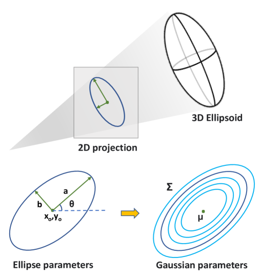
Figure 1: Top: We consider 2D projections of a 3D ellipsoid approximating the object. Bottom-left: Standard ellipse representation with centre coordinates ($x_{0},y_{0}$), major ($a$) and minor ($b$) axes, and orientation $\theta$. Bottom-right: To cope with the discontinuity of $\theta$, we propose to represent the ellipse by an underlying implicit Gaussian distribution parameterized by both continuous mean $\mu=\left(x_{0},y_{0}\right)$ and covariance $\Sigma=\begin{pmatrix}\mathrm{cos}(\theta)&-\mathrm{sin}(\theta)\\ \mathrm{sin}(\theta)&\mathrm{cos}(\theta)\end{pmatrix}\begin{pmatrix}a^{2}&0\\ 0&b^{2}\end{pmatrix}\begin{pmatrix}\mathrm{cos}(\theta)&\mathrm{sin}(\theta)\\ -\mathrm{sin}(\theta)&\mathrm{cos}(\theta)\end{pmatrix}$.

Gaussian Proposal Networks (GPN) [5], inspired by Region Proposal Networks (RPN) [6], look at ellipses as 2D Gaussian distributions on the image plane and minimizes the Kullback-Leibler (KL) divergence between the proposed and groundtruth distributions as one single loss. Since KL divergence has an analytical form for Gaussians and is differentiable, GPN can be easily implemented and trained with a back-propagation algorithm. However, the Gaussian parameters are derived from the regressed geometric parameters (position, axes and orientation), therefore facing the same discontinuity issue on angle regression. GPN has been integrated into an object detection pipeline by Pan et al. [7], where the Wasserstein metric is used instead of KL to provide the model with proper distance loss. Ellipse R-CNN [2] also regresses geometric ellipse parameters with enhanced occlusion robustness, while ElDet [8] adds training objectives such as maximizing Intersection-over-Union (IoU) score between predicted and groundtruth ellipses. However, these methods are designed to detect naturally occurring elliptic shapes in images, which does not correspond to our use-case, where ellipses originate from a 3D virtual ellipsoid modeling the object.

3D-Aware Ellipse Regression To the best of our knowledge, Zins et al. [9, 10, 11] were the first ones to regress 3D-aware ellipses. In [9], they apply a L2 loss on the ellipse centre and dimensions, while the angle prediction is framed as a classification problem with posterior angular correction loss. They also proposed two types of implicit functions characterized by ellipse parameters for robustifying the loss function: a local signed distance function enabling pixel-to-pixel comparison between groundtruth and predicted functions values [10] and an algebraic distance function based on ellipse equation combined with an adaptive sampling to provide rotation invariance [11]. However, implicit function values are still computed based on the regressed geometric ellipse parameters.

In this paper, we take up this implicit function idea but propose to continuously regress its values over the image pixels in the form of an occupancy heatmap. Before training, the Gaussian distribution parameters and heatmaps are directly computed from the ellipsoid projections using the relative object-camera poses. We extract these parameters from the regressed heatmap during forward propagation thanks to a novel non-trainable differentiable layer: Extended-Differentiable Spatial to Numerical Transform (E-DSNT). A combination of statistical losses is finally proposed to optimize the model. Though our method can be used in any use-case requiring 2D target localization, we focus on the Space Situational Awareness (SSA) application to validate it in this paper. Indeed, automatically localizing a target uncooperative spacecraft is crucial for tasks such as in-orbit rendezvous. We evaluated our work on three spacecraft pose estimation benchmark datasets. In a nutshell, our contributions are three-fold:

• A novel and fully differentiable object localization pipeline that can regress 3D-aware ellipse labels directly from an image. This proposed approach achieves state-of-the-art performance on standard spacecraft localization benchmarks;

• A method for generating 3D-aware Gaussian occupancy labels given only 6-Degree-of-Freedom relative poses and coarse object dimensions;

• An open-access release of 3D-aware Gaussian occupancy labels (heatmaps, mean and covariance labels) for three existing spacecraft pose estimation datasets.

The organization of the rest of the paper is as follows. Section II describes the generation of 3D-aware Gaussian occupancy labels for object localization in images. Section III presents our object Localization model designed to regress such labels. Then, experimental comparisons demonstrating the state-of-the-art performance of the method are provided in Section IV. Finally, Section V concludes the paper.

II 3D-AWARE GAUSSIAN OCCUPANCY LABELS

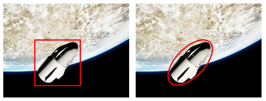
Figure 2: Illustration of bounding box object label (left) and ellipse label (right). The ellipse is a more accurate representation of many man-based objects. Image from the URSO Dataset [12].

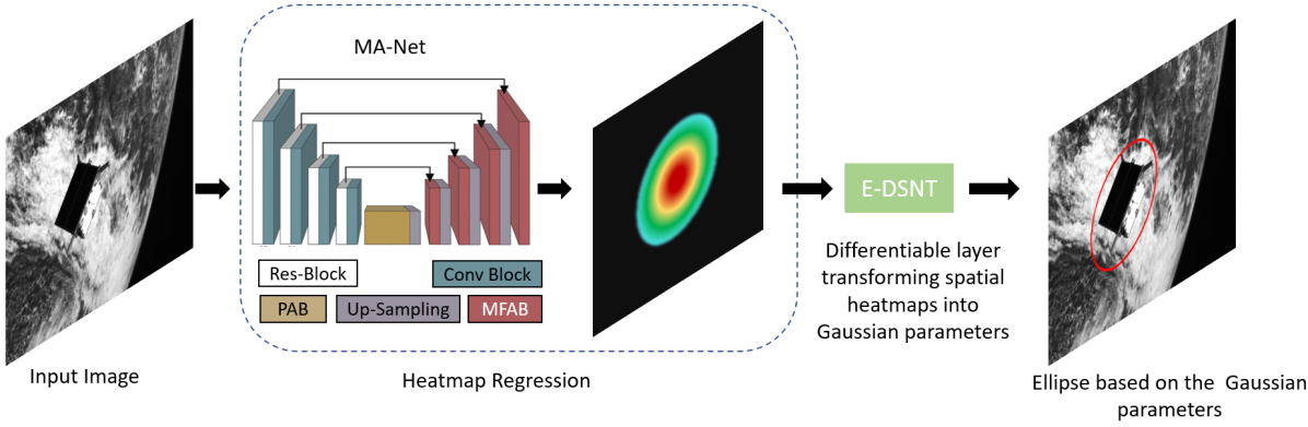
Figure 3: Illustration of our object localization pipeline designed to regress the parameters of a 3D-aware Gaussian implicit occupancy function (represented as a heatmap in the central picture) in a fully differentiable manner. The model combines an MA-Net backbone to regress the implicit function values over image pixels with a novel non-trainable differentiable layer (E-DSNT) to extract Gaussian distribution parameters. The corresponding ellipse is then derived (overlaid in red in the right picture). Image from the SPEED+ Dataset [13].

This section describes how to readily generate Gaussian occupancy labels from a 3D ellipsoidal model of the object and the relative camera-object pose.

II-A 2D Object Occupancy

Object occupancy in a picture can be defined as the set of pixels corresponding to that object. In most cases, object detection labels $L_{obj}$ are in the form of bounding boxes designed to encompass the object occupancy (see Fig. 2). Considering a bounding box with centre $(x_{c},y_{c})$ and dimensions $(W,H)$, object detection labels can be written:

$$L_{obj}^{(bbox)}=\left[x_{c},y_{c},W,H\right]\mbox{.}$$ (1)

Now assuming that the object occupancy is encoded by an implicit occupancy function $O_{\mathbf{p}}:\mathbb{R}^{2}\rightarrow\mathbb{R}$ characterized by parameters $\mathbf{p}$, object labels can be written

$$L_{obj}=\mathbf{p}\mbox{.}$$ (2)

II-B 2D Gaussian Occupancy Labels

Statistical information about the object occupancy is given by means $\mu_{x},\mu_{y}$, variances $\Sigma_{xx},\Sigma_{yy}$ and covariance $\Sigma_{xy}$ of the occupied pixels in the 2D image. Therefore, a natural implicit occupancy function is the bivariate Gaussian distribution with centre $\mathbf{\mu}=(\mu_{x},\mu_{y})^{\top}$ and covariance matrix $\Sigma=\begin{pmatrix}\Sigma_{xx}&\Sigma_{xy}\\ \Sigma_{xy}&\Sigma_{yy}\end{pmatrix}\mbox{.}$ Finally, we define Gaussian occupancy labels as

$$L_{obj}^{(Gauss)}=[\mu_{x},\mu_{y},\Sigma_{xx},\Sigma_{yy},\Sigma_{xy}]\mbox{.}$$ (3)

II-C 3D-Aware Gaussian Occupancy Labels

The parameters of a bivariate Gaussian distribution are those of a characteristic ellipse, and vice versa. In our method, we are interested in regressing the parameters of the elliptic projection of a 3D ellipsoid, and for this reason, we consider the Gaussian distribution arising from it.

More precisely, given an object whose dimensions along its three orthogonal principal directions are $2a^{\prime},2b^{\prime},2c^{\prime}$, an ellipsoidal approximation of the object is characterized by matrix

$$Q^{*}=diag\begin{pmatrix}a^{\prime 2}&b^{\prime 2}&c^{\prime 2}&-1\end{pmatrix}\mbox{.}$$ (4)

Then, denoting $\mathrm{T}$ the object centre position and $\mathrm{R}$ the object orientation with respect to the camera, the ellipsoid projection into the image (ellipse) is given by matrix

$$C^{*}=PQ^{*}P^{\top}\mbox{,}$$ (5)

where $P=\mathrm{K}\left[\mathrm{R}|\mathrm{T}\right]$ and $\mathrm{K}$ the camera intrinsic matrix [14].

The projected ellipse $C^{*}$ is therefore in the form:

$$C^{*}=s\begin{pmatrix}\cdot&\cdot&-x_{0}\\ \cdot&\cdot&-y_{0}\\ -x_{0}&-y_{0}&-1\end{pmatrix}\mbox{,}$$ (6)

where $s$ is a scale factor, $\cdot$ denotes any value, and $(x_{0},y_{0})$ is the ellipse centre that corresponds to the peak location of the underlying Gaussian occupancy function:

$$\mu=(\mu_{x},\mu_{y})^{\top}=(x_{0},y_{0})^{\top}\mbox{.}$$ (7)

The centred ellipse is then obtained by

$$C_{\mathrm{centered}}^{*}=TC^{*}T^{\top}\mbox{,}$$ (8)

where $T=\begin{pmatrix}1&0&-x_{0}\\ 0&1&-y_{0}\\ 0&0&1\end{pmatrix}\mbox{.}$

The $2\times 2$ upper-left part of $C_{\mathrm{centered}}^{*}$ corresponds to the covariance $\Sigma$ of the Gaussian occupancy function, and its eigendecomposition provides the ellipse orientation $\theta$ and semi-axes $(a,b)$:

$$\Sigma =\begin{pmatrix}\Sigma_{xx}&\Sigma_{xy}\\ \Sigma_{xy}&\Sigma_{yy}\end{pmatrix}$$ (9)

$$=\begin{pmatrix}\mathrm{cos}(\theta)&-\mathrm{sin}(\theta)\\ \mathrm{sin}(\theta)&\mathrm{cos}(\theta)\end{pmatrix}\begin{pmatrix}a^{2}&0\\ 0&b^{2}\end{pmatrix}\begin{pmatrix}\mathrm{cos}(\theta)&\mathrm{sin}(\theta)\\ -\mathrm{sin}(\theta)&\mathrm{cos}(\theta)\end{pmatrix}\mbox{.}$$ (10)

III OBJECT LOCALIZATION

Our object localization pipeline, illustrated in Fig.3, can regress Gaussian occupancy labels $L_{obj}^{(Gauss)}$ via implicit function estimation in a fully differentiable manner. We introduce a differentiable heatmap parameters extraction layer E-DSNT coupled with a heatmap regression network to estimate the implicit function values. These modules are respectively presented in Sections III-B and III-A. The statistical loss used to optimize the model is presented in Section III-C.

III-A Heatmap Regression Network

Any state-of-the-art segmentation network can be used to regress the Gaussian occupancy function values $O_{\mathbf{p}}(x,y)$ across image pixels. In the experiments, we use the MA-Net [15] network with ResNet34 [16] backbone since this model can capture contextual dependencies based on an attention mechanism, using two blocks (refer to Fig.3): a Position-wise Attention Block (PAB), which captures the spatial dependencies between pixels in a global view, and a Multi-scale Fusion Attention Block (MFAB), which captures the channel dependencies between any feature map by multi-scale semantic feature fusion. As a last layer, a flattening-softmax layer is added to ensure a normalized probability density function, which we refer to as a heatmap in what follows.

III-B Differentiable Extraction of Gaussian Occupancy Labels

A bivariate Gaussian distribution is characterized by its mean value $\mu$, being the coordinates of the peak, and its covariance matrix $\Sigma$ encoding the spatial extent of the distribution. A differentiable mean extraction layer was previously introduced in the literature (see Section III-B1), and we extend it to extract the additional covariance matrix values, refer to Section III-B2.

III-B1 Mean Extraction

Differentiable Spatial to Numerical Transform (DSNT) [17] is a non-trainable and differentiable layer for extracting the mean value of a given normalized Gaussian heatmap $\hat{Z}$ with size $H\times W$. Following this method, we compute two coordinates encoding matrices $X$ and $Y$ with entries

$$\begin{split}X_{i,j}=\frac{2j-(W+1)}{W}\mbox{;}\hskip 5.69046ptY_{i,j}=\frac{2i-(H+1)}{H}\mbox{,}\\ \forall i=1,\ \dots,\ H\mbox{;}\hskip 5.69046pt\forall j=1,\ \dots,\ W\mbox{.}\end{split}$$

Observing that the heatmap encodes the probability $P$ of the pixel $\left[X_{i,j}\mbox{ , }Y_{i,j}\right]$ to be the location of the peak $p$, we have:

$$\begin{split}P(p=[X_{i,j}\mbox{ , }Y_{i,j}])=\hat{Z}_{i,j}\mbox{.}\end{split}$$

The prediction of $p$ is made through its expectation

$$\begin{split}\mu=\mathbb{E}[p]=\left[<\hat{Z},X>_{F}\quad<\hat{Z},Y>_{F}\right]\end{split}$$ (11)

where $<\cdot,\cdot>_{F}$ is the Frobenius inner product.

III-B2 Covariance Matrix Extraction

Denoting $p_{x},p_{y}$ the coordinates of $p$, we extend DSNT to extract the heatmap variances along the x-axis $\Sigma_{xx}$ and y-axis $\Sigma_{yy}$, as well as its covariance value $\Sigma_{xy}$. We refer to such parameter extraction procedure as Extended-DSNT (E-DSNT). Specifically, we use the definitions of the aforementioned quantities and derive the following equations:

$$\begin{split}\Sigma_{xx}&=\mathbb{E}[(p_{x}-\mathbb{E}[p_{x}])^{2}]\\ &=<\hat{Z},(X-\mu_{x})\odot(X-\mu_{x})>_{F}\end{split}$$ (12)

$$\begin{split}\Sigma_{yy}&=\mathbb{E}[(p_{y}-\mathbb{E}[p_{y}])^{2}]\\ &=<\hat{Z},(Y-\mu_{y})\odot(Y-\mu_{y})>_{F}\end{split}$$ (13)

$$\begin{split}\Sigma_{xy}&=\mathbb{E}[(p_{x}-\mathbb{E}[p_{x}])(p_{y}-\mathbb{E}[p_{y}])]\\ &=<\hat{Z},(X-\mu_{x})\odot(Y-\mu_{y})>_{F}\end{split}$$ (14)

Therefore, the Gaussian distribution parameters are the centre $\mu$, obtained from Eq. (11), and the covariance matrix $\Sigma$ formed by left terms of Eq. (12), (13) and (14).

III-B3 Ellipse Parameters Computation

The centre of the ellipse is simply $\left(x_{0},y_{0}\right)=\mu$. Its axes $a,b$ and orientation $\theta$ are obtained by the eigendecomposition of the covariance matrix $\Sigma$ (see Eq. 10).

III-C Model Loss

Our loss $\mathcal{L}$ can be written as a combination of two losses. We use the Wasserstein distance $\mathcal{L}_{\mathrm{W}}$ to directly optimize the Gaussian parameters, while the Jensen-Shannon divergence $\mathcal{L}_{\mathrm{JS}}$, applied on the heatmap values, is used to regularize the implicit occupancy function $O_{\mathbf{p}}$. Our loss is then

$$\mathcal{L}=\mathcal{L}_{\mathrm{W}}+\lambda.\mathcal{L}_{\mathrm{JS}}\mbox{,}$$ (15)

with a scalar factor $\lambda$ to balance the two losses.

In details, considering predicted and groundtruth Gaussian distributions $\mathcal{G}_{\mathrm{pd}}$ and $\mathcal{G}_{\mathrm{gt}}$ characterized by means and covariances $(\mu_{\mathrm{pd}},\Sigma_{\mathrm{pd}})$ and $(\mu_{\mathrm{gt}},\Sigma_{\mathrm{gt}})$, the Wasserstein distance term is given by:

$$\begin{split}\mathcal{L}_{\mathrm{W}}=&\mbox{ }d_{W}(\mathcal{G}_{\mathrm{pd}},\mathcal{G}_{\mathrm{gt}})\\ =&\left|\left|\mu_{\mathrm{pd}}-\mu_{\mathrm{gt}}\right|\right|_{2}^{2}+\mathrm{tr}\left(\Sigma_{\mathrm{pd}}+\Sigma_{\mathrm{gt}}-2\left(\Sigma_{\mathrm{gt}}^{\frac{1}{2}}\Sigma_{\mathrm{pd}}\Sigma_{\mathrm{gt}}^{\frac{1}{2}}\right)^{\frac{1}{2}}\right)\mbox{.}\end{split}$$ (16)

Such closed-form expression avoids relying on handcrafted relative weights to balance the contributions of mean, variance and covariance terms.

The Jensen-Shannon divergence term is defined as:

$$\mathcal{L}_{\mathrm{JS}}=\frac{1}{2}D_{\mathrm{KL}}(\mathcal{G}_{\mathrm{pd}}\|\mathcal{G}_{\mathrm{m}})+\frac{1}{2}D_{\mathrm{KL}}(\mathcal{G}_{\mathrm{gt}}\|\mathcal{G}_{\mathrm{m}})\mbox{,}$$ (17)

where $\mathcal{G}_{\mathrm{m}}=\frac{1}{2}(\mathcal{G}_{\mathrm{pd}}+\mathcal{G}_{\mathrm{gt}})$ and $D_{\mathrm{KL}}(\mathcal{D}_{1}\|\mathcal{D}_{2})$ is the Kullback-Leibler divergence between any distributions $\mathcal{D}_{1}$ and $\mathcal{D}_{2}$, given by

$$D_{\mathrm{KL}}(\mathcal{D}_{1}\|\mathcal{D}_{2})=\sum_{(i,j)\in I}\mathcal{D}_{1}(i,j)\mbox{ }\mathrm{log}\left(\frac{\mathcal{D}_{1}(i,j)}{\mathcal{D}_{2}(i,j)}\right)\mbox{.}$$ (18)

That term is computed directly from the implicit function values over pixels ($i,j$) of heatmap $I$. The Jensen-Shannon divergence has the advantage of being symmetric, in contrast with Kullback-Leibler, and it has been proven to perform better than the latter in [17].

IV EXPERIMENTS AND DISCUSSION

	IoU ($\uparrow$)	Overlap ($\uparrow$)	Dice ($\uparrow$)	RVD ($\downarrow$)	MHD ($\downarrow$)
Rubino et al. [18]	0.78$\pm$0.06	0.93$\pm$0.04	0.88$\pm$0.04	0.12$\pm$0.08	6.88$\pm$5.98
Zins et al. [10]	0.91$\pm$0.12	0.96$\pm$0.07	0.95$\pm$0.08	0.02$\pm$0.04	3.93$\pm$5.63
Ours ($\mathcal{L}_{\mathrm{W}}$)	0.89$\pm$0.05	0.98$\pm$0.02	0.94$\pm$0.03	0.08$\pm$0.06	3.48$\pm$1.80
Ours ($\mathcal{L}_{\mathrm{W}}+\mathcal{L}_{\mathrm{JS}}$)	0.93$\pm$0.03	0.97$\pm$0.02	0.96$\pm$0.01	0.01$\pm$0.01	2.16$\pm$0.66
Ours ($\mathcal{L}_{\mathrm{JS}}$)	0.93$\pm$0.03	0.97$\pm$0.02	0.96$\pm$0.02	0.01$\pm$0.01	2.26$\pm$0.77

TABLE I: Experimental validation on AKM [19] dataset. Best results are in bold.

	IoU ($\uparrow$)	Overlap ($\uparrow$)	Dice ($\uparrow$)	RVD ($\downarrow$)	MHD ($\downarrow$)
Rubino et al. [18]	0.70$\pm$0.13	0.91$\pm$0.10	0.82$\pm$0.13	0.17$\pm$0.17	88.35$\pm$119.49
Zins et al. [10]	0.85$\pm$0.18	0.95$\pm$0.12	0.91$\pm$0.15	0.07$\pm$0.15	54.38$\pm$116.38
Ours ($\mathcal{L}_{\mathrm{W}}$)	0.82$\pm$0.09	0.95$\pm$0.05	0.90$\pm$0.06	0.08$\pm$0.13	9.59$\pm$7.18
Ours ($\mathcal{L}_{\mathrm{W}}+\mathcal{L}_{\mathrm{JS}}$)	0.86$\pm$0.08	0.95$\pm$0.05	0.92$\pm$0.05	0.03$\pm$0.06	7.85$\pm$6.86
Ours ($\mathcal{L}_{\mathrm{JS}}$)	0.87$\pm$0.07	0.95$\pm$0.04	0.93$\pm$0.05	0.01$\pm$0.05	7.58$\pm$6.89

TABLE II: Experimental validation on SPEED+ [13] dataset. Best results are in bold.

Datasets Extension with 3D-Aware Gaussian Occupancy Labels We have extended three public spacecraft pose estimation datasets with Gaussian occupancy labels. SPEED [20] and SPEED+ [13] are the standard benchmarks for spacecraft pose estimation methods, while AKM [21] is a recently released dataset featuring texture-less and symmetrical space objects [22]. No CAD data is available in the first two datasets, but our method requires only the coarse dimensions of the considered spacecraft (TANGO dimensions: 80$\times$75$\times$32cm [23]).

Object Localization Metrics Our metrics are the Intersection-over-Union score (denoted by IoU), the Overlap score (Overlap), the Dice-Sorensen coefficient (Dice), the Relative Volume Difference (RVD) and the Modified Hausdorff Distance (MHD) [24]. Denoting $P$ and $G$ the sets of pixels inside predicted and groundtruth ellipses, the metrics are defined as

$$\mathrm{IoU}=\frac{\mathrm{area}(P\cap G)}{\mathrm{area}(P\cup G)}\mbox{,}$$ (19)

$$\mathrm{Overlap}=\frac{\mathrm{area}(P\cap G)}{\mathrm{min}(\mathrm{area}(P),\mathrm{area}(G))}\mbox{,}$$ (20)

$$\mathrm{Dice}=2\frac{\mathrm{area}(P\cap G)}{\mathrm{area}(P)+\mathrm{area}(G)}\mbox{,}$$ (21)

$$\mathrm{RVD}=\frac{|\mathrm{area}(P)-\mathrm{area}(G)|}{\mathrm{area}(G)}\mbox{.}$$ (22)

While these four metrics characterize in different ways the discrepancy between regions $P$ and $G$ bounded by predicted and groundtruth ellipses, MHD [24] direclty measures the discrepancy between the (discretized) ellipses $\partial P$ and $\partial G$:

$$\mathrm{MHD}=\mathrm{max}\left(\mathrm{mhd}(\partial P,\partial G),\mathrm{mhd}(\partial G,\partial P)\right)\mbox{,}$$ (23)

where $\mathrm{mhd}(.)$ is the relative modified Hausdorff distance:

$$\mathrm{mhd}(\partial P,\partial G)=\frac{1}{|\partial P|}\sum_{p\in\partial P}\min_{g\in\partial G}(\|p-g\|_{2})$$ (24)

in which $p$ and $g$ denote points on the respective discretized ellipses (total number of points for ellipse $\partial P$: $|\partial P|$).

Considering these five metrics allows for a fairly extensive comparison between the performance of different ellipse prediction methods.

Baselines Given a 3D object modelled by an ellipsoid, our method aims at regressing its elliptic projections in the pictures. We provide a qualitative and quantitative comparison with two other representative 3D-aware ellipse regression methods. It is important noting that most 2D ellipse regression methods [3, 4, 5, 6, 7, 2, 8] are, by contrast, to detect naturally occurring 2D elliptic shapes in images. The first baseline, from Zins et al. [10], is a 2-stage approach consisting in localizing the object using an object detector (Faster R-CNN [6] with ResNet50 [25] backbone in the official implementation), then regressing the geometric ellipse parameters from the cropped image. This method is an improved version of their previous work [9]. The second approach, used in most ellipsoid-based pose estimation problems (e.g.,  [18]), consists in fitting an axis-aligned ellipse within the detected bounding box (same detection model in the experiments).

Object Localization Results Tables I and II show a comparison between our model optimized with Wasserstein loss only, Jensen-Shannon loss only and a combination of both ($\lambda=1$), along with methods from Rubino et al. [18] and Zins et al. [10]. It shows that our method, even if relying on a lighter backbone (ResNet32), outperforms its competitors on AKM and SPEED+ datasets for each of the five metrics. For our model on AKM dataset, both losses leveraging Jensen-Shannon divergence achieve the same level of accuracy, suggesting that the most important optimization factor is the implicit function regularization. On SPEED+, the model trained only with Jensen-Shannon divergence obtained the best performance because the Gaussian implicit function is slightly truncated outside image boundaries, thus misleading the parameters extraction.

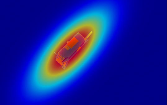
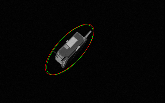
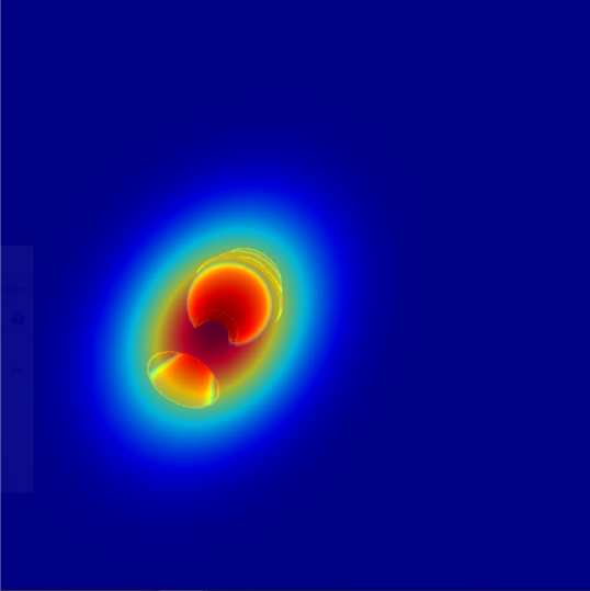
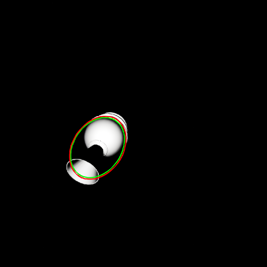
Figure 4: Qualitative results on SPEED+ (top) and AKM (bottom) datasets. Implicit occupancy functions from regressed parameters overlaid as heatmaps (left), with extracted (red) and groundtruth (green) ellipses (right).

In addition, our 1-stage approach has the advantage of performing localization and parameter extraction simultaneously in a fully differentiable manner. Moreover, the parameters extraction is performed by the novel E-DSNT non-trainable layer, hence resulting in a lighter model. Finally, it avoids regressing a discontinuous angular parameter (ellipse orientation), unlike [9, 10] and all other ellipse detection methods. Qualitative results, presented in Fig. 4, show the implicit occupancy function values, groundtruth and predicted ellipses.

3D Reconstruction To assess the 3D-awareness of our predictions, we use regressed ellipse parameters as inputs to a 3D ellipsoid reconstruction method based on triangulation of 2D ellipses [18]. We randomly selected 100 images from the SPEED+ dataset and reconstructed the ellipsoid based on the ellipses regressed from the different methods. Figure 5 shows that the ellipsoid reconstructed from our predictions (in red) is closer to the groundtruth ellipsoid (green) than those obtained from other methods (blue, magenta). Quantitatively, an evaluation conducted over 200 subsets of 50 random images is provided in Table III. It shows that our method allows for the most accurate reconstruction, demonstrating the 3D awareness of our regressed ellipses, which is of particular importance for a possibly following 6 Degrees-of-Freedom (6DoF) object pose estimation task [26, 27].

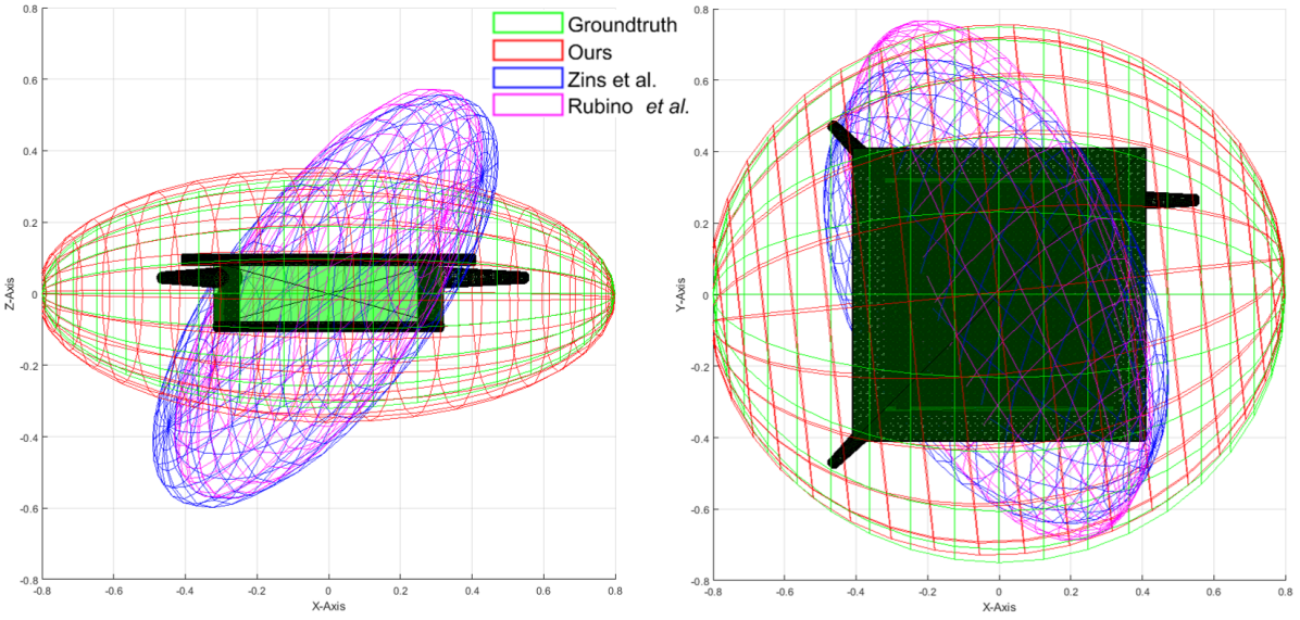
Figure 5: Illustration of TANGO spacecraft (SPEED+ dataset) with groundtruth (in green) and reconstructed ellipsoids from our method (red), Zins et al. [9] (blue) and Rubino et al. [18] (magenta). The reconstruction method is from [18]. The ellipsoid reconstructed from our predictions is closer to the groundtruth ellipsoid than those obtained from other methods.

	Position	Orientation	Size
Rubino et al. [18]	5.9cm	10.2$\degree$	11.0cm
Zins et al. [10]	2.1cm	4.1$\degree$	8.0cm
Ours ($\mathcal{L}_{\mathrm{JS}}$)	1.0cm	0.1$\degree$	2.4cm

TABLE III: 3D reconstruction errors on SPEED+ [13] dataset, using ellipse triangulation method [18]. Best results are in bold.

V CONCLUSION

In this paper, we presented a fully differentiable 3D-aware object localization method based on Gaussian implicit occupancy function and ellipse labels. We explained how to readily generate consistent Gaussian occupancy labels to extend already existing pose datasets without requiring any CAD model of the object. We also release the labels for three public spacecraft pose estimation datasets. Future work will focus on integrating that 2D localization model into an end-to-end 6DoF spacecraft pose estimation pipeline, and evaluate on real datasets [13, 28].

References

- [1] L. Liu, W. Ouyang, X. Wang, P. Fieguth, J. Chen, X. Liu, and M. Pietikäinen, “Deep learning for generic object detection: A survey,” Int. J. Comput. Vis., vol. 128, no. 2, pp. 261–318, 2020.
- [2] W. Dong, P. Roy, C. Peng, and V. Isler, “Ellipse R-CNN: learning to infer elliptical object from clustering and occlusion,” IEEE Trans. Image Process., vol. 30, pp. 2193–2206, 2021.
- [3] Z. Wang, N. Dong, S. D. Rosario, M. Xu, P. Xie, and E. P. Xing, “Ellipse detection of optic disc-and-cup boundary in fundus images,” in 16th IEEE International Symposium on Biomedical Imaging (ISBI), 2019, pp. 601–604.
- [4] H. Lin, Z. Li, M. Shih, Y. Sun, and T. Shen, “Pupil localization for ophthalmic diagnosis using anchor ellipse regression,” in 16th International Conference on Machine Vision Applications (MVA), 2019, pp. 1–5.
- [5] Y. Li, “Detecting lesion bounding ellipses with gaussian proposal networks,” in MICCAI Workshops 2019, Proceedings. Springer, 2019, pp. 337–344.
- [6] S. Ren, K. He, R. B. Girshick, and J. Sun, “Faster R-CNN: towards real-time object detection with region proposal networks,” in NIPS, 2015, pp. 91–99.
- [7] S. Pan, S. Fan, S. W. K. Wong, J. V. Zidek, and H. Rhodin, “Ellipse detection and localization with applications to knots in sawn lumber images,” in IEEE Winter Conference on Applications of Computer Vision (WACV), 2021, pp. 3891–3900.
- [8] T. Wang, C. Lu, M. Shao, X. Yuan, and S. Xia, “Eldet: An anchor-free general ellipse object detector,” in Proceedings of the Asian Conference on Computer Vision (ACCV), 2022, pp. 2580–2595.
- [9] M. Zins, G. Simon, and M.-O. Berger, “3d-aware ellipse prediction for object-based camera pose estimation,” in 8th International Conference on 3D Vision, 3DV 2020. IEEE, 2020, pp. 281–290.
- [10] ——, “Object-based visual camera pose estimation from ellipsoidal model and 3d-aware ellipse prediction,” International Journal of Computer Vision, vol. 130, no. 4, pp. 1107–1126, 2022.
- [11] ——, “Level set-based camera pose estimation from multiple 2d/3d ellipse-ellipsoid correspondences,” in IEEE/RSJ International Conference on Intelligent Robots and Systems (IROS), 2022.
- [12] P. F. Proença and Y. Gao, “Deep learning for spacecraft pose estimation from photorealistic rendering,” in IEEE International Conference on Robotics and Automation, (ICRA), 2020, pp. 6007–6013.
- [13] T. H. Park, M. Märtens, G. Lecuyer, D. Izzo, and S. D’Amico, “Speed+: Next-generation dataset for spacecraft pose estimation across domain gap,” in IEEE Aerospace Conference (AERO), 2022, pp. 1–15.
- [14] R. I. Hartley and A. Zisserman, Multiple View Geometry in Computer Vision, 2nd ed. Cambridge University Press, 2004.
- [15] T. Fan, G. Wang, Y. Li, and H. Wang, “Ma-net: A multi-scale attention network for liver and tumor segmentation,” IEEE Access, vol. 8, pp. 179 656–179 665, 2020.
- [16] K. He, X. Zhang, S. Ren, and J. Sun, “Deep residual learning for image recognition,” in Proceedings of the IEEE Conference on Computer Vision and Pattern Recognition (CVPR), June 2016.
- [17] A. Nibali, Z. He, S. Morgan, and L. Prendergast, “Numerical coordinate regression with convolutional neural networks,” arXiv preprint arXiv:1801.07372, 2018.
- [18] C. Rubino, M. Crocco, and A. Del Bue, “3d object localisation from multi-view image detections,” IEEE Transactions on Pattern Analysis and Machine Intelligence, vol. 40, no. 6, pp. 1281–1294, 2018.
- [19] A. Rathinam, V. Gaudilliere, L. Pauly, and D. Aouada, “AKM Dataset: Textureless Space Target Dataset,” https://zenodo.org/record/7744505, Sep 2022.
- [20] M. Kisantal, S. Sharma, T. H. Park, D. Izzo, M. Märtens, and S. D’Amico, “Satellite pose estimation challenge: Dataset, competition design, and results,” IEEE Trans. Aerosp. Electron. Syst., vol. 56, no. 5, pp. 4083–4098, 2020.
- [21] A. Rathinam, V. Gaudillière, L. Pauly, and D. Aouada, “Pose Estimation of a Known Texture-Less Space Target using Convolutional Neural Networks,” in 73th International Astronautical Congress (IAC), 2022.
- [22] L. Pauly, W. Rharbaoui, C. Shneider, A. Rathinam, V. Gaudillière, and D. Aouada, “A survey on deep learning-based monocular spacecraft pose estimation: Current state, limitations and prospects,” ArXiv preprint, vol. abs/2305.07348, 2023. [Online]. Available: https://doi.org/10.48550/arXiv.2305.07348
- [23] S. M. Catalogue, “Prisma (prototype),” https://www.eoportal.org/satellite-missions/prisma-prototype#target-spacecraft.
- [24] M.-P. Dubuisson and A. Jain, “A modified hausdorff distance for object matching,” in Proceedings of 12th International Conference on Pattern Recognition, vol. 1, 1994, pp. 566–568.
- [25] K. He, X. Zhang, S. Ren, and J. Sun, “Deep residual learning for image recognition,” in 2016 IEEE Conference on Computer Vision and Pattern Recognition (CVPR), 2016, pp. 770–778.
- [26] A. Garcia, M. A. Musallam, V. Gaudillière, E. Ghorbel, K. Al Ismaeil, M. Perez, and D. Aouada, “Lspnet: A 2d localization-oriented spacecraft pose estimation neural network,” in Proceedings of the IEEE/CVF Conference on Computer Vision and Pattern Recognition, 2021, pp. 2048–2056.
- [27] V. Gaudillière, G. Simon, and M.-O. Berger, “Perspective-1-ellipsoid: Formulation, analysis and solutions of the camera pose estimation problem from one ellipse-ellipsoid correspondence,” International Journal of Computer Vision, vol. 131, no. 9, pp. 2446–2470, 2023.
- [28] A. Rathinam, V. Gaudillière, M. A. Mohamed Ali, M. Ortiz Del Castillo, L. Pauly, and D. Aouada, “SPARK 2022 Dataset : Spacecraft Detection and Trajectory Estimation,” June 2022. [Online]. Available: https://doi.org/10.5281/zenodo.6599762