Abstract

We present the first calibration of quantum decision theory (QDT) to a dataset of binary risky choice. We quantitatively account for the fraction of choice reversals between two repetitions of the experiment, using a probabilistic choice formulation in the simplest form without model assumption or adjustable parameters. The prediction of choice reversal is then refined by introducing heterogeneity between decision makers through their differentiation into two groups: “majoritarian” and “contrarian” (in proportion 3:1). This supports the first fundamental tenet of QDT, which models choice as an inherent probabilistic process, where the probability of a prospect can be expressed as the sum of its utility and attraction factors. We propose to parameterise the utility factor with a stochastic version of cumulative prospect theory (logit-CPT), and the attraction factor with a constant absolute risk aversion (CARA) function. For this dataset, and penalising the larger number of QDT parameters via the Wilks test of nested hypotheses, the QDT model is found to perform significantly better than logit-CPT at both the aggregate and individual levels, and for all considered fit criteria for the first experiment iteration and for predictions (second “out-of-sample” iteration). The distinctive QDT effect captured by the attraction factor is mostly appreciable (i.e., most relevant and strongest in amplitude) for prospects with big losses. Our quantitative analysis of the experimental results supports the existence of an intrinsic limit of predictability, which is associated with the inherent probabilistic nature of choice. The results of the paper can find applications both in the prediction of choice of human decision makers as well as for organizing the operation of artificial intelligence.

Keywords: Quantum decision theory, Prospect probability, Utility factor, Attraction factor, Stochastic cumulative prospect theory, Predictability limit

1 Introduction

The life of every human being (and even of almost every alive being) is a permanent chain of decisions and actions resulting from these decisions. There are two types of decisions: Individual decisions taken by separate individuals without consulting others, and collective decisions accepted after discussions with other involved individuals. Humans are social animals and many their decisions are collective, being influenced by social relations [1, 2, 3]. Nevertheless, the first step in developing any decision theory is the characterization of individual decision making.

There exist several variants of decision theory, whose peculiarities and limitations are discussed below. An original approach in decision theory, called quantum decision theory (QDT) has been advanced by the authors [4]. The idea of this approach is the use of techniques of quantum theory for describing the complex structure of realistic decisions containing the rational reasoning as well as irrational emotional parts. It turns out that this rational-irrational duality can be successfully described by quantum techniques developed for characterizing the theory of quantum measurements. At the same time, mathematics of quantum theory is just a convenient tool not requiring that decision makers be in any sense quantum devices. After understanding the pivotal technical points of the approach, it is possible to reformulate the basic concepts so that it would be straightforward to employ the approach without resorting to quantum terminology. This concerns the main content of the present paper, whose reading does not need any knowledge of quantum theory. Quantum analogies and foundations are mentioned in Appendix and can be neglected by those who are not acquainted with quantum notions.

The QDT approach can be applied to individual as well as to collective decision making, when agents form a society and repeatedly exchange information between each other [5, 6, 7]. However, the ultimate aim is not merely qualitatively describe the novel approach in decision theory but to develop it to the level allowing for its use in practical problems needing rather accurate quantitative predictions. This paper is the first such an attempt of calibrating QDT, opening the ways for the following practical usage of the approach.

The principal goal of decision theory is to understand and predict the choices of decision makers, in particular when the decisions involve risky options. “Classical” economists use the Homo economicus assumption that decision making is the deterministic process of maximising an expected utility [8, 9, 10]. This formulation has been shown to lead to many paradoxes when confronted with real human decision makers.

Observed issues of “classical” models can be generalized into two classes:

• systematic deviations of behavior from predictions based on the expected utility, which led to a proliferation of behavioral models;

• choice variability over time, which gave rise to probabilistic extensions of deterministic models.

Systematic studies of behavioural patterns, revealed by accumulated empirical data, indicate violation of the classical axioms. These violations include: (a) common consequence and common ratio effects, which are inconsistent with the axiom of independence from irrelevant alternatives [11]; (b) the preference reversal phenomenon [12, 13] that is associated with a failure of procedure invariance and the axiom of transitivity [14]; and (c) framing effects as a breakdown of descriptive invariance [15]. Many models have been introduced to explain and predict observed cognitive and emotional biases [16, 17]. A number of theories have been advanced, such as prospect theory [18, 19, 20], rank-dependent utility theory [22, 21], cumulative prospect theory [23], configural weight models [24, 25], regret theory [27, 26], maximin expected utility model [28], Choquet expected utility model [29, 30] and many others. However, various attempts to extend utility theory by constructing non-expected utility functionals do not avoid common pitfalls in modeling risk aversion [31], cannot in general resolve the known classical paradoxes such as the conjunction fallacy, disjunction effect, and were criticized for employing ambiguity aversion to rationalize Ellsberg choices [32]. Moreover, extending the classical utility theory has been claimed “ending up creating more paradoxes and inconsistencies than it resolves” [32].

The observed variability of choice over time for one decision maker motivated the development of probabilistic extensions of deterministic “classical” models. The need to prioritise the advancement of research concerned with probabilistic descriptions, as compared to the development of new versions of deterministic behavioural models, has been pointed out for example in [34, 33, 35]. In fact, the axiomatic expected utility theory, when extended to incorporate truncated random errors, has been demonstrated to explain experimental data at least as well as cumulative prospect theory [36]. At the same time, the assumptions behind the stochasticity of choices have a wide range of interpretations, from erroneous and noisy execution to a useful evolutionarily feature, or left implicit. Moreover, different probabilistic specifications for the same core (deterministic) model have been shown to produce opposite predictions [34, 37, 39, 40, 38]. We review this topic in the next section.

Thus, modifications of “classical” models, by incremental additions of behavioral parameters and stochastic elements, had led to an impressive growth of the literature and of its complexity, without however convergence towards a commonly accepted solution for the two classes of paradoxes.

In the last decade, there has been a growing interest in a conceptually new way of modeling decisions by employing a toolbox that was originally developed for quantum mechanics. Within the “quantum” approach, decision making is seen as a process of deliberation between interfering choice options (prospects) with a probabilistic result, i.e. a probabilistic decision. Thus, it provides a parsimonious explanation for both modeling issues: systematic deviations from a rational choice criterion considered in isolation appear, unconsciously or intentionally, due to the presence and certain formulation of interconnected prospects. And the observed choice stochasticity is a manifestation of the inherently probabilistic nature of decision making.

The factors causing interference effects in decision processes include subjective and subconscious processes in the decision maker’s mind associated with available prospects coexisting with the prospect(s) under scrutiny for a decision action. This includes memories of past experiences, beliefs and momentary influences. All these operations in the mind of the decision maker may contribute to the existence of interferences between the different prospects and/or between a given prospect and his/her state of mind. In the Appendix summarising quantum decision theory, such interference effects are quantified by the attraction factor, which is one of the main objects of quantitative investigation in the present work.

The quantum decision theory that we follow here was first introduced in Ref. [4], with the goal of establishing a holistic theoretical framework of decision making. Based on the mathematics of Hilbert spaces, it provides a convenient formalism to deal with (real world) uncertainty and employs non-additive probabilities for the resolution of complex choice situations with interference effects. The use of Hilbert spaces constitutes the simplest generalization of the probability theory axiomatized by [41] for real-valued probabilities to probabilities derived from algebraic complex number theory. By its mathematical structure, quantum decision theory aims at encompassing the superposition processes occurring down to the neuronal level. This becomes especially important for composite (uncertain) measurements, with a formulation that differs from the diverse forms of probabilistic choice theory, including random preference models (mixture models), as the summary presentation of quantum decision theory in the Appendix should help comprehend. Numerous behavioural patterns, including those causing paradoxes within other theoretical approaches, are coherently explained by quantum decision theory [4, 42, 43, 44, 45, 48, 46, 47].

There are several alternative versions of quantum approach to decision making, which have been proposed in the literature, as seen for instance with the books [50, 51, 49] and the review articles [42, 54, 53, 52], where citations to the previous literature can be found. The version of Quantum Decision Theory (henceforth referred to as QDT), developed in Refs. [4, 42, 43, 44, 45, 48, 46, 47] and used here, principally differs from all other “quantum” approaches in two important aspects. First, QDT is based on a self-consistent mathematical foundation that is common to both quantum measurement theory and quantum decision theory. Starting from the theory of quantum measurements of von Neumann [55], the authors have generalized it to the case of uncertain or inconclusive events, making it possible to characterize uncertain measurements and uncertain prospects. Second, the main formulas of QDT are derived from general principles, giving the possibility of general quantitative predictions. In a series of papers [4, 42, 43, 44, 45, 48, 46, 47] the authors have compared a number of predictions with empirical data, without fitting parameters [44, 45, 46, 47]. This is in contrast with the other “quantum approaches” by other researchers consisting in constructing particular models for describing some specific experiments, with fitting the model parameters from experimental data.

Until now, predictions of QDT were made at the aggregate level, non parametrically and assuming no prior information. The present study intends to overcome these limitations, by developing a first parametric analytical formulation of QDT factors, enlarging the area of practical application of the theory and enabling higher granularity of predictions at both aggregate and individual levels.

For the first time, we engage QDT in a competition with decision making models, based on a mid size raw experimental data set of individual choices. The experiment was iterated twice (henceforth referred to as time 1 and time 2) and consists of simple choice tasks between two gambles with known outcomes and corresponding probabilities (i.e. binary lotteries). The data analysis reveals an inherent choice stochasticity, adding to the existing evidences, and supporting the probabilistic approach of QDT.

As a classical benchmark, we consider a stochastic version of cumulative prospect theory (henceforth referred to as logit-CPT) that combines cumulative prospect theory (CPT) with the logit choice function. Note that other models associated with “classical” theories, such as expected value and expected utility theory, are nested within it. For review on tests of nested and especially non-nested hypotheses, see [56].

Within QDT, a decision maker, who is exposed to several options, can choose any of these prospects with a certain probability. Thus, each choice option is associated with a prospect probability, which can be calculated as a sum of two factors: utility and attraction. In this paper, for the parametric formulation of QDT, we adopt the stochastic CPT approach (logit-CPT) for the utility factor, and incorporate a constant absolute risk aversion (CARA) into the attraction factor. This allows us to separate aversion to extreme losses and transfer it into the attraction factor.

We estimate parameters of the logit-CPT model and the utility factor of our QDT model with the hierarchical Bayesian method, as implemented in [59, 58, 57] and in [60, 61], using identical data set as [57], which ensures straightforward model selection. The proposed QDT formulation is found to perform better at both aggregate and individual levels, and for all considered criteria of fit (time 1) and prediction (time 2). As expected, the most noticeable effect is achieved for prospects involving large losses, whereas the overall improvement is small on average.

The difficulty of achieving significant improvements in the prediction of human decisions, despite persistent attempts of different approaches, raises the question of the limit of predictability. We propose to rationalize quantitatively the limits of predictability of human choices in terms of the inherent stochastic nature of choice, which implies that the fraction of correctly predicted decisions is also a random variable. We thus propose a theoretical distribution of the individual predicted fractions, and compare it successfully to the experimental results.

The main contributions of this paper are the following. Analysing a previously studied experimental data set comprising 91 choices between two lotteries presented in random order made by 142 subjects repeated at two separated times, we suggest an original quantification of the choice reversals between the two repetitions. This provides a direct support for one of the hypotheses at the basis of QDT that decision making may be intrinsically probabilistic. Our formulation gives a very intuitive grasp of how the probabilistic component of decision making can be revealed. Our second contribution is to propose a simple efficient parameterisation of QDT that is used to calibrate quantitatively the experimental data set. This extends previous tests of QDT made at the population level, for instance focusing on the verification of the quarter law of interference. The proposed parametric analytical formulation of QDT combines elements of a stochastic version of Cumulative prospect theory (logit-CPT) for the utility factor $f$, and constant absolute risk aversion (CARA) for the attraction factor $q$. One important insight is that the level of loss aversion inverted from QDT is significantly smaller than the loss aversion inferred from the benchmark logit-CPT implementation, suggesting that interference effects accounted by the QDT attraction factor provide a better explanation of empirical choices. The horse-race between the QDT model and the reference classical logit-CPT model is clearly won by the former at both aggregate and individual levels, and for all considered criteria. Finally, QDT uncovers an accentuation of the aversion to extreme losses as embodied by the QDT attraction factor, which is responsible for noticeable improvement of the calibration of the model for mixed and pure loss lotteries involving big losses.

The article thus aims to bridge traditional and quantum(-like) decision theories, and to contribute to their comparison along the two introduced threads: (i) systematic deviations from classical axioms, i.e. significance of a quantum-interference effect (in Section 4), which is embedded in a broader discussion on (ii) the interpretation of choice stochasticity, i.e. the implications of a pure probabilistic nature of choice (other Sections). This is done by the following structure of the paper. Section 2 is an overview of stochastic decision models and alternative interpretations of the nature of choice variability. Section 3 presents empirical evidence supporting probabilistic choice frameworks. A simple nonparametric probabilistic model is proposed that can predict the frequency of preference reversals on the basis of the observed fraction of individuals making a choice in the first iteration of the experiment. Section 4 compares calibration and prediction results of the QDT model with the ones obtained for the stochastic model of CPT, both at the aggregate and individual levels. Section 5 investigates the limits of the improvement of choice predictions in the presence of the proposed probabilistic nature of decision making. Section 6 develops a link between the probabilistic shift model and QDT, and Section 7 concludes.

2 Stochastic decision models and the nature of choice variability: from “error” to “evolutionary advantage”

One of the difficulties in modeling decision makers’ behaviour is associated with the variability of their choices. There is compelling evidence from a substantial body of psychological and economic research that people are not only different in their preferences (corresponding to between-subject variability), but, importantly, they do not perform deterministic choices (and thus exhibit within-subject variability) [64, 63, 62]. A person in a nearly identical choice situation on repeated occasions often opts for different choice alternatives, and the magnitude of choice probability variations is context dependent. Choice reversal (switching) rate has been reported between 20 and 30%, and for some tasks can be close to 50% [67, 66, 34, 68, 65, 69]. Thus, at the aggregate and individual levels, decision makers do not seem to settle on the choice that exhibits the largest unequivocally defined desirability. To account for variability of individual choice, and to help formalise economic models, the previously mentioned (expected utility and non-expected utility) deterministic theories have been combined with stochastic components.

At an early stage, the development of probabilistic models of choice and preference was associated with psychophysics. Thurstone’s law of comparative judgement [70] and Luce’s choice axioms [71] imply models that are specimens of the two broad classes of probabilistic choice models. For historical connections between Thurstonian model and Luce’s choice model, see for example [72]. Respectively, the classes are [73, 74, 65]: (i) random utility models, which combine stochastic utility function with deterministic choice rule, i.e. the maximisation of a random utility at each repetition of a decision; and (ii) constant (fixed) utility models, which assume a fixed numerical utility function over the choice outcomes complemented by a probabilistic choice rule, i.e. response probabilities that are dependent on the scale values of the corresponding outcomes. For instance, cumulative prospect theory has been supplemented with the probit [34] or the logit choice functions [76, 75]. Another class of models suggests the existence of (iii) a random strategy selection (or random preferences) such that, within each strategy (or preference state), both elements, utility and choice process, are deterministic. Random preference models (aka mixture models) assume probabilistic distribution of decision maker’s underlying (latent) preferences, and interpret choices as if they are observations drawn from such a distribution [77, 81, 78, 82, 84, 83, 69, 79, 80]. Different stochastic specifications have been explored, and a large literature has evolved [88, 86, 108, 97, 96, 101, 102, 103, 87, 95, 37, 109, 100, 68, 39, 99, 104, 85, 98, 33, 105, 91, 35, 89, 94, 92, 93, 106, 107, 90].

Summarising the above, the necessity of a stochastic approach for the modeling of choices is widely recognized. At the same time, we suggest that assumptions about the nature of the stochasticity of choices deserve particular attention, and some of the current interpretations may require reconsideration.

Firstly, one of the prevalent views in the literature is that the observed probabilistic choices are a result of the bounded rationality of decision makers. Empirically documented effects, such as preference reversal, similarity, compromise and attention effects, have often been classified as “inconsistencies” of people’s behaviour [65], which is mistaken and noisy [33]. In this interpretation, the core of the choice process is still deterministic, in the sense that the decision maker strives to choose the best alternative but, doing so, he/she makes errors either in the evaluation of the options(e.g. a measurement error [34]) or in the implementation of his/her choice (e.g. an application error with a constant probability of its occurrence [95, 110]). The standard way of using such a stochastic approach is to assume a probability distribution over the values characterizing the errors made by the subjects in the process of decision making. Such stochastic decision theories can be termed as “deterministic theories embedded into an environment with stochastic noise”, and are typical of (i) random utility models and (ii) fixed utility models.

Another perspective is to consider that the stochastic elements are technical devices added to the deterministic theory to allow for its calibration to experiments, with the implicit or explicit understanding that the stochastic component of the choice may result from the component of the utility of a decision maker that is unknown or hidden to an observer trying to rationalize the choices made by the decision maker [73, 111]. This interpretation is relevant to models with (iii) random preferences. In this view, a probabilistic model accounts for the empirically observed behavioural inconsistencies, however their origin and causes are often put out of the scope of the discussion.

Finally, stochastic assumptions often remain implicit, though they play a defining role in the formulation of testable hypotheses and the selection of methods of statistical inference [33]. Different probabilistic specifications have been shown to lead to possibly opposite predictions for the same core (deterministic) theory [34, 37, 39, 40, 38]. These emphasize that “stochastic specification should not be considered as an ‘optional add-on,’ but rather as integral part of every theory which seeks to make predictions about decision making under risk and uncertainty” (p. 648) [39].

In our view, strong probabilistic theories, which assign a precise probability for each option to be chosen, provide valuable modeling tools. They should not be perceived as mere extensions of deterministic core theories. Rather, a general probabilistic framework that highlights the intrinsic stochastic origin of decision making should be put to the forefront.

Arguably, among the classes named above, random preference models (mixture models) correspond the most to this approach [112].

For example, models based on stochastic processes have been introduced to represent mental deliberation and account for choice and reaction time jointly, as well as to model (longitudinal) panel data. These include decision field theory [113], ballistic accumulator models [114], media theory [116, 115], sequential sampling models [117], stochastic token models of persuasion [118] and so on.

The quantum decision approach that we will present and test here resonates with this strand of research emphasizing that decision making might be intrinsically probabilistic. While there is a huge literature briefly mentioned above on probabilistic decisions, the prominent advantage of quantum decision theory is that it is by essence structurally probabilistic. In other words, the whole theoretical construction of how people make decisions cannot be separated from a probabilistic frame. Contrary to classical stochastic decision theory in economics, we do not assume that choices are deterministic, with just some weak disturbance associated with errors. In quantum decision theory, a probabilistic decision is not a stochastic decoration of a deterministic process: a random part is unavoidably associated with any choice, which can be interpreted as representing subconscious hidden neuronal processes.

The difference between the classical stochastic decision theory in economics and quantum decision theory is similar to the difference between classical statistical physics and quantum mechanical theory. In the former, all processes are assumed to be deterministic, with statistics coming into play because of errors and statistical fluctuations, such as no precise knowledge of initial conditions and the impossibility of measuring exactly the locations and velocities of all particles. In contrast, quantum mechanics postulates that the precise states of particles are unknowable and, in the standard so-called Copenhagen interpretation, inherently so due to the essence of the laws of Nature. Similarly, the quantum decision theory used here embraces the view and actually requires in its very construction that decision making is intrinsically probabilistic.

There is a growing perception that the existence of probabilistic choices can be actually optimal in a certain broader sense. For instance, the occasional selection of alternatives that are dominated according to a particular desirability criterion, can actually be beneficial for an individual and/or a group when measured over large time scales. In evolutionary biology, a long-term measure of utility is known as reproductive value, which represents the expected future reproductive success of an individual. Natural selection favors those individuals, who behave as if maximising their reproductive value [119]. Similarly, traits such as “strong cooperation” [120] and “altruistic punishment” [123, 121, 122] are costly to the individual and do not seem to make sense from the perspective of a person’s utility maximisation, but are selected in evolutionary agent-based models of competing groups in stochastic environments [125, 124].

Stochastic decision making can provide an evolutionary advantage by being instrumental in overcoming adverse external and internal factors by:

• exploring uncertain complex environments with unknown feedbacks;

• discovering available choice options and variations of their utilities over time [126];

• refining preferences by sampling and through comparative judgment [127];

• learning using “trials and errors” and bridging a “description-experience gap” [128];

• adapting strategies at an individual and group levels, and introducing diversification.

Thus, choice variability should not be considered as an anomaly or exception. On the contrary, it may be an advantageous trait developed in humans, whose evolution is linked to a stochastic and uncertain environment. This view, incorporating the evidences reported in this paper, has been recently briefly summarised in [129].

3 Empirical evidence supporting probabilistic choice formulations

3.1 Basic experimental setting

Choice between gambles was called “the fruit fly of decision theory” [130] as one of the simplest settings of choice under risk and elicitation of risk preferences. We consider a choice between two gambles $A$ and $B$ (i.e. binary lotteries), each of which consists of two outcomes, in a range from $-100$ to $100$ monetary units (MU), with known probabilities that sum to one, as shown in Table 1. Participants had to choose one of the lotteries, and were not allowed to express either indifference or lack of preference, thus a two-alternative forced choice (2AFC) paradigm was implemented. The experimental set included 91 pairs of static lotteries (i.e. outcomes and probabilities were not contingent upon a preceding choice of a decision maker) of four types: 35 pairs of lotteries with gains only; 25 pairs with losses only; 25 pairs of mixed lotteries with both gains and losses; and 6 pairs of mixed-zero lotteries with one gain and one loss and zero (status quo) as the alternative outcome. The first three types of binary lotteries cover the spectrum of risky decisions, while the mixed-zero type allows for measuring loss aversion separately from risk aversion [132, 131]. The set of lotteries was compiled from lotteries previously used in [134, 133, 35]. The collected empirical data of 142 participants (from the subject pool at the Max Planck Institute for Human Development in Berlin) was obtained from [135].

Additional details of the experimental design, including a complete list of binary lotteries, can be found in [57], which exploits the same data set in their calibration of stochastic cumulative prospect theory (logit-CPT).

Table 1: Choice between two finite valued lotteries. If a decision maker chooses lottery $A$, then the outcome will be $V^{A}_{1}$ with probability $p^{A}_{1}$, and $V^{A}_{2}$ with probability $p^{A}_{2}=1-p^{A}_{1}$, and similarly if he/she chooses lottery $B$ with the superscript changed from $A$ to $B$. The outcomes can be either positive (gains) or negative (losses).

	Outcomes $\;\&$ Probabilities
Lottery $A$	$(V^{A}_{1};p^{A}_{1})$ or $(V^{A}_{2};p^{A}_{2})$	$p^{A}_{2}=1-p^{A}_{1}$
Lottery $B$	$(V^{B}_{1};p^{B}_{1})$ or $(V^{B}_{2};p^{B}_{2})$	$p^{B}_{2}=1-p^{B}_{1}$

The experiment was repeated twice at an approximately two weeks interval (henceforth referred to as time 1 and time 2) with the same 142 subjects and the same set of 91 binary lotteries. At time 1, the order of lottery items and their spatial representation within a pair was randomized, and displayed in the reverse order at time 2. By “spatial representation within a pair”, we refer to a presentation as in Table 1 where one lottery is presented as lottery A and the second of the pair is called lottery B. But the same pair could be arranged in the opposite order where the first presented lottery is B and the second one is A. Consequently, the order and presentation effects were mitigated. The experiment was incentive compatible with a two-part remuneration: a fixed participation fee, and a varying payment based on a randomly selected lottery from the choice set, which was played out at the end of both experimental sessions.

The recording of the choices between the same alternatives by the same subjects at two different times allows one to perform in-sample modeling (at time 1) and out-of-sample predictions (of time 2).

3.2 Analysis of the consistency and differences between times 1 and 2

3.2.1 Stability of the aggregate choice frequencies and variability of the individual preferences

Figure 1 compares the proportion of decision makers among the 142 subjects who chose option $B$ at both time 1 and time 2 for each of the 91 binary lotteries. We refer to this proportion as the experimental “frequency” of choice $B$ in a given pair of lotteries. As the diagonal in Figure 1 represents what would be a perfect reproducibility of the choices at the two times, at the aggregate level, the first overall observation is that the frequency of the choice in each pair of lotteries is rather stable from time 1 to time 2, since the data points tend to cluster along the diagonal. The linear relationship shows that decision makers, as a group, exhibit a stable preference across time. The fact that the lotteries sample essentially the full frequency interval $[0,1]$ confirms that they cover a large set of preferences, from obvious gambles where one of the prospects is almost always preferred to more ambivalent gambles. The frequencies of the choices shown in Figure 1 is a manifestation of the type of choices.

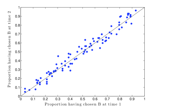
Figure 1: Proportion of decision makers having chosen option $B$ at time 2 as a function of the proportion of decision makers having chosen option $B$ at time 1 (there are 91 points, one for each of the 91 presented pairs of lotteries).

Stability over time of aggregate preferences is confirmed by the analysis of the most common choice, i.e. a lottery within each pair that is chosen by the majority of subjects. For this dataset, only for 4 out of 91 lottery pairs the most common choice shifted between time 1 and time 2. These lottery pairs are listed in Table 2. Notably, choice alternatives within each of these 4 pairs are characterized by relatively close expected values.

Table 2: The only 4 out of 91 pairs of lotteries, for which the most common (i.e. majority) choice has shifted between two repetitions of the experiment (time 1 and time 2). The choice is between lottery A and B. The most common choice at time 1 is highlighted in bold. Choice alternatives within each pair are characterized by relatively close expected values.

Lottery $A$					Lottery $B$					Expected value
$V_{1}^{A}$	$p_{1}^{A}$	$V_{2}^{A}$	$p_{2}^{A}$		$V_{1}^{B}$	$p_{1}^{B}$	$V_{2}^{B}$	$p_{2}^{B}$		Lottery $A$	Lottery $B$
56	0.05	72	0.95		68	0.95	95	0.05		71.2	69.35
88	0.29	78	0.71		53	0.29	91	0.71		80.9	79.98
-8	0.66	-95	0.34		-42	0.93	-30	0.07		-37.58	-41.16
96	0.61	-67	0.39		71	0.50	-26	0.50		32.43	22.5

Stability at the aggregate level is accompanied by variability of individual choices. In Figure 1, a significant scatter around the diagonal indicates a stochasticity in the revealed preferences of the decision makers. The individual deviation of choices between times 1 and 2 is further quantified in Figure 2, which plots the number of lottery pairs for which a given proportion of subjects has changed their choice. One can observe that individual choices of decision makers may vary significantly over time. In more than half of the binary lotteries, more than 30% of the subjects changed their answer between time 1 and time 2. The average rate of choice reversal (switching) per subject is slightly higher than 29%, which is in line with the values previously reported in the literature.

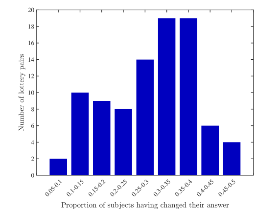
Figure 2: Histogram over all 91 lottery pairs of the proportion of decision makers having changed their choice between times 1 and 2. Note that the ordinate values of the ten bins sum up to 91. For more than half of the considered lottery pairs (48 out of 91), more than 30% of the subjects shifted their preference from $A$ to $B$ or vice-versa, between times 1 and 2.

3.2.2 Quantitative rationalisation via probabilistic choices

The combined observation of the overall stability of the choices at the aggregate level (Figure 1) and their variability at the individual level (Figure 2) adds to the large body of empirical literature discussed in the introduction that purports that decisions are probabilistic rather than deterministic. However, it is interesting to test it quantitatively as follows. For this, we propose a non-standard approach, which abstracts from any assumption on the probability model, algebraic core, and on the stimuli that promote the decisions. We straightforwardly derive the probability of a choice shift between times 1 and 2 from a single ingredient – the frequency of that choice observed at time 1 as a measure of the corresponding prospect probabilities, without any fit. In other words, the frequency of a given choice over the population of decision makers is taken as a probe for the underlying probability for that choice, used in the usual frequentist interpretation of probabilities [136].

Considering a given pair of lotteries, let us denote by $X_{t}$ the event “choosing lottery $X\in\{A,B\}$ at time $t\in\{1,2\}$”. For instance, if the decision maker chooses lottery $A$ at time 1 and lottery $B$ at time 2, this is represented by the combined event $A_{1}\bigcap B_{2}$. The overall stability of the choices at the aggregate level (figure 1) suggests the parsimonious assignment of a fixed stable probability $p_{j}$ for each of the two choices in a given lottery pair $j$:

$$\mathbb{P}\left(A_{1,j}\right)=\mathbb{P}\left(A_{2,j}\right)=p_{j}$$ (1)

and

$$\mathbb{P}\left(B_{1,j}\right)=\mathbb{P}\left(B_{2,j}\right)=1-p_{j}~{}.$$ (2)

This hypothesis consists in neglecting any heterogeneity between decision makers, thus assuming that they all have the same preference. Notwithstanding its simplicity, we now show that it is remarkably powerful at accounting for most of the observed shifts between times 1 and 2.

Indeed, because each choice among two lotteries within a pair is assumed probabilistic, this implies that repeating the experiment is expected to give possible choice shifts from $A$ to $B$ and vice-versa, just from the hypothesised probabilistic nature of the choice. Thus, the probability that a decision maker shifts her choice in a pair of lotteries is given by:

$$\mathbb{P}\left(\text{shift}\right)=\mathbb{P}\left(A_{1}\bigcap B_{2}\right)+\mathbb{P}\left(B_{1}\bigcap A_{2}\right)~{}.$$ (3)

This expression conveys the fact that the shift could occur from the choice $A$ at time 1 followed by the choice $B$ at time 2. This is represented by $A_{1}\bigcap B_{2}$. Or the decision maker might have chosen $B$ at time 1 followed by the choice $A$ at time 2. This is represented by $B_{1}\bigcap A_{2}$. Considering both scenarios together leads to expression (3).

The analysed experiment was conducted twice with the same decision makers, facing the same set of lottery pairs. Therefore, the successive decisions $A_{1}\bigcap B_{2}$ or $B_{1}\bigcap A_{2}$ are dependent because it is a repeated measure by design. However, let us assume that, when they form their choice at time 2, decision makers have forgotten their choices performed at time 1 (which is likely in the experimental set-up as the two iterations – time 1 and time 2 – were conducted approximately 2 weeks apart and the choice orders have been randomised). In the framework where their decisions are solely and completely captured by equations (1) and (2) expressing an intrinsic probabilistic choice structure, for a pair of lotteries we have $\mathbb{P}\left(A_{1}\bigcap B_{2}\right)=\mathbb{P}\left(B_{1}\bigcap A_{2}\right)=p(1-p)$, yielding

$$\mathbb{P}\left(\text{shift}\right)=2p\left(1-p\right)~{}.$$ (4)

This expression is the simplest and most parsimonious prediction for the probability $\mathbb{P}\left(\text{shift}\right)$ that a decision maker shifts her choice from time 1 to time 2. It is based on considering human behavior at the aggregate level, i.e., specifically that the fraction of persons making a given decision is equal (and equivalent) to the probability of a single random person to make that decision. This hypothesis is at the foundation of quantum decision theory and we refer to the Appendix and references therein for its motivation and justification. The second assumption underlying expression (4) is that decision makers have not kept the memory of their previous decision performed two weeks earlier. Given the neutral nature of the decisions (choosing between lotteries), this is likely to be a reasonable assumption. In the end, these assumptions made for simplicity have the virtue of leading to a prediction for $\mathbb{P}\left(\text{shift}\right)$ that is a function of a single variable $p$, which is itself measurable in the first experiment at time 1, leading to a parameter-free prediction.

In order to test the validity of prediction (4) on the experimental data, as mentioned above, we assume that the frequency of the most common choice for a given lottery pair over the ensemble of all decision makers (i.e. majority choice) is a proxy for the probability $p_{j}$.

Indeed, the frequency of the most common choice for a given pair $j$ of lotteries gives an estimate of the so-called frequentist definition of the corresponding probability [136], which converges to the true probability, if it exists, in the limit of very large samples. Similarly, we identify the probability $\mathbb{P}\left(\text{shift}\right)$ of a choice shift between times 1 and 2 with the proportion of decision makers having changed their choice between times 1 and 2.

This prediction (4), which has no adjustable parameters, is shown as the blue smoothed continuous curve in Figure 3, which plots the proportion of decision makers having changed their choice between times 1 and 2 as a function of the frequency of the most common choice at time 1.

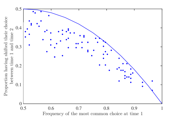
Figure 3: Proportion of decision makers having shifted their choice between time 1 and time 2 as a function of the proportion choosing the most frequently chosen option at time 1 (there are 91 points, each one represents a pair of lotteries). The solid line represents the proportion of shifts predicted by a simple model (4), assuming homogeneity of preferences, their stability at the aggregate level and choice independence between times 1 and 2. We stress that the solid line is not a “fit” as there are no adjustable parameters.

Figure 3 shows that the main dependence is rather well captured by prediction (4), which we stress again is not a “fit” as there is no adjustable parameter. Expression (4) has a simple intuitive interpretation: clear-cut choices associated with large $p_{j}$’s are aligned with strong and well-defined preferences, so that it is quite unlikely that a decision maker will change her choice; in contrast, when the frequency at time 1 for choosing a given lottery is close to even between the two lotteries, the decision makers are very likely to shift their choice at time 2. While these tendencies are obvious, what is less evident is the fact that the simple logical step leading to expression (4) accounts surprisingly well for the data, with no adjustment.

3.2.3 Evidence of heterogeneity between decision makers: a parsimonious description

While the agreement between data and prediction shown in Figure 3 is remarkable, given that the prediction has no adjustable parameters, it is also clear that the model over-estimates the number of decision shifts as the data tends to be systematically below the theoretical prediction, in particular for the pairs of lotteries with close ties, i.e. for which decision makers show a large heterogeneity of choices and the proportion choosing the most frequently chosen lottery is not much above 50%. More precisely, for more frequently chosen options (with frequency of the most common choice above 75%), the observed frequencies are closer to the theoretical prediction, while, for less frequently chosen options, the deviation is larger. This can explain the bimodal structure of the histogram in Figure 2.

In order to arrive at prediction (4), we have used two main assumptions:

(i) the choices between times 1 and 2 are made as if a single probability describes each of them (i.e. stability of the preferences and independence of choice between two repetitions of the experiment) and (ii) the decision makers’ preferences are homogenous, so that the same single probability $\{p_{j},\;j=1,...,91\}$ for each of the 91 pairs of lotteries characterises the full set of 142 subjects. We propose to keep the first assumption as part of a minimalist approach. As discussed briefly above, the second assumption flies in the face of enormous empirical evidence supporting the proposition that human decision makers exhibit significantly different risk preferences. This is particularly relevant to our discussion since the choices between the pairs of lotteries are specifically sensitive to the different levels of risk (as well as payoffs) associated with the competing lotteries in each pair.

Relaxing the assumption that all decision makers are identical can immediately be seen to help removing the discrepancy observed in Figure 3. Indeed, consider the simplest situation generalising heterogeneity, which consists in assuming the presence of two groups $i\in\left\{1,2\right\}$ of decision makers of size $142F$ and $142(1-F)$, respectively (with $0<F<1$), for which $P(A^{1}_{1,j})=P(A^{1}_{2,j})=p_{1,j}$ and $P(A^{2}_{1,j})=P(A^{2}_{2,j})=p_{2,j}$, where $A^{i}_{t,j}$ is the most frequent choice at time $t$ in a lottery pair $j$ by group $i$, and $p_{i,j}$ is a corresponding fixed probability of that choice for group $i$. Thus, for a given lottery pair the aggregate (over both groups) choice probability is

$$p=p_{1}F+p_{2}\left(1-F\right)~{}.$$ (5)

Then, the aggregate probability of shift for a given lottery pair is

$$\mathbb{P}\left(\text{shift}\right)=2Fp_{1}\left(1-p_{1}\right)+2(1-F)p_{2}\left(1-p_{2}\right)~{},$$ (6)

which is always smaller than its homogenised version (4). This results from the concavity of the function $f(p)=p(1-p)$. In the case $F=1/2$, this is also straightforwardly seen from the inequality $\left(p_{1}^{2}+p_{2}^{2}\right)/2\geq p_{1}p_{2}$. The equality between expression (6) and (4) with (5) is recovered obviously for the homogeneous case, i.e. for $F=0$ or $F=1$, or for $p_{1}=p_{2}$.

We now propose a simple quantitative model by assuming the following ansatz for $p_{1}$ and $p_{2}$:

$$\left\{\begin{aligned} p_{1}&=p+\alpha p\left(1-p\right)&\;\;\alpha\in\left[0,1\right]\\ p_{2}&=p-\beta p\left(1-p\right)&\;\;\beta=\alpha F/\left(1-F\right)\in\left[0,2\right]\end{aligned}\right.$$ (7)

where the value for $\beta$ derives from (5). Intuitively, the ansatz $p_{1}=p+\alpha p\left(1-p\right)$ in (7) states that the first group of decision makers tends to follow and overweight the majority choice when the two lotteries are difficult to tell apart (region of $p$ not too much larger than $1/2$). We can refer to this first group as “majoritarian”. The second ansatz $p_{2}=p-\beta p\left(1-p\right)$ in (7) states that the second group of decision makers tends to dislike the average preferred choice, the more difficult it is to decide between two lotteries. We call this second group “contrarian”.

Parameter $\alpha$ thus quantifies the difference between the majoritarians and contrarians in their tendencies to reproduce at time 2 their earlier choice at time 1. We do not claim that this parameterisation (7) is unique or has a strong theoretical basis. It is offered as a simple generalization, with one additional parameter, to the most parsimonious model (4). However, as Figures 4, 5 and 7 show, this simple ansatz provides an excellent fit to the data. We stress that the determination of the corresponding best $\alpha$ (and thus $\beta$) and $F$ is aided by the use of the bivariate Gaussian mixture model shown in Figure 4.

First, we compare this heterogeneous model (7) with the data by analysing decision makers with respect to their propensity to follow (or to oppose) the majority choice. For each decision maker, Figure 4 (left subplot) shows proportion of the most common (i.e. majority) choices in a choice set of a subject, observed during the two repetitions of the experiment (times 1 and 2). In other words, for each subject we plot the proportion of the lottery pairs, for which the choice of a subject coincides with the majority choice (at time 1 and 2). For this dataset, according to the likelihood ratio test (the Wilks test) [137], the hypothesis of a homogeneous population (a bivariate Gaussian model, $H_{0}$) is rejected with p-value $=1.4\times 10^{-7}$ in favor of a heterogeneous model (a bivariate Gaussian Mixture model, $H_{1}$). Probability density function of the latter is illustrated by the contour plot. The Gaussian mixture model has two components. The bigger (resp., smaller) component is characterized by a higher (resp., lower) proportion of the individual choices that coincide with the majority choice, with average value over times 1 and 2 equal to 0.76 (resp., 0.61). This feature of empirical clustering supports the suggested heterogeneous model (7) with two groups of decision makers: “majoritarian” (plus sign) and “contrarian” (circle).

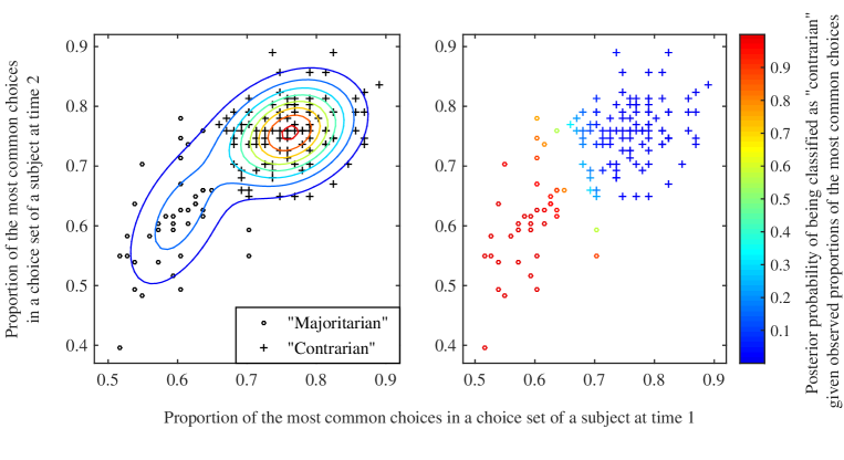
Figure 4: Proportion of the most common (i.e. majority) choices in a choice set of a subject, observed at two repetitions of the experiment (times 1 and 2). Each of the 142 data points represents one decision maker. The likelihood ratio (Wilks) test rejects the hypothesis of a homogeneous population ($H_{0}$: a bivariate Gaussian model) with p-value $=1.4\times 10^{-7}$ in favor of a heterogeneous model ($H_{1}$: a bivariate Gaussian Mixture model with 2 components). Probability density function of the latter is illustrated by the contour plot (left). The bigger (resp., smaller) component is characterized by a higher (resp., lower) proportion of the most common choices, with average value over times 1 and 2 equal to 0.76 (resp., 0.61). This empirical feature supports assumptions of the heterogeneous model (7) with two groups of decision makers: “majoritarian” (plus sign) and “contrarian” (circle). Right: Prevailing extreme values of posterior probabilities (either close to 1, or to 0 of the heat map) reflect low uncertainty of assessing an observed decision maker to a particular group: “majoritarian” (103 subjects $=73\%$) and “contrarian” (39 subjects $=27\%$).

For the same data, Figure 4 (right subplot) highlights posterior probabilities of a Gaussian mixture component (“contrarian”) given each observation. Prevailing extreme values of posterior probabilities (either close to 1, or to 0) reflect low uncertainty of assessing an observed decision maker to a particular group (i.e. unambiguous clustering), where 103 subjects ($73\%$) are classified as “majoritarian” and 39 subjects ($27\%$) – as “contrarian”.

Thus, the experimental data support the proposed classification of decision makers in two groups according to their propensity to follow (or to oppose) the most common choice (7), and the estimated size of the “majoritarian” group $F=0.73$.

At the second step, the model with heterogeneity (7) is calibrated to the same data as its homogeneous predecessor (4), which was shown in Figure 3. The starting values of parameters $\beta$ and $F$ are chosen with an iterated tabu search [138]. Recall that tabu search uses a local search procedure to iteratively move from one potential solution to an improved solution in the neighborhood of the starting point, until some stopping criterion has been satisfied. The term “iterated” refers to the fact that we start from many random initial conditions in the space of parameters.

Optimization results for the heterogeneous model are presented in Figure 5. This contour plot illustrates that the minimum residual sum of squares ($RSS_{min}=0.2331$) can be achieved by different combinations of the parameters $\beta$ and $F$. However taking into account the size of the “majoritarian” group that was estimated at the first step, i.e. $F=0.73$, the optimal value of $\beta=1.6$. Then, given (7), $\alpha=0.6$.

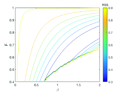
Figure 5: Contour plot of the residual sum of squares (RSS) obtained during calibration of the heterogeneous model (7). The starting values of parameters $\beta$ and $F$ are chosen with an iterated tabu search. The minimum $RSS_{min}=0.2331$ can be achieved by different combinations of the parameters. Given the estimated size of the “majoritarian” group, i.e. $F=0.73$ (Figure 4), the optimal value of $\beta=1.6$.

After its calibration, the model with heterogeneity (7) is expressed as

$$\left\{\begin{aligned} p_{1}&=p+0.6p\left(1-p\right)\\ p_{2}&=p-1.6p\left(1-p\right)~{},\end{aligned}\right.$$ (8)

which is represented in Figure 6. As intended, the decision makers referred to as “majoritarian” tend to follow the most common choice (average value of $p_{1}\approx 0.85$). In contrast, the decision makers that we call “contrarian” tend to weaken or even oppose the most common choice (average value of $p_{2}\approx 0.49$). Then, given equation (4), the average probability of shift for “majoritarian” group ($\approx 0.26$) in much lower, than for the “contrarian” group ($\approx 0.50$).

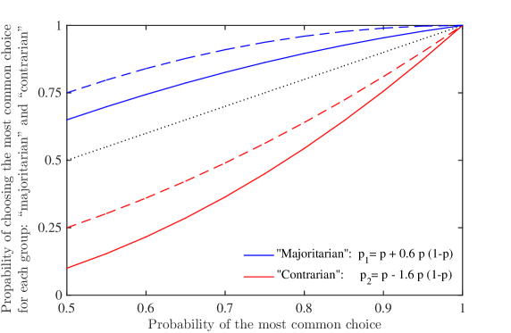
Figure 6: Probabilities $p_{1}$ and $p_{2}$ obtained by calibrating the heterogeneous model (7) with which the most common choice is chosen by each of the postulated two groups of decision makers as a function of the frequency $p$ of the majority choice aggregated over the whole population. The solid top (resp. bottom) curve shows $p_{1}$ (resp. $p_{2}$) of the “majoritarian” (resp. “contrarian”) decision makers, with the estimated size of the “majoritarian” group $F=0.73$. For reference: dotted line is the identity line ($y=x$); dashed lines represent the case of equal-sized groups ($F=0.5$ leading to the best estimates $\alpha=\beta=1$).

Finally, Figure 7 presents the same data as Figure 3 but now the model (7) is taking into account the heterogeneity of population, differentiating between the two groups of decision makers: “majoritarian” ($\approx 3/4$) and “contrarian” ($\approx 1/4$), with, respectively, $p_{1}$ and $p_{2}$ given by (8). The grey band represents the 90% confidence interval, which is delineated by the 5% and 95% quantiles, i.e. the area where 90% of the shifts should fall according to Monte Carlo simulations using the above model with two groups (3000 simulations per pair of lotteries). This allows us to quantify the uncertainty band resulting from sampling variabilities at times 1 and 2, using standard Bernouilli statistics. While this model is clearly over-simplified, it provides an excellent fit to the data confirming that, within the probabilistic choice framework, heterogeneity among decision makers is sufficient to account quantitatively for the observed changes of behaviour between repetitions of the experiment (times 1 and 2).

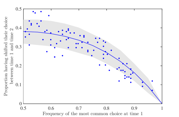
Figure 7: Same data as in Figure 3, which is compared with the prediction (6) of a heterogeneous population of two groups of decision makers with $p_{1}$ (“majoritarian”) and $p_{2}$ (“contrarian”) given by (8). The proportion of group sizes is approximately 3:1 in favor of “majoritarian”, i.e. estimated $F=0.73$. The shaded area represents the 5% and 95% quantiles, i.e. the area where 90% of the shifts should fall according to Monte Carlo simulations using the above heterogeneous model (3000 simulations per pair of lotteries).

4 Calibration of quantum decision theory

4.1 Brief presentation of stochastic cumulative prospect theory (logit-CPT) and quantum decision theory (QDT)

Based on the analysis of choice reversals in a repeated experiment, the previous section has shown that the hypothesis that decisions are probabilistic provides a parsimonious and quantitative description of decision making. We thus endeavour to test two probabilistic choice theories, (i) stochastic cumulative prospect theory (logit-CPT) and (ii) quantum decision theory. Both theories are summarised in the Appendix.

Here “quantum” model extends the “classical” CPT by including an attraction factor, which accounts for interfering choice options and a state of mind. These “quantum” interference effects explain with a single origin the observed systematic deviation from predictions of classical models. Nested models allow for straightforward quantitative comparison.

Prospect theory [20, 23] is now the most famous alternative to expected utility theory. The outcomes are quantified through a value function $v$, weighted by subjective probabilities obtained from the objective probability via a non-additive weighting function $w$. Moreover, the value function separates gains and losses, where the notions of gains and losses are defined with respect to a reference point, here assumed to be zero. Cumulative prospect theory (CPT) can be combined with a probabilistic choice function, allowing for probabilistic deviations from the option that maximises the choice criterion with respect to alternative options. There are many probabilistic extensions of CPT, some of which are modeling something entirely separate from response errors using polyhedral combinatorics, such as, e.g. in [107]. The probabilistic version of CPT that we use here is called logit-CPT because the probability weighting scheme uses the logit function (see Appendix and below). Such stochastic extension is often perceived as an add-on to an intrinsically deterministic CPT approach that is necessary to account for the observed stochasticity of human choices, interpreted as errors or unobserved components of an underlying deterministic process.

Quantum decision theory (QDT) is based on two essential ideas: (a) an intrinsic probabilistic nature of decision making and (b) a generalisation of probabilities using the mathematics of Hilbert spaces that naturally account for entanglement between choices [4, 42, 43, 48]. Thus, in contrast to logit-CPT, it places the probabilistic nature of choice at the center of its construction. As recalled in the Appendix (see expressions (35- 37)), a fundamental result of QDT is that the probability $p\left(\pi_{n}\right)$ of a given prospect $\pi_{n}$ can in general be decomposed as the sum of two terms according to

$$p\left(\pi_{n}\right)=f\left(\pi_{n}\right)+q\left(\pi_{n}\right)~{}.$$ (9)

The first term $f(\pi_{n})$ is associated with the utility of the prospect under consideration and, therefore, is called the utility factor. The second term $q(\pi_{n})$ accounts for interference and entanglement between prospect and state of mind, and results technically from the complex quantum nature of the probabilities describing the choices of decision makers. In decision theory, it characterizes subjective and subconscious processes of the decision maker related to other available prospects, as well as past experiences, beliefs and momentary influences, and is referred to as the attraction factor. We interpret the attraction factor as representing a subconscious attraction of a person to a given prospect. The attraction depends on the state of mind that can be influenced by external (i.e. situational) and/or internal (i.e. hunger, mood, fatigue, etc.) factors. For more precise definitions of the attraction factor, we refer to the Appendix and to [4, 42, 43, 48].

By the quantum-classical correspondence principle, when the quantum term $q(\pi_{n})$ becomes zero, the quantum probability reduces to the classical probability, so that $p(\pi_{n})\to f(\pi_{n})$ for $q(\pi_{n})\to 0$, with the normalization $\sum_{n}f(\pi_{n})=1$, with $0\leq f(\pi_{n})\leq 1$. In the sequel, we use a logit-CPT form for the utility factor $f(\pi_{n})$ given by expression (15) below, which corresponds to the first term in equation (16). We assume that logit-CPT can adequately characterize the utility of an isolated prospect for a decision maker. While logit-CPT incorporates some subjective deviations of values and probabilities, it treats each prospect separately, with no interference between the different prospects or no interference between a given prospect and the state of mind.

In QDT model, these interdependencies are incorporated via the attraction factor, which embodies the additional complex unconscious deliberations and preferences associated with decision making. By construction, it enjoys the following properties [4, 42, 43, 48]. It lies in the range $-1\leq q(\pi_{n})\leq 1$ and satisfies the alternation law $\sum_{n}q(\pi_{n})=0$. In addition, for a large class of distributions, there exists the quarter law

$$\frac{1}{N}\sum_{n=1}^{N}|q(\pi_{n})|=\frac{1}{4}\;.$$ (10)

In the presence of two competing prospects, one can show that, in the absence of any other information (the so-called “non-informative prior”), one obtains

$$|q(\pi_{n})|\approx 0.25~{},$$ (11)

which makes it possible to give quantitative predictions in absence of additional information [44, 45, 46, 47]. In the following, we go beyond (11) and introduce a mathematical expression (54) with constant absolute risk aversion (CARA) utility function (55) for the attraction factor, which corresponds to the second term in equation (20) and is motivated by the structure of the pairs of lotteries presented to the decision makers.

4.2 Methodology to estimate logit-CPT and QDT

We follow and extend the procedure of parameters estimation proposed by [57]. We first summarise their method and then extend it to QDT. Here, we use the same data set as studied in [57] to allow for a precise comparison and thus evaluation of the possible gains provided by quantum decision theory. The proposed QDT parameterization is obviously applicable to other data sets and we encourage readers to apply it to their own data sets.

According to stochastic decision theories, such as logit-CPT and QDT, the option $A_{j}$ of the pair $j$ of lotteries is chosen by a subject over the option $B_{j}$ with a probability $p_{A_{j}}$, which depends on individual parameters. These parameters can be estimated by fitting the model to the data obtained at time 1 and then used for predicting the outcomes at time 2.

The answers from the decision maker $i\in\left\{1\dots 142\right\}$ at time 1 are denoted $\left(\Phi_{j}^{i}\right)_{j=1}^{91}$:

$$\Phi_{j}^{i}=\left\{\begin{aligned} 0\text{ if subject $i$ chooses $A$ in the $j^{\text{th}}$ gamble},\\ 1\text{ if subject $i$ chooses $B$ in the $j^{\text{th}}$ gamble}.\end{aligned}\right.$$ (12)

Given the choices $\left(\Phi_{j}^{i}\right)_{j=1}^{91}$, the individual parameters of the decision maker $i$ can be estimated with a maximum likelihood method. A natural choice for the objective function is

$$\Pi^{i}=\prod_{j=1}^{91}p_{A_{j}}^{1-\Phi_{j}^{i}}p_{B_{j}}^{\Phi_{j}^{i}}~{}.$$ (13)

However, it has been shown [59] that this optimization method gives unreliable estimates at the individual level, since a shift of a single answer sometimes leads to very different parameters estimates. The hierarchical maximum likelihood method based on the work of [60] fixes this issue by introducing the assumption that the individual parameters are distributed in the population with a given density distribution. The optimization is then performed for each subject, weighting the objective functions with the density distributions obtained at the population level. In Ref. [57], this method has been applied to the experimental data described in section 3.1. Applied to stochastic CPT briefly described in the Appendix, the distributions of the parameters $\alpha$, $\lambda$, $\gamma$ and $\delta$ were assumed to be lognormal. Each log-normal distribution is defined through its location parameter $\mu$ and its scale parameter $\sigma$, which were estimated with a maximum likelihood method at the aggregate level.

The exactly same data and parameters estimation procedure were used in the analysis of the present article, which allows for a direct comparison of stochastic cumulative prospect theory and quantum decision theory. For stochastic cumulative prospect theory, we are able to recover precisely the quantitative results reported by [57]. In other words, we did not use the parameters reported by [57] but re-estimated them ourselves completely independently, reproducing entirely the whole calibration procedure for the logit-CPT. Then, we extended the procedure to calibrate and test QDT as explained below. The detailed description of the methodology follows.

$\bullet$ At the aggregate level

At the aggregate level, the parameters are estimated with a maximum likelihood method for both models (logit-CPT and QDT). The objective function is

$$\Pi^{\text{agg}}=\prod_{i=1}^{142}\prod_{j=1}^{91}p_{A_{j}}^{1-\Phi_{j}^{i}}p_{B_{j}}^{\Phi_{j}^{i}}~{},$$ (14)

where the probability of choosing option $A$ over option $B$ is defined as follows (see Appendix):

• – for logit-CPT:

  $$p_{A_{j}}=\frac{1}{1+e^{\varphi\left(\tilde{U}_{B_{j}}-\tilde{U}_{A_{j}}\right)}}~{},$$ (15)

• – for QDT:

  $$p_{A_{j}}=\frac{1}{1+e^{\varphi\left(\tilde{U}_{B_{j}}-\tilde{U}_{A_{j}}\right)}}+\min\left(f_{A_{j}},1-f_{A_{j}}\right)\tanh\left(a\left(U_{A_{j}}-U_{B_{j}}\right)\right)~{}.$$ (16)

To be clear, associated with the utility factor, ${\tilde{U}}$ represents the utility according to the CPT framework defined by expression (48), while $U$, which is defined by expression (55) as the CARA function with a coefficient of absolute risk aversion $\eta$, enters into the definition (54) of the attraction factor.

Note that the QDT formulation has two additional parameters ($a$ and $\eta$) compared to logit-CPT, so that the later is nested in QDT (it is retrieved from the QDT formulation by setting $a=0$).

$\bullet$ At the individual level

When applied finally to the individual level, the parameters are estimated with a hierarchical maximum likelihood method for both models (logit-CPT and QDT). In a nutshell, this means first estimating the distribution of parameters at the aggregate level to obtain prior distributions, which are then used as weights penalising possible over-determinations at the individual level. The objective function for each subject $i$ is

$$\Pi^{i}=g_{\alpha}g_{\lambda}g_{\gamma}g_{\delta}\prod_{j=0}^{91}p_{A_{j}}^{1-\Phi_{j}^{i}}p_{B_{j}}^{\Phi_{j}^{i}}~{},$$ (17)

where $g_{X}$ is the distribution of the parameter $X\in\{\alpha,\lambda,\gamma,\delta\}$, according to the experimental results from [57]. The probability of choosing option A over option B is defined as follows:

• – for logit-CPT identically as for the aggregate level in (15):

  $$p_{A_{j}}=\frac{1}{1+e^{\varphi\left(\tilde{U}_{B_{j}}-\tilde{U}_{A_{j}}\right)}}~{},$$ (18)

• – for QDT:

  $$p_{A_{j}}=\frac{1}{1+e^{\varphi(\tilde{U}_{B_{j}}-\tilde{U}_{A_{j}})}}+\min\left(f_{A_{j}},1-f_{A_{j}}\right)\tanh\left(a^{\text{agg}}\left(U_{A_{j}}^{\text{agg}}-U_{B_{j}}^{\text{agg}}\right)\right),$$ (19)

  $$p_{A_{j}}=\frac{1}{1+e^{\varphi\left(\tilde{U}_{B_{j}}-\tilde{U}_{A_{j}}\right)}}+\min\left(f_{A_{j}},1-f_{A_{j}}\right)\tanh\left(a\left(U_{A_{j}}-U_{B_{j}}\right)\right)~{},$$ (20)

  where the exponent “agg” indicates that, at the individual level, $a$ and $\eta$ are not seen as parameters, but replaced by their optimal values found at the aggregate level.

In particular, at the individual level, the QDT formulation involves the same number of individual parameters as the logit-CPT formulation.

The solver used for all the optimizations is the fminsearch function from MATLAB (Nelder & Mead simplex algorithm), the starting values of the parameters are chosen with a tabu search.

4.3 Calibration and prediction at the aggregate level

At the aggregate level, the optimization problem for QDT involves seven parameters: five for the QDT utility factor, equation (51), which is identical to the logit-CPT formulation, and two original parameters for the QDT attraction factor, equation (54). Thus, the logit-CPT model is nested in the QDT one (null hypothesis: $a^{\text{agg}}=0$) [56]. This implies that one has to be very careful with choosing a statistical test, so that it can “punish” the more general formulation (i.e., the unrestricted QDT model). Widely used methods of a relative quality estimation for the models with different number of parameters include Akaike information criterion (AIC) and Bayesian information criterion (BIC). Both criteria compare models’ goodness of fit, which is assessed by the likelihood function, while penalising for a larger number of estimated parameters. However for nested hypothesis, the AIC and BIC are superseded by the likelihood ratio test, which is in fact the most powerful test among competitors. We apply the log-likelihood ratio test (the Wilks test) to compare QDT and logit-CPT models. For nested hypotheses, one can show that two times the log-likelihood ratio has a chi-square distribution with a number of degrees of freedom equal to the difference in the number of parameters between QDT and logit-CPT (which is $2$, $a$ (16) and $\eta$ (55)), under the null that the generating process is the logit-CPT (i.e., the restricted model with the smaller number of parameters).

Performing the log-likelihood ratio test, we find that the null hypothesis (logit-CPT) is rejected at the 95% level. In other words, the logit-CPT model is insufficient to describe the data, and the QDT formulation with the novel attraction factor provides a significant improvement, which is sufficiently large to compensate for the “cost” of two additional parameters.

For the two models, the values of the parameters estimated at the aggregate level for all participants (i.e. with the assumption of homogeneity) are highlighted in bold in Table 3. For the QDT attraction factor $q$, the CARA utility function $U$ with the obtained parameter $\eta=0.05$ is illustrated in Figure 8. In particular, since $|q|$ depends on the utility difference $U_{A}-U_{B}$ of the alternative lottery options $A$ and $B$, the attraction factor is small except for some gambles involving big losses. Thus, the QDT attraction factor accounts for the experimental observation that decision makers do not care much about medium payments, but respond to large losses. Note that the typical size of the CARA coefficient $\eta$ is set by the size of the initial wealth and of the payoffs of the lotteries.

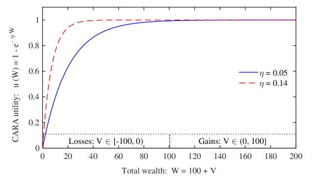
Figure 8: Constant absolute risk aversion (CARA) utility function. In the experiment, the outcomes $V$ of choice options (i.e. binary lotteries defined in table 1) are between $-100$ and $100$, and the initial endowment $W_{0}=100$, thus, the total wealth $W\in[0,200]$. With this utility function and expression (54), with $\eta=0.05$ (for the majority of decision makers) the attraction factor $q$ is small except for pairs of lotteries involving big losses. Higher value of $\eta=0.14$ (for “contrarian” group) reduces this $q$ effect to a narrow range of extreme losses.

Most of the parameters describing the QDT utility term ($\alpha$, $\gamma$, $\delta$ and $\varphi$) are close to those obtained with logit-CPT. However, for QDT the loss aversion parameter $\lambda$ is smaller. This means that within QDT, though losses loom larger than gains in general ($\lambda>1$), a part of this effect, namely, aversion to big losses, is transferred to the QDT attraction factor ($q\neq 0$).

Table 3: Estimated at the aggregate level, parameters of logit-CPT and QDT. For ALL decision makers (in bold), values of $\alpha,\delta,\gamma,\varphi$ parameters are close for both models. The loss aversion parameter $\lambda$ is smaller with QDT (though $>1$) because aversion to large losses is transferred to the QDT attraction factor ($a$ (16) and $\eta$ (55)). Heterogeneity is introduced by classifying decision makers into “majoritarian” ($\approx 3/4$) and “contrarian” ($\approx 1/4$) based on their propensity to follow/oppose the majority choice (model (7), Figure 4). For “majoritarian” group, the QDT attraction factor (i.e. aversion to big losses) is even more acute, increasing the relevance of QDT. In contrast, for “contrarian” group, the QDT attraction factor has less impact due to the decrease in $a$, bringing closer predictions of both models.

	Decision makers:	$\alpha^{\text{agg}}$	$\lambda^{\text{agg}}$	$\delta^{\text{agg}}$	$\gamma^{\text{agg}}$	$\varphi^{\text{agg}}$	$a^{\text{agg}}$	$\eta^{\text{agg}}$
logit-CPT	ALL,	0.73	1.11	0.88	0.65	0.30	-	-
	including:
	“majoritarian”	0.72	1.13	0.91	0.69	0.41	-	-
	“contrarian”	0.86	0.98	0.78	0.40	0.08	-	-
QDT	ALL,	0.69	1.02	0.89	0.63	0.37	1.47	0.05
	including:
	“majoritarian”	0.68	1.03	0.92	0.66	0.50	2.07	0.05
	“contrarian”	0.80	0.93	0.77	0.40	0.11	0.61	0.14

Figure 9 (main plot) demonstrates performance of the two models regarding the types of lotteries. For each pair of gambles, absolute residuals of the choice frequencies, i.e. distances between their estimated values and those observed at the first iteration of the experiment (time $1$), are compared. For the QDT model absolute residuals are smaller, in particular, for mixed and pure loss lotteries that involve big losses. Though, for other lotteries, the improvement might not seem significant, table 4 shows that QDT reduces the residual sum of squares (RSS) when summed over all gambles, as well as separately over each type of gambles: pure loss, pure gain and mixed lotteries. In other words, due to the fact that QDT discriminates between high aversion to big losses and only moderate aversion to small losses, QDT outperforms logit-CPT for all types of lotteries.

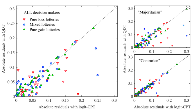
Figure 9: Left main plot: Distances between choice frequencies estimated at the aggregate level (with logit-CPT and QDT) and those observed at the first iteration of the experiment (time 1). Each of the 91 points is a pair of lotteries of a certain type: pure loss (red downward triangles), pure gain (green upward triangles) and mixed lotteries (blue circles). The QDT model (y-axis) performs better than logit-CPT (x-axis) for gambles appearing in the lower triangle below the diagonal. Right subplots: The same values calculated for the two groups of decision makers: “majoritarian” and “contrarian”. The main improvements are achieved with QDT for mixed and pure loss lotteries, which involve big losses, and mostly within the “majoritarian” group.

Table 4: For lottery types, at the aggregate level, statistics of the fit (time 1) and prediction (time 2) for both parametrisations – logit-CPT and QDT. The QDT model outperforms in both iterations of the experiment: (i) the residual sum of squares (RSS) is smaller when calculated for All lottery pairs, as well as separately for each type – pure loss/gain and mixed lotteries; (ii) the correlation is closer to 1.

Residual sum of squares (RSS) for:		logit-CPT	QDT
ALL types of lotteries,	FIT (time 1)	0.73	0.52
	PREDICTION (time 2)	0.76	0.59
including:
pure loss lotteries	FIT (time 1)	0.22	0.15
	PREDICTION (time 2)	0.26	0.13
mixed lotteries	FIT (time 1)	0.27	0.17
	PREDICTION (time 2)	0.21	0.18
pure gain lotteries	FIT (time 1)	0.24	0.21
	PREDICTION (time 2)	0.29	0.28
Correlation	FIT (time 1)	0.93	0.95
	PREDICTION (time 2)	0.93	0.95

4.4 Calibration and prediction at the aggregate level for two groups of decision makers

Section 3.2.3 demonstrated that experimentally observed choice reversals can be to a large degree explained by a simple probabilistic model, when heterogeneity of population is introduced. Decision makers were differentiated into two groups – “majoritarian” and “contrarian” in proportion $\approx 3:1$, – based on their propensity to follow/oppose the majority choice (model (7), Figure 4). In the current Section, parameters of the two models — logit-CPT and QDT – are calibrated for each group separately.

Table 5 compares the obtained residual sum of squares (RSS) of the fit (time 1) and prediction (time 2) for both models. The RSS is consistently lower with the QDT model for all decision makers, as well as for each group. At the same time, introducing heterogeneity slightly increases the RSS in comparison with the assumption of homogenous population, especially for predictions, which may indicate overfitting. The only improvement in the RSS is observed for the fit of “contrarian” group with logit-CPT, so that for this group results of both models become quite close to each other.

Table 5: Accounting for heterogeneity, at the aggregate level, the residual sum of squares (RSS) of the fit (time 1) and prediction (time 2) for both parametrisations – logit-CPT and QDT. For both groups, the RSS is consistently lower with QDT than with logit-CPT. However, the RSS slightly increases in comparison with the assumption of homogenous population (All decision makers), especially for the prediction, which indicates overfitting. The only improvement of the RSS is observed for the fit of “contrarian” group with logit-CPT, so that for this group results of both models become close to each other.

Residual sum of squares (RSS) for:		logit-CPT	QDT
ALL decision makers,	FIT (time 1)	0.73	0.52
	PREDICTION (time 2)	0.76	0.59
including:
“majoritarian”	FIT (time 1)	0.96	0.66
	PREDICTION (time 2)	1.03	0.78
“contrarian”	FIT (time 1)	0.59	0.53
	PREDICTION (time 2)	1.04	0.97

Parameters of the logit-CPT and QDT models, estimated at the aggregate level for each group are presented in Table 3. Within both models, classification of participants into two groups affected the estimates of the parameter $\varphi$, i.e. steepness of the logit choice function (51). “Majoritarian” decision makers have the highest $\varphi$ that reveals a higher degree of conviction in their own choice. This finding is in agreement with the heterogeneous shift model (7) and Figure 6, which predict a lower probability of choice shift between repetitions of the experiment for “majoritarian” group (Section 3.2.3). For the “contrarian” participants, the low value of $\varphi$ is in line with the prediction of a larger probability of the choice shift.

Within QDT model, the most noticeable distinction between the two groups concerns the attraction factor $q$, which captures aversion to large losses. For “majoritarian” group, the QDT attraction factor is even more acute, than in the case of a homogenous population. Specifically, “majoritarians” are susceptible to losses of the same magnitude (the same $\eta$ (55)), but are more sensitive to them (larger $a$). In contrast, for “contrarian” group, the QDT attraction factor has small impact. Higher value of $\eta=0.14$ reduces the range of losses, to which participants are susceptible: “contrarians” are averse only to extreme losses, Figure 8. Moreover, they are less sensitive due to the decrease in parameter $a$. The small impact of the QDT $q$ factor on the “contrarian” group explains close predictive power of logit-CPT and QDT models.

This distinction between the groups becomes evident on the Figure 9 (right subplots). QDT visibly improves the fit for the “majoritarian” group in mixed and pure loss lotteries with big losses, due to the larger attraction factor. At the same time, “contrarian” decision makers are modeled similarly by both models.

4.5 Calibration and prediction at the individual level

At the individual level, since the two formulations include the same number of parameters, the model selection can be done according to the (log-)likelihoods: the preferred model is the one that has the largest (log-)likelihood. In other words, due to the same number of parameters, the Bayesian information criterion (BIC) and the Akaike information criterion (AIC) are redundant and equivalent to the direct comparison of the (log-)likelihoods. According to this criterion, we find that the QDT model has the highest predictive power: average, over decision makers, log-likelihood for this model is larger (table 6). Figure 10 provides a comparison of the individual log-likelihoods obtained with logit-CPT and QDT for each subject. The figure demonstrates better performance of the QDT model both for the fit (at time 1) and for the prediction (at time 2).

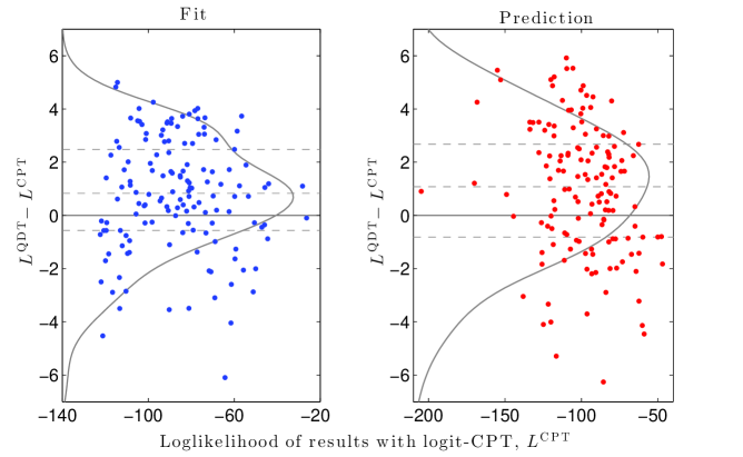
Figure 10: Difference of log-likelihoods (y-axis, QDT minus logit-CPT) as a function of the log-likelihoods obtained with logit-CPT (x-axis). There are 142 points in each plot, each point represents a decision maker. QDT performs better for points with positive y-coordinate (i.e. when QDT leads to a larger log-likelihood). The left plot shows the results of the fit (time 1), and the right plot shows the results of the prediction (time 2). For both plots, the solid curves represent the kernel estimated density of the difference of log-likelihoods, and the dashed lines their median and quartiles.

Table 6: Model selection based on the calibration at the individual level. Average over decision makers log-likelihood is larger for QDT, thus according to this criterion the QDT model is preferred to logit-CPT. Since the two models have the same number of parameters, the AIC and BIC criteria produce the same result. Average fractions of choices in a choice set of a subject explained (at time 1) and predicted (at time 2) are also larger for the QDT model.

Average over decision makers:		logit-CPT	QDT
individual log-likelihood:	FIT (time 1)	-86.53	-85.77
	PREDICTION (time 2)	-99.31	-98.34
explained (predicted) fraction of choices:	FIT (time 1)	0.76	0.77
	PREDICTION (time 2)	0.73	0.74

The QDT model is also selected according to the explained fraction of choices in a choice set of a subject. At both iterations of the experiment – time 1 (fit) and time 2 (prediction) – the average explained (predicted) fraction of choices is slightly larger for QDT, than for logit-CPT (table 6).

Figure 11 summarizes model selection on the individual basis. According to the (log-)likelihood criterion, QDT strictly outperforms logit-CPT for $2/3$ of decision makers. When comparing the explained (predicted) fraction of choices, the QDT model performs better for a half of subjects and at least as good as logit-CPT for another 20% of participants. Thus, for both criteria the logit-CPT model has superior performance only for one third of the individuals.

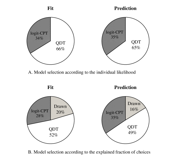
Figure 11: On the individual basis, model selection – QDT (white), logit-CPT (dark grey) or drawn among models (i.e. equal results, light grey) – at two repetitions of the experiment: time 1 (fit, left) and time 2 (prediction, right). Upper: According to the individual (log-)likelihood criterion, QDT strictly outperforms logit-CPT for $2/3$ of decision makers. Lower: According to the individual explained (predicted) fraction of choices, the QDT model performs better for a half of subjects and at least as good as logit-CPT for another 20% of participants. Thus, for both criteria the logit-CPT model has superior performance only for $1/3$ of the individuals.

A closer look at the predicted fractions of choices for each pair $j$ of lotteries (Figure 12) reveals that the improvement obtained with QDT is especially noticeable in some gambles including big losses. For those particular gambles, the quantum attraction factor is very significant. For the other gambles, the predictions are of the same quality with both methods. Indeed, the individual parameters obtained for the QDT utility factor tend to differ by less than 10% from those obtained with logit-CPT (see Figure 13): this implies that, for lotteries with negligible attraction, QDT gives individual predictions that are close to those given by logit-CPT.

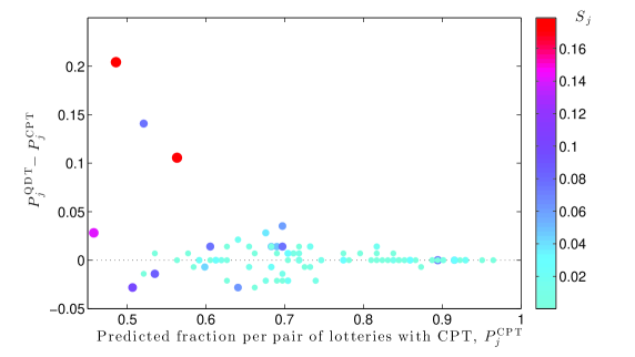
Figure 12: $P_{j}^{\text{QDT}}$ (resp. $P_{j}^{\text{CPT}}$) represents the fraction of choices correctly predicted for the pair $j$ of lotteries with QDT (resp. logit-CPT). The difference between the two predicted fractions is plotted against the predicted fraction obtained with logit-CPT. For points in the upper part of the plot above the dotted line, QDT preforms better. The colors and sizes of markers encode the average intensity of the attraction factor among $N=142$ subjects: $S_{j}=\frac{1}{N}\sum_{i=1}^{N}|q_{A_{j}}^{i}|$.

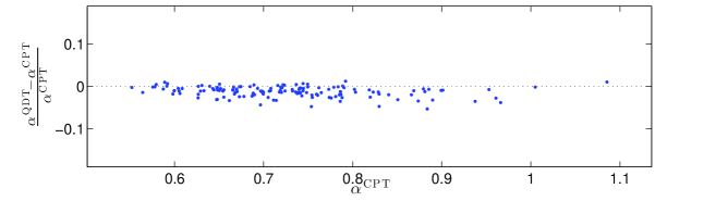
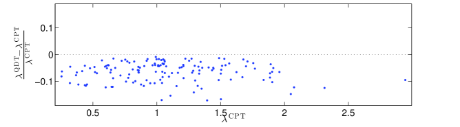
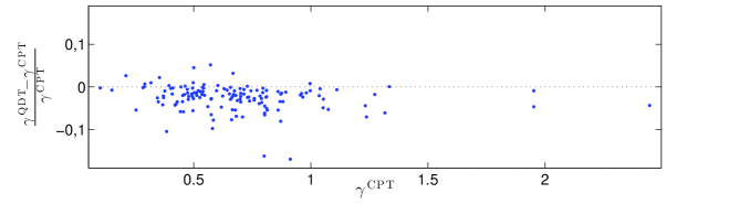
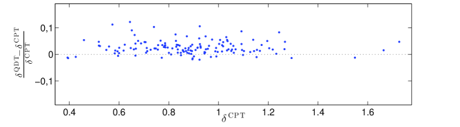
Figure 13: Relative difference of parameters estimates (QDT minus logit-CPT) against estimates obtained with logit-CPT. Though for all parameters and most subjects the absolute relative difference are smaller than 10%, some trends are noticeable. In particular, in the presence of a quantum factor for extreme losses, the loss aversion $\lambda$ tends to be smaller than with logit-CPT.

In conclusion, at both aggregate and individual levels, the QDT model, with the attraction factor that captures aversion to large losses, outperforms the logit-CPT model according to a number of criteria. While the improvements of these diagnostics obtained with QDT over logit-CPT are not large, they are of the same size as those obtained by [57] in their evaluation of different competing models (excluding QDT). In section 5, we propose an explanation for these results, i.e. difficulty in considerable improvement of choice prediction, based on an intrinsic limit of predictability associated with the intrinsic probabilistic nature of decision making.

5 Limits of predictability with probabilistic choices

We return to the considerations and tests of Section 3 that strongly suggest that decisions are probabilistic rather than deterministic. We test further this hypothesis and show that it allows us to quantitatively account for the limits of predictability observed in the experiments.

Indeed, Table 6 and Figures 10-11 show that the current analytical formulation of QDT allowed us to improve the individual fit and prediction for most subjects and on average, but with a rather small improvement of prediction on average, going from 73% for logit-CPT to $74\%$ for QDT. The same issue was encountered by [57] who found that, while their implementation of the hierarchical maximum likelihood method improved the reliability of the parameter estimates and the log-likelihoods of results at time 2, the average predicted fraction did not improve compared with the one obtained with the usual maximum likelihood estimation method. This hints at a hard “barrier” preventing to improve further the fraction of decisions. Actually, if choices are probabilistic, this barrier obtains a natural explanation.

5.1 Distribution of the predicted fractions

For a given pair of lotteries $j\in\{1\dots N\}$ and a given decision maker $i$, we define the probability $p^{i}_{A_{j}}$ with which the lottery $A$ is picked over $B$. Likewise, a probability $p^{i}_{B_{j}}$ is defined, and $p^{i}_{B_{j}}=1-p^{i}_{A_{j}}$.

Suppose that the probabilities $p^{i}_{A_{j}}$ and $p^{i}_{B_{j}}$ are known and stable in time. Then the best prediction for the pair of lotteries $j$ is to assume that the decision maker will prefer the most likely choice. Consequently, the choice regarding lotteries of the pair $j$ can be seen as a Bernoulli trial, with a probability of success $p^{i}_{j}$ larger than 0.5:

$$p^{i}_{j}=\max\left(p^{i}_{A_{j}},p^{i}_{B_{j}}\right)$$ (21)

Let $P^{i}$ be the fraction of choices predicted correctly for subject $i$. $P^{i}$ corresponds to the fraction of successes in a sequence of $N$ independent Bernoulli trials with different probabilities of success. Thus the random variable $P^{i}$ follows a Poisson binomial distribution.

Given the success probabilities $\left(p^{i}_{j}\right)_{j\in\{1\dots N\}}$, the discrete distribution can be numerically approximated using a discrete Fourier transform [61] by the following formula:

$$\left\{\begin{aligned} &\mathbb{P}\left(P^{i}=k/N\right)=\frac{1}{N+1}\sum_{l=0}^{N}C^{-lk}\prod_{m=1}^{N}\left(1+\left(C^{l}-1\right)p^{i}_{j}\right)&\;\;\;k\in\left\{0\dots N\right\}\\ &C=\exp\left(\frac{2\omega\pi}{N+1}\right)&\end{aligned}\right.$$ (22)

where $\omega$ stands for the pure imaginary number such that $\omega^{2}=-1$.

For the experiment described in Section 3.1, the theoretical Poisson binomial distributions of the predicted fraction of choices for a group of typical decision makers are plotted in Figure 14. For these distributions, individual prospect probabilities of the most likely choice ($p^{i}_{j}>0.5$) for each of the 91 pairs of lotteries $j$ are estimated with the QDT model at time $1$. These values are then inserted in expression (22) to explain (“in-sample) at time $1$ and predict (“out-of-sample”) at time $2$ the fraction of correct choices (“correct” in the sense that the choice corresponds to the probability larger than $0.5$ as estimated by the QDT calibration). The group of typical decision makers (7 subjects) is chosen such that the mode of their theoretical Poisson binomial distribution $P^{i}$ is equal to 0.77, i.e. the median value among the population (see Figure 11, inserted plot). For this group of typical decision makers, the theoretical probability to predict more than 85% of the answers is 2.8%. Similarly to the subjects whose distributions are shown in Figure 14, for most decision makers in the experiment, we found prospect probabilities for which it was very unlikely to predict more than 85% of the answers. Figure 15 presents the frequencies, among all 142 subjects, of the probability of the theoretical predicted fraction of choices $P^{i}$ to be larger than 85%. From this figure, we can extract the following representative statistics: for 56% of the population (80 subjects), the theoretical probability to predict correctly more than 85% of the choices (i.e. $P^{i}>85\%$) is less than 5%; for 42% of the decision makers (60 subjects), the probability of $P^{i}>85\%$ is less than 1%; for 28% (40 subjects), it is less than 0.1%. Consequently, even if the decision maker’s preferences are stable and if the estimated probabilities are very accurate, the probabilistic nature of the approach does not allow one to improve the choice predictions beyond its theoretical limit (which remains randomly distributed).

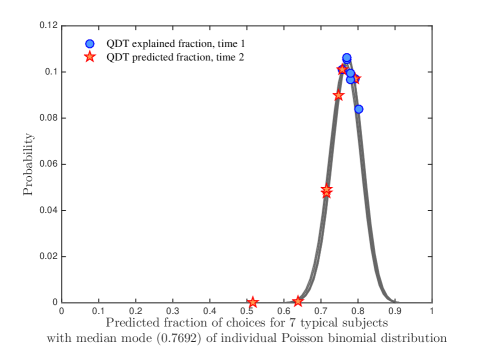
Figure 14: Theoretical Poisson binomial distributions of the predicted fraction of choices, $P^{i}$, of a group of 7 typical (with their mode of $P^{i}$ equal to 0.77, i.e. median value within the population: see Figure 15, inset). For these theoretical distributions, individual prospect probabilities of the most likely choice ($p^{i}_{j}>0.5$) for each of the 91 pairs of lotteries $j$’s are estimated within the QDT model at time $1$. The observed fractions of choices (i) explained at time $1$ i.e. “in-sample” (blue circles) and (ii) predicted for time $2$ i.e. “out-of-sample (red pentagram) with the QDT model, are indicated on the plot. For this group of typical decision makers, the theoretical probability to predict more than 85% of the answers is 2.8%.

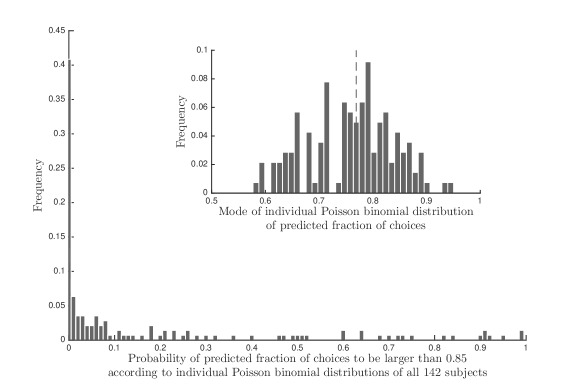
Figure 15: Main plot: Frequencies, over all 142 subjects, of the probability of the theoretical predicted fraction of choices $P^{i}$ to be larger than 85%. For 56% of the population (80 subjects), the theoretical probability to predict more than 85% of choices is less than 5%. Inset: Frequencies, over all 142 subjects, of the modes of theoretical individual Poisson binomial distributions of the predicted fraction of choices, with median value representing a “typical” decision maker indicated by dashed line.

5.2 Distribution of predicted fractions at the aggregate level

Since only one predicted fraction at time $2$ is observed for each subject, it is not possible to verify at the individual level whether the predicted fraction $P^{i}$ of choices really follows the Poisson binomial distribution described in the previous subsection. However, assuming that the subjects belong to a homogeneous population (as discussed in sections 3.2.3 and 6, this assumption is not perfect but is useful as a first-order approximation), it is possible to approximate the distribution of the predicted fraction throughout the population, and to compare it to the histogram of the 142 observed predicted fractions at time $2$.

For this purpose, we now consider that the Poisson binomial distribution of the fraction $P^{i}$ of choices predicted correctly for subject $i$ can be approached with the classical binomial distribution $\mathcal{B}\left(p^{i},N\right)$, where $p^{i}$ is defined by (see Figure 16, left panel):

$$p^{i}=\frac{1}{91}\left\lfloor\sum_{j=1}^{91}p^{i}_{j}\right\rfloor\in\left\{\frac{45}{91},\frac{47}{91}\dots\frac{91}{91}\right\}\;.$$ (23)

Moreover, we assume that the probability to pick a subject such that $P^{i}\sim\mathcal{B}\left(k/N,N\right)$, with $k\in\left\{45,\dots 91\right\}$, is equal to the frequency with which $p^{i}=k/N$ (Figure 16, right panel). For each subject, this observed average prospect probability $p^{i}$ of the most likely choice ($p^{i}_{j}>0.5$) among 91 pairs of lotteries is estimated at time $1$ with the QDT model. These approximations provide accurate representations of the results.

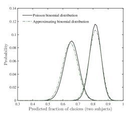
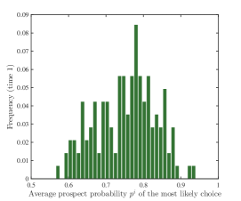
Figure 16: Left: Theoretical Poisson binomial distributions (black solid line) of the predicted fractions of choices for two distinct subjects as described in subsection 5.1, and their approximating binomial distributions (green dash-dotted line). Right: Histogram, over 142 subjects, of their observed average prospect probabilities $p^{i}$ of the most likely choice ($p^{i}_{j}>0.5$) among 91 pairs of lotteries, estimated at time $1$ with the QDT model (for each subject, $p_{i}$ also corresponds to the mean of her theoretical predicted fraction of choices distributed according to the Poisson binomial law, and the approximating binomial law).

The theoretical distribution of the predicted fraction of choices throughout the population (142 subjects) is estimated by approximating binomial distributions, with success probabilities in the interval $(0.5;1]$, which are then weighted by the observed frequencies of the average prospect probabilities $p^{i}$ (see Figure 17). Assuming that the prospect probabilities, estimated at time 1, are accurate and stable in time and can thus be used at time 2 (to perform an “out-of-sample” prediction), the obtained theoretical distribution of the predicted fraction of choices in the population is given by the black solid line in Figure 18. The red histogram corresponds to the predicted fractions observed at time 2. The approximated theoretical distribution for the predicted fraction appears to be close to the experimental one. In particular, both are skewed to the left: this suggests that bad predictions at the individual level may follow inevitably from the probabilistic nature of the choice.

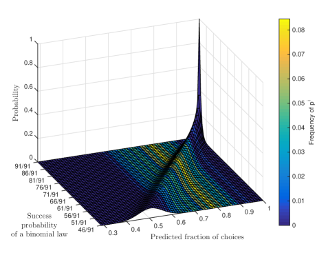
Figure 17: Estimation of a theoretical distribution of the predicted fraction of choices throughout the population (142 subjects), which is obtained by combining the approximating binomial distributions, with success probabilities in the interval $[46/91;91/91]$, with weights determined by the observed frequencies of the average prospect probabilities $p^{i}$ of the most likely choice at time $1$ with QDT model (see Figure 18).

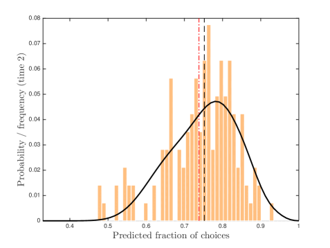
Figure 18: Approximated theoretical distribution (black solid line) of the predicted fraction of choices throughout the population (142 subjects). The histogram represents the fractions of choices correctly predicted “out-of-sample” at time $2$ with QDT estimated at time $1$. Mean values are indicated by the black dashed line for the theoretical distribution and by the red dash-dotted line for the experimental distribution. These values are reported in Table 7.

Table 7: Estimated and experimental moments of the predicted fractions throughout the population.

	Approximated distribution	Experimental distribution
Mean	0.75	0.74
Standard deviation	-0.09	-0.09
Skewness	-0.3	-0.8

Performing the Kolmogorov-Smirnov test to compare the theoretical and observed distributions of predicted fraction shown in Figure 18, we fail to reject at the 5% significance level the null hypothesis that the experimental distribution of the predicted fraction is generated by the theoretical one: the p-value is 0.254, and the value of the test statistic is 0.08 (corresponding to the maximum distance shown by the arrow in Figure 19.

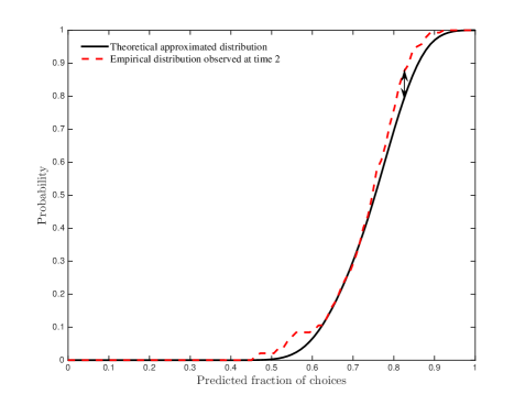
Figure 19: Theoretical (black solid line) and experimental (red dashed line) cumulative distribution functions (CDF) of the predicted fractions of choices over the population (142 subjects). The arrow shows the maximum distance between the two curves (value of the test statistic for the Kolmogorov-Smirnov test equal to 0.08).

Table 7 and Figure 19 compare the estimated cumulative distribution function (CDF) of the predicted fraction and the experimental one. Though the Kolmogorov-Smirnov test fails to reject the null hypothesis as just mentioned, this figure highlights a difference between the two CDF: the theoretical CDF seems to almost dominate stochastically the experimental one, i.e., the predicted fractions are less good than expected. The reason may be that the model is slightly overfitting. In other words, if a subject picks lottery $A$ with probability $p_{A}>0.5$, and actually chooses $A$ at time 1, then maximising the likelihood might lead to overestimating $p_{A}$, thereby overestimating the “probability of success” when making the prediction that the subject will choose $A$ at time 2.

6 Further remarks on the link between the probabilistic shift model and QDT

Analysis of the probabilistic shift model in Sections 3.2.2 and 3.2.3 was focused on the majority choice. We chose to approximate the theoretical probability $p$ in equation (4) for homogenous population, and $p_{1}$ and $p_{2}$ in equations (5)-(7) with heterogeneity, by an observed frequency of the most common choice for a given lottery pair over decision makers. Naturally, empirical clustering of the participants of the experiment (Figure 4) was based on the same criterion – their tendency to follow/oppose the majority choice. As a consequence, the sign and value of the estimated parameters $\alpha$ and $\beta$, equation (8), characterize the two groups only with respect to their (dis-)agreement with the majority. In order to make further inferences about risk attitudes, they should be estimated within additional models. In particular, our QDT model identified higher susceptibility of the “majoritarian” group towards big losses.

However, it is important to notice that the probabilistic shift model is general. Other assumptions to approximate probability $p$ ($p_{1}$, $p_{2}$) can be made, e.g. with focus on a lottery type, domain of outcomes or a measure of risk. These assumptions can guide identifying an alternative clustering of decision makers, with different group sizes, and capturing the corresponding risk behaviour.

In this respect, an interesting case arises for a heterogeneous model (7) with two groups of equal size: $F=0.5$. Then, as Figure 5 shows, the best parameters’ estimates are $\alpha=\beta=1$, leading to a symmetry of the initial model. Moreover, the best model can now be expressed as

$$\left\{\begin{aligned} ~{}p_{1}&=2p-p^{2}\\ ~{}p_{2}&=p^{2}~{}.\end{aligned}\right.$$ (24)

This case of equal-sized groups is illustrated in Figure 6 with dashed lines. Noteworthy, in a rather large domain of $p$ (from $0.5$ up to not too close to $1$), the choice probabilities $p_{1}$ and $p_{2}$ of the two groups are such that

$$\left\{\begin{aligned} ~{}p_{1}~{}&(p\simeq 0.5)=p+0.25\\ ~{}p_{2}~{}&(p\simeq 0.5)=p-0.25~{}.\end{aligned}\right.$$ (25)

Now recall a fundamental result of QDT, expression (9), that the probability of a given prospect $\pi_{n}$ can be decomposed as the sum of two terms, the utility factor $f(\pi_{n})$ and the attraction factor $q(\pi_{n})$. Recall also the prediction of QDT called $\it{quarter~{}law}$ (10) on the magnitude of the attraction factor $|q(\pi_{n})|\approx 0.25$. Then, the $\pm 0.25$ terms in equation (25) within a QDT formalism can be interpreted as attraction factors, which allows one to account for different risk attitudes among heterogeneous decision makers. This would correspond to the non-informative prior for the $q$’s, with a positive sign expressing, for example, risk-seeking behaviour or optimism of subjects about the value of their choices, and a negative sign expressing risk aversion, pessimism or distrust of decision makers.

7 Conclusion

We have analysed an experimental data set comprising 91 choices between two lotteries (two “prospects”) presented in random order made by 142 subjects repeated at two separated times. We have proposed an original quantification of the choice reversals between the two repetitions, which provides a novel support for an intrinsic probabilistic approach to decision making. This has motivated us to test for the quantitative performance of a certain parameterisation of quantum decision theory (QDT).

As predicted by QDT, we found that variability of individual choices (the average rate of choice reversal is $\approx 30\%$, in line with previous studies) is accompanied by the stability of the aggregate prospect probabilities (the majority choice shifted only for 4 out of 91 lottery pairs). The observed frequency of shifts was found in remarkable agreement with the suggested probabilistic model, given that it has no adjustable parameters, and the comparison is therefore not a fit. Introducing heterogeneity, by differentiating decision makers into two groups, we found an excellent quantitative description of the observed frequency of choice shifts. For this dataset, the hypothesis of homogeneity is rejected with p-value $=1.4\times 10^{-7}$, and decision makers are classified as “majoritarian” and “contrarian” in proportion $\approx 3:1$.

Presenting a synthetic formulation of the main ingredients of QDT in the Appendix, we provided a novel constraint of the attraction factor $q$ for a set of two prospects: $|q|\leq\min\left(f,1-f\right)$, where $f$ is the utility factor. The new bounds for $q$ are more restrictive than previously considered $[-1;1]$, and are sufficient for insuring the general condition $f+q\in[0,1]$.

This study pioneered a parametric analytical formulation of QDT, integrating elements of (a) a stochastic version of Cumulative prospect theory (logit-CPT) for the utility factor $f$, and (b) constant absolute risk aversion (CARA) for the attraction factor $q$. In essence, this approach allows one to separate risk aversion to big losses, and transfer it into the QDT attraction factor. As a consequence the loss aversion parameter $\lambda$ was found to be smaller for the QDT model, comparing with the benchmark logit-CPT implementation, while the values of the other common parameters $(\alpha,\delta,\gamma)$ remained close for both models.

Overall, the proposed QDT model improves the results of the logit-CPT model at both aggregate and individual levels, and for all considered criteria: explanatory power, predictive power, goodness of fit. QDT is especially relevant for the “majoritarian” decision makers ($\approx 75\%$), who show larger susceptibility to big losses, as well as higher conviction and consistency of choice. The accentuation of the aversion to extreme losses embodied by the QDT attraction factor allowed us to noticeably improve the prediction of choices for mixed and pure loss lotteries involving big losses.

At the same time, for most pairs of lotteries, the improvement was rather small. This is however hardly unique as there seems to exist a saturation of the average predicted fraction of choices at about 73-74% within the investigated probabilistic frameworks. We showed that this hard “barrier” is an intrinsic consequence of stochasticity in decision making, thus providing additional support for an inherent probabilistic component of choice making.

To quantify the limits of predictability, we proposed the Poisson binomial distribution as the theoretical distribution of the individual predicted fraction of correct choices. Then, for most decision makers in the experiment, we found the prospect probabilities for which it was very unlikely to predict more than 85% of the answers. Since only one predicted fraction is observed for each subject during the experiment, this theoretical distribution cannot be verified at the individual level. Thus, the distribution of the predicted fraction over the whole population was approximated with binomial distributions, and was found to be close to the experimental distribution of the predicted fractions over the 142 subjects. The Kolmogorov-Smirnov test did not reject the null hypothesis that the experimental distribution of the predicted fraction is the same as the theoretical one. However, the experimental fractions are slightly worse than expected, which may indicate that some subjects changed their state of mind, thus being less predictable that we assumed. Both distributions are skewed to the left, suggesting an intrinsic difficulty in predicting stochastic individual choices. Finally, heterogeneity between subjects might also explain these slight discrepancies.

The simplicity of QDT lies in the decomposition (9) in which there appears the novel quantity, attraction factor. To strengthen the evidence provided here, it would be useful to test different forms of the utility factor, as the use of the logit-CPT model may be a weakness of the test of QDT, in the sense that we have in fact presented a “joint” test of two parameterisations: (i) the use of the logit-CPT model for the utility factor and (ii) of a constant absolute risk aversion (CARA) function for the attraction factor. It is important to test other forms for the utility factor, such as rank-dependent utility or regret theory which have less parameters, and develop a similar horse-race between these models in the original form and with the incorporated attraction factor. Many other combinations can be explored.

Appendix: Quantum decision theory (QDT)

Quantum decision theory (QDT) (Yukalov and Sornette [4, 42, 43, 48]) has recently been introduced as an alternative formulation to existing decision theories. It is based on two essential ideas: (i) an intrinsic probabilistic nature of decision making and (ii) a generalization of probabilities using the mathematics of Hilbert spaces that naturally accounts for interference and entanglement between choices.

Mathematical structure of QDT

Let us recall briefly the mathematical construction of quantum decision theory (which can be found in more details in [43]).

$\bullet$ Definitions: actions, prospects and state of mind

Definition 1 (Action ring)

The action ring $\mathcal{A}=\left\{A_{n}:n=1,2,\dots,N\right\}$ is the set of intended actions, endowed with two binary operations:

• The reversible and associative addition.

• The non-distributive and non-commutative multiplication, which possesses a zero element called empty action.

The interpretation of the sum $A+B$ is that $A$ or $B$ is intended to occur. The product $AB$ means that $A$ and $B$ will both occur. The zero element is the impossible action, so $AB=BA=0$ means that the actions $A$ and $B$ cannot occur together: they are disjoint.

Definition 2 (Composite action and action modes)

When an action $A_{n}$ can be represented as a union (i.e. is the sum of several actions), it is referred to as composite. Otherwise it is simple.
The particular ways $A_{jn}$ of realizing a composite action $A_{n}$ are called the action modes and are disjoint simple elements:

$$A_{n}=\bigcup_{j}^{M_{n}}A_{jn}\;\;\;M_{n}>1\;.$$ (26)

Definition 3 (Elementary prospects)

An elementary prospect $e_{\alpha}$ is an intersection of separate action modes,

$$e_{\alpha}=\bigcap_{n}A_{{\alpha}n}\;,$$ (27)

where the $A_{{\alpha}n}$ are action modes such that $e_{\alpha}e_{\beta}=0$ if $\alpha\neq\beta$.

Definition 4 (Action prospect)

A prospect $\pi_{n}$ is an intersection of intended actions, each of which can be simple (represented by a single action mode) or composite

$$\pi_{n}=\bigcap_{j}A_{n_{j}}\;.$$ (28)

To each action mode, we associate a mode state $\langle A_{jn}|$ and its hermitian conjugate $\langle A_{jn}|$. Action modes are assumed to be orthogonal and normalized to one, so that $\langle A_{jn}|A_{kn}\rangle=\delta_{jk}$. This allows us to define orthonormal basic states for the elementary prospects:

$$\langle e_{\alpha}|=|A_{\alpha 1}\dots A_{\alpha N}\rangle\;\;\;\text{ and }\;\;\;\langle e_{\alpha}|e_{\beta}\rangle=\prod_{n}\delta_{\alpha_{n}}\delta_{\beta_{n}}=\delta_{\alpha\beta}\;.$$ (29)

Definition 5 (Mind space and prospect state)

The mind space is the Hilbert space

$$\mathcal{M}={\rm Span}\left\{|e_{\alpha}\rangle\right\}~{}.$$ (30)

For each prospect $\pi_{n}$, there corresponds a prospect state $|\pi_{n}\rangle\in\mathcal{M}$

$$|\pi_{n}\rangle=\sum_{\alpha}a_{\alpha}|e_{\alpha}\rangle~{}.$$ (31)

Definition 6 (Strategic state of mind)

The strategic state is a normalized fixed state of the mind space $\mathcal{M}$ describing a decision maker at a given time:

$$|\psi\rangle=\sum_{\alpha}c_{\alpha}|e_{\alpha}\rangle~{}.$$ (32)

The strategic state characterizes a particular decision maker at a given time, it includes his/her personal attributes and is related to the information available to the decision maker.

$\bullet$ Prospect probabilities

In the context of quantum decision theory, the preferences of a decision maker depend on his/her state of mind and on the available prospects. Those preferences are expressed through prospect operators.

Definition 7 (Prospect operator)

For each prospect $\pi_{n}$, we define the prospect operator

$$\hat{P}\left(\pi_{n}\right)=|\pi_{n}\rangle\langle\pi_{n}|~{}.$$ (33)

By this definition, the prospect operator is self-adjoint. Its average over the state of mind defines the prospect probability $p\left(\pi_{n}\right)$:

$$p\left(\pi_{n}\right)=\left\langle\psi\mid\hat{P}\left(\pi_{n}\right)|\psi\right\rangle~{}.$$ (34)

The decision maker is more likely to choose the prospect with the highest prospect probability. The probabilities should correspond to the frequency with which the prospect would be chosen if the choice could be made several times in a same state of mind.

By definitions 5 and 6, we can distinguish two terms in the expression of $p(\pi_{n})$: a utility factor $f(\pi_{n})$ and an attraction factor $q(\pi_{n})$:

$$p(\pi_{n}) =f(\pi_{n})+q(\pi_{n})\;,$$ (35)

$$f(\pi_{n}) =\sum_{\alpha}\mid c^{*}_{\alpha}a_{\alpha}\mid^{2}\;,$$ (36)

$$q(\pi_{n}) =\sum_{\alpha\neq\beta}c_{\alpha}^{*}a_{\alpha}a^{*}_{\beta}c_{\beta}\;.$$ (37)

Within the framework of quantum decision theory, the utility and attraction terms are subjected to additional constraints:

• $f(\pi_{n})\in[0,1]$ and $\sum f(\pi_{n})=1$ (normalization of the utility factor) ,

• $q(\pi_{n})\in[-1,1]$ and $\sum q(\pi_{n})=0$ (alternation property of the quantum factor) .

Constraint of the attraction factor for a set of two prospects

The QDT formulation for a set of two prospects is now presented, and a constraint for the attraction factor $q$ is derived.

In the case of the choice between two lotteries (prospects) $A$ and $B$ (see table 1), the constraints on $f$ and $q$ can be written simply:

$$\left\{\begin{aligned} p_{A}&=f_{A}+q_{A}\\ p_{B}&=f_{B}+q_{B}\\ q_{A}&=-q_{B}\\ f_{A}&=1-f_{B}\;.\end{aligned}\right.$$ (38)

The goal being to calibrate quantum decision theory to the decisions made on pairs of lotteries, it is important to make some additional assumptions on the prospects involved.

Thus, we suppose that the prospects corresponding to the pairs of lotteries presented in Table 1 can be written as follows:

$$\left\{\begin{aligned} |A\rangle=a_{1}|A1\rangle+a_{2}|A2\rangle\\ |B\rangle=b_{1}|B1\rangle+b_{2}|B2\rangle\;,\end{aligned}\right.$$ (39)

where $|A1\rangle$, $|A2\rangle$, $|B1\rangle$ and $|B2\rangle$ are orthogonal action mode states (this decomposition might be linked to the coexistence of belief and disbelief as suggested in [48], but the precise content of these action mode states will not be specified here).

We write the state of mind as

$$|\psi\rangle=c_{A_{1}}|A1\rangle+c_{A_{2}}|A2\rangle+c_{B_{1}}|B1\rangle+c_{B_{2}}|B2\rangle$$ (40)

and we denote by $f_{A_{1}}$ and $f_{A_{2}}$ the following quantities

$$f_{A_{1}}=|c_{A_{1}}^{*}a_{1}|^{2};\;\;\;f_{A_{2}}=|c_{A_{2}}^{*}a_{2}|^{2}~{}.$$ (41)

Then, the utility factor $f_{A}$ satisfies

$$f_{A}=f_{A_{1}}+f_{A_{2}}~{}.$$ (42)

Moreover, according to equation (37), the attraction factor is such that

$$q_{A}=c_{A_{1}}^{*}a_{1}a_{2}^{*}c_{A_{2}}+c_{A_{2}}^{*}a_{2}a_{1}^{*}c_{A_{1}}=2\operatorname{Re}{\left(c_{A_{1}}^{*}a_{1}a_{2}^{*}c_{A_{2}}\right)}\;.$$ (43)

Consequently, we can introduce the uncertainty angle $\Delta^{A}$ [42] such that

$$\begin{split}q_{A}=2\sqrt{f_{A_{1}}f_{A_{2}}}\cos\left(\Delta^{A}\right)\;.\end{split}$$ (44)

Moreover, equations (41) and (42) imply that there exists some $x\in[0,1]$ such that

$$f_{A_{1}}=xf_{A}\text{ and }f_{A_{2}}=\left(1-x\right)f_{A}$$ (45)

So, for some $x\in[0,1]$, we have that

$$q_{A}=2f_{A}\sqrt{x\left(1-x\right)}\cos\left(\Delta^{A}\right)\;.$$ (46)

In particular, $|q_{A}|\leq f_{A}$, and the same reasoning for the lottery $B$ gives $|q_{B}|\leq f_{B}=1-f_{A}$. Consequently, given that $|q_{A}|=|q_{B}|$, we obtain that

$$|q_{A}|\leq\min\left(f_{A},1-f_{A}\right)\;.$$ (47)

Therefore, assumption (39) leads to a constraint for the attraction factor of quantum decision theory for a set of two prospects, which is given by equation (47). The bounds for $q_{A}$ are found to be more restrictive than previously considered $[-1,1]$, and are sufficient to insure the general condition $f_{A}+q_{A}\in[0,1]$.

Analytical formulation for the calibration of QDT

Under the assumptions done in the previous subsection, the formulation of QDT for choices between two lotteries $A$ and $B$ should be such that:

• $f_{A}=1-f_{B}$ (normalization)

• $q_{A}=-q_{B}$ (alternation)

• $q_{A}=\min\left(f_{A},f_{B}\right)\cos\left(\Delta^{A}\right)$ (uncertainty factor)

The two next subsections address the parametrisation chosen for the utility term $f$ and the attraction term $q$.

Utility term and stochastic cumulative prospect theory

Since the f-factor should represent a normalized utility, it is a natural choice to make it correspond to a stochastic version of cumulative prospect theory (CPT). Prospect theory was introduced by [20] and is now the most famous alternative to expected utility theory. Within this framework, the outcomes are transformed through a value function $v$, and the probabilities are modified through a non-additive weighting function $w$. Moreover the value function separates gains and losses, where the notions of gains and losses are defined with respect to a reference point, here assumed to be zero. Cumulative prospect theory (CPT) is a variation of prospect theory, in which the weighted probabilities for outcomes of same sign should sum up to $1$ [23].

With this CPT model, for the simple pairs of lotteries shown in Table 1, a lottery $A$ is valued by

$$\tilde{U}_{A}=\left\{\begin{aligned} w\left(p^{A}_{1}\right)v\left(V^{A}_{1}\right)&+\left(1-w\left(p^{A}_{1}\right)\right)v\left(V^{A}_{2}\right)&\text{ if $sign(V^{A}_{1})=sign(V^{A}_{2})$}\\ w\left(p^{A}_{1}\right)v\left(V^{A}_{1}\right)&+w\left(p^{A}_{2}\right)v\left(V^{A}_{2}\right)&\text{ if $sign(V^{A}_{1})\neq sign(V^{A}_{2})$}\\ \end{aligned}\right.$$ (48)

where $V^{A}_{1}$, $V^{A}_{2}$ have been ordered such that:

• $V^{A}_{1}\geq V^{A}_{2}$ if both are positive.

• $V^{A}_{1}\leq V^{A}_{2}$ if both are negative.

The value function $v$ is chosen to be convex in the domain of losses and concave in the domain of gains. These properties reflect commonly observed behavioural patterns: risk aversion concerning gains, and risk seeking behaviour with respect to losses.

For probability weighting, different formulations tend to suggest an inverse-S shaped function, so that small probabilities are overweighted and large probabilities underweighted.

In the present article, the value function is a power function with the same exponent $\alpha$ in the gain and the loss domains with a kink at $0$ quantified by the loss aversion coefficient $\lambda$:

$$v\left(x\right)=\left\{\begin{aligned} x^{\alpha}\;\;\;\;\;\;x\geq 0\;\;\;\alpha>0\\ -\lambda\left(-x\right)^{\alpha}\;\;\;\;\;x<0\;\;\;\lambda>0\;.\end{aligned}\right.$$ (49)

For probability weighting, a function known as the Prelec II weighting function was chosen [139]. It includes two parameters: $\delta$ controls the general elevation of the curve, and $\gamma$ controls its curvature,

$$w(p)=\exp\left(-\delta\left(-\ln\left(p\right)\right)^{\gamma}\right)~{},\;\;\;\;\;\;\delta>0\;\;\;\gamma>0~{}.$$ (50)

Given the individual preferences and characteristics of a decision maker, CPT aims at predicting the choice of a decision maker, assuming it to be deterministic in the sense that the decision corresponds to the option that maximises the outcome values weighted by subjective probabilities. In order to account for the ubiquitous observation of choice stochasticity, CPT can be combined with a probabilistic choice function. In particular, the stochastic version of CPT incorporates the probabilistic deviation of a decision maker from the option that maximises the choice criterion with respect to alternative options. Stott [140] investigated several possible combinations and confirmed that a power value function (49) combined with a Prelec II weighting function (equation 50) is a good choice. Several formulations of stochastic CPT were ranked in [140] and the logit-power-Prelec II combination appeared to offer a good tradeoff between quality of fit and number of parameters, when it is supplemented by a logit choice function (referred to as logit-CPT). The probability predicted by stochastic CPT of picking an option $A$ over $B$ is assumed to coincide with the f-factor of QDT and is given by

$$f_{A}=\frac{1}{1+e^{\varphi\left(\tilde{U}_{B}-\tilde{U}_{A}\right)}}~{},$$ (51)

where $\varphi$ is a steepness parameter.

According to this formulation of the $f$-factor given by stochastic cumulative prospect theory, the utility factor of QDT can be characterized by five parameters: two for the value function ($\alpha$, $\lambda$), two for the weighting function ($\gamma$, $\delta$) and one for the choice function ($\varphi$). This formulation of the value and probability weighting functions as well as the stochastic component is identical to that used by [57] and allows for a straightforward comparison of their results with our calibration of QDT. Indeed, when the attraction factor $q$ is vanishing, QDT then reduces to stochastic CPT.

Attraction factor

As for the attraction factor, we have

$$q_{A}=\min\left(f_{A},f_{B}\right)\cos\left(\Delta^{A}\right)\;,~{}~{}~{}~{}~{}q_{A}+q_{B}=0~{}.$$ (52)

The main issue is then to find a good parametrisation of the uncertainty factor $\cos\left(\Delta^{A}\right)$ that adds useful information, without adding too many parameters. In the current study, we replaced the cosine by

$$\cos\left(\Delta^{A}\right)\longrightarrow\tanh\left(a\left(U_{A}-U_{B}\right)\right)~{},$$ (53)

where $U_{A}$ and $U_{B}$ are utilities associated with the lotteries $A$ and $B$ that need to be specified, and $a$ is either an additional parameter or a pre-defined constant. Thus,

$$q_{A}=\min\left(f_{A},f_{B}\right)\tanh\left(a\left(U_{A}-U_{B}\right)\right)\;.$$ (54)

This formulation satisfies automatically the alternation condition $q_{A}=-q_{B}$. To be specific, we assume that $U$ is the constant absolute risk aversion (CARA) function for an initial wealth of 100 corresponding to the amount given to the subjects at the beginning of the experiment:

$$U\left(V\right)=1-e^{-\eta\left(100+V\right)}\;.$$ (55)

With this formulation, as Figure 8 illustrates, $q_{A}$ tends to be negative when the lottery $A$ involves big losses and is compared to a lottery $B$ with more moderate losses.

References

- [1] Perc, M., Gómez-Gardeñes, J., Szolnoki, A., Floria, L.M. and Moreno, Y. 2013 Evolutionary dynamics of group interactions on structured populations: A review J. Roy. Soc. Interface 10 20120997
- [2] Perc, M., Jordan, J.J., Rand, D.G., Wang, Z., Boccaletti, S. and Szolnoki, A. 2017 Statistical physics of human cooperation Phys. Rep. 687 1–51
- [3] Jusup, M., Holme, P., Kanazawa, K., Takayasu, M., Romic, I., Wang, Z., Gecek, S., Lipic, T., Podobnik, B., Wang, L., Luo, W., Klanjscek, T., Fan, J., Boccaletti, S. and Perc, M. 2022 Social physics Phys. Rep. 948 1–148
- [4] Yukalov, V.I. and Sornette, D. 2008 Quantum decision theory as quantum theory of measurement Phys. Lett. A 372 6867–6871
- [5] Yukalov, V.I. and Sornette, D. 2015 Role of information in decision making of social agents Int. J. Inf. Technol. Decis. Mak. 14 1129–1166
- [6] Yukalov, V.I., Yukalova, E.P. and Sornette, D. 2018 Information processing by networks of quantum decision makers Physica A 492 747–766
- [7] Yukalov, V.I., Yukalova, E.P. and Sornette, D. 2022 Role of collective information in networks of quantum operating agents Physica A 598 127365
- [8] Bernoulli, D. 1954 Exposition of a new theory on the measurement of risk, Econometrica 22 23–36
- [9] von Neumann, J. and Morgenstern, O. 1947 Theory of Games and Economic Behavior (Princeton: Princeton University Press)
- [10] Savage, L.J. 1954 The Foundations of Statistics (New York: Wiley)
- [11] Allais, M. 1953 Le Comportement de l’Homme Rationnel devant le Risque: Critique des Postulats et Axiomes de l’Ecole Americaine Econometrica 21 503–546
- [12] Lichtenstein, S. and Slovic, P. 1971 Reversals of preference between bids and choices in gambling decisions J. Exp. Psychol 89 46–55
- [13] Lindman, H.R. 1971 Inconsistent preferences among gambles J. Exp. Psychol. 89 390–397
- [14] Loomes, G. and Sugden, R. 1983 A rationale for preference reversal Am. Econ. Rev. 73 428–432
- [15] Tversky, A. and Kahneman, D. 1974 The framing of decisions and the dsychology of choice Science 211 453-58.
- [16] Camerer, C.F., Loewenstein, G. and Rabin, R. 2003 Advances in Behavioral Economics (Princeton: Princeton University Press)
- [17] Machina, M.J. 2008 Non-expected utility theory Eds. Durlauf, S.N. and Blume, L.E. The New Palgrave Dictionary of Economics (Basingstoke: Macmillan)
- [18] Edwards, W. 1955 The prediction of decisions among bets J. Exp. Psychol. 50 201–214
- [19] Edwards, W. 1962 Subjective probabilities inferred from decisions Psychol. Rev. 69 109–135
- [20] Kahneman, D. and Tversky, A. 1979 Prospect theory: An analysis of decision under risk Econometrica 47 263-292.
- [21] Quiggin, J. 1993 Generalized Expected Utility Theory. The Rank-Dependent Model (Boston: Kluwer)
- [22] Quiggin, J. 1982 A theory of anticipated utility J. Econ. Behav. Org. 3 323–343
- [23] Kahneman, D. and Tversky, A. 1992 Advances in prospect theory: Cumulative representation of uncertainty J. Risk Uncert. 5 297–323
- [24] Birnbaum, M.H. 1974 The nonadditivity of personality impressions J. Exp. Psychol. 102 543–561
- [25] Birnbaum, M.H. 2008 New paradoxes of risky decision making Psychol. Rev. 115 463-501
- [26] Loomes, G. and Sugden, R. 1987 Some implications of a more general form of regret theory J. Econ. Theory 41 270–287
- [27] Loomes, G. and Sugden, R. 1982 Regret theory: An alternative theory of rational choice under uncertainty Econ. J. 92 805–824
- [28] Gilboa, I. and Schmeidler, D. 1989 Maxmin expected utility with non-unique prior J. Math. Econ. 18 141–153
- [29] Gilboa, I. 1987 Expected utility with purely subjective non-additive probabilities J. Math. Econ. 16 65–88
- [30] Schmeidler, D. 1989 Subjective probability and expected utility without additivity Econometrica 57 571–587
- [31] Safra, Z. and Segal, U. 2008 Calibration results for non-expected utility theories Econometrica 76 1143–1166
- [32] Al-Najjar, N.I. and Weinstein, J. 2009 The ambiguity aversion literature: A critical assessment Econ. Philos. 25 249–284
- [33] Hey, J.D. 2005 Why we should not be silent about noise Exp. Econ. 8 325–345
- [34] Hey, J.D. and Orme, C. 1994 Investigating generalizations of expected utility theory using experimental data Econometrica 62 1291–1326
- [35] Rieskamp, J. 2008 The probabilistic nature of preferential choice J. Exp. Psychol. Learn. Memory Cognit. 34 1446–1465
- [36] Blavatskyy, P.R. 2005 A stochastic expected utility theory IEW-Working Papers, University of Zurich 231
- [37] Hey, J.D. 1995 Experimental investigations of errors in decision making under risk Eur. Econ. Rev. 39 633–640
- [38] Loomes, G. 2005 Modelling the stochastic component of behaviour in expriments: Some issues for the interpretation of the data Exp. Econ. 8 301–323
- [39] Loomes, G. and Sugden, R. 1995 Incorporating a stochastic element into decision theories Eur. Econ. Rev. 39 641–648
- [40] Carbone, E. and Hey, J.D. 2000 Which error story is best? J. Risk Uncert. 20 161–176
- [41] Kolmogorov, A.N. 1956 Foundations of the Theory of Probability (New York: Chelsea)
- [42] Yukalov, V.I. and Sornette, D. 2009 Processing information in quantum decision theory Entropy 11 1073–1120
- [43] Yukalov, V.I. and Sornette, D. 2010 Mathematical structure of Quantum decision theory Adv. Compl. Syst. 13 659–698
- [44] Yukalov, V.I. and Sornette, D. 2011 Decision theory with prospect interference and entanglement Theory Decis. 70 283–328.
- [45] Yukalov, V.I. and Sornette, D. 2014 Conditions for quantum interference in cognitive sciences Top. Cogn. Sci. 6 79–90
- [46] Yukalov, V.I. and Sornette, D. 2015 Quantum probability and quantum decision making Phil. Trans. Roy. Soc. A 374 20150100
- [47] Yukalov, V.I. and Sornette, D. 2015 Preference reversal in quantum decision theory Front. Psychol. 6 01538
- [48] Yukalov, V.I. and Sornette, D. 2015 Positive operator-valued measures in quantum decision theory Lect. Notes Comput. Sci. 8951 146–161
- [49] Bagarello, F. 2013 Quantum Dynamics for Classical Systems (Hoboken: Wiley)
- [50] Khrennikov, A. 2010 Ubiquitous Quantum Structure (Berlin: Springer)
- [51] Busemeyer, J.R. and Bruza, P. 2012 Quantum Models of Cognition and Decision (Cambridge: Cambridge University)
- [52] Ashtiani, M. and Azgomi, M.A. 2015 A survey of quantum-like approaches to decision making and cognition Math. Soc. Sci. 75 49–50
- [53] Busemeyer, J.R., Wang, Z., Khrennikov, A. and Basieva, I. 2014 Applying quantum principles to psychology Phys. Scr. T163 014007
- [54] Sornette, D. 2014 Physics and financial economics (1776-2014): Puzzles, Ising and agent-based models Rep. Prog. Phys. 77 062001
- [55] von Neumann, J. 1955 Mathematical Foundations of Quantum Mechanics (Princeton: Princeton University)
- [56] Gourieroux, C. and Monfort, A. 1994 Testing non-nested hypotheses Eds. Engle, R.F. and MacFadden, D.L. Handbook of Econometrics 4 (Oxford: Elseier), pp. 131–132
- [57] Murphy, R.O. and ten Brincke, R.H.W. 2018 Hierarchical maximum likelihood parameter estimation for cumulative prospect theory: Improving the reliability of individual risk parameter estimates Manag. Sci. 64 308–326
- [58] Scheibehenne, B. and Pachur, T. 2015 Using Bayesian hierarchical parameter estimation to assess the generalizability of cognitive models of choice Psychon. Bull. Rev. 22 391–407
- [59] Nilsson, H., Rieskamp, J. and Wagenmakers, E.J. 2011 Hierarchical Bayesian parameter estimation for cumulative prospect theory J. Math. Psychol. 55 84–93
- [60] Farrell, S. and Ludwig, C.J.H. 2008 Bayesian and maximum likelihood estimation of hierarchical response time models Psychon. Bull. Rev. 15 1209–1217
- [61] Fernández, M. and Williams, S. 2010 Closed-form expression for the Poisson-binomial probability density function IEEE Trans. Aerospace Electron. Syst. 46 803–817
- [62] Hey, J.D. 2001 Does repetition improve consistency? Exp. Econ. 4 5–54
- [63] Tversky, A. 1969 Intransitivity of preferences Psychol. Rev. 76 31–48
- [64] Mosteller, F. and Nogee, P. 1951 An experimental measurement of utility J. Polit. Econ. 59 371–404
- [65] Rieskamp, J., Busemeyer, J.R. and Mellers, B.A. 2006 Extending the bounds of rationality: Evidence and theories of preferential choice J. Econ. Lit. 44 631–661
- [66] Starmer, C. and Sugden, R. 1989 Probability and juxtaposition effects: An experimental investigation of the common ratio effect J. Risk Uncert. 2 159–178
- [67] Camerer, C.F. 1989 An experimental test of several generalized utility theories J. Risk Uncert. 2 61–104
- [68] Ballinger, T. and Wilcox, N. 1997 Decisions, error and heterogeneity Econ. J. 107 1090–1105
- [69] Regenwetter, M., Dana, J. and Davis-Stober, C.P. 2011 Transitivity of preferences Psychol. Rev. 118 42–56
- [70] Thurstone, L.L. 1927 A law of comparative judgment Psychol. Rev. 34 273–286
- [71] Luce, R.D. 1959 Individual Choice Behavior (New York: Wiley)
- [72] Pleskac, T.J. 2012 Decision and choice: Luce’s choice axiom (East Lansing: Michigan State University)
- [73] Luce, R.D. and Suppes, P. 1965 Preference, utility, and subjective probability Eds. Luce, R.D., Bush, R.R. and Galanter, E. Handbook of Mathematical Psychology 3 (New York: Wiley) pp. 249–410
- [74] Marley, A.A.J. 1992 A selective review of recent characterizations of stochastic choice models using distribution and functional equation techniques Math. Soc. Sci. 23 5–29
- [75] Birnbaum, M.H. and Chavez, A. 1997 Test of theories of decision making: Violations of branch independence and distribution independence Org. Behav. Human Decis. Proc. 71 161–194
- [76] Carbone, E. and Hey, J.D. 1995 A comparison of the estimates of EU and non-EU preferences functionals using data from pairwise choice and complete ranking experiments Geneva Papers on Risk Insurance Theory 20 111–133
- [77] Heyer, D. and Niederee, R. 1989 Elements of a model-theoretic framework for probabilistic measurement Ed. Roskam, E.E. Mathematical Psychology in Progress (Berlin: Springer) pp. 99–112
- [78] Niederee, R. and Heyer, D. 1997 Generalized random utility models and the representational theory of measurement: A conceptual link Ed. Marley, A.A.J. Choice, Decision and Measurement: Essays in Honor of R. Duncan Luce (Mahwah: Lawrence Erlbaum) pp. 155–189
- [79] Loomes, G. and Pogrebna, G. 2014 Testing for independence while allowing for probabilistic choice J. Risk Uncert. 49 189–211
- [80] Loomes, G. and Pogrebna, G. 2017 Do preference reversals disappear when we allow for probabilistic choice? Manag. Sci. 63 166–184
- [81] Heyer, D. and Niederee, R. 1992 Generalizing the concept of binary choice systems induced by rankings: One way of probabilizing deterministic measurement structures Math. Soc. Sci. 23 31–44
- [82] Regenwetter, M. 1996 Random utility representations of finite many relations J. Math. Psychol. 40 219–234
- [83] Regenwetter, M., Dana, J. and Davis-Stober, C.P. 2010 Testing transitivity of preferences on two-alternative forced choice data Front. Psychol. 1 148
- [84] Regenwetter, M. and Marley, A.A.J. 2001 Random relations, random utilities, and random functions J. Math. Psychol. 45 864–912
- [85] Fishburn, P.C. 2001 Stochastic utility Eds. Barbera, S., Hammond, P.J. and Seidl, C. Handbook of Utility (Dordrecht: Kluwer) pp. 275–319
- [86] Block, H.D. and Marschak, J. 1960 Random orderings and stochastic theories of responses Eds. Olkin, I., Ghurye, S., Hoeffding, H., Madow, W. and Mann, H. Contributions to Probability and Statistics (Stanford: Stanford University Press) pp. 97–132
- [87] Luce, R.D. and Narens, L. 1994 Fifteen problems concerning the representational theory of measurement Eds. Humphreys, P. and Suppes, P. Scientific Philosopher 2 (Dordrecht: Kluwer) pp. 219–245
- [88] Marschak, J. 1960 Binary-choice constraints and random utility indicators Eds. Arrow, K.J., Karlin, S. and Suppes, P. Proceedings of First Stanford Symposium on Mathematical Methods in Social Sciences (Stanford: Stanford University Press) pp. 312–329
- [89] Wilcox, N.T. 2008 Stochastic models for binary discrete choice under risk: A critical primer and econometric comparison Eds. Cox, J.C. and Harrison, G.W. Risk Aversion in Experiments 12 (Bingley: Emerald) pp. 197–292
- [90] Mäs, M. and Nax, H.H. 2016 A behavioral study of “noise” in coordination games J. Econ. Theory 162 195–208
- [91] Birnbaum, M. H. 2006 Evidence against prospect theories in gambles with positive, negative, and mixed consequences J. Econ. Psychol. 27 737–761
- [92] Blavatskyy, P. and Pogrebna, G. 2010 Models of stochastic choice and decision theories: Why both are important for analyzing decisions J. Appl. Econ. 25 963–986
- [93] Conte, A., Hey, J. and Moffatt, P. 2011 Mixture models of choice under risk J. Econ. 162 79–88
- [94] Davis-Stober, C.P. 2009 Analysis of multinomial models under inequality constraints: Applications to measurement theory J. Math. Psychol. 53 1–13
- [95] Harless, D.W. and Camerer, C.F. 1994 The predictive value of generalized expected utility theories Econometrica 62 1251–1289
- [96] Heyer, D. and Mausfeld, R. 1987 On errors, probabilistic measurement and boolean valued logic Methodica 1 113–138
- [97] Iverson, G.J. and Falmagne, J.C. 1985 Statistical issues in measurement Math. Soc. Sci. 10 131–153
- [98] Loomes, G., Moffatt, P.G. and Sugden, R. 2002 A microeconometric test of alternative stochastic theories of risky choice J. Risk Uncert. 24 103–130
- [99] Loomes, G. and Sugden, R. 1998 Testing different stochastic specifications of risky choice Economica 65 581–598
- [100] Luce, R.D. 1994 Four tensions concerning mathematical modeling in psychology Ann. Rev. Psychol. 46 1–26
- [101] Marley, A.A.J. 1968 Some probabilistic models of simple choice and ranking J. Math. Psychol. 5 311–332
- [102] Marley, A.A.J. 1989 A random utility family that includes many of the “classical” models and has closed form choice probabilities and choice reaction times British J. Math. Stat. Psychol. 42 13–36
- [103] Marley, A.A.J. 1989 A random utility family that includes many of the “classical” models and has closed form choice probabilities and choice reaction times: Addendum British J. Math. Stat. Psychol. 42 280
- [104] McFadden, D. and Train, K. 2000 Mixed MNL models for discrete response J. Appl. Econometr. 15 447–470
- [105] Myung, J., Karabatsos, G. and Iverson, G. 2005 A Bayesian approach to testing decision making axioms J. Math. Psychol. 49 205–225
- [106] Regenwetter, M. and Davis-Stober, C.P. 2012 Behavioral variability of choices versus structural inconsistency of preferences Psychol. Rev. 119 408–416
- [107] Regenwetter, M., Davis-Stober, C.P., Lim, S.H., Guo, Y., Popova, A., Zwilling, C., Cha, Y.C. and Messner, W. 2014 QTest: quantitative testing of theories of binary choice Decision 1 2–34
- [108] Yellott, J.I.J. 1977 The relationship between Luce’s choice axiom, Thurstone’s theory of comparative judgement, and the double exponential distribution J. Math. Psychol. 15 109–144
- [109] Hey, J.D. and Carbone, E. 1995 Stochastic choice with deterministic preferences: An experimental investigation Econ. Lett. 47 161–167
- [110] Rieskamp, J. and Otto, P.E. 2006 SSL: A theory of how people learn to select strategies J. Exp. Psychol. General 135 207–236
- [111] McFadden, D. 1974 Conditional logit analysis of qualitative choice behavior Ed. Zarembka, P., Front. Econometr. (Berkeley: Academic Press) pp. 105–142
- [112] Loomes, G. 2015 Variability, noise, and error in decision making under risk Eds. Keren, G. and Wu, G. The Wiley Blackwell Handbook of Judgment and Decision Making (Hoboken: Wiley) pp. 658–695
- [113] Busemeyer, J.R. and Townsend, J.T. 1993 Decision field theory: A dynamic cognition approach to decision making Psychol. Rev. 100 432–459
- [114] Brown, S. and Heathcote, A.J. 2008 The simplest complete model of choice reaction time: Linear ballistic accumulation Cogn. Psychol. 57 153–178
- [115] Falmagne, J.Cl. and Ovchinnikov, S. 2002 Media theory Discrete Appl. Math. 121 103–118
- [116] Falmagne, J.Cl. 1996 A stochastic theory for the emergence and the evolution of preference, structures Math. Soc. Sci. 31 63–84
- [117] Forstmann, B.U., Ratcliff, R. and Wagenmakers, E.J. 2016 Sequential sampling models in cognitive neuroscience: Advantages, applications, and extensions Ann. Rev. Psychol. 67 641–666
- [118] Falmagne, J.Cl. 1997 Stochastic token theory J. Math. Psychol. 41 129–143
- [119] Houston, A.I. and McNamara, J.M. 1999 Models of Adaptive Behaviour (Cambridge: Cambridge University Press)
- [120] Henrich, J. 2004 Cultural group selection, coevolutionary processes and large-scale cooperation J. Econ. Behav. Org. 53 3–35
- [121] Fehr, E. and Gächter, S. 2000 Altruistic punishment in humans Nature 415 137–140
- [122] Fehr, E. and Fischbacher, U. 2003 The nature of human altruism Nature 425 785–791
- [123] Fehr, E. and Gächter, S. 2000 Cooperation and punishment in public good experiments Am. Econ. Rev. 90 980–994
- [124] Hetzer, M. and Sornette, D. 2013 An evolutionary model of cooperation, fairness and altruistic punishment in public good games PLoS ONE 8 e77041
- [125] Hetzer, M. and Sornette, D. 2013 The co-evolution of fairness preferences and costly punishment PLoS ONE 8 e54308
- [126] McNamara, J.M., Trimmer, P.C. and Houston, A.I. 2014 Natural selection can favour ‘irrational’ behaviour Biol. Lett. 10 20130935
- [127] Stewart, N., Chater, N. and Brown, G.D.A. 2006 Decision by sampling Cogn. Psychol. 53 1–26
- [128] Hertwig, R. and Erev, I. 2009 The description-experience gap in risky choice Trends Cogn. Sci. 13 517–523
- [129] Sornette, D. 2017 Decisions are deterministic Eds. Frey, B.S. and Iselin, D. Economic Ideas You Should Forget (Berlin: Springer) pp. 131–132
- [130] Kahneman, D. and Tversky, A. 2000 Choices, Values, and Frames (Cambridge: Cambridge University Press)
- [131] Wakker, P. 2005 Formalizing reference dependence and initial wealth in Rabin’s calibration theorem Working paper, Erasmus University
- [132] Rabin, M. 2000 Risk aversion and expected-utility theory: A calibration theorem Econometrica 68 1281–1293
- [133] Gaechter, S., Johnson, E.J. and Hermann, A. 2007 Individual-level loss aversion in risky and riskless choice IZA Discussion Paper, University of Nottingham 2961
- [134] Holt, C. A. and Laury, S.K. 2002 Risk aversion and incentive effects Am. Econ. Rev. 92 1644–1655
- [135] Schulte-Mecklenbeck, M., Pachur, T., Murphy, R.O. and Hertwig, R. 2016 Prospect theory tracks selective allocation of attention Working paper, Max Planck Institute, Berlin
- [136] Kendall, M.G. 1949 On the reconciliation of theories of probability Biometrika 36 101–116
- [137] Wilks, S.S. 1938 The large-sample distribution of the likelihood ratio for testing composite hypotheses Ann. Math. Stat. 9 60–62
- [138] Glover, F. 1993 A user’s guide to tabu search Ann. Oper. Res. 41 3–28
- [139] Prelec, D. 1998 The probability weighting function Econometrica 66 497–527
- [140] Stott, H.P. 2006 Cumulative prospect theory’s functional menagerie J. Risk Uncert. 32 101–130