Dual dynamic programming for stochastic programs over an infinite horizon

Abstract

We consider a dual dynamic programming algorithm for solving stochastic programs over an infinite horizon. We show non-asymptotic convergence results when using an explorative strategy, and we then enhance this result by reducing the dependence of the effective planning horizon from quadratic to linear. This improvement is achieved by combining the forward and backward phases from dual dynamic programming into a single iteration. We then apply our algorithms to a class of problems called hierarchical stationary stochastic programs, where the cost function is a stochastic multi-stage program. The hierarchical program can model problems with a hierarchy of decision-making, e.g., how long-term decisions influence day-to-day operations. We show that when the subproblems are solved inexactly via a dynamic stochastic approximation-type method, the resulting hierarchical dual dynamic programming can find approximately optimal solutions in finite time. Preliminary numerical results show the practical benefits of using the explorative strategy for solving the Brazilian hydro-thermal planning problem and economic dispatch, as well as the potential to exploit parallel computing.

1 Introduction

We consider the following stochastic program over an infinite horizon,

$$\min_{x^{1}\in X(x^{0},\xi_{1})}h(x^{1},c_{1})+\lambda\mathbb{E}\Big{[}\min_{x^{2}\in X(x^{1},\xi_{2})}h(x^{2},c_{2})+\lambda\mathbb{E}\Big{[}\min_{x^{3}\in X(x^{2},\xi_{3})}h(x^{3},c_{3})+\ldots\Big{]}\Big{]}.$$ (1)

The parametric feasible set is defined as

$$X(x^{t-1},\xi_{t}) =\{x\in\bar{X}\subseteq\mathbb{R}^{n}:A_{t}x-B_{t}x^{t-1}-b_{t}\in\mathcal{K},\Phi(x,r_{t})\leq Q_{t}x^{t-1}\},$$ (2)

where vectors $x^{0}$ and $\xi_{1}:=\{A_{1},B_{1},Q_{1},b_{1},c_{1},r_{1}\}$ are deterministic while $\xi_{t}:=\{A_{t},B_{t},Q_{t},b_{t},c_{t},r_{t}\}$ is random for stages $t\geq 2$. Here, $h(\cdot,c_{t}):\mathbb{R}^{n}\to\mathbb{R}$ is a closed convex function and $\lambda\in(0,1)$ is the discount factor. The set $\bar{X}\subseteq\mathbb{R}^{n}$ is a closed convex set and $\mathcal{K}$ is a regular cone (closed, convex, possesses a non-empty interior, and is pointed). Let $A_{t}:\mathbb{R}^{n}\to\mathbb{R}^{m}$, $B_{t}:\mathbb{R}^{n}\to\mathbb{R}^{m}$, and $Q_{t}:\mathbb{R}^{n}\to\mathbb{R}^{m_{\Phi}}$ be linear mappings for some integers $m\geq 0$ and $m_{\Phi}\geq 0$, as well as let $\Phi_{i}(\cdot,p_{t}):\mathbb{R}^{n}\to\mathbb{R}$ be a closed convex functional constraint for all $i=1,\ldots,m_{\Phi}$, where the vector $p_{t}$ parameterizes the functional constraints. The $(t-1)$-th expectation is taken with respect to (w.r.t.) the $t$-th random vector $\xi_{t}$ for $t\geq 2$. Problem 1 is closely related to stochastic multi-stage programs, where the number of stages or time horizon $T$ is taken to infinity. Therefore, we may also refer to Problem 1 as the infinite-horizon stochastic multi-stage program, or the infinite-horizon problem, to contrast it with its finite-horizon counterpart. Unlike the finite-horizon problem, the infinite-horizon problem involves a discount factor $\lambda$ and the problem is stationary, or each stage has the same cost function and parametric feasible set. In the special case where $h(\cdot,c_{t})$ is a linear function, the cone is $\mathcal{K}=\{\textpdfrender{TextRenderingMode=Stroke,LineWidth=.7pt,}{0}\}$, and $\bar{X}$ is a polyhedron, the above problem becomes the infinite-horizon stochastic multi-stage linear program. The inclusion of a (possibly nonlinear) convex function $h$ and functional constraints $\Phi$ allows us to model a wider class of problems.

Similar to [8], Problem 1 can handle the case where the $t$-th decision variable $x^{t}$ is split into (with some abuse of notation) a state variable $x^{t}$ and control variable $u^{t}$. This separation is helpful when the set of feasible states and controls at stage $t$ depends only on the previous state $x^{t-1}$ and current random variable $\xi_{t}$. Furthermore, by separating state and control variables, Problem 1 can capture some variants of stochastic optimal control [5]. Some care must be taken to properly define the parametric feasible set and index the random variable $\xi_{t}$ since in stochastic optimal control the decision is over the control variable $u_{t}$, which is a function of the current state $x^{t}$ and previous random vector $\xi_{t-1}$. Meanwhile, the first state $x^{1}$ is fixed while the next state is defined as $x^{t+1}=F(x^{t},u^{t},\xi_{t})$ for a transition function $F$.

Problem 1 is a stochastic program with an infinite number of variables. To solve the infinite-horizon problem, we take some inspiration from the finite-horizon problem since the latter can approximate the former [10, 20]. Since the expectation is not known in closed form in the finite-horizon problem, one can utilize Monte Carlo sampling techniques. One approach is to approximate the expectation with an empirical average over samples and solve the resulting problem. This approach is called sample average approximation, or SAA [15]. Still, this approach can be computationally intractable due to the curse of dimensionality. Shapiro and Nemirovski show that for general distributions on the random variables, the number of scenarios must scale exponentially with the number of stages $T$ to obtain a good approximation of the expectation [32]. Another approach is stochastic approximation, which is a subgradient-type method. Lan and Zhou developed a dynamic stochastic approximation method to solve finite-horizon stochastic multi-stage problems [19]. While their algorithm achieves the optimal rate of convergence in terms of the number of random samples, the sampling and iteration complexity grows exponentially w.r.t. the number of stages.

One can circumvent the exponential dependence of the horizon length $T$ by instead using dynamic programming [3, 5]. Under the assumption of stage-wise independence (i.e., the random variables $\{\xi_{t}\}$ in Problem 1 are independent across stages), one can employ the celebrated stochastic dual dynamic programming (SDDP), formally introduced by Pereira and Pinto [22]. SDDP is a nested decomposition approach similar to the one proposed by Birge [6]. Subsequent analyses, including the statistical complexity and convergence analysis, can be found in [11, 16, 24, 28, 29, 38] as well as some textbooks and surveys [9, 23, 33]. SDDP is a cutting-plane method, similar to Kelley’s cutting-plane method [14], with function approximation. The function being approximated is the cost-to-go function, which quantifies the future cost based on the choice of the here-and-now decision variables. A well-known challenge for a dynamic programming approach like SDDP is that it suffers from the curse of dimensionality w.r.t. to the problem dimension [25]. This is because cutting-plane-type methods attempt to approximate a function (for SDDP, the cost-to-go function) over the entire feasible domain. In spite of the potential exponential iteration complexity, prior works established non-asymptotic, i.e., finite-time, convergence guarantees to an approximately optimal solution. Lan [16] showed the complexity with continuous variables, and Zhang and Sun considered it in the mixed-integer nonlinear programming case [38]. In this paper, we focus on the setting with continuous variables.

As mentioned earlier, one can possibly solve the infinite-horizon problem by approximating it by a finite-horizon problem with horizon length $T$. We call $T$ the effective planning horizon, which is a free parameter that is related to the accuracy of the solution returned by the algorithm. In contrast, the evaluation horizon is specified by the problem and is the number of stages evaluated when measuring the optimality of a solution. The two may not be equal, especially when the evaluation horizon is infinity such as in this paper. These names are also used in the reinforcement learning literature [13]. Nannicini et. al. proposed a Benders squared method, which uses a Benders decomposition approach that adjusts the effective planning horizon to approximately solve the infinite-horizon problem [20]. Shapiro and Ding proposed a so-called periodical multistage stochastic program, which is the infinite-horizon problem with a periodic behavior [31]. Other works [1, 2, 10, 34] also provide similar asymptotic (i.e., as the number of iterations goes to infinity) results. However, these works do not provide a non-asymptotic runtime to find an approximately optimal solution and how this runtime is affected by the effective planning horizon.

In this paper, we analyze several algorithms inspired by the recent explorative dual dynamic programming (EDDP) algorithm [16] for solving the stochastic program over an infinite horizon. One of the main contributions is showing the complexity of EDDP depends quadratically on the effective planning horizon $T$ to approximately solve the infinite-horizon problem. However, the algorithm has an exponential dependence on the dimension $n$, i.e., the curse of dimensionality [3, 25]. We later show a simple modification to the algorithm improves the dependence on $T$ from quadratic to linear. We also consider alternative selection strategies: the use of upper bounds on the cost-to-go function and random sampling, resulting in SDDP [22]. To the best of our knowledge, these complexity results appear to be new for the infinite-horizon setting.

A second main contribution is the introduction of hierarchical stationary stochastic programs. These are stochastic programs over an infinite horizon where the cost function is a finite-horizon stochastic multi-stage program. This captures problems with a hierarchy of planning, e.g., a high-level planner determines long-term goals while workers attempt to meet these long-term goals by making lower-level decisions. We extend the dual dynamic programming method to a so-called hierarchical dual dynamic programming, or HDDP, by accounting for inexact solutions to the subproblems. To solve the lower-level stochastic multi-stage program, we approximate it using SAA and solve the resulting problem using a primal-dual stochastic approximation method. This method can be generalized to a dynamic stochastic approximation-type method [19] when the number of stages is three or more. Our results show that when solving an infinite-horizon hierarchical problem where the top-level decision variable is of modest size (i.e., $n=4$) and the lower-level stochastic multi-stage program has a modest number of stages (2 or 3), then the complexity is polynomial in the accuracy tolerance and is independent of the dimension of the lower-level problem. This is achieved by integrating the explorative dual dynamic programming method and a stochastic approximation-type method to optimize the top-level and lower-level decisions, respectively.

Finally, we demonstrate the first numerical experiments for EDDP and its application in hierarchical dual dynamic programming. We compare EDDP with SDDP in a couple of applications: the Brazilian hydro-thermal planning problem and a modified economic dispatch problem that accounts for batteries and electricity prices. Our results show that EDDP with a modification on how to select the next search point can have better performance than SDDP in the Brazilian hydro-thermal planning problem when the effective planning horizon is relatively small, such as $T=12$. On the other hand, for a larger effective planning horizon of $T=120$, the two methods are comparable. We provide some possible explanations for these performances. We also implement HDDP and show that even with inexact solutions to subproblems, the algorithm returns a solution for the top-level problem that is within 1.02% relative error to global optimality of the modified economic dispatch problem. The last set of experiments shows these dual dynamic programming methods scale well when run on a parallel machine.

This paper begins with Section 2, which introduces and analyzes an explorative dual dynamic programming from [16] for the infinite-horizon problem. In Section 3, we define the hierarchical stationary stochastic programming problem and the hierarchical dual dynamic programming algorithm and study its convergence. Then in Section 4, we propose two more ways to select the next search point. Finally, we implement and run various dual dynamic programming methods in Section 5.

1.1 Notation

We denote $\|\cdot\|$ as the standard $\ell_{2}$-norm for vectors and induced $\ell_{2}$-norm for matrices unless mentioned otherwise. We write $\mathrm{int}(\cdot)$ and $\mathrm{rint}(\cdot)$ as the interior and relative interior of a set, respectively. For a cone $\mathcal{K}$, its dual is $\mathcal{K}_{*}:=\{y:\langle y,x\rangle\geq 0:\forall x\in\mathcal{K}\}$.

2 Infinite-horizon explorative dual dynamic programming

This section explores an initial application of the proposed explorative dual dynamic programming for the finite-horizon problem from [16], referred to as EDDP, towards the infinite-horizon problem.

2.1 Dynamic programming approach

In this paper, we will assume stage-wise independence, or that any sequence of random vectors $\{\xi_{t}\}$ are identical and independently distributed (i.i.d.). Under this assumption, Problem 1 can be rewritten via the Bellman optimality equations,

$$\min_{x^{1}\in X(x^{0},\xi_{1})}\{h(x^{1},c_{1})+\lambda V(x^{1})\},$$ (3)

where for all $t\geq 2$,

$$\begin{split}V(x^{t-1})&:=\mathbb{E}_{\xi_{t}}[\mathcal{V}(x^{t-1},\xi_{t})]\\ \mathcal{V}(x^{t-1},\xi_{t})&:=\min_{x^{t}\in X(x^{t-1},\xi_{t})}\{h(x^{t},c_{t})+\lambda V(x^{t})\}.\end{split}$$ (4)

The function $V$ is called the cost-to-go function since it quantifies the future cost when choosing $x^{t}$ as the here-and-now decision. Instead of evaluating the expectation, we utilize sampling average approximation, or SAA [15]. The expectation, which is taken w.r.t. the random vector $\xi_{t}$, is replaced with an empirical average formed by a sequence of samples $\{\tilde{\xi}_{i}\}_{i=1}^{N}$, where

$$\tilde{\xi}_{i}:=\{\tilde{A}_{i},\tilde{B}_{i},\tilde{Q}_{i},\tilde{b}_{i},\tilde{c}_{i},\tilde{r}_{i}\}.$$ (5)

The tilde indicates these are realized random vectors, whereas a lack of a tilde means it is a random variable. The resulting SAA problem is

$$\begin{split}\min_{x\in X(x^{0},\xi_{1})}\ &F(x):=h(x,c_{1})+\lambda V(x)\\ \text{where }&V(x^{t-1}):=\frac{1}{N}\sum\limits_{i=1}^{N}v_{i}(x^{t-1})\\ &v_{i}(x^{t-1}):=\min_{x^{t}\in X(x^{t-1},\tilde{\xi}_{i})}\left\{F_{i}(x^{t}):=h(x^{t},\tilde{c}_{i})+\lambda V(x^{t})\right\}.\end{split}$$ (6)

Under the i.i.d. setting, Shapiro showed that this empirical average is a good estimate of the true expectation [28]. Thus, Problem 6, which is deterministic when conditioned on the $N$ samples, is a reasonable problem to solve in place of the stochastic program over an infinite-horizon (Problem 1).

Before introducing the algorithm, we need a few regularity and boundedness assumptions for the analysis. We will start by introducing some notations regarding the feasible region. Similar to [16], we define the feasible region across all stages

$$\mathcal{X}^{t}_{i}=\begin{cases}X_{0}&:t=0\\ \cup_{x\in\bar{\mathcal{X}}^{t-1}}X(x,\tilde{\xi}_{i})&:t\geq 1\end{cases}$$

and

$$\bar{\mathcal{X}}^{t}=\begin{cases}X_{0}&:t=0\\ \cup_{i=1}^{N}\mathcal{X}^{t}_{i}&:t\geq 1\end{cases}.$$

We also define the union across all stages and scenarios,

$$\mathcal{X}_{i} =\cup_{t=0}^{\infty}\mathcal{X}_{i}^{t}\hskip 10.0pt\forall i$$

$$\mathcal{X} =\cup_{i=0}^{N}\mathcal{X}_{i}.$$

Notice $\mathcal{X}_{i}$ and $\mathcal{X}$ may not be convex since they are the union of (possibly disjoint) convex sets. To assist our regularity conditions later, let $\mathrm{Aff}(\mathcal{X})$ be the affine hull of the corresponding set and let the $\bar{\epsilon}$-ball surrounding it be $\mathcal{B}(\mathcal{X},\bar{\epsilon}):=\{y\in\mathrm{Aff}(\mathcal{X}):\|y\|\leq\bar{\epsilon}\}$ for some $\bar{\epsilon}>0$. We define

$$\begin{split}\mathcal{X}_{i}(\bar{\epsilon})=\mathcal{X}_{i}+\mathcal{B}(\mathcal{X}_{i},\bar{\epsilon})\\ \mathcal{X}(\bar{\epsilon})=\mathcal{X}+\mathcal{B}(\mathcal{X},\bar{\epsilon}).\end{split}$$ (7)

Equipped with these notations, we now introduce our assumptions.

Assumption 2.1.

There exists a constant $D\geq 0$ such that,

$$\|x-x^{\prime}\|_{\infty}\leq D,\ \forall x,x^{\prime}\in\mathcal{X}.$$

In other words, $D$ is the length of the feasible region. Note that one can change the norm to the $\ell_{2}$-norm by increasing $D$ by $\sqrt{n}$, where $n$ is the size of the decision vector $x$. The next assumption ensures the cost-to-go function is well-defined and imposes a regularity condition to guarantee we can generate an optimal dual variable. It is related to a common assumption in stochastic multi-stage programming, relatively complete recourse [33, 9].

Assumption 2.2.

For all scenarios $i=1,\ldots,N$ and $x\in\mathcal{X}_{i}(\bar{\epsilon})$, $h(x,\tilde{c}_{i})$ is convex and bounded. In addition, there exists $\overline{\epsilon}\in(0,+\infty)$ s.t. $\mathrm{rint}(X(x,\tilde{\xi}_{i}))\neq\emptyset,\ \forall x\in\mathcal{X}_{i}(\overline{\epsilon})$, where $\mathrm{rint}(\cdot)$ is the relative interior of a convex set.

If the conic constraints in Problem 1 are polyhedrally representable, e.g., $\mathcal{K}=\{\textpdfrender{TextRenderingMode=Stroke,LineWidth=.7pt,}{0}\}$ or $\mathbb{R}^{n}_{+}$, then the relaxed Slater conditions [4] permits one to replace $\mathrm{rint}(X(x,\tilde{\xi}_{i}))$ with just $X(x,\tilde{\xi}_{i})$ in Assumption 2.2.

To aid our convergence analysis later, we will also assume the cost function is Lipschitz continuous.

Assumption 2.3.

There exists a constant $M_{h}\geq 0$ s.t. for all scenarios $i=1,\ldots,N$,

$$\left|h(x,\tilde{c}_{i})-h(x^{\prime},\tilde{c}_{i})\right|\leq M_{h}\|x-x^{\prime}\|,\ \forall x,x^{\prime}\in\mathcal{X}_{i}.$$

The function $F_{i}$, defined as $i$-th subproblem from the dynamic programming problem (Problem 6), is the sum of the function $h$ and cost-to-go function and is therefore Lipshitz continuous.

Assumption 2.4.

There exists a constant $M\geq 0$ s.t., for all scenarios $i=1,\ldots,N$,

$$\left|F_{i}(x)-F_{i}(x^{\prime})\right|\leq M\|x-x^{\prime}\|,\ \forall x,x^{\prime}\in\mathcal{X}_{i}.$$

2.2 Explorative dual dynamic programming

To solve the SAA problem (Problem 6), we use a dual dynamic programming approach as written in Algorithm 1. The algorithm is similar to an explorative dual dynamic programming (EDDP) algorithm developed in [16]. We need to discuss one unconventional component of our algorithm, which is the addition of scenario 0. Recall that the SAA problem has $N$ scenarios per stage, formed by the sampled vectors $\{\tilde{\xi}_{i}\}_{i=1}^{N}$ defined in Eq. 5. The tilde indicates these are realized samples and not random variables. We define the zeroth sample $\tilde{\xi}_{0}=\xi_{1}$, where $\xi_{1}$ is the deterministic initial random vector from the first-stage decision of the SAA problem. Suppose the assumptions from Section 2.1 hold for scenario $i=0$ as well. By using the zeroth sample when $x^{k-1}=x^{0}$, then solving subproblem $i=0$ in Line 6 is equivalent to optimizing over $X(x^{0},\xi_{1})$, which is the feasible region to the SAA problem.

Each iteration of EDDP consists of three parts.

1. Part 1: the $N+1$ subproblems, which minimize the convex function $\underline{F}^{k}_{i}$ (Line 6), are solved. The function $\underline{F}^{k}_{i}$ involves a cutting-plane model, $\underline{V}^{k-1}$, which underestimates the cost-to-go function $V$ (verified later in Lemma 2.6). The piecewise linear function $\underline{V}^{k}$ is a form of function approximation to the convex function $V$. The output to subproblem $i$ is the optimal value $\tilde{v}_{i}^{k}(x^{k-1})$, the primal variable $x^{k}_{i}$, and the dual variable $y^{k}_{i}$ w.r.t. the constraints involving input $x^{k-1}$. This part is similar to the forward phase in EDDP [16].

2. Part 2: the cutting plane model $\underline{V}^{k}$ is updated in a nested manner as described in Eq. 9. The update involves adding a supporting hyperplane for the cost-to-go function $V$, defined by $\tilde{v}_{i}^{k}(x^{k-1})$, $x^{k}_{i}$, and the subgradient w.r.t. the input $x^{k-1}$, $(\tilde{v}_{i}^{k})^{\prime}(x^{k-1})=\begin{bmatrix}\tilde{B}_{i}&\tilde{Q}_{i}\end{bmatrix}^{T}y_{i}^{k}$. We assume the initial function $\underline{V}^{0}$ is constant and lower bounds the $V$ (Line 2). The next search point $x^{k}$ is also selected in Line 13. This part is similar to the backward phase in EDDP [16]. One thing to notice is that unlike the EDDP from [16], we do not explicitly have a forward and backward phase, where a phase consists of $T$ iterations ($T$ is the effective planning horizon). Instead, we seem to merge them into one EDDP iteration. This results in one less loop and a simpler algorithm.

3. Part 3: perform some bookkeeping steps, including whether to terminate (Line 9) and update the data structure $\mathcal{S}$ (Line 14). The addition of subproblem $i=0$ ensures convergence when the algorithm terminates.

Algorithm 1

1:procedure Infinite-Horizon EDDP

2:      Initialize $\underline{V}^{0}=\displaystyle\frac{1}{N(1-\lambda)}\sum\limits_{i=1}^{N}\min_{x_{i}\in\mathcal{X}_{i}}\left\{h(x_{i},\tilde{c}_{i})\right\}$

3:     Set $\mathcal{S}(x)=T-1,\ \forall x\in\mathcal{X}$ $\triangleright$ All points are $\epsilon_{T-1}$-saturated

4:     for $k=1,2,\ldots$ do

5:         for $i=0,1,2,\ldots,N$ do

6:               Let $x^{k}_{i}$ and $(\tilde{v}^{k}_{i})^{\prime}(x^{k-1})$ be the primal and dual solution, respectively, to

$$\tilde{v}^{k}_{i}(x^{k-1})=\min_{x\in X(x^{k-1},\tilde{\xi}_{i})}\left\{\underline{F}^{k}_{i}(x):=h(x,\tilde{c}_{i})+\lambda\underline{V}^{k-1}(x)\right\}.$$ (8)

7:         end for

8:         Let $\displaystyle t^{*}=\max_{i\in\{0,1\ldots,N\}}\mathcal{S}(x^{k}_{i})$ $\triangleright$ Lowest non-distinguishable level

9:         if $t^{*}=1$ and $k~{}\mathrm{mod}~{}T\equiv 1$ then

10:              Terminate and return $x^{k}_{0}$

11:         end if

12:         Update

$$\underline{V}^{k}(x)=\max\big{\{}\underline{V}^{k-1}(x),\frac{1}{N}\sum\limits_{i=1}^{N}\left[\tilde{v}_{i}^{k}(x^{k-1})+\langle(\tilde{v}^{k}_{i})^{\prime}(x^{k-1}),x-x^{k-1}\rangle\right]\big{\}}$$ (9)

13:         Set

$$x^{k}=\begin{cases}x^{0}&:(k+1)\text{ mod }T\equiv 1\\ \mathrm{argmax}_{\{x^{k}_{i}\}_{i=0}^{N}}\mathcal{S}(x^{k}_{i})&:\text{o/w}\end{cases}.$$ (10)

14:         Update $\mathcal{S}(x^{k-1})=\min(\mathcal{S}(x^{k-1}),\max(0,t^{*}-1))$

15:     end for

16:end procedure

Let us discuss part (3), or the bookkeeping step, in more detail. To do so, we need to introduce some terminology regarding the accuracy of the cutting-plane model $\underline{V}^{k}$. We define (or are given) a sequence of accuracy tolerances $\{\epsilon_{t}\}_{t=0}^{T-1}$, which can be assumed to be an increasing sequence.

Definition 2.1.

A search point $x^{k-1}$ is $\epsilon_{t}$-saturated when

$$V(x^{k-1})-\underline{V}^{k}(x^{k-1})\leq\epsilon_{t}.$$

EDDP uses a single data structure, which is a mapping from the set of all feasible solutions to accuracy levels,

$$\mathcal{S}:\mathcal{X}\to\{0,1\ldots,T-1\}.$$ (11)

When $\mathcal{S}(x)=t$, we require that there exists a previous search point $x^{j}$ close to $x$ such that $V(x^{j})-\underline{V}^{j-1}(x^{j})\leq\epsilon_{t}$, i.e., $x^{j}$ is $\epsilon_{t}$-saturated. Consequently, the name explorative dual dynamic programming arises because in Line 13 we select the next search point maximizing $\mathcal{S}(\cdot)$, or where the cutting-plane model is least accurate. We also require that $\mathcal{S}(x)\leq t$ if and only if $\mathcal{S}(x)\leq t^{\prime}$ for all $t^{\prime}\geq t$. This necessary and sufficient condition allows a single value $\mathcal{S}(x)=t$ to determine whether $\mathcal{S}(x)\leq\hat{t}$ for different $\hat{t}$’s. This is the reason we only need one data structure while EDDP in [16] requires $T$. In a sense, we compress all $T$ data structures into a single data structure $\mathcal{S}$ via this necessary and sufficient condition.

To implement $\mathcal{S}$, one can discretize the feasible region into disjoint $n$-dimensional hypercubes of length $\epsilon/\sqrt{n}$. We refer to these hypercubes as sub-regions. There are at most $(D\sqrt{n}/\epsilon+1)^{n}$ sub-regions, each assigned a value between $0$ and $T-1$, starting with $T-1$. Thus, $\mathcal{S}$ is a list of values that can be read and modified. However, discretizing the entire feasible region is intractable due to the curse of dimensionality. One can instead choose a dynamic data structure that only discretizes sub-regions containing a search point. We show one such dynamic discretization scheme in Figure 1 and implement $\mathcal{S}$ using a data structure called a dictionary in the numerical experiments (Section 5.1). A benefit of the dictionary is that finding the highest saturation level (Line 8) can be done in time proportional to the number of scenarios, $N$. In contrast, EDDP for the finite-horizon problem from [16] may need to enumerate all previous search points, which requires a runtime proportional to the number of iterations.

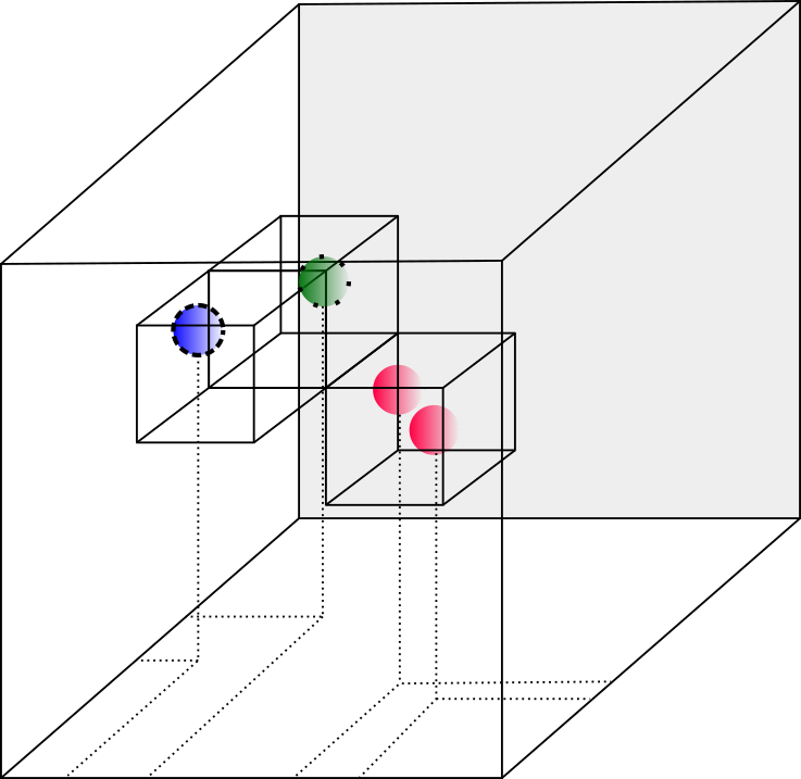
Figure 1: Dynamically discretizing the feasible region (large cube) in $n=3$. We have four search points (the four spheres) each lying in a small cube, or sub-region. Two search points that are close, such as the two red spheres without an outline, can share the same sub-region. While the feasible region can be discretized into more sub-regions, we only have three sub-regions, each containing at least one search point.

To close this section, we need to extend one of the assumptions to the approximate function $\underline{F}_{i}^{k}$ defined in Eq. 8. This will help us later when we want to show for any two points in the same sub-region, their function evaluations cannot differ by too much. The proof is nearly identical to [16, Lemma 2], hence we skip it.

Lemma 2.5.

For $k\geq 1$, there exists $\underline{M}$ s.t. for all $i=1,\ldots,N$,

$$|\underline{F}^{k}_{i}(x)-\underline{F}^{k}_{i}(x^{\prime})|\leq\underline{M}\|x-x^{\prime}\|,\ \forall x,x^{\prime}\in\mathcal{X}_{i}.$$

2.3 Convergence analysis

We will now establish a non-asymptotic convergence guarantee of EDDP (Algorithm 1) for approximately solving the SAA Problem 6. We start by showing $\underline{V}^{k}$ and $\underline{F}^{k}_{i}$ underestimate $V$ and $F_{i}$, respectively, which is similar to [16, Lemma 5]. It will be helpful to recall the definition of cost-to-go function for scenario $i$, $v_{i}$, in Eq. 6, as well as its underestimation $\tilde{v}_{i}^{k}$ defined in Eq. 8.

Lemma 2.6.

For any iteration $k\geq 1$ and scenario $i=0,\ldots,N$,

$$\underline{V}^{k-1}(x)\leq\underline{V}^{k}(x)\leq\frac{1}{N}\sum\limits_{j=1}^{N}\tilde{v}_{j}^{k}(x)\leq V(x) \ \forall x\in\mathcal{X}(\bar{\epsilon})$$ (12)

$$\underline{F}^{k-1}_{i}(x)\leq\underline{F}^{k}_{i}(x)\leq F_{i}(x) \ \forall x\in\mathcal{X}(\bar{\epsilon}).$$ (13)

Proof.

Assuming Eq. 12 holds, then Eq. 13 follows by definition of $F_{i}$ and $\underline{F}^{k}_{i}$ (see Eq. 6 and Eq. 8). The bound $\underline{V}^{k-1}\leq\underline{V}^{k}$ is a direct consequence of the definition of $\underline{V}^{k}$, which recall is

$$\underline{V}^{k}(x)=\max\{\underline{V}^{k-1}(x),\mathrm{cut}^{k}(x)\},$$

where $\mathrm{cut}^{k}(x):=\frac{1}{N}\sum\limits_{i=1}^{N}\tilde{v}_{i}^{k}(x^{k-1})+\langle(\tilde{v}^{k}_{i})^{\prime}(x^{k-1}),x-x^{k-1}\rangle$ is a supporting hyperplane. To show the remaining inequalities, we proceed by induction on the iteration $k$. For the base case $k=1$, we use the fact $\underline{V}^{0}$ lower bounds $V$ over $\mathcal{X}$ (Line 2) to show

$$\frac{1}{N}\sum\limits_{i=1}^{N}\tilde{v}_{i}^{1}(x) =\frac{1}{N}\sum\limits_{i=1}^{N}\min_{x^{\prime}\in X(x,\tilde{\xi}_{i})}\left\{h(x^{\prime},\tilde{c}_{i})+\lambda\underline{V}^{0}(x^{\prime})\right\}$$

$$\leq\frac{1}{N}\sum\limits_{i=1}^{N}\min_{x^{\prime}\in X(x,\tilde{\xi}_{i})}\left\{h(x^{\prime},\tilde{c}_{i})+\lambda V(x^{\prime})\right\}=\frac{1}{N}\sum\limits_{i=1}^{N}v_{i}(x)=V(x).$$ (14)

It remains to show $\underline{V}^{1}(x)\leq\sum\limits_{i=1}^{N}\tilde{v}^{1}_{i}(x)$. Since $\underline{V}^{1}(x)$ is the max of two terms, we consider the two cases where it is set to either one.

Case 1. $\underline{V}^{1}(x)=\underline{V}^{0}(x)$. Then by definition of the lower bound $\underline{V}^{0}$ and the fact $X(x^{0},\tilde{\xi}_{i})\subseteq\mathcal{X}$,

$$\underline{V}^{1}(x) =\frac{1}{N(1-\lambda)}\sum\limits_{i=1}^{N}\min_{x^{\prime}\in\mathcal{X}}h(x^{\prime},\tilde{c}_{i})$$

$$\leq\frac{1}{N}\sum\limits_{i=1}^{N}\min_{x^{\prime}\in X(x,\tilde{\xi}_{i})}\left\{h(x^{\prime},\tilde{c}_{i})+\lambda\underline{V}^{0}(x^{\prime})\right\}=\frac{1}{N}\sum\limits_{i=1}^{N}\tilde{v}^{1}_{i}(x).$$

Case 2. $\underline{V}^{k}(x)=\mathrm{cut}^{1}(x)$. Since $\tilde{v}_{i}^{1}$ is a convex function, then

$$\underline{V}^{1}(x) =\frac{1}{N}\sum\limits_{i=1}^{N}\tilde{v}_{i}^{1}(x^{0})+\langle(\tilde{v}_{i}^{1})^{\prime}(x^{0}),x-x^{0}\rangle\leq\frac{1}{N}\sum\limits_{i=1}^{N}\tilde{v}_{i}^{1}(x).$$

This concludes the base case.

Assume the claim holds for iterations $1,2,\ldots,k-1$, and we prove the $k>1$ case. Let $x^{*}_{i}$ be the optimal feasible solution for the optimization problem defined by $v_{i}(x)$. It follows that

$$\frac{1}{N}\sum\limits_{i=1}^{N}\tilde{v}_{i}^{k}(x) \leq\frac{1}{N}\sum\limits_{i=1}^{N}h(x^{*}_{i},\tilde{c}_{i})+\lambda\underline{V}^{k-1}(x^{*}_{i})\leq\frac{1}{N}\sum\limits_{i=1}^{N}h(x^{*}_{i},\tilde{c}_{i})+\lambda V(x^{*}_{i})=V(x),$$

where the first inequality is by the fact $x^{*}_{i}$ is a feasible solution to the optimization problem defined by $\tilde{v}_{i}^{k}$ and the second is by the inductive hypothesis. For the second inequality in Eq. 12, we again consider two cases.

Case 1. $\underline{V}^{k}(x)=\underline{V}^{k-1}(x)$. Recalling the definition of $\tilde{v}_{i}^{k}$ and using the inductive hypothesis to obtain $\underline{V}^{k-2}\leq\underline{V}^{k-1}$, we get

$$\underline{V}^{k}(x)=\underline{V}^{k-1}(x)\equiv\frac{1}{N}\sum\limits_{i=1}^{N}\tilde{v}^{k-1}_{i}(x)\leq\frac{1}{N}\sum\limits_{i=1}^{N}\tilde{v}^{k}_{i}(x).$$

Case 2. $\underline{V}^{k}(x)=\mathrm{cut}^{k}(x)$. The proof is identical to the base case, hence we skip. ∎

The next result shows a search point becomes saturated (Definition 2.1) when all of its trial points, $x^{k}_{i}$, are saturated. This result is similar to [16, Proposition 4], where we use the data structure $\mathcal{S}$ instead. Since $\mathcal{S}$ changes between iterations, we say $\mathcal{S}^{k}$ is $\mathcal{S}$ at the beginning of iteration $k$ (or end of iteration $k-1$).

Proposition 2.7.

Let $\epsilon_{t}$ follow the recursive definition $\epsilon_{t-1}=(M+\underline{M})\epsilon+\lambda\epsilon_{t}$ and $\epsilon_{T-1}$ be defined so that for any iteration, every point in $\mathcal{X}$ is $\epsilon_{T-1}$-saturated. Let $k\geq 1$.

1. If $\max_{i\in\{0,\ldots,N\}}\mathcal{S}^{k}(x^{k}_{i})\leq t$ for some $t\geq 1$, then for all $i=0,\ldots,N$,

   $$F_{i}(x_{i}^{k})-\underline{F}_{i}^{k}(x_{i}^{k})=\lambda\left[V(x_{i}^{k})-\underline{V}^{k-1}(x_{i}^{k})\right]\leq\epsilon_{t-1}.$$ (15)

   Moreover, $x^{k-1}$ is $\epsilon_{t^{\prime}-1}$-saturated for all $t^{\prime}\geq t$, i.e.,

   $$V(x^{k-1})-\underline{V}^{k}(x^{k-1})\leq\epsilon_{t^{\prime}-1}.$$ (16)

2. If $t=\mathcal{S}^{k}(x)$ for some $x\in\mathcal{X}$, then there exists a solution $x^{\prime}\in\mathcal{X}$ that is $\epsilon_{t^{\prime}}$-saturated for all $t^{\prime}\geq t$ and $\|x-x^{\prime}\|\leq\epsilon$.

Proof.

We prove this using mathematical induction on the iteration index $k$. Starting with the base case of $k=1$, recall that we initialized $\mathcal{S}(x)=T-1$ for all $x\in\mathcal{X}$ in Line 2. By the assumption every point in $\mathcal{X}$ is $\epsilon_{T-1}$-saturated, we have part (b) with $x=x^{\prime}$. Similarly, $\max_{i}\mathcal{S}(x^{k}_{i})=T-1$, and then Eq. 15 is a direct result of the definition of $\epsilon_{T-2}$ and the fact every point in $\mathcal{X}$ is $\epsilon_{T-1}$-saturated. Let $x^{k}_{i}$ be the optimal feasible solution such that $\tilde{v}_{i}^{k}(x^{k-1})=\underline{F}_{i}^{k}(x_{i}^{k})$. Then

$$V(x^{k-1})\equiv\frac{1}{N}\sum\limits_{i=1}^{N}\min_{x\in X(x^{k-1},\tilde{\xi}_{i})}F_{i}(x)\leq\frac{1}{N}\sum\limits_{i=1}^{N}F_{i}(x^{k}_{i}).$$ (17)

We also have by definition of $\underline{V}^{k}$ (Line 12),

$$\underline{V}^{k}(x^{k-1})\geq\frac{1}{N}\sum\limits_{i=1}^{N}\tilde{v}_{i}^{k}(x^{k-1})=\frac{1}{N}\sum\limits_{i=1}^{N}\underline{F}_{i}^{k}(x^{k}_{i}).$$ (18)

Combining the two inequalities above with Eq. 15 yields

$$V(x^{k-1})-\underline{V}^{k}(x^{k-1}) \leq\frac{1}{N}\left(\sum\limits_{i=1}^{N}F_{i}(x_{i}^{k})-\sum\limits_{i=1}^{N}\underline{F}_{i}^{k}(x_{i}^{k})\right)\leq\epsilon_{t-1}.$$

This verifies Eq. 16 and completes the base case of $k=1$.

Now let $k\geq 2$, and suppose the claim holds for all prior iterations. We start by proving part (b). Suppose $t=\mathcal{S}^{k}(x)<T-1$, otherwise if it is equal to $T-1$ we can use the base case argument. Since $\mathcal{S}^{k}(x)=t$ at the beginning of iteration $k$, we must have set $\mathcal{S}(x^{j-1})=t$ in Line 14 during a previous iteration $j<k$ for the first time because this is the only line that updates $\mathcal{S}$, where $x^{j-1}$ and $x$ belong to the same sub-region. Lying in the same sub-region, which is a hypercube with length $\epsilon/\sqrt{n}$, implies $\|x-x^{j-1}\|_{2}\leq\epsilon$. Now, the algorithm sets $\mathcal{S}(x^{j-1})=t$ in Line 14 when $\max_{i=0,\ldots,N}\mathcal{S}^{j}(x^{j}_{i})\equiv t^{*}=t+1$. Using the inductive hypothesis of part (a), then $x^{\prime}=x^{j-1}$ is $\epsilon_{t^{\prime}}$-saturated for all $t^{\prime}\geq t$ and its (Euclidean) distance to $x$ is at most $\epsilon$.

Next, we prove part (a) for iteration $k\geq 2$. The assumption $\max_{i}\mathcal{S}^{k}(x^{k}_{i})\leq t$ implies that for each scenario $i$ there is a saturation level $t_{i}$ such that $\mathcal{S}(x^{k}_{i})=t_{i}\leq t$. Applying part (b) to each $x^{k}_{i}$, then there exists a previous search point $x^{j_{i}-1}$ that is $\epsilon_{t^{\prime}}$-saturated for all $t^{\prime}\geq t_{i}$ and $\|x^{k}_{i}-x^{j_{i}-1}\|\leq\epsilon$. As a result,

$$\begin{split}&F_{i}(x_{i}^{k})-\underline{F}_{i}^{k}(x_{i}^{k})\\ &\leq F_{i}(x_{i}^{k})-\underline{F}^{j_{i}+1}(x_{i}^{k})\\ &=\left[F_{i}(x_{i}^{k})-F_{i}(x^{j_{i}-1})\right]+\left[F_{i}(x^{j_{i}-1})-\underline{F}_{i}^{j_{i}+1}(x^{j_{i}-1})\right]+\left[\underline{F}_{i}^{j_{i}+1}(x^{j_{i}-1})-F^{j_{i}+1}(x_{i}^{k})\right]\\ &\leq(M+\underline{M})\|x_{i}^{k}-x^{j_{i}-1}\|+\lambda\left[V(x^{j_{i}-1})-\underline{V}^{j_{i}}(x^{j_{i}-1})\right]\\ &\leq(M+\underline{M})\epsilon+\lambda\epsilon_{t^{\prime}}=\epsilon_{t^{\prime}-1},\end{split}$$ (19)

where the first inequality is by Lemma 2.6, the second is by continuity of $F_{i}$ and $\underline{F}_{i}$, and the last is by $x^{j_{i}-1}$ being $\epsilon_{t^{\prime}}$-saturated for all $t^{\prime}\geq t$. Since $t_{i}\leq t$, this proves Eq. 15. We can prove Eq. 16 in a similar fashion to the base case, so we omit this step. This completes the inductive step, and so the result holds for all $k\geq 1$. ∎

In the previous proposition, we assumed every search point is $\epsilon_{T-1}$-saturated. The following lemma provides a value to $\epsilon_{T-1}$. Recall $\lambda\in(0,1)$ is the discount factor, $D$ is the length of the feasible region (Assumption 2.1) and $M_{h}$ is the Lipschitz constant of the cost function $h$ (Assumption 2.3).

Lemma 2.8.

For any $k\geq 0$ and $x\in\mathcal{X}$,

$$V(x)-\underline{V}^{k}(x)\leq\frac{M_{h}D}{1-\lambda}.$$

Proof.

Observe the cost-to-go function from Problem 6 can be rewritten as

$$V(x)=\frac{1}{N}\sum\limits_{i=1}^{N}\min_{x_{i}\in X(x,\tilde{\xi}_{i})}\{h(x_{i},\tilde{c}_{i})+\lambda V(x_{i})\}.$$

By definition of $\underline{V}^{0}$ in Line 2, we similarly have

$$\underline{V}^{0}(x) =\frac{1}{N}\sum\limits_{i=1}^{N}\sum\limits_{t=0}^{\infty}\lambda^{t}\cdot\min_{x_{i}\in\mathcal{X}_{i}}\left\{h(x_{i},\tilde{c}_{i})\right\}=\frac{1}{N}\sum\limits_{i=1}^{N}\min_{x_{i}\in\mathcal{X}_{i}}\big{\{}h(x_{i},\tilde{c}_{i})+\lambda\underbrace{\sum\limits_{t=0}^{\infty}\lambda^{t}\cdot h(x_{i},\tilde{c}_{i})}_{\underline{V}^{0}(x_{i})}\big{\}}.$$

Let $\bar{x}_{i}$ and $\hat{x}_{i}$ be the optimal solution to scenario $i$ in $V(x)$ and $\underline{V}^{0}(x)$ as defined above, respectively. Then

$$V(x)-\underline{V}^{k}(x) \leq V(x)-\underline{V}^{0}(x)$$

$$=\frac{1}{N}\sum\limits_{i=1}^{N}[h(\bar{x}_{i},\tilde{c}_{i})-h(\hat{x}_{i},\tilde{c}_{i})]+\lambda[V(\bar{x}_{i})-\underline{V}^{0}(\hat{x}_{i})]$$

$$\leq\frac{1}{N}\sum\limits_{i=1}^{N}M_{h}\|\bar{x}_{i}-\hat{x}_{i}\|+\lambda[V(\bar{x}_{i})-\underline{V}^{0}(\hat{x}_{i})]$$

$$\leq M_{h}D+\frac{\lambda}{N}\sum\limits_{i=1}^{N}[V(\bar{x}_{i})-\underline{V}^{0}(\hat{x}_{i})],$$

where the first inequality is by Lemma 2.6, the second inequality is by definition of $\underline{V}^{0}$, the third inequality is by $h$ being $M_{h}$-Lipschitz and domain length being bounded by $D$. Repeating this argument and using boundedness of $V(x)$ and $\underline{V}^{0}(x^{\prime})$ for all $x,x^{\prime}\in\mathcal{X}$, we obtain the desired inequality. ∎

We now bound the number of EDDP iterations. Recall $\mathcal{S}$ consists of $\left(D\sqrt{n}/\epsilon+1\right)^{n}$ sub-regions, or hypercubes, with side length $\epsilon/\sqrt{n}$, and each is assigned a value between $0$ and $T-1$ (inclusively). Let us define $|\mathcal{S}|$ as the sum of the values from every sub-region, which only decreases during Algorithm 1. If the algorithm has not terminated, there exists a point $x\in\mathcal{X}$ where $\mathcal{S}(x)\geq 1$, or equivalently, $1\leq|\mathcal{S}|\leq(T-1)(D\sqrt{n}/\epsilon+1)^{n}$. We will show $|\mathcal{S}|$ decreases by at least one during iterations $\{\ell T+1,\ldots,(\ell+1)T\}$ for any integer $\ell\geq 0$ in the following lemma, which is similar to [16, Proposition 5]. Recall $\mathcal{S}^{k}$ is $\mathcal{S}$ at the beginning of iteration $k$.

Lemma 2.9.

Let $k=\ell T+1$ for some nonnegative integer $\ell$. EDDP either terminates during iteration $k$ or generates a search point $x^{k+t-2}$ at iteration $k+t-2$ satisfying $\mathcal{S}^{k+t-2}(x^{k+t-2})\geq t$ and $\mathcal{S}^{k+t}(x^{k+t-2})\leq t-1$ for some $t$ where $2\leq t\leq T-1$.

Proof.

First, recall every search point $x\in\mathcal{X}$ has its saturation level set to $T-1$, i.e. $\mathcal{S}^{1}(x)=T-1$. Noting that we only decrease $\mathcal{S}(x)$, then $\mathcal{S}^{j}(x)\leq T-1$ for every iteration $j$ and search point $x\in\mathcal{X}$. Then similar to [16, Proposition 5], we consider the following $T-1$ cases, one of which must occur at the $k$-th iteration of EDDP:

1. Case 1: $\mathcal{S}^{k}(x^{k})\leq 1$

2. Case $t$, $t=2,\ldots,T-1$: $\mathcal{S}^{k+t-2}(x^{k+t-2})\geq t$ and $\mathcal{S}^{k+t-1}(x^{k+t-1})\leq i,\ \forall t\leq i\leq T-1$

We start with the first case. Observe our choice of $k$ implies $(k+1)\text{ mod }T\not\equiv 1$. Then Line 13 sets

$$x^{k}=\mathrm{argmax}_{\{x_{i}^{k}\}_{i\geq 0}}\mathcal{S}^{k}(x^{k}_{i}).$$

Therefore, by definition of $t^{*}=\max_{i\geq 0}\mathcal{S}^{k}(x_{i}^{k})$ in Line 8 and the assumption $\mathcal{S}^{k}(x^{k})\leq 1$, we have $t^{*}\leq 1$, which implies we terminate in Line 9 during iteration $k$.

We now consider the $t$-th case where $2\leq t\leq T-1$. For notational convenience, define $k^{\prime}=k+t-1$. For reasons similar to the first case, we get $t^{*}=\max_{i\geq 0}\mathcal{S}^{k^{\prime}}(x^{k^{\prime}}_{i})\leq t$ during iteration $k^{\prime}$. Combining with the fact Line 14 updates

$$\mathcal{S}(x^{k^{\prime}-1})=\min(\mathcal{S}(x^{k^{\prime}-1}),\max(0,t^{*}-1))$$

during iteration $k^{\prime}$, we can conclude $\mathcal{S}(x^{k^{\prime}-1})\leq t-1$ during iteration $k^{\prime}$, which implies $\mathcal{S}^{k^{\prime}+1}(x^{k^{\prime}-1})\leq t-1$. Recalling the assumption $\mathcal{S}^{k+t-2}(x^{k+t-2})\geq t$ completes the proof for case $t$. ∎

We are now ready to establish the number of iterations of EDDP (Algorithm 1) to obtain a feasible solution $x^{k}_{0}\in X(x^{0},\xi_{1})$ to the SAA problem (Problem 6) satisfying

$$F(x^{k}_{0})-F^{*}\leq\epsilon_{0},$$

where $F^{*}\equiv F(x^{*})=\min_{x\in X(x_{0},\xi_{0})}F(x)$ is the optimal value and $\epsilon_{t}$ is defined recursively from Proposition 2.7.

Theorem 2.10.

Fix an effective planning horizon $T\geq 2$ and parameter $\epsilon\in(0,D)$ so that the length of each sub-region is $\epsilon/\sqrt{n}$, where $n$ is the size of the decision vector and $D$ is the length of the domain. Let $\epsilon_{t}$ be defined by

$$\epsilon_{t}=\begin{cases}\displaystyle(1-\lambda)^{-1}M_{h}D&t=T-1\\ \sum_{\tau=t}^{T-2}\left[\left(M+\underline{M}\right)\epsilon\right]\lambda^{\tau-t}+\lambda^{T-t-1}\epsilon_{T-1},&0\leq t\leq T-2\end{cases},$$ (20)

where $M$, $M_{h}$, and $\underline{M}$ are, respectively, the Lipschitz constants for $F_{i}$, $h(\cdot,\tilde{c}_{i})$, and $\underline{F}_{i}$ over scenarios $i=0,\ldots,N$. Then EDDP returns a feasible solution $x^{k}_{0}$ such that

$$F(x^{k}_{0})-F^{*}\leq\epsilon_{0}\leq\frac{(M+\underline{M})(1-\lambda^{T-1})}{1-\lambda}\epsilon+\frac{\lambda^{T-1}}{1-\lambda}M_{h}D$$ (21)

in at most $K$ iterations, where

$$K:=T(T-1)\left(D\sqrt{n}/\epsilon+1\right)^{n}.$$

Proof.

The number of iterations follows from the discussion made before Lemma 2.9 and the fact every $T$ iterations $|\mathcal{S}|$ decreases by one thanks to Lemma 2.9.

Now we show the algorithm returns a feasible solution $x^{k}_{0}$ that has a function gap at most $\epsilon_{0}$. First, we check feasibility. Recall that $x^{k}_{0}\in X(x_{0},\tilde{\xi}_{0})$. Since we defined $\tilde{\xi}_{0}=\xi_{1}$, then we have that $x_{0}^{k}$ is a feasible solution. For optimality of $x^{k}_{0}$, we have by the termination criterion that $t^{*}=1$ (Line 9). In other words, $\max_{0\leq i\leq N}\mathcal{S}(x^{k}_{i})=1$, which in view of Proposition 2.7 and definition of $\epsilon_{t}$ implies

$$F_{0}(x^{k}_{i})-\underline{F}_{0}^{k}(x^{k}_{i})\leq\epsilon_{0} =\sum_{\tau=0}^{T-2}\left[\left(M+\underline{M}\right)\epsilon\right]\lambda^{\tau}+\frac{\lambda^{T-1}}{1-\lambda}M_{h}D$$

$$=\frac{(M+\underline{M})(1-\lambda^{T-1})}{1-\lambda}\epsilon+\frac{\lambda^{T-1}}{1-\lambda}M_{h}D.$$

Since $F_{0}=F$ by definition of scenario $\tilde{\xi}_{0}$, we conclude

$$F(x^{k}_{0})-\underline{F}_{0}^{k}(x^{k}_{0})\geq F(x^{k}_{0})-\underline{F}_{0}^{k}(x^{*})\geq F(x^{k}_{0})-F(x^{*}),$$

where the first inequality is by optimality of $x^{k}_{0}$ and the second is by $\underline{F}_{0}^{k}\leq F$ thanks to Lemma 2.6. ∎

Setting $\epsilon=\frac{\varepsilon(1-\lambda)}{2(M+\underline{M})}$ and $T=\ln(\frac{M_{h}D}{\varepsilon(1-\lambda)})/(1-\lambda)$, then $F(x^{k}_{0})-F^{*}\leq\varepsilon$ for any $\varepsilon>0$. Thus, the effective planning horizon $T$ has a logarithmic dependence on the final accuracy $\varepsilon$ while it has a nearly linear dependence on the inverse of $1-\lambda$. While previous works show their algorithm has a linear dependence on $T$, c.f. [16, Theorem 2], these works define one iteration as a forward phase plus a backward phase. Every forward (resp. backward) phase consists of $T$ forward (resp. backward) steps, and each step involves solving $N$ subproblems of the form Eq. 8. Therefore, a better measure of complexity is the number of steps from a forward or a backward phase. In this case, the number of iterations is proportional to $2T^{2}$, which matches our complexity result up to a constant. Indeed, we can save the factor of two since we seem to merge the forward and backward phases into one iteration. In the next section, we show by changing just three lines in EDDP, we can improve the dependence of the effective planning horizon.

2.4 Reducing dependence on the effective planning horizon

To reduce the dependence of $T$ from quadratic to linear, we do not explicitly reset the search point, i.e., set $x^{k}=x^{0}$ every $T$ iterations in Line 13. Rather, we implicitly reset every iteration. We modify subproblem $i=0$ so that the previous search point is always $x^{0}$ while the remaining $N$ subproblems use the last iteration’s most distinguishable search point, $x^{k-1}$. Implementing this idea requires modification of three lines, as shown by Algorithm 2. The first change of Line 6 only modifies the feasible region of subproblem $i=0$ to use $x^{0}$ instead of $x^{k-1}$ as the previous search point. The motivation for this change is to approximately solve the original problem, Problem 6, which is

$$\min_{x\in X(x^{0},\xi_{1})}F(x),$$

every iteration. Compare this with the previous EDDP, where we solve the above problem every $T$ iterations by choosing the next search point to $x^{k}=x^{0}$. Consequently, we can check whether we have an approximately optimal solution every iteration instead of waiting for $T$ iterations. The second modification in Line 9, which removes the conditional of $k~{}\mathrm{mod}~{}T\equiv 1$ in order to terminate, reflects the fact we solve the original problem every iteration. Finally, since we do not explicitly reset every $T$ iterations, we can simplify Line 13 to not set $x^{k}=x^{0}$.

Algorithm 2

1:procedure Faster Infinite-Horizon EDDP

2:     Run EDDP (Algorithm 1) but modify Eq. 8 (in Line 6) into

$$\tilde{v}^{k}_{i}(x^{k-1})=\min_{x\in\scriptsize\begin{cases}X(x^{0},\tilde{\xi}_{0}):i=0\\ X(x^{k-1},\tilde{\xi}_{i}):i\geq 1\end{cases}}\left\{\underline{F}^{k}_{i}(x):=h(x,\tilde{c}_{i})+\lambda\underline{V}^{k-1}(x)\right\}.$$ (22)

3:     Modify Line 9 into

if $$t^{*}=1$$ then

4:     Modify Line 13 to

$$x^{k}=\mathrm{argmax}_{\{x_{i}^{k}\}_{i=0}^{N}}\ \mathcal{S}(x^{k}_{i})$$ (23)

5:end procedure

We now analyze the convergence of the modified EDDP algorithm. It can be checked that the only two results for proving the convergence of Algorithm 1 affected by this modification are Lemma 2.9 and Theorem 2.10. For comparison, Lemma 2.9 can only be applied to every $T$ iterations. Below, we develop a similar lemma that can be applied to every iteration. We skip the proof since it is nearly identical to the proof of Lemma 2.9.

Lemma 2.11.

For any $k\geq 1$, the modified EDDP (Algorithm 2) either terminates during iteration $k$ or generates a search point $x^{k+t-2}$ at iteration $k+t-2$ satisfying $\mathcal{S}^{k+t-2}(x^{k+t-2})\geq t$ and $\mathcal{S}^{k+t}(x^{k+t-2})\leq t-1$ for some $t$ where $2\leq t\leq T-1$, assuming we have not terminated by the beginning of iteration $k+T$.

The additional assumption of not terminating by the beginning of iteration $k+T-1$ is to ensure the algorithm can still decrease $\mathcal{S}$ during iteration $k+T-1$. The above lemma can be used as follows. For each iteration $1,2,\ldots k_{0}$, we invoke the lemma to, ideally, decrease $|\mathcal{S}|$ by $k_{0}$, where $k_{0}\geq 1$ is some iteration index. Compare this with our discussion prior to Lemma 2.9, where we can only decrease $|\mathcal{S}|$ by $\lfloor k_{0}/T\rfloor$. We formalize this below, where the proof only looks at odd or even indices to avoid double counting. For a visual companion to the proof, see Figure 2.

Lemma 2.12.

Fix a $k_{0}\geq 1$. Assuming the modified EDDP has not terminated by the beginning of iteration $k_{0}+T$, then from iteration $1$ to $k_{0}+T-2$, $|\mathcal{S}|$ decreases by at least $\lceil k_{0}/2\rceil$.

Proof.

For $k=1,\ldots,k_{0}$, we say the iteration $k+t-2$ satisfying the properties of Lemma 2.11 is the target iteration of $k$. The list of all target iterations can be split into even or odd indices. Let $I$ be the subset of target iterations where at least half of the iterations $k$ from $1\leq k\leq k_{0}$ have their target iteration in $I$.

For each target iteration $i\in I$, there exists a set of $L$ iterations $\{k_{j}\}_{j=1}^{L}$ (without loss of generality, a strictly increasing sequence) that have the same target iteration, $i=k_{j}+t_{j}-2$, where $L$ is some positive integer where $1\leq L\leq T-1$ and $\{t_{j}\}_{j=1}^{L}\subseteq\{2,\ldots,T-1\}$ is a set of integers that ensure $k_{j}+t_{j}-2=i$. One can also check $\{t_{j}\}$ is decreasing, and so $t_{1}$ and $t_{L}$ are the largest and smallest values from the set, respectively. By invoking Lemma 2.11 to iterations $k_{1}$ and $k_{L}$, we find $\mathcal{S}^{i}(x^{i})\geq t_{1}$ and $\mathcal{S}^{i+2}(x^{i})\leq t_{L}-1$. In other words, $\mathcal{S}(x^{i})$ decreased by at least $t_{1}-t_{L}+1$ during iterations $i$ and $i+1$. Since $L\leq t_{1}-t_{L}+1$ because $\{t_{j}\}_{j=1}^{L}$ are strictly decreasing integers, we can conclude $\mathcal{S}(x^{i})$ decreased by at least $L$ during those two iterations.

We repeat this argument for all target iterations $i\in I$. Therefore, $|\mathcal{S}|$ must have decreased by the number of iterations that have their target iteration in $I$, which is at least half of $k_{0}$. ∎

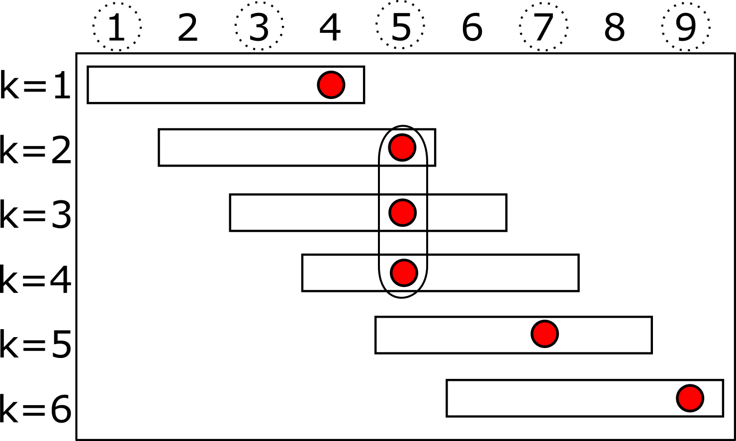
Figure 2: For each iteration $k=1,\ldots,6$ (rows) where $T=5$, there is a rectangle and solid-lined red circle. The solid circle is the target iteration $k+t-2$ (columns) from Lemma 2.11 while the rectangle is the set of possible target iterations. Notice iterations 2, 3, and 4 share the same target iteration 5, highlighted by the oval. Thus, for target iteration $i=5$, there exists $L=3$ iterations $\{2,3,4\}$ that have the same target iteration. Also observe that the odd set of target iterations, $I=\{1,3,5,7,9\}$, contains 5 out of 6 target iterations. So we choose this $I$ in Lemma 2.12, indicated by the dotted circles.

The above lemma asserts we can on average decrease $|\mathcal{S}|$ by at least one every two iterations rather than once every $T$ iterations. This more frequent decreasing of $\mathcal{S}$ leads to the improved iteration complexity in the next theorem.

Theorem 2.13.

Let everything be defined as in Theorem 2.10. Running the modified EDDP we get a feasible solution $x^{k}_{0}$ such that

$$F(x^{k}_{0})-F^{*}\leq\epsilon_{0}\leq\frac{(M+\underline{M})(1-\lambda^{T-1})}{1-\lambda}\epsilon+\frac{\lambda^{T-1}}{1-\lambda}M_{h}D,$$

but now the number of iterations is at most

$$K:=2(T-1)(D\sqrt{n}/\epsilon+1)^{n}+(T+1).$$

Proof.

The proof is largely the same as Theorem 2.10. The main difference is that we can reduce the number of iterations by about a factor of $T/2$ thanks to Lemma 2.12, where the additional $T+1$ iterations come from the fact the algorithm may not terminate until the iteration $k_{0}+T$ in Lemma 2.12 for some $k_{0}$. ∎

Compared to Theorem 2.10, the number of iterations is reduced by about $T/2$ without significantly modifying the structure of EDDP for solving the infinite-horizon problem. It is also possible to provide an improvement to EDDP for solving the finite-horizon problem from [16], but it requires a different set of modifications. The main idea is to skip a step of the backward phase after a step of the forward phase if the next search point $x^{k}$ is $\epsilon_{t}$-saturated for some $t$. This modification is proposed by the nonconsecutive dual dynamic programming method developed in [37] for solving finite-horizon problems. However, this modification alters the structure of EDDP. For example, an iteration involves an additional “if else” statement and may skip the backward phase. On the other hand, our modifications to EDDP preserve the algorithmic structure. It seems our modifications exploit the fact the infinite-horizon problem is stationary.

3 Hierarchical dual dynamic programming

In this section, we consider solving a so-called hierarchical stationary stochastic program. The problem is defined as the stochastic program over an infinite horizon from Problem 1, where the cost function is now a stochastic two-stage program,

$$h(x,c):=\min_{z_{1}\in Z_{1}(x,c^{1})}f^{1}(z^{1},\ell^{1})+\mathbb{E}\big{[}\min_{z^{2}\in Z^{2}(z^{1},c^{2})}f^{2}(z^{2},\ell^{2})\big{]},$$ (24)

with the parametric feasibility sets

$$Z^{k}(u,c^{k}) :=\{z\in\bar{Z}^{k}\subseteq\mathbb{R}^{n_{k}},:A^{k}z-B^{k}u-b^{k}\in\mathcal{K}^{k}\},\ ~{}k\in\{1,2\},$$ (25)

where $\bar{Z}^{k}$ is a closed convex set and $\mathcal{K}^{k}$ is a regular cone for $k\in\{1,2\}$. The vectors are defined as $c^{k}=\{A^{k},B^{k},b^{k},\ell^{k}\}$ for $k\in\{1,2\}$ with linear mappings $A^{k}:\mathbb{R}^{n_{k}}\to\mathbb{R}^{m_{k}}$ for $k\in\{1,2\}$, $B^{1}:\mathbb{R}^{n}\to\mathbb{R}^{m_{1}}$, and $B^{2}:\mathbb{R}^{n_{1}}\to\mathbb{R}^{m_{2}}$. Recall that $n$ is the dimension of the variable in the infinite-horizon problem. The expectation is taken w.r.t. the random variable $c^{2}$. The functions $f^{k}(\cdot,\ell^{k}):\mathbb{R}^{n^{k}}\to\mathbb{R}$ are relatively simple, closed, and convex and parameterized by the vector $\ell^{k}$ for $k\in\{1,2\}$. When conditioning on the (possibly random) vector $c$, we assume $c^{1}$ is fixed while $c^{2}$ is random and possibly dependent on $c^{1}$. From this definition, $h(\cdot,c)$ is a closed convex function for any fixed vector $c$ as long as Problem 24 is feasible, which we assume throughout this section.

We refer to the infinite-horizon problem (Problem 1) and stochastic two-stage problem (Problem 24) as the top-level and lower-level problem, respectively. Note that the dimension of the top-level problem need not be the same as the lower-level problem, and in many cases, can be much smaller. That is, $n\ll\min\{n_{1},n_{2}\}$.

This class of hierarchical stationary stochastic programs captures planning problems with a hierarchy of decision-making. The decision variable $x^{t}$ from the top-level problem can be viewed as high-level decisions, e.g., long-term, big-picture planning. At each time $t$, the variables $z_{1}$ and $z_{2}$, determined by the decision maker in the lower-level problem, can be viewed as low-level decisions, e.g., operational decisions. The main difficulty in solving the above stochastic two-stage program is we cannot solve it exactly in general. We consider solving its SAA problem instead. To solve the SAA problem, one can use an LP solver if the cost functions and constraints are linear. However, if the number of samples or decision variable sizes $n_{1}$ or $n_{2}$ are large, this problem can be prohibitively large. Alternatively, one can solve the above problem using first-order methods, such as the recently developed dynamic stochastic approximation method [19]. In the next subsection, we propose a similar first-order method.

3.1 Solving the subproblem via inexact primal-dual stochastic approximation

We propose a primal-dual algorithm to approximately solve the subproblems in a hierarchical stationary stochastic program. We solve each subproblem by replacing the expectation in the lower-level problem with an empirical average using $N_{2}$ samples. In contrast, we reserve $N_{1}\equiv N$ to be the number of samples for the top-level problem. First, we need to make some assumptions regarding the top-level problem. We assume that the set $X(x^{k-1},\tilde{\xi}_{i})$, as defined in Eq. 2, is easy to project onto for any $x^{k-1}\in\mathcal{X}$ and sample $\tilde{\xi}_{i}$. In addition, we assume for simplicity there are no functional constraints, i.e, the functional $\Phi(x,r)$ is empty in Eq. 2. Also suppose that in addition to the regularity conditions of the top-level problem (Assumption 2.2), the strong Lagrange duality holds for the lower-level problem. Then subproblem $i$ of EDDP at iteration $k$ can be approximated by the saddle point problem,

$$\begin{split}\min_{\begin{subarray}{c}x\in X(x^{k-1},\tilde{\xi}_{i})\\ z^{1}\in\bar{Z}_{1}\end{subarray}}\ \max_{\begin{subarray}{c}\alpha\in\mathcal{K}_{*}\\ \beta\in\mathcal{K}^{1}_{*}\end{subarray}}\ &f_{1}(z^{1},\ell_{1})+\langle\alpha,\tilde{A}_{i}x-\tilde{B}_{i}x^{k-1}-\tilde{b}_{i}\rangle+\langle\beta,\tilde{A}^{1}_{i}z^{1}-\tilde{B}^{1}_{i}x-\tilde{b}^{1}_{i}\rangle\\ &\hskip 5.0pt+\frac{1}{N_{2}}\sum\limits_{j=1}^{N_{2}}v_{2,j}(x,z^{1}),\end{split}$$ (26)

where for $j=1,\ldots,N_{2}$,

$$v_{2,j}(x,z^{1}):=\lambda\underline{V}^{k}(x)+\min_{z^{2}_{j}\in Z_{2}(z^{1},c_{j}^{2})}\{f_{2}(z^{2}_{j},\ell^{2}_{j})\}.$$

Here, $\underline{V}^{k}$ is the cutting-plane model defined according to Eq. 9, which is a piecewise linear function. Similar to how the $i$-th sample from the top-level problem is $\tilde{\xi}_{i}=\{\tilde{A}_{i},\tilde{B}_{i},\tilde{Q}_{i},\tilde{b}_{i},\tilde{c}_{i},\tilde{r}_{i}\}$ (see Eq. 5), we denote the corresponding $i$-th sample vector $c^{1}$ from Eq. 25 as $c^{1}\equiv\tilde{c}^{1}_{i}=\{\tilde{A}^{1}_{i},\tilde{B}^{1}_{i},\tilde{b}^{1}_{i},\tilde{\ell}^{1}_{i}\}$ since we assumed $c^{1}$ to be fixed when conditioned on the random vector $c$. Similarly, the samples for approximating the expectation in the lower-level problem are $\tilde{c}^{2}_{j}=\{\tilde{A}^{2}_{j},\tilde{B}^{2}_{j},\tilde{b}^{1}_{j},\tilde{\ell}^{1}_{j}\}$. Recall the scalar $\lambda\in(0,1)$ is the discount factor. We place $\underline{V}^{k}(x)$ inside $v_{2,j}$ rather than write it directly in the saddle point problem since it is relatively easy to take the subgradient of $\underline{V}^{k}$, whereas optimizing $\underline{V}^{k}$ with a prox-mapping is more challenging.

Remark.

While it may seem redundant to project onto $X(x^{k-1},\tilde{\xi})$ and include the dual multiplier $\alpha\in\mathcal{K}_{*}$ for the constraint $Ax-Bx^{k-1}-b\in\mathcal{K}$ in Problem 26, this is done to obtain both a feasible solution $x\in X(x^{k-1},\tilde{\xi})$ and subgradient w.r.t. the previous point $x^{k-1}$ via the dual multiplier. If $X(x^{k-1},\tilde{\xi})$ is not easy to project onto, one can replace the constraint of $x\in X(x^{k-1},\tilde{\xi})$ in Problem 26 with $x\in\bar{X}$ (defined in Eq. 2). But, one must possibly adjust the constants in the assumptions to hold for the larger feasible set $\bar{X}$ rather than the original feasible set $\mathcal{X}$, e.g., Assumption 2.1.

Problem 26 can be expressed as the generic saddle point problem,

$$v(u,\xi=[W,U,q,\ell]):=\min_{y\in K_{*}}\max_{x\in X}\langle y,q+Uu-Wx\rangle+f(x,\ell)+\mathbb{E}_{\omega}[\tilde{v}(x,\omega)],$$ (27)

where $\xi$ is a fixed set of matrices and vectors, while $K_{*}$ and $X$ are a dual cone and closed convex set, respectively, for some cone $K$. Later, we will set $u=x^{k-1}$, the previous search point from EDDP. The input vector $\ell$ and random vector $\omega$ parameterize the closed convex functions $f(\cdot,\ell)$ and $H(\cdot,\omega)$, respectively. The expectation is taken over the random variable $\omega$, which is an i.i.d. uniform random variable that samples from the set $\{1,\ldots,N_{2}\}$ and $\tilde{v}(\cdot,i)\equiv v_{2,i}(\cdot)$.

Before solving the generic saddle point problem, we need to introduce some notation. For a closed convex set $X$, a function $\omega_{X}:X\to R$ is called a distance generating function with parameter $\alpha_{X}$, if $\omega_{X}$ is continuously differentiable and strongly convex with parameter $\alpha_{X}$ w.r.t. an arbitrary norm $\|\cdot\|$. Therefore, we have

$$\left\langle y-x,\nabla\omega_{X}(y)-\nabla\omega_{X}(x)\right\rangle\geq\alpha_{X}\|y-x\|^{2},\forall x,y\in X.$$

The Bregman divergence associated with $\omega_{X}$ is defined as

$$V_{X}(x,y)=\omega_{X}(y)-\omega_{X}(x)-\left\langle\nabla\omega_{X}(x),y-x\right\rangle,\forall x,y\in X.$$

It can be easily seen that $V_{X}(x,y)\geq\frac{\alpha_{X}}{2}\|y-x\|^{2},\forall x,y\in X$. Assuming $X$ is bounded, we define the diameter of the set $X$ as

$$D_{X}^{2}=\max_{x,y\in X}V_{X}(x,y).$$ (28)

For a closed convex cone $K_{*}$, let the distance generating function be $\omega_{K_{*}}(y)=\|y\|^{2}/2$.

To solve the generic saddle point problem, we use Algorithm 3, which is called the (inexact) primal-dual stochastic approximation method, or PDSA. In each iteration, we sample an i.i.d. uniform random variable $i_{k}$ in Line 3 to select a scenario for the lower-level’s second-stage problem, $\tilde{v}(\cdot,i_{k})$. When the number of samples $N_{2}$ is large, sampling can save computational effort. This approach is similar to sampling a subgradient in a randomized primal-dual gradient method from [18]. However, unlike [18], we do not require a bounded dual feasible region in our convergence analysis. Also, we can reuse samples when re-estimating a subgradient of $\mathbb{E}[\tilde{v}(\cdot,\omega)]$. In contrast, the stochastic approximation method in [19] samples a new random variable directly w.r.t. the expectation. Thus, there is no reuse. Reusing samples is useful since we will repeatedly estimate a subgradient of $\mathbb{E}[\tilde{v}(\cdot,\omega)]$. After sampling $i_{k}$, we compute an $\bar{\epsilon}$-subgradient (i.e., inexact if $\bar{\epsilon}>0$ and exact if $\bar{\epsilon}=0$) in Line 4, denoted by $\partial_{\bar{\epsilon}}\tilde{v}(\cdot,i_{k})$. We provide a formal definition in Definition 3.1. If, for example, $\tilde{v}(\cdot,i_{k})$ is defined by another optimization problem, we can compute its subgradient via a black-box solver or a nested call to PDSA. By making nested calls, one derives a so-called dynamic stochastic approximation algorithm [19]. After obtaining the subgradient, the algorithm performs a primal and dual update step. The final output is taken as a convex combination of all previous primal-dual iterates.

1:procedure (Inexact) primal-dual stochastic approximation

2:     for $k=1,\ldots,N$ do

3:         Sample an i.i.d. uniform random variable $i_{k}\sim\{1,\ldots,N_{2}\}$

4:         Let $G_{k-1}$ be an $\bar{\epsilon}$-subgradient of $\tilde{v}(\cdot,i_{k})$, i.e.,

$$G_{k-1}\in\partial_{\bar{\epsilon}}\tilde{v}(x_{k-1},i_{k}).$$

5:         $\tilde{d}=\theta_{k}(y_{k-1}-y_{k-2})+y_{k-1}$

6:         $x_{k}=\underset{x\in X}{\operatorname{argmin}}\langle q+Uu-Wx,\tilde{d}\rangle+f(x,\ell)+\left\langle G_{k-1},x\right\rangle+\tau_{k}V_{X}(x_{k-1},x)$

7:         $y_{k}=\underset{y\in\mathcal{K}_{*}}{\operatorname{argmin}}\left\langle-q-Uu+Wx_{k},y\right\rangle+\frac{\eta_{k}}{2}\|y-y_{k-1}\|^{2}$

8:     end for

9:     $(\bar{x},\bar{y})=(\sum\limits_{k=1}^{N}w_{k})^{-1}\sum\limits_{k=1}^{N}w_{k}\cdot(x_{k},y_{k})$

10:end procedure

Algorithm 3

We will now discuss the convergence of the PDSA method. In [19], convergence results are shown only in expectation. Thus, their results cannot be directly applied to EDDP, since EDDP is a deterministic algorithm. To deal with the randomness, another approach is to show the generated supporting hyperplanes are accurate with high probability. To do so without significantly deteriorating the iteration complexity, we impose a slightly restrictive assumption on the distribution of stochastic gradients, $G_{k-1}\equiv G(x_{k-1},i_{k})$. Specifically, we assume the following “light-tail” assumption, where there is some $\sigma>0$ such that

$$\mathbb{E}\big{[}\mathrm{exp}\{\|G(x,i_{k})-g(x)\|_{*}^{2}/\sigma^{2}\}\big{]}\leq\mathrm{exp}\{1\},~{}\ \forall x\in X,$$ (29)

where $g(x)=\mathbb{E}[G(x,i_{k})]$. This can be satisfied if $\|G(x,i_{k})-g(x)\|_{*}\leq\sigma$ for all $(x,i_{k})\in X\times\Xi$, where $X$ is the domain of the decision variable and $\Xi$ is the support of the random variable. In the case where the expectation is approximated by a finite sum, this assumption is satisfied by $\sigma=2\bar{G}$, where $\bar{G}\geq 0$ is a constant such that

$$\|s_{i}\|\leq\bar{G},~{}\forall s_{i}\in\partial_{\bar{\epsilon}}\tilde{v}(x,i),~{}\forall i\in[N],~{}\forall x\in X.$$ (30)

We will now define a function to measure the accuracy of the primal and dual solution $\bar{z}\equiv(\bar{x},\bar{y})\in Z:=X\times Y$. Suppose a vector $u\in\mathbb{R}^{n}$ is given to us. In this section only, define $\tilde{v}(x)=\mathbb{E}_{\omega}[\tilde{v}(x,\omega)]$ as the expected function appearing in the general saddle-point problem from Eq. 27, which is for notational convenience. We define the following Q-gap function,

$$Q(\bar{z};x,y)=\langle y,q+Uu-W\bar{x}\rangle+h(\bar{x},c)+\tilde{v}(\bar{x})-[\langle\bar{y},q+Uu-Wx\rangle+h(x,c)+\tilde{v}(x)].$$

We can then define the following two gap functions

$$\mathrm{gap}_{*}(\bar{z}) =\max\{Q(\bar{z};x,y^{*}):x\in X\}$$

$$\mathrm{gap}_{\delta}(\bar{z}) =\max\{Q(\bar{z};x,y)+\langle\delta,y\rangle:(x,y)\in X\times K_{*}\},$$

where $\delta\in\mathbb{R}^{m}$ is a given vector. These gap functions will help quantify the quality of our primal and dual solutions. In the sequel, let $(x^{*},y^{*})\in Z$ be the saddle point to the generic saddle point problem (Problem 26).

Lemma 3.1 (Lemma 1 & 8 [19]).

Let $\bar{z}\equiv(\bar{x},\bar{y})\in Z$ be a primal-dual solution to the generic saddle point problem, and let $u\in X_{0}$ be given for some convex set $X_{0}$. If

$$\operatorname{gap}_{*}(\bar{z})\leq\epsilon,$$

then $U^{T}\bar{y}$ is an $\epsilon$-subgradient of $V(u,\xi)$ at $u$, i.e.,

$$V(u^{\prime},\xi)\geq V(u,\xi)+\langle U^{T}\bar{y},u^{\prime}-u\rangle-\epsilon,~{}\forall u,u^{\prime}\in X_{0}.$$

Moreover, if there exists a vector $\delta\in\mathbb{R}^{m}$ such that

$$\mathrm{gap}_{\delta}(\bar{z})\leq\epsilon,$$

then

$$h(\bar{x},c)+\tilde{v}(x)-[h(x^{*},c)+\tilde{v}(x^{*})]\leq\epsilon$$

$$W\bar{x}-Uu-q-\delta\in\mathcal{K}.$$

Next, we provide the following bounds for the given gap functions.

Theorem 3.2.

Suppose parameters $\{w_{k},\theta_{k},\eta_{k},\tau_{k}\}_{k}$ in PDSA adhere to

$$w_{k}\theta_{k} =w_{k-1},1\leq k\leq N,$$

$$w_{k}\tau_{k} \geq w_{k+1}\tau_{k+1},1\leq k\leq N-1,$$

$$w_{k}\eta_{k} \geq w_{k+1}\eta_{k+1},1\leq k\leq N-1,$$

$$w_{k}\tau_{k}\eta_{k-1}\alpha_{X} \geq 2w_{k-1}\|W\|^{2},1\leq k\leq N-1,$$

$$\tau_{N}\eta_{N}\alpha_{X} \geq 2\|W\|^{2},$$

and define the subgradient error

$$C_{N}(\lambda)=\lambda D_{X}\sigma\sqrt{\sum\limits_{k=1}^{N}w_{k}^{2}}+\sum\limits_{k=1}^{N}w_{k}\Big{(}\frac{4\bar{G}^{2}+(1+\lambda)\sigma^{2}}{\alpha_{X}\tau_{k}}\Big{)}.$$ (31)

If the “tight-tail” assumption (Eq. 29) takes place, then the following holds:

1. For any $N\geq 1$ and $\lambda\geq 0$, PDSA returns a primal-dual solution $\bar{z}_{N}=(\bar{x}_{N},\bar{y}_{N})$ such that with probability at least $1-(\mathrm{exp}\{-\lambda\}+\mathrm{\{}-\lambda^{2}/3\})$

   $$\operatorname{gap}_{*}\left(\bar{z}_{N}\right) \leq\big{(}\sum\limits_{k=1}^{N}w_{k}\big{)}^{-1}\Big{[}2w_{1}\tau_{1}D_{X}^{2}+\frac{w_{1}\eta_{1}}{2}\|y_{*}-y_{0}\|^{2}+C_{N}(\lambda)\Big{]}+\bar{\epsilon}.$$

2. If also $w_{1}\eta_{1}=w_{N}\eta_{N}$, then the following holds in addition to (a):

   $$\operatorname{gap}_{\delta}\left(\bar{z}_{N}\right) \leq\big{(}\sum\limits_{k=1}^{N}w_{k}\big{)}^{-1}\Big{[}2w_{1}\tau_{1}D_{X}^{2}+\frac{w_{1}\eta_{1}}{2}\|y_{0}\|^{2}+C_{N}(\lambda)\Big{]}+\bar{\epsilon}$$

   $$\|\delta\| \leq\frac{w_{1}\eta_{1}}{\sum\nolimits_{k=1}^{N}w_{k}}\Big{[}2\sqrt{\frac{\tau_{1}}{\eta_{1}}}D_{X}+2\|y_{0}-y^{*}\|+\sqrt{\frac{2}{w_{1}\eta_{1}}\Big{(}C_{N}(\lambda)+\bar{\epsilon}\big{(}\sum\limits_{k=1}^{N}w_{k}\big{)}\Big{)}}\Big{]}$$

   where $\delta:=\left(\sum_{k=1}^{N}w_{k}\right)^{-1}\left[w_{1}\eta_{1}\left(y_{0}-y_{N}\right)\right]$.

A proof can be found in Appendix A. The proof follows closely to [19, Theorem 3] after adjusting for the high probability result instead of in expectation.

Next, we specify a set of parameter settings for $\{w_{k}\}$, $\{\tau_{k}\}$, and $\{\eta_{k}\}$. These parameters are borrowed from [19, Corollary 5], which are the more aggressive step sizes that lead to slightly better convergence rates at the expense of a potentially unbounded dual variable as $N$ increases. We skip the proof since it can be shown similarly to [19, Corollary 5].

Corollary 3.2.1.

Suppose PDSA has access to an $\bar{\epsilon}$-subgradient in Line 4 and the “light-tail” assumption holds. For any fixed $N\geq 1$ and $\lambda\geq 0$, if the parameters are set as (for all $k=1,\ldots,N$)

$$w_{k}=w=1,\theta_{k}=\theta=1,\tau_{k}=\tau=\max\left\{\frac{\bar{G}\sqrt{3N}}{D_{X}\sqrt{\alpha_{X}}},\frac{\sqrt{2}\|W\|}{\sqrt{\alpha_{X}}}\right\}\text{ and }\eta_{k}=\eta=\frac{\sqrt{2}\|W\|}{\sqrt{\alpha_{X}}},$$

then PDSA returns a primal-dual solution $\bar{z}_{N}=(\bar{x}_{N},\bar{y}_{N})$ such that with probability at least $1-(\mathrm{exp}\{-\lambda\}+\mathrm{exp}\{-\lambda^{2}/3\})$,

$$\operatorname{gap}_{*}\left(\bar{z}_{N}\right) \leq\frac{\sqrt{2}\|W\|(1+\|y_{0}-y^{*}\|^{2})}{\sqrt{\alpha_{X}}N}+\frac{D_{X}(10\bar{G}^{2}+\sigma^{2})}{\bar{G}\sqrt{3\alpha_{X}N}}+\frac{\lambda D_{X}}{\sqrt{N}}\big{(}\sigma+\frac{\sigma^{2}}{\bar{G}\sqrt{3\alpha_{X}}}\big{)}+\bar{\epsilon}$$

$$\operatorname{gap}_{\delta}\left(\bar{z}_{N}\right) \leq\frac{\sqrt{2}\|W\|(1+\|y_{0}\|^{2})}{\sqrt{\alpha_{X}}N}+\frac{D_{X}(10\bar{G}^{2}+\sigma^{2})}{\bar{G}\sqrt{3\alpha_{X}N}}+\frac{\lambda D_{X}}{\sqrt{N}}\big{(}\sigma+\frac{\sigma^{2}}{\bar{G}\sqrt{3\alpha_{X}}}\big{)}+\bar{\epsilon}$$

$$\|\delta\| \leq\frac{3\|W\|(D_{X}+\|y_{0}-y^{*}\|)}{\sqrt{\alpha_{X}}N}+\sqrt{\frac{3\|W\|D_{X}}{\sqrt{\alpha_{X}}N^{3/2}}\big{(}\lambda\sigma+\frac{4\bar{G}^{2}+(1+\lambda)\sigma^{2}}{\bar{G}\sqrt{3\alpha_{X}}}\big{)}}$$

$$\hskip 10.0pt+\sqrt{\frac{3\|W\|\bar{\epsilon}}{\sqrt{\alpha_{X}}N}},$$

where $\delta$ is defined in Theorem 3.2.

In view of the above corollary and Lemma 3.1, these results suggest we can find a primal-dual pair $(\bar{x},\bar{y})$ such that the primal gap, subgradient error, and feasibility error norm are at most $\epsilon$ with $O(1/\epsilon^{2})$ iterations of PDSA with high probability when we have exact subgradients, i.e., $\bar{\epsilon}=0$ in Line 4. It should be noted that the function $f_{1}$ appearing in stochastic two-stage problem (Problem 24) is only required to be general convex. If $f_{1}$ is strongly convex, one can improve the iteration complexity to $O(1/\epsilon)$ [19]. Having shown we can approximately solve the stochastic two-stage problem, we will next consider how the error propagates into the top-level problem, i.e., how inexact solutions to the subproblems in EDDP affect convergence.

3.2 Infinite-horizon EDDP with inexact solvers

We now explore the situation when the $i$-th subproblem of EDDP, which recall is

$$\tilde{v}^{k}_{i}(x^{k-1}):=\min_{x\in X(x^{k-1},\tilde{\xi}_{i})\equiv\{x\in\bar{X}:A_{i}x-B_{i}x-b_{i}\in\mathcal{K}\}}\left\{\underline{F}^{k}_{i}(x):=h(x,\tilde{c}_{i})+\lambda\underline{V}^{k-1}(x)\right\},$$ (Problem 8 revisited)

cannot be solved exactly. Because both the primal and dual solution from the subproblem are needed to construct a supporting hyperplane, we need to formally define an approximate primal and dual solution.

Definition 3.1.

We say $(\bar{x}_{i}^{k},\bar{y}_{i}^{k})$ is an $(\epsilon_{p},\epsilon_{d},\epsilon_{c})$-approximate solution to Problem 8 when:

1. $\underline{F}_{i}^{k}(\bar{x}_{i}^{k},\tilde{c}_{i})-\underline{F}_{i}^{k}(x^{k}_{i},\tilde{c}_{i})\leq\epsilon_{p}$

2. $B_{i}^{T}\bar{y}_{i}^{k}$ is a $\epsilon_{d}$-subgradient, i.e.,

   $$\tilde{v}_{i}^{k}(x)\geq\tilde{v}_{i}^{k}(x^{k-1})+\langle B_{i}^{T}\bar{y}_{i}^{k},x-x^{k-1}\rangle-\epsilon_{d},~{}\ \forall x\in\mathcal{X}_{i}$$

3. $A_{i}\bar{x}^{k}_{i}-B_{i}x^{k-1}-b_{i}+\delta\in\mathcal{K}$ for some $\delta$ such that $\|\delta\|\leq\epsilon_{c}$,

where $x^{k}_{i}$ is an optimal feasible solution to $i$-th subproblem.

We define the set of $\delta$-perturbed feasible solutions to the $i$-th subproblem as

$$X_{i}(u,\delta)=\left\{x\in\bar{X}:A_{i}x-B_{i}u-b_{i}+\delta\in\mathcal{K}\right\},$$

where $\delta\in\mathbb{R}^{m}$ is an arbitrary vector. We also define the sets of bounded perturbations (for some $\epsilon_{0}>0$) where the perturbed set is non-empty,

$$\mathcal{D}_{i}(u) =\{\delta:X_{i}(u,\delta)\neq\emptyset\}$$

$$\mathcal{D}_{i}(u,\epsilon_{0}) =\mathcal{D}(u)\cap\{\delta:\|\delta\|\leq\epsilon_{0}\}.$$

Notice the first set of perturbations considers all perturbations where the feasible set $X_{i}(u,\delta)$ is non-empty. The second set restricts these perturbations to have bounded norms. We make the following assumption to help carry out a sensitivity analysis. Recall $\mathrm{rint}(\cdot)$ is the relative interior of a set.

Assumption 3.3.

There exists an $\epsilon_{0}>0$ such that for every $x\in\mathcal{X}$, $\mathcal{D}_{i}(x,\epsilon_{0})\subseteq\mathrm{rint}\mathcal{D}_{i}(x)$.

This is a regularity condition. Note that $\epsilon_{0}$ here is dependent on the $i$-th subproblem. Equipped with this assumption, we now establish our sensitivity analysis result.

Lemma 3.4.

Fix a a vector $x^{k-1}\in\mathcal{X}$ and let $\epsilon_{0}$ be a constant satisfying Assumption 3.3. Then for any $\delta\in\mathcal{D}_{i}(x^{k-1},\epsilon_{0})$, define the perturbed optimization problem,

$$\underline{g}_{i}(\delta)\equiv\tilde{v}_{i}^{k}(x^{k-1},\delta):=\min_{x\in X_{i}(x^{k-1},\delta)}\underline{F}_{i}^{k}(x).$$ (32)

Then there exists a universal constant $M_{D}<+\infty$ such that for every $\delta,\delta^{\prime}\in\mathcal{D}_{i}(x^{k-1},\epsilon_{0})$,

$$|g_{i}(\delta)-g_{i}(\delta^{\prime})|\leq M_{D}\|\delta-\delta^{\prime}\|.$$

Proof.

One can check $\underline{g}_{i}$ is a convex function. In addition, since Assumption 2.2 ensures $h(\cdot,\tilde{c}_{i})$ is bounded and definition of $\underline{V}^{k}$ similarly guarantees $\underline{V}^{k}$ is bounded (for finite input), then $\underline{F}_{i}^{k}(\cdot)$ is a proper function. Consequently, $\underline{g}_{i}$ is a proper convex function. Since $\mathcal{D}_{i}(x^{k-1},\epsilon_{0})$ is closed, bounded, and a subset of $\mathrm{rint}\{\mathrm{dom}\underline{g}_{i}\}=\mathrm{rint}\{\mathcal{D}_{i}(x^{k-1})\}$, then $\underline{g}_{i}$ is Lipschitz continuous over $\mathcal{D}_{i}(x^{k-1},\epsilon_{0})$ with constant [26, Theorem 10.4]

$$L_{i}:=\frac{\sup_{\delta^{+}\in\mathcal{B}(\mathcal{D}_{i}(x^{k-1},\epsilon_{0}),\epsilon^{\prime})}\tilde{v}_{i}^{k}(x^{k-1},\delta^{+})-\inf_{\delta^{-}\in\mathcal{B}(\mathcal{D}_{i}(x^{k-1},\epsilon_{0}),\epsilon^{\prime})}\tilde{v}_{i}^{k}(x^{k-1},\delta^{-})}{\epsilon^{\prime}}<+\infty,$$

where $\mathcal{B}(\cdot,\epsilon^{\prime})$ denotes the $\epsilon^{\prime}$-ball surrounding the input set, and $\epsilon^{\prime}>0$ is some constant such that $\mathcal{B}(\mathcal{D}_{i}(x^{k-1},\epsilon_{0}),\epsilon^{\prime})\subseteq\mathrm{int}(\mathrm{dom}\underline{g}_{i})$, where $\mathrm{int}(\cdot)$ is the interior of a set. Setting $M_{D}=\max_{i}\{L_{i}\}$ finishes the proof. ∎

We begin our convergence analysis by relating the cost-to-go function $V$ with its cutting-plane model, $\underline{V}^{k}$. It is important to note that unlike the setting when we solve the subproblems exactly (c.f., Lemma 2.6), the cutting-plane model $\underline{V}^{k}$ with inexact supporting hyperplanes is no longer an underestimation of $V$. In the following lemma, we use the dot symbol, $\cdot$, to indicate the value can take on any non-negative scalar. We skip the proof since it is a straightforward adaption of Lemma 2.6 with the addition of the subgradient error from Definition 3.1.

Lemma 3.5.

When the modified EDDP returns a $(\cdot,\epsilon_{d},\cdot)$-approximate solution for every subproblem up to iteration $k$ (where $k\geq 1$), then

$$\underline{V}^{k-1}(x)\leq\underline{V}^{k}(x)\leq\frac{1}{N}\sum\limits_{i=1}^{N}\tilde{v}_{i}^{k}(x)+\epsilon_{d}\leq V(x)+\frac{1-\lambda^{k}}{1-\lambda}\epsilon_{d} \ \forall x\in\mathcal{X}(\bar{\epsilon})$$ (33)

$$\underline{F}^{k-1}_{i}(x)\leq\underline{F}^{k}_{i}(x)\leq F_{i}(x)+\frac{\lambda(1-\lambda^{k})}{1-\lambda}\epsilon_{d} \ \forall x\in\mathcal{X}(\bar{\epsilon}).$$ (34)

The next result is nearly identical to Proposition 2.7, where we show a search point becomes saturated when the trial points, $x^{k}_{i}$, are saturated.

Proposition 3.6.

Let $\epsilon_{t}$ follow the recursive definition $\epsilon_{t-1}=(M+\underline{M})\epsilon+\epsilon_{p}+M_{D}\epsilon_{c}+\lambda\epsilon_{t}$, where $\epsilon_{c}\leq\epsilon_{0}$ and $\epsilon_{0}$ is from Assumption 3.3. Let $\epsilon_{T-1}$ be defined so that for any iteration, every point in $\mathcal{X}$ is $\epsilon_{T-1}$-saturated. Then the following holds when modified EDDP returns an $(\epsilon_{p},\cdot,\epsilon_{c})$-approximate solution for the subproblems. Let $k\geq 1$.

1. If $\max_{i}\mathcal{S}(x^{k}_{i})\leq t$ for some $t\geq 1$, then for all $i=1,\ldots,N$,

   $$F_{i}(\bar{x}^{k}_{i})-\underline{F}_{i}^{k}(\bar{x}^{k}_{i})=\lambda[V(\bar{x}^{k}_{i})-\underline{V}^{k-1}(\bar{x}^{k}_{i})]\leq(M+\underline{M})\epsilon+\lambda\epsilon_{t}.$$ (35)

   Moreover, $x^{k-1}$ is $\epsilon_{t^{\prime}-1}$-saturated for all $t^{\prime}\geq t$, i.e.,

   $$V(x^{k-1})-\underline{V}^{k}(x^{k-1})\leq\epsilon_{t-1}.$$ (36)

2. If $t=\mathcal{S}^{k}(x)$ for some $x\in\mathcal{X}$, then there exists a solution $x^{\prime}\in\mathcal{X}$ that is $\epsilon_{t^{\prime}}$-saturated for all $t^{\prime}\geq t$ and $\|x-x^{\prime}\|\leq\epsilon$.

Proof.

The proof follows closely to Proposition 2.7. We only need to modify Eq. 17 and Eq. 18, which are bounds on $V(x^{k-1})$ and $\underline{V}^{k}(x^{k-1})$, respectively. To that end, let $x^{k}_{i}$ be to the optimal feasible solution such that $\tilde{v}_{i}^{k}(x^{k-1})=\underline{F}_{i}^{k}(x^{k}_{i})$. Similarly, let $\tilde{x}^{k}_{i}$ be the optimal feasible solution to the perturbed problem such that $\tilde{v}_{i}^{k}(x^{k-1},\delta)=F_{i}(\tilde{x}_{i}^{k})$, and recall $\bar{x}^{k}_{i}$ is the primal solution from an $(\epsilon_{p},\cdot,\epsilon_{c})$-approximate solution. We have

$$V(x^{k-1}) =\frac{1}{N}\sum\limits_{i=1}^{N}F_{i}(\tilde{x}^{*}_{i})+\big{(}F_{i}(x^{k}_{i})-F_{i}(\tilde{x}^{*}_{i})\big{)}$$

$$=\frac{1}{N}\sum\limits_{i=1}^{N}F_{i}(\tilde{x}^{*}_{i})+\big{(}\tilde{v}_{i}^{k}(x^{k-1},\textpdfrender{TextRenderingMode=Stroke,LineWidth=.7pt,}{0})-\tilde{v}_{i}^{k}(x^{k-1},\delta)\big{)}$$

$$\leq\frac{1}{N}\sum\limits_{i=1}^{N}F_{i}(\bar{x}^{k}_{i})+M_{D}\|\delta\|,$$

where the last line is because $\bar{x}^{k}_{i}$ is a feasible solution to $\tilde{v}_{i}^{k}(x^{k-1},\delta)$ and Lemma 3.4 bounds the perturbation error. Moreover,

$$\underline{V}^{k}(x^{k-1}) \geq\frac{1}{N}\sum\limits_{i=1}^{N}\tilde{v}_{i}^{k}(x^{k-1})$$

$$=\frac{1}{N}\sum\limits_{i=1}^{N}\underline{F}_{i}^{k}(\bar{x}^{k}_{i})+\left(\underline{F}_{i}^{k}(x^{k}_{i})-\underline{F}_{i}^{k}(\bar{x}^{k}_{i})\right)$$

$$\geq\frac{1}{N}\sum\limits_{i=1}^{N}\underline{F}_{i}^{k}(\bar{x}^{k}_{i})-\epsilon_{p},$$

where the first inequality is by definition of $\underline{V}^{k}$ (Eq. 9) and the second inequality by $\bar{x}^{k}_{i}$ being an $\epsilon_{p}$-optimal solution for minimizing $\underline{F}_{i}^{k}$. ∎

Recall that we approximate the expectations with their Monte Carlo counterparts in both the top-level and lower-level problems. Thus, the so-called hierarchical dual dynamic programming (HDDP) algorithm is running modified EDDP (Algorithm 2) where the subproblems are solved inexactly using PDSA (Algorithm 3). To keep notation light, we assume $\bar{G}\geq 1$, where $\bar{G}$ is the bound on the subgradient from Eq. 30, and recall $\sigma=2\bar{G}$ satisfies the light-tail assumption in Eq. 29. We denote $W$ as the matrix such that the saddle point problem (Problem 26) can be written as the generic saddle point problem (Problem 27). One can check that $W$ depends only on $A$ from the top-level problem’s constraint set (Eq. 2) and $A^{1}$ and $B^{1}$ from the lower-level problem’s constraint set (Eq. 25).

Theorem 3.7.

In the top-level problem solved by modified EDDP, fix an effective planning horizon $T\geq 2$ and parameter $\epsilon\in(0,D)$ so that the length of each sub-region is $\epsilon/\sqrt{n}$, where $n$ is the size of the decision vector and $D$ is the length of the domain. For the lower-level problem solved by PDSA, suppose we have $\bar{\epsilon}=0$-subgradients in Line 4, use the step size in Corollary 3.2.1, and set number of iterations to

$$N_{\text{PDSA}}:=O\bigg{(}\frac{\|W\|(\|y_{0}\|^{2}+\|y^{*}\|^{2}+D_{X}^{2})}{\epsilon_{\text{lo}}}+\frac{D_{X}^{2}\bar{G}^{2}\big{(}[\ln\frac{6T}{\rho}]^{2}+n^{2}[\ln\frac{D\sqrt{n}}{\epsilon}]^{2}\big{)}}{\epsilon_{\text{lo}}^{2}}\bigg{)}$$

for any $\epsilon_{\text{lo}}\in(0,\epsilon_{0}]$ and $\rho\in(0,1)$, where $\epsilon_{0}$ is from Assumption 3.3 and $D_{X}<+\infty$ is the size feasible domain for the subproblem (Eq. 28). Then we have:

1. PDSA returns an $(\epsilon_{\text{lo}},\epsilon_{\text{lo}},\epsilon_{\text{lo}})$-approximate solution with probability at least $1-\rho/\big{(}2T(\frac{D\sqrt{n}}{\epsilon}-1)^{n}\big{)}$.

2. Let $\epsilon_{t}$ be defined by

   $$\epsilon_{t}=\begin{cases}\displaystyle(1-\lambda)^{-1}M_{h}D&t=T-1\\ \sum_{\tau=t}^{T-2}\left[\left(M+\underline{M}\right)\epsilon+(1+M_{D})\epsilon_{\text{lo}}\right]\lambda^{\tau-t}+\lambda^{T-t-1}\epsilon_{T-1},&0\leq t\leq T-2\end{cases}.$$

   Then the modified EDDP returns a solution ${x}^{k}_{0}$ such that

   $$F(x^{k}_{0})-F^{*}\leq\epsilon_{0}+\frac{1}{1-\lambda}\epsilon_{\text{lo}} \leq\frac{(M+\underline{M})(1-\lambda^{T-1})}{1-\lambda}\epsilon+\frac{\lambda^{T-1}}{1-\lambda}M_{h}D+\frac{2+M_{D}}{1-\lambda}\epsilon_{\text{lo}}$$

   with probability at least $1-\rho$ in at most $N_{\text{EDDP}}$ iterations of modified EDDP, where

   $$N_{\text{EDDP}}:=2(T-1)\left(D\sqrt{n}/\epsilon+1\right)^{n}.$$

3. The total number of iterations of PDSA, where we only view $T$, $\epsilon$, $n$, lower-level dimension lengths $n_{1}$ and $n_{2}$, $\rho$, and $\epsilon_{\text{lo}}$ as non-constants, is

   $$N_{\text{EDDP}}\cdot N_{\text{PDSA}}=O\bigg{(}\frac{T\cdot n^{n/2}\cdot[(\ln 1/\rho)^{2}+n^{2}(\ln 1/\epsilon)^{2}]}{\epsilon^{n}\cdot\epsilon_{\text{lo}}^{2}}\bigg{)}.$$

Proof.

First, we prove part a. Setting the free parameter $\lambda$ in Corollary 3.2.1 to

$$\lambda=\ln\big{(}\frac{6T}{\rho}\big{)}+n\cdot\ln\big{(}\frac{D\sqrt{n}}{\epsilon}+1\big{)},$$

where $\epsilon\leq D$. Then $\lambda\geq 3$, and it can be checked $\mathrm{exp}\{-\lambda\}+\mathrm{exp}\{-\lambda^{2}/3\}\leq\rho/\big{(}2(T-1)(\frac{D\sqrt{n}}{\epsilon}-1)^{n}\big{)}$. So in view of Corollary 3.2.1, $\bar{\epsilon}=0$, and choice of $N_{\text{PDSA}}$, as well as the assumption $M,\sigma\geq 1$, then Algorithm 3 returns and primal-dual pair $\bar{z}_{N}=(\bar{x}_{N},\bar{y}_{N})$ such that there exists a vector $\delta$ where

$$\mathrm{gap}_{*}(\bar{z}_{N})\leq\epsilon_{\text{lo}},~{}~{}\mathrm{gap}_{\delta}(\bar{z}_{N})\leq\epsilon_{\text{lo}},~{}\text{ and }~{}\|\delta\|\leq\epsilon_{\text{lo}}$$

holds with probability at least $1-\rho/\big{(}2(T-1)(\frac{D\sqrt{n}}{\epsilon}-1)^{n}\big{)}$. In view of Lemma 3.1, this implies $\bar{z}_{N}$ is an $(\epsilon_{\text{lo}},\epsilon_{\text{lo}},\epsilon_{\text{lo}})$-approximate solution with the same probability.

Next, we prove part b. The proof is nearly identical to Theorem 2.13, with the only difference in the recursive definition of $\epsilon_{t}$ and the inequalities from Lemma 3.5 (which contains subgradient errors) and Proposition 3.6 (which contains the primal and feasibility error). The probability of failure comes from the failure for each call to PDSA (part a) and then union bound. Proof of part c is straightforward by multiplying $N_{\text{EDDP}}$ and $N_{\text{PDSA}}$. ∎

A few remarks are in order. First, Theorem 3.7b allows the subproblem to be arbitrarily solved, not just by PDSA. Thus, our result is general to any inexact subproblem solution. It should be noted that [12] also studies the setting with inexact subproblem solutions. Different from our approach, [12] applies a correction to the inexact cut via an optimization problem to ensure the cut is a supporting hyperplane of the cost-to-go function $V$. Our approach can be potentially more flexible since we do not require updating the cut, and moreover, we show that controlling the error of the cut can still lead to an accurate solution. However, inexact solutions do not guarantee the cutting-plane model is an underestimation of $V$, prohibiting the certification of convergence. An alternative approach is to construct a second cutting-plane model and periodically solve subproblems exactly to form supporting hyperplanes in the second model. Finally, observe that the total number of PDSA iterations has no explicit dependence on the dimension of the lower-level problem, $n_{1}$ and $n_{2}$. This suggests in hierarchical stationary stochastic programs, the dimension of the lower-level decisions does not explicitly affect the iteration complexity of hierarchical dual dynamic programming.

4 Other search point selection strategies

We explore two alternative strategies to select the next search point in Line 13 of EDDP. The first is another explorative strategy that considers both upper and lower bounds of the cost-to-go function. The second is a stochastic sampling scheme, which results in stochastic dual dynamic programming.

4.1 Largest bound gap as point selection strategy

Recall in EDDP that we select the trial point that approximately maximizes the gap between the cutting-plane model and cost-to-go function by selecting according to $\max_{i}\mathcal{S}(x^{k}_{i})$, where $\mathcal{S}$ is defined in Eq. 11. Now, suppose we have access to a function $\overline{V}^{k}$ that upper bounds $V$ over the feasible domain. Let us call $\overline{V}^{k}$ and $\underline{V}^{k}$ the upper-bound and lower-bound model, respectively. Then we can select according to

$$\mathrm{argmax}_{i}\left\{\overline{V}^{k-1}(x^{k}_{i})-\underline{V}^{k-1}(x^{k}_{i})\right\}.$$

In other words, we want to improve the accuracy of a point whose gap between the upper and lower bound is the largest. This strategy is used in [2, 38]. We will now show this deterministic strategy recovers the same theoretical performance as when we only use the lower-bound model. First, let us formalize this upper bound function, whose development is inspired by [2]. We define some upper bounds on the cost-to-go function $V$. For some given $\overline{M}_{0}\geq 0$, define

$$\begin{split}\overline{v}^{k}_{i}(\bar{x}):=\max_{\mu,\rho}\ &\mu+\langle\rho,\bar{x}\rangle\\ \text{s.t. }&\mu+\langle\rho,x^{j}\rangle\leq\hat{v}^{j}_{i}(x^{j}),\ \forall j\in\{1,\ldots,k\}\\ &\|\rho\|\leq\overline{M}_{0},\end{split}$$ (37)

where

$$\hat{v}^{k}_{i}(\bar{x}):=\min_{x\in X(\bar{x},\tilde{\xi}_{i})}\left\{\overline{F}^{k}_{i}(x):=h(x,\tilde{c}_{i})+\lambda\overline{V}^{k-1}(x)\right\}.$$ (38)

Before defining $\underline{V}^{k}$, let us provide some intuition for the optimization problem above. It is related (by LP duality) to an LP that finds an upper bound on the value function $v_{i}(\bar{x})$. This LP finds a point from the convex hull of previous search points and their objective functions and selects the one with the minimum objective function. The bound on the norm is to ensure the solution is finite. See [2] for more details.

The upper-bound model $\overline{V}^{k-1}$ appearing above is defined as

$$\overline{V}^{k}(x)=\begin{cases}\frac{1}{N(1-\lambda)}\sum\limits_{i=1}^{N}\max_{x\in\mathcal{X}_{i}}\{h(x,\tilde{c}_{i})\}&:k=0\\ \frac{1}{N}\sum\limits_{i=1}^{N}\overline{v}^{k}_{i}(x)&:k\geq 1\end{cases}.$$ (39)

Here, the setting when $k=0$ provides an initial upper bound on the cost-to-go function, and when $k\geq 1$, we use the optimization problems to provide tighter upper bounds. Now, if the $\max$ of $h$ cannot be solved exactly for the $k=0$ case, it suffices to obtain a crude upper bound, e.g., $M_{h}D+\underline{V}^{0}$, where recall $M_{h}$ is the Lipschitz constant for the objective function (Assumption 2.3), $D$ is the length of the domain (Assumption 2.1), and $\underline{V}^{0}$ is the initial constant lower bound of $V$ over the feasible domain $\mathcal{X}$. The two definitions for $\overline{F}^{k}_{i}$ and $\overline{V}^{k}$ above are derived naturally from the true functions,

$$F_{i}(x)=h(x,\tilde{c}_{i})+\lambda V(x)~{}\text{ and }~{}V(x)=\frac{1}{N}\sum\limits_{i=1}^{N}v_{i}(x).$$

It should be noted that upper bounds have been derived for both the finite-horizon and infinite-horizon problem when the underlying problem is an LP by taking the dual [30]. Our approach and others [2, 38] can be thought of as general dual bounds for convex functions.

For $j\leq k$, the constraints in $\overline{v}_{i}^{j}$ are a subset of constraints appearing in $\overline{v}_{i}^{k}$. Thus, $\overline{v}_{i}^{k}(x)\leq\overline{v}_{i}^{j}$ for all $x$. Then in view of the definition of $\overline{V}^{k}$, we get $\overline{V}^{k}(x)\leq\overline{V}^{j}(x)$, and likewise, for feasible $x$,

$$\hat{v}^{k}_{i}(x)\leq\hat{v}^{j}_{i}(x).$$ (40)

Now, we verify the proposed functions are indeed upper bounds. First, we need to make an assumption on the Lipschitz value of the proposed upper bound $\hat{v}^{k}_{i}$.

Assumption 4.1.

There exists a constant $\tilde{M}\geq 0$ such that for all $i=1,\ldots,N$ and $k\geq 1$,

$$|\hat{v}^{k}_{i}(x)-\hat{v}^{k}_{i}(x^{\prime})|\leq\tilde{M}\|x-x^{\prime}\|,\ \forall x,x^{\prime}\in\mathcal{X}_{i}.$$

The following result also suggests how to choose $\tilde{M}$.

Lemma 4.2.

The function $\overline{v}^{k}_{i}$ is convex and $\overline{M}_{0}$-Lipschitz w.r.t. the $\|\cdot\|$ norm. Also, if $\hat{v}^{k}_{i}$ is $\overline{M}_{0}$-Lipschitz, then for any $i$, $F_{i}(x)\leq\overline{F}^{k}_{i}(x)\ \forall k\geq 1,x\in\mathcal{X}(\bar{\epsilon})$, i.e., $\overline{F}^{k}_{i}$ is a valid upper bound to $F_{i}$.

Proof.

Lipschitz continuity is by [2, Lemma 2.1]. Since $\bar{v}^{k}_{i}$ is the maximum of linear functions, it is convex.

To prove the valid upper bound, it suffices (by definition of $\underline{F}^{k}_{i}$ and $F_{i}$) to prove for all $k\geq 0$ and $x\in\mathcal{X}$,

$$v_{i}(x)\leq\overline{v}^{k}_{i}(x),$$

which implies $V(x)\leq\overline{V}^{k}(x)$. We proceed by induction on $k$. The base case $k=0$ is true since $\overline{v}^{0}_{i}=+\infty$. For $k\geq 1$, assuming the claim holds for $0,\ldots,k-1$, let us consider a possible (not necessarily optimal nor feasible) solution to $\overline{v}^{k}_{i}(x)$,

$$(\mu,\rho):=\left(\hat{v}^{k}_{i}(x)-\langle(\tilde{v}^{k}_{i})^{\prime}(x),x\rangle,(\hat{v}^{k}_{i})^{\prime}(x)\right).$$

Since $h(\cdot,\tilde{c}_{i})$ is convex and $\overline{V}^{k-1}$ is a linear combination of $\overline{v}^{k-1}_{i}$, which is convex, $\hat{v}^{k}_{i}(x)$ is convex because it is the minimum of a convex function over a convex set. Convexity implies

$$\hat{v}^{k}_{i}(x)+\langle(\hat{v}^{k}_{i})^{\prime}(x),x^{j}-x\rangle\leq\hat{v}^{k}_{i}(x^{j})\leq\hat{v}^{j}_{i}(x^{j}),$$

where the last inequality by Eq. 40. Notice the above inequality is equivalent to constraint $j$ from $\overline{v}^{k}_{i}(x)$. Since we assumed $\hat{v}^{k}_{i}$ to be $\overline{M}_{0}$-Lipschitz, which implies its subgradient has norm bounded by $\overline{M}_{0}$ [27, Lemma 2.6], this ensures $(\mu,\rho)$ is a feasible solution to the maximization problem of $\overline{v}^{k}_{i}(x)$. Therefore,

$$\overline{v}^{k}_{i}(x)\geq\mu+\langle\rho,x\rangle=\hat{v}^{k}_{i}(x)\geq v_{i}(x),$$

where the last inequality is by the inductive hypothesis of $V(x)\leq\overline{V}^{k-1}(x)$. ∎

Equipped with both an upper and lower bound, we define the gap function

$$\gamma^{k-1}(x)=\overline{V}^{k-1}(x)-\underline{V}^{k-1}(x).$$ (41)

For this section only, we say a point $x^{k}$ is $\epsilon_{t}$-saturated when $\gamma^{k-1}(x^{k})\leq\epsilon_{t}$ (c.f. Definition 2.1). Similar to when we only had the cutting-plane method, we say that when $\mathcal{S}(x)\leq t$, then $x$ is $\epsilon_{t}$-saturated. With these definitions in place, we modify EDDP to select points using $\gamma^{k-1}$, resulting in Algorithm 4. Besides our new definition of $\epsilon_{t}$-saturated points, another main difference is that we also update $\mathcal{S}$ right after we solve each subproblem. When assessing the accuracy levels $\{\epsilon_{t}:\epsilon_{t}\geq 0\}$, we assume without loss in generality they are increasing, i.e., $\epsilon_{t-1}<\epsilon_{t}$. Notice in the algorithm, we set $\epsilon_{-1}=-1$. This is an arbitrary negative number, which is for notational convenience for when a search point becomes $\epsilon_{0}$-saturated.

1:procedure Infinite-Horizon EDDP with upper and lower bounds

2:     Modify EDDP (Algorithm 1) like in Algorithm 2 and also add after Line 6

$$\mathcal{S}(x^{k}_{i})=\min\big{(}\mathcal{S}(x^{k}_{i}),\{t:\epsilon_{t-1}<\gamma^{k-1}(x^{k}_{i})\leq\epsilon_{t}\}\big{)}\ \text{ (where $\epsilon_{-1}=-1$)}.$$ (42)

3:end procedure

Algorithm 4

To complete the next result, we need to show $\overline{F}^{k}_{i}$ is Lipschitz continuous, similar to Lemma 2.5. By combining the Lemma 4.2 and and definition of $\overline{V}^{k}$ (Definition 39), we get $\overline{V}^{k}$ is continuous with Lipschitz constant $\overline{M}_{0}$. In view of the definition of $\overline{F}^{k}_{i}$ in Eq. 38 and the Lipschitz constant $M_{h}$ for the function $h$, it can be seen $\overline{F}^{k}_{i}$ is Lipschitz continuous over the feasible domain $\mathcal{X}$ with constant

$$\overline{M}:=\lambda\overline{M}_{0}+M_{h}.$$

The following result is nearly identical to Proposition 2.7 where we replace the functions $V$ and $F_{i}$ and with their upper bounds $\overline{V}^{k}$ and $\overline{F}_{i}^{k}$, respectively, and account for the update to $\mathcal{S}$ in the new line added by Algorithm 4. Also, we update the definition of the error values $\epsilon_{t-1}$ by replacing $M$ with $\overline{M}$. Due to the similarity, we skip the proof.

Proposition 4.3.

Let $\epsilon_{t}$ follow the recursive definition $\epsilon_{t-1}=(\overline{M}+\underline{M})\epsilon+\lambda\epsilon_{t}$, and $\epsilon_{T-1}$ be defined so that for any iteration, every point in $\mathcal{X}$ is $\epsilon_{T-1}$-saturated. Let $k\geq 1$.

1. If $\max_{i}\mathcal{S}(x^{k}_{i})\leq t$ for some $t\geq 1$, then for all $i=1,\ldots,N$

   $$\overline{F}_{i}^{k}(x_{i}^{k})-\underline{F}_{i}^{k}(x_{i}^{k})=\lambda\left[\overline{V}^{k-1}(x_{i}^{k})-\underline{V}^{k-1}(x_{i}^{k})\right]\leq\epsilon_{t-1}.$$

   Moreover, $x^{k-1}$ is $\epsilon_{t^{\prime}-1}$-saturated for all $t^{\prime}\geq t$, i.e.,

   $$\overline{V}^{k}(x^{k-1})-\underline{V}^{k}(x^{k-1})\leq\epsilon_{t^{\prime}-1}.$$

2. If $t=\mathcal{S}^{k}(x)$ for some $x\in\mathcal{X}$, then there exists a solution $x^{\prime}\in\mathcal{X}$ that is $\epsilon_{t^{\prime}}$-saturated for all $t^{\prime}\geq t$ and $\|x-x^{\prime}\|\leq\epsilon$.

We also provide a numerical value to ensure every point is $\epsilon_{T-1}$-saturated. The proof is nearly identical to that of Lemma 2.8, so we omit it.

Lemma 4.4.

For any $k\geq 0$ and $x\in\mathcal{X}$,

$$\overline{V}^{k}(x)-\underline{V}^{k}(x)\leq\frac{M_{h}D}{1-\lambda}$$

Finally, observe that Lemmas 2.11 and 2.12, which are used for the convergence of the modified EDDP (Algorithm 2) in Theorem 2.13 still hold for the newly proposed EDDP with upper bounds. Therefore, we have the same guarantees up to the definition of the error constant $\epsilon_{t}$.

Theorem 4.5.

Let everything be defined as in Theorem 2.13 but now we recursively define $\epsilon_{t-1}=(\overline{M}+\underline{M})\epsilon+\lambda\epsilon_{t}$, and $\epsilon_{T-1}$. Running EDDP with both the upper and lower bound we get a feasible solution $x^{k}_{0}$ such that

$$F(x^{k}_{0})-F^{*}\leq\epsilon_{0}\leq\frac{(\overline{M}+\underline{M})(1-\lambda^{T-1})}{1-\lambda}\epsilon+\frac{\lambda^{T-1}}{1-\lambda}M_{h}D,$$

where the number of iterations is at most

$$K:=2(T-1)(D\sqrt{n}/\epsilon+1)^{n}+(T+1).$$

The result suggests there is no significant theoretical advantage to using upper bounds (c.f. Theorem 2.13). Later in our numerical experiments section, we will see there is a small empirical improvement, but the significant increase in runtime makes it hard to justify the use of an upper-bound model for our chosen problem.

4.2 Infinite-horizon stochastic dual dynamic programming

This short section explores the extension of EDDP (Algorithm 1) from a deterministic to a stochastic algorithm. Instead of maintaining the data structure $\mathcal{S}$, which recall stores the approximate saturation levels for every search point, the following Algorithm 5, disregards it and randomly samples the next search point instead. This algorithm is referred to as stochastic dual dynamic programming (SDDP) [22]. One can interpret SDDP as a randomized version of EDDP, where rather than selecting the most distinguishable search point, we sample instead. With some nonzero probability, SDDP will select the same set of search points as EDDP.

1:procedure Infinite-Horizon SDDP

2:     for $k=1,2,\ldots$ do

3:         for $i=0,\ldots,N$ do

4:               Let $x^{k}_{i}$ be the optimal solution and $(\tilde{v}^{k}_{i})^{\prime}(x^{k-1})$ be the dual solution of

$$\tilde{v}^{k}_{i}(x^{k-1}):=\min_{x\in X(x^{k-1},\tilde{\xi}_{i})}\left\{\underline{F}^{k}_{i}(x):=h(x,\tilde{c}_{i})+\lambda\underline{V}^{k-1}(x)\right\}.$$

5:         end for

6:         Update

$$\underline{V}^{k}(x)=\max\big{\{}\underline{V}^{k-1}(x),\frac{1}{N}\sum\limits_{i=1}^{N}[\tilde{v}_{i}^{k}(x^{k-1})-\langle(\tilde{v}^{k}_{i})^{\prime}(x^{k-1}),x-x^{k-1}\rangle]\big{\}}$$

7:         Randomly sample a scenario $i$ uniformly from $\{0,\ldots,N\}$.

8:         Set

$$x^{k}=\begin{cases}x^{0}&:(k+1)\text{ mod }T\equiv 1\\ x_{i}^{k}&:\text{o/w}\end{cases}.$$

9:     end for

10:end procedure

Algorithm 5 SDDP

The following complexity result is our infinite-horizon analog to [16, Theorem 3], and the proof is similar. Intuitively, the proof quantifies the iteration complexity of SDDP by having it mimic EDDP. Since there is a $1/(N+1)^{T-1}$ probability that iterations $\{\ell T+1,\ldots,(\ell+1)T\}$ of SDDP will select the same set of points as EDDP, where $\ell\geq 0$ is an integer, the guarantee below follows. One can also derive high-probability bounds on the number of iterations. For full details of the proof, we refer the reader to [16, Theorem 3].

Theorem 4.6.

Let everything be set up as in Theorem 2.10. Running SDDP we get a feasible solution $x_{0}^{k}$ such that

$$F(x^{k}_{0})-F^{*}\leq\epsilon_{0}\leq\frac{(M+\underline{M})(1-\lambda^{T-1})}{1-\lambda}\epsilon+\frac{\lambda^{T-1}}{1-\lambda}M_{h}D.$$

in at most $K$ iterations, where $K$ is a random variable with an expected value of

$$\mathbb{E}[K]\leq\bar{K}_{\text{SDDP}}:=(N+1)^{T-1}T(T-1)(D\sqrt{n}/\epsilon+1)^{n}.$$

In addition, for any $\alpha\geq 1$, we have

$$\mathrm{Pr}\{K\geq\alpha\bar{K}_{\text{SDDP}}+1\}\leq\mathrm{exp}\Big{\{}-\frac{(\alpha-1)^{2}(T-1)(D\sqrt{n}/\epsilon+1)^{n}}{2\alpha(N+1)^{T-1}}\Big{\}}.$$

Ignoring the $T$ in the exponent, we have a quadratic dependence on $T$. Here, we cannot improve the dependence of $T$ to linear since we do not have the data structure $\mathcal{S}$ to tell us when a point is $\epsilon_{t}$-saturated for some $t\geq 0$.

5 Numerical Experiments

We consider three sets of experiments. First, we compare the various selection schemes. We then solve a hierarchical stationary stochastic program with inexact subproblem solutions. Finally, we test the parallel capability of these algorithms.

5.1 Convergence of various selection schemes

We first consider the Brazilian hydro-thermal planning problem. We use a similar formulation from the one described in [31] (with $N=10$ scenarios) where we average seasonal demand and rainfall. We set the effective planning horizon to $T=12$ (one year) and $T=120$ (10 years) and compare four different algorithms: explorative dual dynamic programming (EDDP), EDDP with modifications to improve the dependence on the effective planning horizon $T$ (called EDDPFast), EDDP with upper and lower-bound models (called EDDPLU), and stochastic dual dynamic programming (SDDP).

Before discussing the results, we explain some modifications that improve EDDPFast and EDDPLU. First, we discourage a reset, i.e., have the previous search point be $x^{k-1}=x^{0}$. We call this modification “no-reset” and provide more detail in Appendix B, which is motivated by the empirical observation that resetting produces a less tight cutting-plane model. Also recall from Section 2.2 that we define the data structure $\mathcal{S}$ to discretize the feasible region. But discretizing the entire feasible region induces $(D\sqrt{n}/\epsilon+1)^{n}$ sub-regions. To save memory, we implement $\mathcal{S}$ with a dictionary. A dictionary is a dynamic list of values that can be queried and modified in constant time. Moreover, dictionaries dynamically grow in size with the number of elements saved. Thus, a dictionary will only discretize sub-regions with a previous search point, so the memory is proportional to the number of search points.

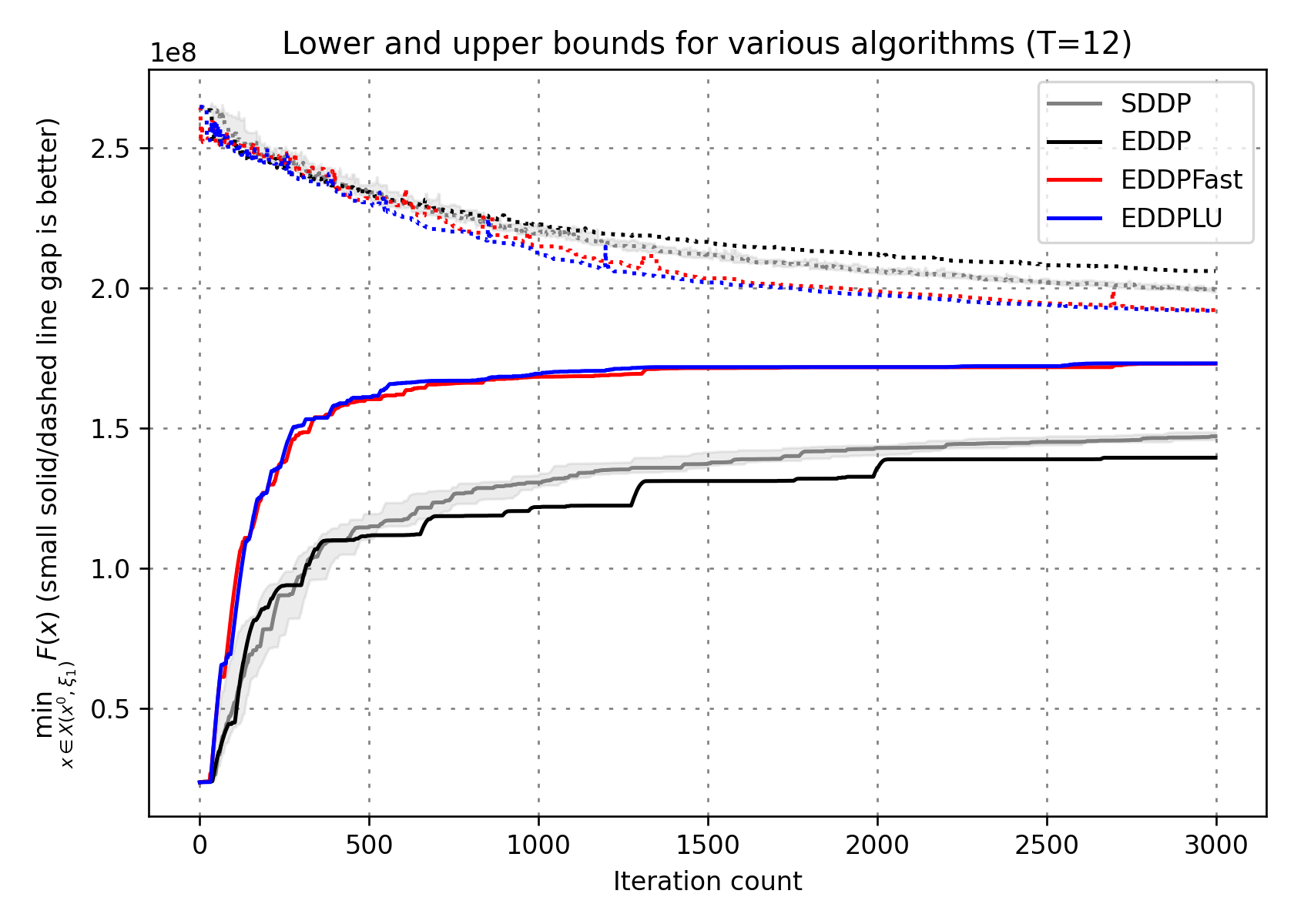
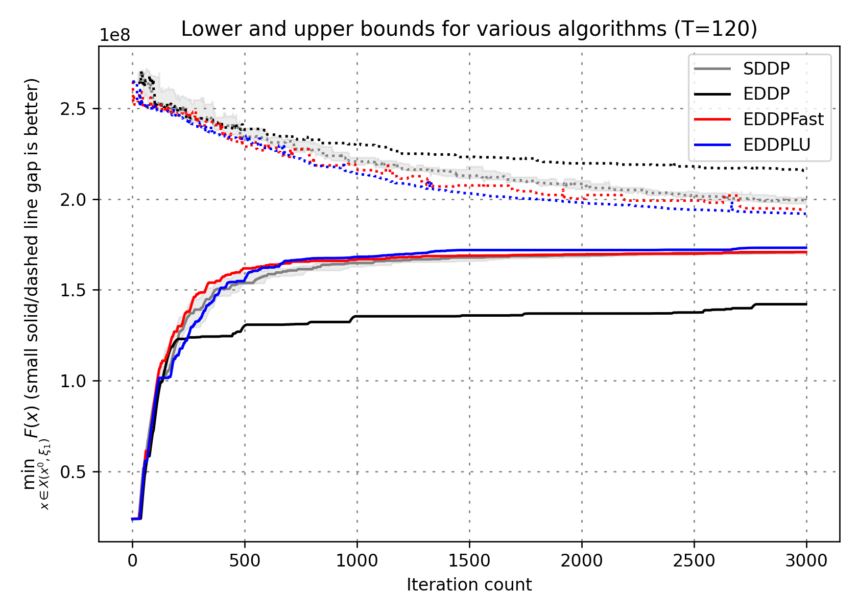
Figure 3: Upper and lower bounds for approximately solving $\min_{x\in X(x^{0},\xi_{1})}F(x)$, denoted by dashed and solid lines, respectively. We ran 10 trials of SDDP and plotted the 10th percentile, median, and 90th percentile performance at each iteration. The left and right figures show the bounds with an effective planning horizon of $T=12$ and $T=120$, respectively.

Now, we discuss our results in Figure 3. For $T=12$, both EDDPFast and EDDPLU produce tighter lower bounds and upper bounds than EDDP and SDDP. We also include plots of the lower and upper bounds as a function of wall clock time in Figure 4. Note that EDDPFast took 2584 seconds (approximately 0.75 hours) while EDDPLU took about 8.25 hours when run on a laptop with an Intel Core i5 at 2.3 GHz. This is because EDDPLU computes upper bounds for each search point. The runtime of SDDP is 2500 seconds when run on the same machine. This suggests the data structure $\mathcal{S}$ in EDDP, implemented as a dictionary, has a small computational overhead.

When $T=120$, SDDP matches the performance of EDDPFast despite its worse theoretical complexity (Theorem 4.6). One possible explanation is EDDPFast may be over-exploring the feasible region, while the random sampling of SDDP provides a more uniform coverage. One observation is that SDDP seems sensitive to the choice of $T$. A larger $T$ improves the lower bound performance, suggesting that resetting less often leads to better performance. This is the reason for our “no-reset” modification to EDDPFast and EDDPLU described earlier in this section. On the other hand, EDDPFast and EDDPLU seem to have similar performances for both $T$s.

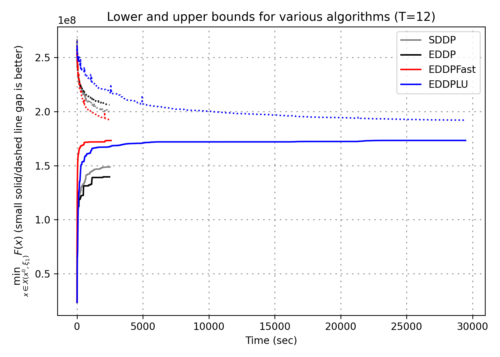
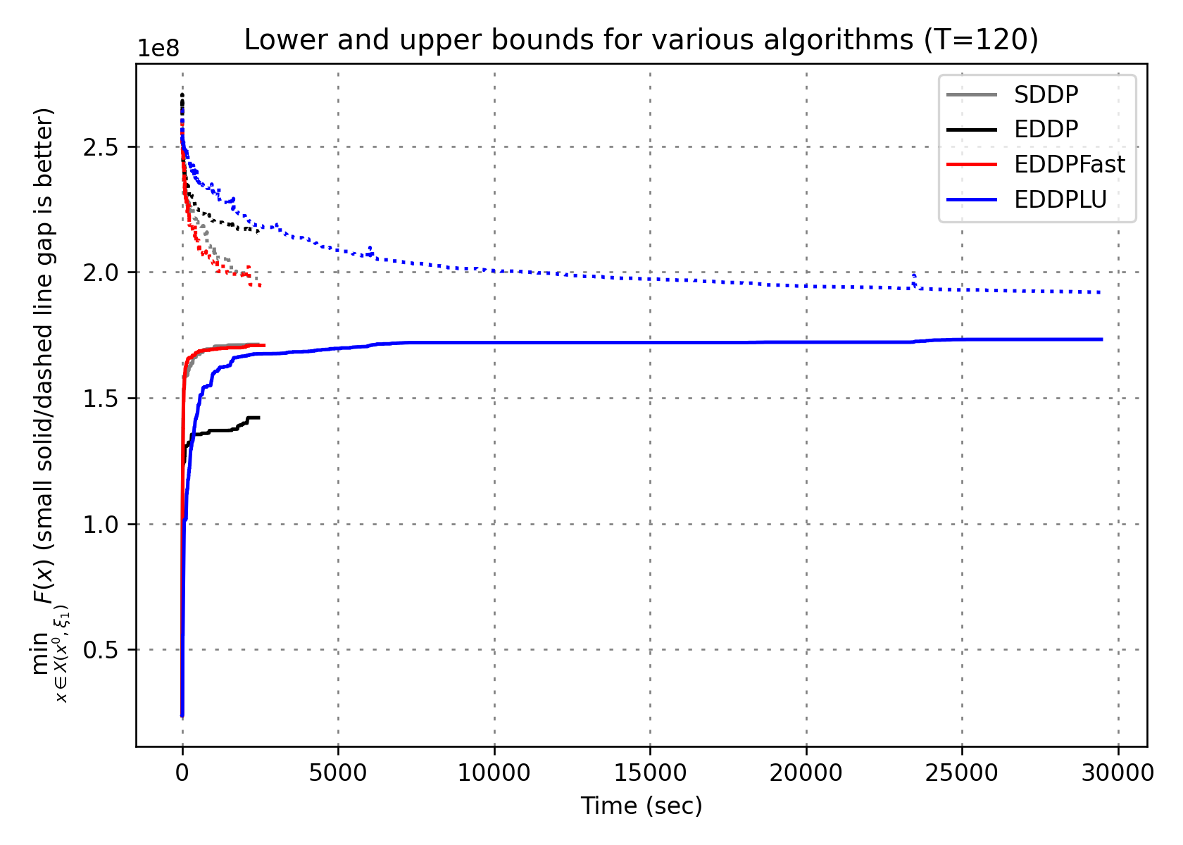
Figure 4: Upper and lower bound gaps as a function of time for various algorithms for $T=12$ and $T=120$ to run 3000 iterations. When plotting SDDP, we used the first trial’s data.

5.2 Convergence of hierarchical dual dynamic programming and inexact solvers

We consider solving a variation of the economic dispatch (ED) problem with linear costs. The objective is to satisfy the demands across $r$ regions using $n$ thermal power generators while minimizing the costs [36]. We modify ED in two ways. First, we introduce long-term energy storage, or batteries, that allow one to arbitrage energy prices by storing or using saved energy between different stages [36, 7]. Then, we take the optimal dual variables corresponding to the demand constraints as the cost coefficient for a second-stage ED problem with a single demand. The dual variables are also referred to as the marginal pricing or equilibrium price, and it is the price that ensures the market clears [35]. The resulting problem has the following interpretation: a grid operator wants to meet demand and minimize operating costs while ensuring electricity is cheap for an important service provider, such as a hospital. We set the number of scenarios in the SAA problems of the top-level and lower-level problems as $N_{1}=10$ and $N_{2}=10$, respectively. The discount factor is set to $\lambda=0.95$, the number of generators is set to $n=10$, and the number of demands in the first ED problem is set to $r=4$. Full details are in Appendix C.

We compare the setting where the subproblems are solved exactly in extensive form using an LP solver (i.e., Gurobi) and inexactly as a stochastic program using the primal-dual stochastic approximation (PDSA) method from Section 3.1. We refer to these methods as LP and PDSA, respectively. Since PDSA returns inexact subproblems, its cutting-plane model $\underline{V}^{k}$ can overestimate the cost-to-go function $V$ (c.f. Lemma 3.5). So we use the LP approach to evaluate both the lower and upper bounds of the solution returned by the LP and PDSA approach, as shown in Figure 5. We have that the lower bound values at iteration 150 for the LP and PDSA approach are 427039 and 427417, respectively. Their upper bounds are 429669 and 431389, respectively. Therefore, the relative error of the solution returned by PDSA is at most 1.02%.

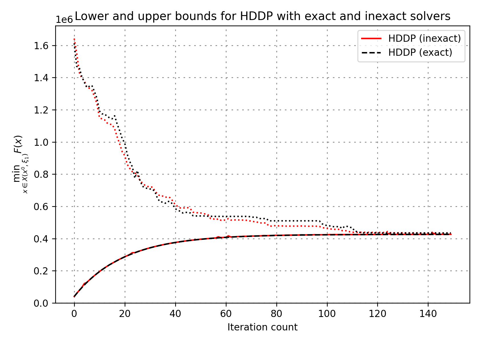
Figure 5: Upper and lower bounds for $\min_{x\in X(x^{0},\xi_{1})}F(x)$. We compared EDDP where the subproblem is a large-scale LP and solved exactly with Gurobi vs. a stochastic problem and solved inexactly via PDSA. Both upper and lower bounds were only evaluated using the models from the method with exact solutions.

5.3 Scalability of dual dynamic programming

We test the parallel performance of hierarchical dual dynamic programming for solving the modified economic dispatch problem from the previous Section 5.2. We use Python’s built-in multiprocessing library for shared-memory parallelism and ran on an Intel Xeon Gold 6226 CPU at 2.70GHz, which has 12 cores each with 2 threads, from Georgia Tech’s Phoenix compute cluster [21].

Our scaling results are shown in Figure 6. We start with $N=128$ scenarios and $n=100$ variables for the top-level problem and run PDSA for a fixed number of iterations. For our strong scaling results, we solve the same problem while increasing the number of solvers from $p=1,2,4,8,16$. We then measure the speedup, defined as the runtime with 1 solver vs the runtime with $p$ solvers, and compare it to the perfect speedup, which is the number of parallel solvers available. For weak scaling, we increase the number of scenarios at the same rate as the number of solvers, e.g., $p=4$ solvers for $N=512$ scenarios. We then measure the efficiency, which is the runtime with 1 solver divided by the runtime with $p$ solvers. The ideal efficiency is 1. Overall, we see both strong and weak scaling reach perfect speedup and ideal efficiency up to 8 processors. When we move to 16 processors, the performance degrades. One explanation is that the CPU has 12 cores, and so some of the solvers reside on the same core but on different threads, which may cause some slowdown.

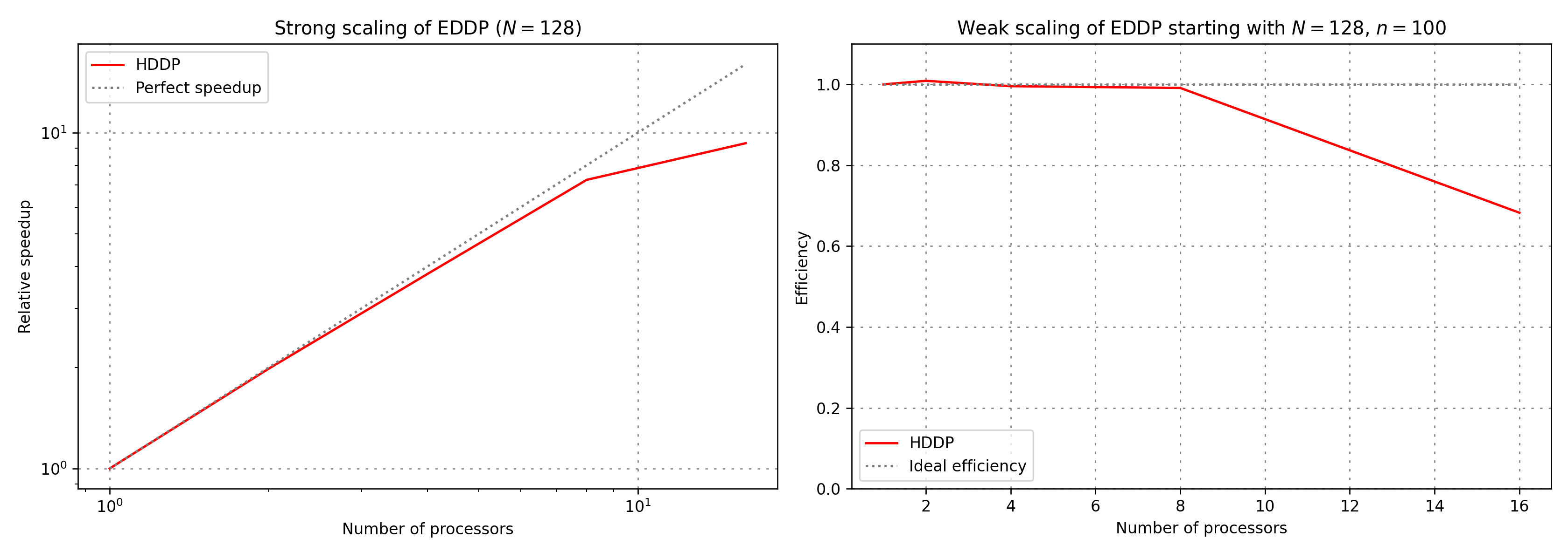
Figure 6: Strong and weak scaling of HDDP. All problems solve the hierarchical economic dispatch problem starting with $N=128$ scenarios and a top-level decision size of $n=100$ subproblems.

6 Conclusion

We show dual dynamic programming can solve stochastic programs over an infinite horizon, including a class of hierarchical stationary stochastic programs. Our theoretical results include a modification of explorative dual dynamic programming to reduce the dependence on the effective planning horizon and showing the dimension of the lower-level problem from a hierarchical problem does not explicitly affect the number of iterations. Both our theoretical and numerical results show that resetting, i.e., setting $x^{k-1}=x^{0}$ as the next search point, may slow the growth of the cutting-plane model, suggesting the selection of search points is crucial for a tighter cutting-plane model.

Appendix A Proof of Theorem 3.2

Recall the light-tail assumption in Eq. 29, which is satisfied in the finite-sum case when the subgradients are all bounded. Let us establish a corollary of this assumption.

Lemma A.1 (Lemma 4.1 [17]).

Let $\xi_{[t]}\equiv\left\{\xi_{1},\xi_{2},\ldots,\xi_{t}\right\}$ be a sequence of i.i.d. random variables, and $\zeta_{t}=\zeta_{t}(\xi_{[t]})$ be deterministic Borel functions of $\xi_{[t]}$ such that $\mathbb{E}_{\mid\xi_{[t-1]}}\left[\zeta_{t}\right]=0$ a.s. and $\mathbb{E}_{\mid\xi_{[t-1]}}\left[\exp\left\{\zeta_{t}^{2}/\sigma_{t}^{2}\right\}\right]\leq\exp\{1\}$ a.s., where $\sigma_{t}>0$ are deterministic. Then

$$\forall\lambda\geq 0:\operatorname{Pr}\left\{\sum_{t=1}^{N}\zeta_{t}>\lambda\sqrt{\sum_{t=1}^{N}\sigma_{t}^{2}}\right\}\leq\exp\left\{-\lambda^{2}/3\right\}$$

We also have the following result regarding the Q-gap function.

Proposition A.2 (Theorem 3 [19]).

Suppose the parameters of PDSA (Algorithm 3) satisfy the conditions Theorem 3.2. Then

$$Q\left(\bar{z}_{N},z\right)\leq\frac{1}{\sum_{k=1}^{N}w_{k}}\left(w_{1}\tau_{1}V_{X}\left(x_{0},x\right)+\frac{w_{1}\eta_{1}}{2}\left\|y_{0}-y\right\|^{2}-\frac{w_{N}\eta_{N}}{2}\left\|y_{N}-y\right\|^{2}+\sum_{k=1}^{N}\Lambda_{k}\right)$$ (43)

for any $z\in Z$, where

$$\Lambda_{k}:=w_{k}\left[\left(\overline{G}+\left\|G_{k-1}\right\|_{*}\right)^{2}/\left(\alpha_{X}\tau_{k}\right)+\left\langle\Delta_{k},x_{k-1}-x\right\rangle+\bar{\epsilon}\right].$$

We can now prove Theorem 3.2.

Proof of Theorem 3.2.

To prove (a), we fix $y=y_{*}$ in Eq. 43, recall the definition of $D_{X}$ implies $V(x_{0},x)\leq D_{X}$, and maximize Eq. 43 w.r.t. $x\in X$ (recall $\mathrm{gap}_{*}(\bar{z})=\max_{x\in X}Q(\bar{z};x,y_{*})$) to derive

$$\mathrm{gap}_{*}(\bar{z}_{N})\leq\big{(}\sum\limits_{k=1}^{N}w_{k}\big{)}^{-1}\big{[}w_{1}\tau_{1}D_{X}^{2}+\frac{w_{1}\eta_{1}}{2}\|y_{*}-y_{0}\|^{2}+\sum\limits_{k=1}^{N}\Lambda_{k}\big{]}.$$ (44)

We will now bound the gradient error terms $\Lambda_{k}$. We have

$$\begin{split}\sum\limits_{k=1}^{N}\Lambda_{k}&=\sum\limits_{k=1}^{N}\Big{(}\frac{(\overline{G}+\|G_{k-1}\|_{*})^{2}}{\tau_{k}\alpha_{X}}+\bar{\epsilon}+\langle\Delta_{k-1},x_{k-1}-x_{k-1}^{v}\rangle+\langle\Delta_{k-1},x_{k-1}^{v}-x\rangle\Big{)}\\ &\leq\sum\limits_{k=1}^{N}w_{k}\Big{(}\frac{4\overline{G}^{2}}{\alpha_{X}\tau_{k}}+\bar{\epsilon}+\langle\Delta_{k-1},x_{k-1}-x_{k-1}^{v}\rangle\Big{)}+w_{1}\tau_{1}D_{X}^{2}+\sum\limits_{k=1}^{N}\frac{w_{k}\|\Delta_{k-1}\|^{2}}{2\alpha_{X}\tau_{k}},\end{split}$$ (45)

where the inequality is by $\|G_{k-1}\|\leq\overline{G}$ and [19, Lemma 4]. Now, let us define $\varsigma_{k}=w_{k}\langle\Delta_{k-1},x_{k-1}-x_{k-1}^{v}\rangle$, which forms a martingale-difference sequence. Then

$$\mathbb{E}_{|\xi_{[k-1]}}[\mathrm{exp}\{\varsigma_{k}^{2}/(w_{k}D_{X}\sigma)^{2}\}] \leq\mathbb{E}_{|\xi_{[k-1]}}[\mathrm{exp}\{\|\Delta_{k-1}\|_{*}^{2}\|x_{k-1}-x^{v}_{k-1}\|^{2}/(D_{X}\sigma)^{2}\}]$$

$$\leq\mathbb{E}_{|\xi_{[k-1]}}[\mathrm{exp}\{\|\Delta_{k-1}\|_{*}^{2}/\sigma^{2}\}]$$

$$\leq\mathrm{exp}\{1\},$$

where the last line is by the “light-tail” assumption (Eq. 29). Now, applying the previous Lemma A.1 with $\zeta_{k}=\varsigma_{k}$ and $\sigma_{k}=w_{k}D_{X}\sigma$, we get

$$\mathrm{Pr}\Big{\{}\sum\limits_{k=1}^{N}\underbrace{w_{k}\langle\Delta_{k-1},x_{k-1}-x_{k-1}^{v}\rangle}_{\varsigma_{k}}>\lambda D_{X}\sigma\sqrt{\sum\limits_{k=1}^{N}w_{k}^{2}}\Big{\}} \leq\mathrm{exp}\{-\lambda^{2}/3\}.$$ (46)

Now, define the constants $\theta_{k}=\beta_{k}/(\sum\limits_{t=1}^{N}\beta_{t})$ and $\beta_{k}=w_{k}/(2\alpha_{X}\tau_{k})$. By Jensen’s inequality, $\mathrm{exp}\big{\{}\sum\limits_{k=1}^{N}\theta_{k}(\|\Delta_{k-1}\|_{*}^{2}/\sigma^{2})\big{\}}\leq\sum\limits_{k=1}^{N}\theta_{k}\mathrm{exp}\{\|\Delta_{k-1}\|_{*}^{2}/\sigma^{2}\}$. Then by recalling $\theta_{k}$, taking expectations, and using the “light-tail” assumption, we get

$$\mathbb{E}\Big{[}\mathrm{exp}\big{\{}\sum\limits_{k=1}^{N}\beta_{k}\|\Delta_{k-1}\|_{*}^{2}/\big{(}\sum\limits_{t=1}^{N}\beta_{t}\sigma^{2}\big{)}\big{\}}\Big{]}\leq\sum\limits_{k=1}^{N}\theta_{k}\mathbb{E}[\mathrm{exp}\{\|\Delta_{k-1}\|_{*}^{2}/\sigma^{2}\}]\leq\mathrm{exp}\{1\}.$$

By Markov’s inequality, we can conclude for any $\lambda\geq 0$,

$$\begin{split}\mathrm{Pr}&\big{\{}\sum\limits_{k=1}^{N}\beta_{k}\|\Delta_{k-1}\|_{*}^{2}>(1+\lambda)\sigma^{2}\sum\limits_{k=1}^{N}\beta_{k}\big{\}}\\ &=\mathrm{Pr}\Big{\{}\mathrm{exp}\big{(}\sum\limits_{k=1}^{N}\beta_{k}\|\Delta_{k-1}\|_{*}^{2}/(\sum\limits_{t=1}^{N}\beta_{t}\sigma^{2})\big{)}>\mathrm{exp}(1+\lambda)\Big{\}}\leq\mathrm{exp}\{-\lambda\}.\end{split}$$ (47)

By combining Eq. 45, Eq. 46, and Eq. 47 with union bound and recalling the definition of $C_{k}(\lambda)$ in Eq. 31, we guarantee,

$$\begin{split}\mathrm{Pr}&\bigg{\{}\sum\limits_{k=1}^{N}\Lambda_{k}>w_{1}\tau_{1}D_{X}^{2}+\lambda D_{X}\sigma\sqrt{\sum\limits_{k=1}^{N}w_{k}^{2}}+\sum\limits_{k=1}^{N}w_{k}\Big{(}\frac{4\overline{G}^{2}+(1+\lambda)\sigma^{2}}{\alpha_{X}\tau_{k}}+\bar{\epsilon}\Big{)}\bigg{\}}\\ &=\mathrm{Pr}\Big{\{}\sum\limits_{k=1}^{N}\Lambda_{k}>w_{1}\tau_{1}D_{X}^{2}+C_{N}(\lambda)+\bar{\epsilon}\big{(}\sum\limits_{k=1}^{N}w_{k}\big{)}\Big{\}}\\ &\leq\mathrm{exp}\{-\lambda\}+\mathrm{exp}\{-\lambda^{2}/3\}.\end{split}$$ (48)

Substituting this bound in Eq. 44 and noticing the parameters and $\|y^{*}-y_{0}\|$ are deterministic leads us to the following bound, which holds with probability at least $1-(\mathrm{exp}\{-\lambda\}+\mathrm{exp}\{-\lambda^{2}/3\})$,

$$\mathrm{gap}_{*}(\bar{z}_{N}) \leq\big{(}\sum\limits_{k=1}^{N}w_{k}\big{)}^{-1}\Big{[}2w_{1}\tau_{1}D_{X}^{2}+\frac{w_{1}\eta_{1}}{2}\|y_{*}-y_{0}\|^{2}+C_{N}(\lambda)\Big{]}+\bar{\epsilon}.$$

We now show part (b). Adding $\langle\delta,y\rangle$ to both sides of Eq. 43 and using the fact $w_{1}\eta_{1}=w_{N}\eta_{N}$, we have

$$Q(\bar{z}_{N},z)+\langle\delta,y\rangle$$

$$\leq\big{(}\sum\limits_{k=1}^{N}w_{k}\big{)}^{-1}\Big{[}w_{1}\tau_{1}V(x_{0},x)+w_{1}\eta_{1}\big{(}\frac{\|y_{0}-y\|^{2}}{2}-\frac{\|y_{N}-y\|^{2}}{2}+\langle y_{0}-y_{N},y\rangle\big{)}+\sum\limits_{k=1}^{N}\Lambda_{k}\Big{]}$$

$$\leq\big{(}\sum\limits_{k=1}^{N}w_{k}\big{)}^{-1}\Big{[}w_{1}\tau_{1}D_{X}^{2}+\frac{w_{1}\eta_{1}}{2}\|y_{0}\|^{2}+\sum\limits_{k=1}^{N}\Lambda_{k}\Big{]}.$$

Maximizing with respect to $(x,y)\in X\times K_{*}$ and using our high probability bound Eq. 48, we ensure that with probability a least $1-(\mathrm{exp}\{-\lambda\}+\mathrm{exp}\{-\lambda^{2}/3\})$ (i.e., the same event space that gave us our bound on $\mathrm{gap}_{*}(\bar{z}_{N})$),

$$\mathrm{gap}_{\delta}(\bar{z}_{N}) \leq\big{(}\sum\limits_{k=1}^{N}w_{k}\big{)}^{-1}\Big{[}2w_{1}\tau_{1}D_{X}^{2}+\frac{w_{1}\eta_{1}}{2}\|y_{0}\|^{2}+C_{N}(\lambda)\Big{]}+\bar{\epsilon}.$$

It remains to bound $\|\delta\|$. Fixing $x=x_{*}$ in Eq. 43 (and recalling $V(x_{0},x)\leq D_{X}^{2}$) and using the fact $Q(\bar{z}_{N},[x_{*},y_{*}])\geq 0$ by definition of the saddle point, we have

$$\frac{w_{N}\eta_{N}}{2}\|y_{*}-y_{N}\|^{2}\leq w_{1}\tau_{1}D_{X}^{2}+\frac{w_{1}\eta_{1}}{2}\|y_{*}-y_{0}\|^{2}+\sum\limits_{k=1}^{N}\Lambda_{k}.$$

Using the high-probability bound Eq. 48 and assumption $w_{1}\eta_{1}=w_{N}\eta_{N}$, the above implies with probability $1-(\mathrm{exp}\{-\lambda\}+\mathrm{exp}\{-\lambda^{2}/3\})$,

$$\begin{split}\frac{w_{N}\eta_{N}}{2}\|y_{N}-y^{*}\|^{2}&\leq 2w_{1}\tau_{1}D_{X}+\frac{w_{1}\eta_{1}}{2}\|y_{0}-y^{*}\|+C_{N}(\lambda)+\bar{\epsilon}\big{(}\sum\limits_{k=1}^{n}w_{k}\big{)},\end{split}$$ (49)

which in view of $w_{1}\eta_{1}=w_{N}\eta_{N}$ and subadditivity of square root leads us to

$$\|y_{N}-y^{*}\| \leq 2\sqrt{\frac{\tau_{1}}{\eta_{1}}}D_{X}+\|y_{0}-y^{*}\|+\sqrt{\frac{2}{w_{1}\eta_{1}}\Big{(}C_{N}(\lambda)+\bar{\epsilon}\big{(}\sum\limits_{k=1}^{N}w_{k}\big{)}\Big{)}}.$$

The above inequality and relation $\|\delta\|\leq(\sum\limits_{k=1}^{N}w_{k})^{-1}[w_{1}\eta_{1}(\|y_{0}-y^{*}\|+\|y^{*}-y_{N}\|)]$ yields

$$\|\delta\| \leq\frac{w_{1}\eta_{1}}{\sum\nolimits_{k=1}^{N}w_{k}}\Big{[}2\sqrt{\frac{\tau_{1}}{\eta_{1}}}D_{X}+2\|y_{0}-y^{*}\|+\sqrt{\frac{2}{w_{1}\eta_{1}}\Big{(}C_{N}(\lambda)+\bar{\epsilon}\big{(}\sum\limits_{k=1}^{N}w_{k}\big{)}\Big{)}}\Big{]}.$$

∎

Appendix B The no-reset modification to EDDP

This section provides the details of the no-reset modification introduced in Section 5.1. We modify the definition of the next search point $x^{k}$ and introduce a new set of search points as follows. Starting with $x^{0}=x^{0}_{\text{nr}}$, we define for $k\geq 1$,

$$x^{k} =\mathrm{argmax}_{x\in\{x_{0}^{k}\}\cup\{x^{k}_{i,\text{nr}}\}_{i=1}^{N}}\mathcal{S}(x)$$ (50)

$$x^{k}_{\text{nr}} =\mathrm{argmax}_{x\in\{x^{k}_{i,\text{nr}}\}_{i=1}^{N}}\mathcal{S}(x),$$

where

$$x^{k}_{i} \in\mathrm{argmin}_{x\in\scriptsize\begin{cases}X(x^{0},\tilde{\xi}_{i}):i=0\\ X(x^{k-1},\tilde{\xi}_{i}):i\geq 1\end{cases}}\left\{\underline{F}^{k}_{i}(x):=h(x,\tilde{c}_{i})+\lambda\underline{V}^{k-1}(x)\right\},\ \forall 0\leq i\leq N$$

$$x^{k}_{i,\text{nr}} \in\mathrm{argmin}_{x\in X(x^{k-1}_{\text{nr}},\tilde{\xi}_{i})}\left\{\underline{F}^{k}_{i}(x):=h(x,\tilde{c}_{i})+\lambda\underline{V}^{k-1}(x)\right\},\ \forall 1\leq i\leq N.$$

Here, “nr” stands for “no-reset.” The definition of $x^{k}_{i}$ is identical to the one in modified EDDP (c.f. Eq. 22). The main difference is in the definition of the next search point $x^{k}$, which relies on the “no-reset” search points $x^{k}_{i,\text{nr}}$. The previous “no-reset” search point, $x^{k-1}_{\text{nr}}$, is used instead of $x^{k-1}$ as the previous search point when obtaining $x^{k}_{i,\text{nr}}$. As the name suggests, we never set $x^{k}_{\text{nr}}=x^{k}_{0}$ explicitly, where $x^{k}_{0}$ is the solution to the zeroth index subproblem. We use these new search points $x^{k}_{i,\text{nr}}$ to define $x^{k}$, where instead of choosing from $\{x^{k}_{i}\}_{i=0}^{N}$ (c.f. Eq. 23), we choose from the union of $x^{k}_{0}$ and $\{x^{k}_{i,\text{nr}}\}_{i=1}^{N}$. Everything else in the modified EDDP remains unchanged. The motivation for this modification is to not set the previous search point as the initial state variable, $x^{0}$. This is because empirically, we found that choosing the previous search point as $x^{0}$ limited the growth to $\underline{V}^{k}$. One can check the modified EDDP maintains the same theoretical guarantees as long as $x^{k}\in\mathrm{argmax}_{x\in X^{\prime}}\mathcal{S}(x)$, where $X^{\prime}\subseteq\mathcal{X}$ is an arbitrary set that includes $x^{k}_{0}$ (c.f. Eq. 50).

Appendix C Economic dispatch with batteries and marginal pricing

We consider the following variation of economic dispatch (ED) [35, 36]. The basic ED problem consists of $n$ generators where generator $i$ has cost $c_{i}$ to generate one unit of power. Generators $i\in I_{k}$ must collectively generate power to satisfy the demand at region $k$, $\tilde{d}_{k}$, while respecting lower and upper bounds of $\underline{g}$ and $\overline{g}$, respectively. The set $I_{k}$ is a subset of $\{1,\ldots,n\}$. The tilde indicates this is a random variable, and we assume there are $r$ regions in total. We add long-term energy storage, or a battery, at each region. Let $b_{r}^{(t)}$ and $b_{r}^{(t+1)}$ be the power stored in the battery at region $r$ at the beginning of time $t$ and $t+1$, respectively. We assume the current battery level $b^{(t)}_{k}$ is given, and the battery levels must lie within $[\underline{b},\overline{b}]$. In addition to meeting demand, the generators can store excess power or borrow energy from the batteries. We multiply $b_{i}^{(t)}$ by a constant $\beta\in(0,1]$ (in our experiments, we randomly sampled $\beta$ from between $[0.8,1]$) to indicate energy loss from battery storage/transfer. The resulting linear program (LP) is

$$P(c,\tilde{d}):=\min_{g,b^{(t+1)}}\ \sum\limits_{i=1}^{n}c_{i}\cdot g_{i}$$

s.t. $$\sum\limits_{i\in I_{k}}g_{i}+\beta\cdot b_{k}^{(t)}-b_{k}^{(t+1)}=\tilde{d}_{k},\ \forall k=1,\ldots,r$$ (51)

$$\underline{g}\leq g_{i}\leq\bar{g},\ \forall i=1,\ldots,n$$

$$\underline{b}\leq b_{k}^{(t+1)}\leq\bar{b},\ \forall k.$$

Assuming the LP is feasible, the optimal solution equals the dual LP,

$$\max_{p,u,v,y,z}\ \sum\limits_{k=1}^{r}(\tilde{d}_{k}-\beta\cdot b_{k}^{(t)})\cdot p_{k}+\underline{b}\cdot y_{k}-\overline{b}\cdot z_{k}+\sum\limits_{i=1}^{n}\underline{g}\cdot u_{i}-\overline{g}\cdot v_{i}$$

s.t. $$\sum\limits_{k:i\in I_{k}}p_{k}+(u_{i}-v_{i})=c_{i},\ \forall i=1,\ldots,n$$

$$-p_{k}+(y_{k}-z_{k})=0,\ \forall k=1,\ldots,r$$

$$u_{i},v_{i},y_{k},z_{k}\geq 0,\ \forall i,k.$$

The dual variable $p$ corresponding to the demand constraint (Eq. 51) is referred to as the shadow price or marginal pricing [35, 36]. The optimal dual value $p_{k}$ corresponds to the change in the objective of the primal for one additional unit of demand at region $k$. The dual variables $u$, $v$, $y$, and $z$ correspond to the various lower and upper bounds of the generators and batteries.

To make this a two-stage stochastic linear program, we consider solving

$$\max_{p,u,v,y,z}\{Q(p,u,v,y,z;b^{(t)})+\mathbb{E}[P(p,\tilde{D})]:(p,u,v,y,z)\in X_{\text{dual}}\},$$

where $Q(p,u,v,y,z;b^{(t)})$ and $X_{\text{dual}}$ are, respectively, the linear cost function (parameterized by $b^{(t)}$) and feasible region of the dual LP. We refer to $P(p,\tilde{D})$ as the second-stage problem, which is an ED problem with only one demand and $k$ generators, where the cost of generator $k$ is $p_{k}$. In the second-stage problem, we also include an extra generator to ensure the primal is always feasible. This additional generator’s cost is set to a large constant $C>0$ (independent of $p$) to discourage its use. The expectation is taken w.r.t. to the demand $\tilde{D}>0$. We approximate the expectation with an empirical average and rewrite the SAA problem as a linear program by writing the dual of the second-stage problem to de-couple the dual variable $p$ from the first-stage problem and generator variable $g$ from the second-stage problem. This results in a large “max” LP. Taking its dual results in the new primal LP,

$$\min_{g,b^{(t+1)},\{h^{\ell}\}_{\ell=1}^{N}}\ \sum\limits_{i=1}^{n}c_{i}\cdot g_{i}+\frac{1}{N}\sum\limits_{\ell=1}^{N}v_{2\ell}(\{h_{k}^{\ell}\}_{k})$$

s.t. $$\sum\limits_{i\in I_{k}}g_{i}+\beta\cdot b_{i}^{(t)}-b_{i}^{(t+1)}-\sum\limits_{\ell=1}^{N}h_{k}^{\ell}=\tilde{d}_{r},\ \forall k=1,\ldots,r$$

$$\underline{g}\leq g_{i}\leq\bar{g},\ \forall i=1,\ldots,n$$

$$\underline{b}\leq b_{k}\leq\bar{b},\ \forall k$$

$$\underline{h}\leq h_{k}^{\ell}\leq\overline{h},\ \forall k,\ell=1,\ldots,N,$$

where the second-stage problem is now the piecewise linear function

$$v_{2\ell}(\{h_{k}^{\ell}\}_{k}) :=\min\{C\cdot f:f\geq|\tilde{D}^{\ell}-(h_{1}^{\ell}+\sum\limits_{k=2}^{r}\alpha_{j}\cdot h_{k}^{\ell})|\}$$

$$=C\cdot|\tilde{D}^{\ell}-(h_{i}^{\ell}+\sum\limits_{k=2}^{r}\alpha\cdot h_{k}^{\ell})|.$$

Here, the variables $h_{k}^{\ell}$ correspond to the generator $k$ for scenario $\ell$ in the second-stage problem with bounds in $[\underline{h},\overline{h}]$. Meanwhile, $\alpha\in(0,1]$ (also sampled from $[0.8,1]$) is the loss of power for transferring power from generators $k=2,\ldots,r$ to meet the single demand. The constant $\tilde{D}^{\ell}$ is scenario $\ell$’s demand for the second-stage problem.

References

• Baucke [2018] R. Baucke. An algorithm for solving infinite horizon markov dynamic programmes. Optimization, 2018.
• Baucke et al. [2017] R. Baucke, A. Downward, and G. Zakeri. A deterministic algorithm for solving multistage stochastic programming problems. Optimization Online, page 25, 2017.
• Bellman [2010] R. E. Bellman. Dynamic programming. Princeton university press, 2010.
• Ben-Tal and Nemirovski [2001] A. Ben-Tal and A. Nemirovski. Lectures on modern convex optimization: analysis, algorithms, and engineering applications. SIAM, 2001.
• Bertsekas and Shreve [1996] D. P. Bertsekas and S. E. Shreve. Stochastic optimal control: the discrete-time case, volume 5. Athena Scientific, 1996.
• Birge [1985] J. R. Birge. Decomposition and partitioning methods for multistage stochastic linear programs. Operations research, 33(5):989–1007, 1985.
• Cole et al. [2017] W. Cole, B. Frew, T. Mai, Y. Sun, J. Bistline, G. Blanford, D. Young, C. Marcy, C. Namovicz, R. Edelman, et al. Variable renewable energy in long-term planning models: a multi-model perspective. Technical report, National Renewable Energy Lab.(NREL), Golden, CO (United States), 2017.
• Ding et al. [2019] L. Ding, S. Ahmed, and A. Shapiro. A python package for multi-stage stochastic programming. Optimization online, pages 1–41, 2019.
• Fullner and Rebennack [2021] C. Fullner and S. Rebennack. Stochastic dual dynamic programming and its variants. Karlsruhe Institude of Technology, 2021.
• Grinold [1986] R. C. Grinold. Infinite horizon stochastic programs. SIAM journal on control and optimization, 24(6):1246–1260, 1986.
• Guigues [2016] V. Guigues. Convergence analysis of sampling-based decomposition methods for risk-averse multistage stochastic convex programs. SIAM Journal on Optimization, 26(4):2468–2494, 2016.
• Guigues [2020] V. Guigues. Inexact cuts in stochastic dual dynamic programming. SIAM Journal on Optimization, 30(1):407–438, 2020.
• Jiang et al. [2015] N. Jiang, A. Kulesza, S. Singh, and R. Lewis. The dependence of effective planning horizon on model accuracy. In Proceedings of the 2015 International Conference on Autonomous Agents and Multiagent Systems, pages 1181–1189, 2015.
• [14] J. E. Kelley, Jr. The cutting-plane method for solving convex programs. Journal of the society for Industrial and Applied Mathematics, 8(4).
• Kleywegt et al. [2002] A. J. Kleywegt, A. Shapiro, and T. Homem-de Mello. The sample average approximation method for stochastic discrete optimization. SIAM Journal on Optimization, 12(2):479–502, 2002.
• Lan [2020a] G. Lan. Complexity of stochastic dual dynamic programming. Mathematical Programming, pages 1–38, 2020a.
• Lan [2020b] G. Lan. First-order and stochastic optimization methods for machine learning, volume 1. Springer, 2020b.
• Lan and Zhou [2018] G. Lan and Y. Zhou. An optimal randomized incremental gradient method. Mathematical programming, 171:167–215, 2018.
• Lan and Zhou [2021] G. Lan and Z. Zhou. Dynamic stochastic approximation for multi-stage stochastic optimization. Mathematical Programming, 187(1):487–532, 2021.
• Nannicini et al. [2021] G. Nannicini, E. Traversi, and R. W. Calvo. A Benders squared (B2) framework for infinite-horizon stochastic linear programs. Mathematical Programming Computation, 13(4):645–681, 2021.
• PACE [2017] PACE. Partnership for an Advanced Computing Environment (PACE), 2017. URL http://www.pace.gatech.edu.
• Pereira and Pinto [1991] M. V. Pereira and L. M. Pinto. Multi-stage stochastic optimization applied to energy planning. Mathematical programming, 52(1):359–375, 1991.
• Pflug and Pichler [2014] G. C. Pflug and A. Pichler. Multistage stochastic optimization, volume 1104. Springer, 2014.
• Philpott and Guan [2008] A. B. Philpott and Z. Guan. On the convergence of stochastic dual dynamic programming and related methods. Operations Research Letters, 36(4):450–455, 2008.
• Powell [2007] W. B. Powell. Approximate Dynamic Programming: Solving the curses of dimensionality, volume 703. John Wiley & Sons, 2007.
• Rockafellar [1970] R. T. Rockafellar. Convex analysis, volume 18. Princeton university press, 1970.
• Shalev-Shwartz et al. [2012] S. Shalev-Shwartz et al. Online learning and online convex optimization. Foundations and Trends® in Machine Learning, 4(2):107–194, 2012.
• Shapiro [2011] A. Shapiro. Analysis of stochastic dual dynamic programming method. European Journal of Operational Research, 209(1):63–72, 2011.
• Shapiro and Cheng [2021] A. Shapiro and Y. Cheng. Central limit theorem and sample complexity of stationary stochastic programs. Operations Research Letters, 49(5):676–681, 2021.
• Shapiro and Cheng [2022] A. Shapiro and Y. Cheng. Dual bounds for periodical stochastic programs. Operations Research, 2022.
• Shapiro and Ding [2020] A. Shapiro and L. Ding. Periodical multistage stochastic programs. SIAM Journal on Optimization, 30(3):2083–2102, 2020.
• Shapiro and Nemirovski [2005] A. Shapiro and A. Nemirovski. On complexity of stochastic programming problems. In Continuous optimization, pages 111–146. Springer, 2005.
• Shapiro et al. [2021] A. Shapiro, D. Dentcheva, and A. Ruszczynski. Lectures on stochastic programming: modeling and theory. SIAM, 2021.
• Siddig et al. [2021] M. Siddig, Y. Song, and A. Khademi. Rolling horizon policies in multistage stochastic programming. arXiv preprint arXiv:2102.04874, 2021.
• Stevens [2016] N. Stevens. Models and algorithms for pricing electricity in unit commitment. PhD thesis, Master’s thesis, 2016.
• Wood et al. [2013] A. J. Wood, B. F. Wollenberg, and G. B. Sheblé. Power generation, operation, and control. John Wiley & Sons, 2013.
• Zhang and Sun [2022a] S. Zhang and X. A. Sun. On distributionally robust multistage convex optimization: Data-driven models and performance. arXiv preprint arXiv:2210.08433, 2022a.
• Zhang and Sun [2022b] S. Zhang and X. A. Sun. Stochastic dual dynamic programming for multistage stochastic mixed-integer nonlinear optimization. Mathematical Programming, pages 1–51, 2022b.