Efficient Aberration Correction via Optimal Bulk Speed of Sound Compensation

Abstract

Diagnostic ultrasound is a versatile and practical tool in the abdomen, and is particularly vital toward the detection and mitigation of early-stage non-alcoholic fatty liver disease (NAFLD). However, its performance in those with obesity—who are at increased risk for NAFLD—is degraded due to distortions of the ultrasound as it traverses thicker, acoustically heterogeneous body walls (aberration). Extant aberration correction methods for ultrasound are typically computationally intensive, as they require analysis of the much larger time series dataset, while optimizations based on image quality have not been analyzed or tested in the case of abdominal aberration. Herein, we assess analytically the capability of a single, optimal bulk speed of sound correction in receive beamforming to correct aberration, and improve the resulting images. Additionally, we propose an objective metric on the beamformed image to identify this speed of sound. We find that a bulk correction may approximate the aberration profile for layers or relevant thicknesses (1 to 3 cm) and speeds of sound (1400 to 1500 m/s). Additionally, through in vitro experiments, we show significant improvement in resolution (average point target width reduced by $60\text{\,}\mathrm{\char 37\relax}$) and improved boundary delineation in vivo with bulk speed of sound correction determined automatically from the beamformed images. Together, our results demonstrate the utility of simple, efficient bulk speed of sound correction to improve the quality of diagnostic liver images.

Keywords Ultrasound  $\cdot$ Aberration  $\cdot$ NAFLD

1 Introduction

Diagnostic ultrasound (US) is a versatile and practical tool in the abdomen, and has found widespread use cases including trauma assessment,¹ vascular imaging, ² and even detection of appendicitis.³ Of particular interest is its extension to the detection and mitigation of early-stage NAFLD, ^{4; 5} which presents a large and ever-growing public health challenge.^{6; 7} Ultrasound is affordable, safe, and portable compared to other modalities such as MRI or CT ⁴, with comparable diagnostic ability (up to order $85\text{\,}\mathrm{\char 37\relax}$ sensitivity and $95\text{\,}\mathrm{\char 37\relax}$ specificity.⁸) However, the risk of NAFLD is elevated among those with obesity ^{9; 10; 11} and these are patients for whom US imaging is degraded.^{12; 13} Thus, there is a pressing need for practicable methods for improving the quality and utility of abdominal US images among this group.

Nearly all commercial US imaging systems employ some form of conventional delay-and-sum (DAS) algorithms, which can provide effectively real-time imaging (ca. 30 frames per second), but inherently assume that speed of sound (SoS) is constant throughout the medium (typically $1540\text{\,}\mathrm{m}\mathrm{/}\mathrm{s}$ for abdominal applications). However, as the wavefront propagates through thick subcutaneous fat layers (SoS $\approx$ $1450\text{\,}\mathrm{m}\mathrm{/}\mathrm{s}$¹⁴), or indeed any heterogeneity in the speed of sound field, they are distorted such that delays appropriate for a SoS of $1540\text{\,}\mathrm{m}\mathrm{/}\mathrm{s}$ no longer result in constructive interference of the signals, and thus the image quality is degraded. This effect is termed “aberration”, and is the primary source of image degradation.¹⁵

Several techniques have been proposed to correct ultrasound aberration. Some techniques correlate individual channels with adjacent channels or their beamsum^{16; 17} to correct for shifts introduced by an aberrating medium (termed the aberration profile). Other techniques model aberration as contributions from off-axis scatterers, whose influence may be compensated for to reduce their effects.^{18; 19} Recent work has proposed methods to infer aberration profiles directly from the channel²⁰ or image²¹ data. Other methods look to simulate or measure an effective generated point source^{22; 23} in the medium such that the aberration profile may be deduced and applied to each channel. Corrections may also be computed from a known SoS distribution,²⁴ though obtaining these distributions from ultrasound data is nontrivial.^{25; 26; 27} Recent image formation methods have proposed alternative beamforming techniques to suppress clutter^{28; 29; 30} or find optimal channel weightings³¹ to mitigate incoherent contributions to the final image, though these methods often demonstrate lower inherent resolution compared to DAS in the case of low to moderate noise.³²

Additionally, several groups have investigated the use of a constant SoS that is different from $1540\text{\,}\mathrm{m}\mathrm{/}\mathrm{s}$ in the beamforming to improve the resulting images, including organ-specific values ³³. Anderson and Trahey³⁴ proposed using a quadratic least squares fit to the received echoes, though this method is limited to linear arrays. Other approaches seek the SoS that maximizes the coherence across the array,³⁵ or to maximize beamformed signal’s amplitude,^{36; 37} minimizes its phase variation,³⁸ or both;³⁹ however, these methods all rely on metrics computed from the channel data. Napolitano et al. proposed a spatial frequency metric to identify the optimal speed of sound from the resulting images themselves,⁴⁰ which was shown to agree the intensity-based metric; however, this work considered only lateral spatial frequencies, and thus has inherently limited sensitivity to features that vary in the axial direction.

While per-channel AC schemes have demonstrated improved imaging, nearly all require analysis and subsequent manipulation of the channel data, which imposes a significant computational burden, and requires access to the raw signals (rather than the beamformer output) directly. Altering the bulk SoS has demonstrated improved imaging results, but such techniques have largely been posited for material characterization, require full channel data analysis, or may degrade with aberration.^{34; 41; 37} Given the effectively real-time nature ultrasound systems, and computational constraints relative to emerging point of care devices, an efficient image-based method use would provide clear and immediate clinical benefit. Here, we propose such an efficient aberration correction scheme that identifies an optimal SoS for DAS beamforming from the beamformed images, establish theoretical bounds on its applicability and effectiveness, and show through in vitro and in vivo experiments that it may achieve nearly $40\text{\,}\mathrm{\char 37\relax}$ improvement in resolution with little added computational complexity.

2 Materials and Methods

The efficacy of a single, optimal SoS depends on the geometry and acoustic properties of the imaging arrangement. Given the interest here in abdominal imaging, for which a subcutaneous fat layer is the primary source of aberration, we will consider a layered geometry and examine the theoretical validity of $c_{\mathrm{opt}}$, as well as its experimental recovery and efficacy.

2.1 Bulk Speed of Sound Correction Validity

To establish limits on the ability of a single SoS to approximate an aberration profile for a given geometry (Fig. 1), we first considered an analytical approach. The appropriate receive delay corresponding to the time-of-flight between each transducer element and each point in the image is governed by propagation effects whose impact is determined by the physical properties and distribution of the medium. This analysis contains several inherent assumptions, which are first considered.

2.1.1 Geometric Acoustics Assumption

First, a geometric model of acoustic propagation (i.e., ray model) requires that the amplitude and direction of the wave vary slowly compared with the acoustic wavelength; this is reasonable for the case of abdominal ultrasound where $\lambda\sim$500\text{\,}\mathrm{\SIUnitSymbolMicro m}$$ and anatomical features of interest have scale of tens of millimeters. Second, ultrasound in general will be refracted as it encounters an interface between two regions with different sound speeds. For the abdominal tissues of interest, the refractive index difference has a maximal magnitude $|c_{1}-c_{2}|/c_{1}\sim 0.1$ ¹⁴, and thus the bending refraction may be safely neglected. Finally, we note that the transducer has finite spatial extent in the elevation direction; consequently travel times may vary across the face of a single element. However, this variation is small (much less than the wave period for the geometries and SoS values of interest and it is a hundredfold less than the transverse variation; see Appendix), and thus can be excluded a a first-order approximation.

2.1.2 Optimal Bulk Speed of Sound

Subject to the above considerations, we can express the true delay $\tau$ for each element $n$ as

$$\tau_{n}(\boldsymbol{r}_{0})=\int_{\ell}{\,\frac{\mathrm{d}s}{c(\boldsymbol{r})}}\,,$$ (1)

where $\ell$ is the path between the element position $\boldsymbol{r}_{n}$ and the field point $\boldsymbol{r}_{0}$. If we assume a uniform SoS $c_{0}$, then $c$this integration reduces to the length of the line, and we recover an effective geometric delay $\tau^{g}$:

$$\tau_{n}^{g}(\boldsymbol{r}_{0})=\frac{\|\boldsymbol{r}_{n}-\boldsymbol{r}_{0}\|}{c_{0}}\,.$$ (2)

The goodness of a bulk sound speed is quantified by the difference between the true delay and the geometric delay for a given value of $c_{0}$. Given that a half period shift results in perfect cancellation, a quarter-wavelength receive error criterion is typically considered as the limit of coherence (i.e., the limit occurs when $c_{0}\|\tau_{n}-\tau_{n}^{g}\|\leq\lambda/4$). We will define the optimal speed of sound $c_{\mathrm{opt}}$ for a given position in the image as that which minimizes the error across the active aperture

$$c_{\mathrm{opt}}=\arg\,\min_{c_{0}}\sum_{n}{\left|\tau_{n}-\tau^{g}_{n}\right|}\,.$$ (3)

Here, $n\in[1,N_{e}]$ are the indices of the subset of elements that are summed for a given $F\#$; i.e., for a point $\boldsymbol{r}=(x,z)$ the active elements are those for which $2(z-z_{n})/(x-x_{n})>F\#$.

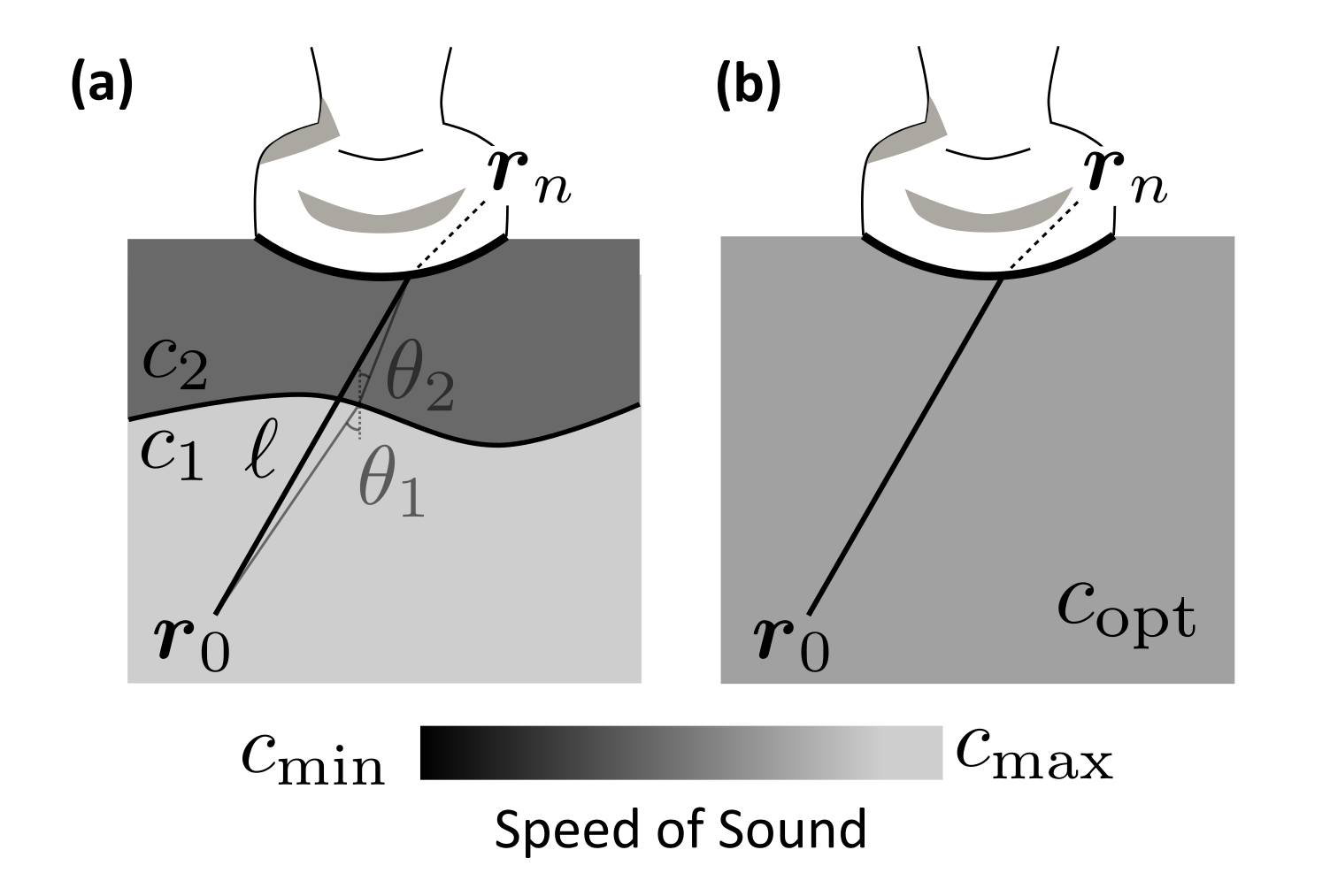
Figure 1: Geometry for finding $c_{\mathrm{opt}}$. (a) Ground truth time-of-flight delays are computed by integrating $1/c(\boldsymbol{r})$ along the straight path $\ell$. (b) The optimal SoS $c_{\mathrm{opt}}$ is the constant value which best approximates the delay ground truth profile.

Experimental Identification

The analysis above requires knowledge of the SoS distribution in the medium, such that Eq. 3 may be evaluated. However, in practice, the SoS distribution in the medium is not known, and thus the $c_{\mathrm{opt}}$ must be determined from a measure of the channel data itself, typically by a measure of the channel coherence.²⁴ The pixel intensity in the beamformed image is a convenient proxy for the coherence of the time-delayed channel signals, such that the latter, much larger data do not need to be manipulated, and has been shown to be reliable for material characterization.^{42; 37}

We define a composite metric that is the product of three component metrics, which are computed for a given region of interest (ROI) $R$, where $R\equiv\{\boldsymbol{r}~{}|~{}(x,z)\in\text{ROI}\}$ in the image beamformed at a particular sound speed. Each metric is a heuristic that measures the sharpness of the image as a function of the beamforming speed of sound $c_{0}$, and their combination is employed to ameliorate any bias any might have to a particular target type. While pure speckle may, under random phase aberration, actually become sharper due to disadvantageous side lobes in the signal correlations, this effect is slight, and is not expected in the case of vascular or structured targets.³⁶ While the three metrics measure the receive focusing quality is similar ways the combination was chosen to add robustness in case of ambiguity of a single metric for a given ROI (e.g., if its value varied only slightly over the range of $c_{\mathrm{bf}}$).

2.1.3 Image Metrics

First, we employ a version (see Appendix) of the image sharpness metric proposed by Refs. 43; 41

$$M_{S}(c_{\mathrm{bf}})=s_{1}(c_{\mathrm{bf}})\,,$$ (4)

where $s_{1}$ is the first singular value of the matrix

$$\begin{pmatrix}\big{|}&\big{|}\\ \partial I/\partial x&\partial I/\partial z\\ \big{|}&\big{|}\end{pmatrix}\,.$$ (5)

Next, the gradient metric was defined

$$M_{G}(c_{\mathrm{bf}})=\sum_{R}{\Big{\|}\nabla I(c_{\mathrm{bf}})\Big{\|}}\,,$$ (6)

where the gradient $\nabla I=(\partial I/\partial x)\boldsymbol{e}_{x}+(\partial I/\partial z)\boldsymbol{e}_{z}$ is computed with central difference approximations for the discrete derivatives. Finally, a high-pass filter is applied to the data to remove lower spatial frequency components:

$$M_{\mathrm{HP}}(c_{\mathrm{bf}})=\sum_{R}{\mathcal{F}_{k}^{-1}[\hat{I}(k\in\mathcal{K})]},$$ (7)

where $\hat{I}(k_{x},k_{z},c_{\mathrm{bf}})=\mathcal{F}_{k}[I(x,z,c_{\mathrm{bf}})]$ and $\mathcal{F}_{k}$ represents the 2D (spatial) Fourier transform. Here, $\mathcal{K}=[0.75,0.95]\,k_{\mathrm{max}}$ is the empircally selected passband of spatial frequencies, where $k_{\mathrm{max}}=\sqrt{k_{x,\mathrm{max}}^{2}+k_{z,\mathrm{max}}^{2}}$, and $k_{i,\mathrm{max}}=2\pi/\Delta x_{i}$, with $\Delta x_{i}$ as the image pixel-spacing in dimension $i$. Note that use of the 2D transform enables isolation of features that have sharp features in arbitrary directions, rather than the lateral direction only as analyzed in Ref. 40 (see Fig. A-4). The total composite metric is then defined as a product of the three component metrics

$$M=M_{\mathrm{HP}}\cdot M_{G}\cdot M_{s}\,.$$ (8)

No weighting of the component metrics is used. The optimal speed of sound was for the experimental data is then defined as the value of $c_{0}$ that maximizes the total metric $M$

$$c_{\mathrm{opt}}=\arg\,\max_{c_{0}}M(c_{0})\,;$$ (9)

see Fig. 2. To preserve computational efficiency, images were beamformed by setting the receive beamforming SoS with step size $\Delta c_{0}=$10\text{\,}\mathrm{m}\mathrm{/}\mathrm{s}$$. The image stack was then interpolated to $1\text{\,}\mathrm{m}\mathrm{/}\mathrm{s}$, as the pixel intensity varied smoothly. To preserve scaling between the images, the depth mapping was scaled according to $\Delta z\rightarrow\Delta z(c_{\mathrm{bf}}/c_{\mathrm{ref}})$.

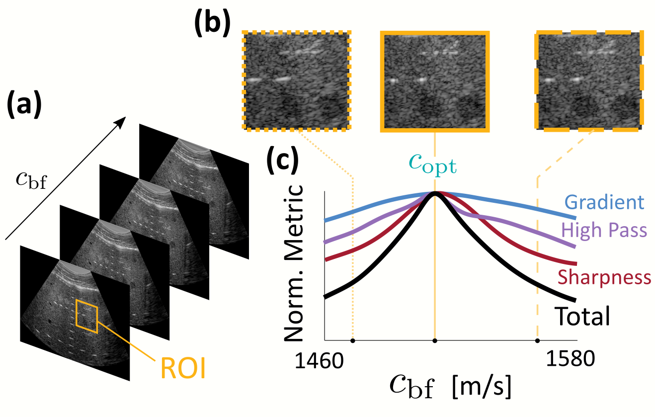
Figure 2: Identification of experimental $c_{\mathrm{opt}}$ from image metrics. (a) Time series RF data are beamformed via conventional DAS at a range of beamforming sound speeds $c_{\mathrm{bf}}$. A relevant ROI is selected. (b) The image (pixel) data within the ROI at each $c_{\mathrm{bf}}$ are used to compute three component image metrics. (c) The product of the three image metrics is defined as the total metric [Eq. 8], whose maximum value is taken as the position of $c_{\mathrm{opt}}$.

2.2 In Vitro, Ex Vivo, and In Vivo Experiments

For the experimental data, harmonic channel data were acquired with a commercial ultrasound system (GE LOGIQ E10, GE Healthcare, Chicago, IL, USA) and a tissue-mimicking ultrasound phantom (Model 040GSE, CIRS, Norfolk, VA USA), using a curvilinear abdominal probe (GE C1-6-D, $3.5\text{\,}\mathrm{M}\mathrm{H}\mathrm{z}$ center frequency, 192 elements, $350\text{\,}\mathrm{\SIUnitSymbolMicro m}$ pitch, $66\text{\,}\mathrm{m}\mathrm{m}$ elevation focus) with default abdominal settings ($3.0\text{\,}\mathrm{M}\mathrm{H}\mathrm{z}$). A dynamic aperture was applied to the resulting IQ data, which were delayed at a constant speed of sound for each scan line acquisition ($N=210$). The final image stack $I(\boldsymbol{r},c_{\mathrm{bf}})$ represents the scan-converted images for each bulk SoS . Aberration was induced using material layers positioned between the surface of the phantom and the probe. The layers included: a gel layer $3\text{\,}\mathrm{c}\mathrm{m}$ thick, with scatters (custom, $0.5\text{\,}\mathrm{\char 37\relax}$ volume fraction $50\text{\,}\mathrm{\SIUnitSymbolMicro m}$ glass beads, gel speed of sound approximately $1450\text{\,}\mathrm{m}\mathrm{/}\mathrm{s}$, Sun Nuclear, Melbourne, FL, USA); as well as ex vivo porcine fat samples obtained from supermarket butchers, selected visually for fat and fascia distribution. The animal fat layers were heated in water bath to approximately $37\text{\,}\mathrm{\SIUnitSymbolDegree}\mathrm{C}$ to best approximate realistic in vivo material properties. Finally, in vivo images of the gallbladder were collected from healthy volunteers following verbal consent ($N=4$, MGH IRB approval 2022P000850) with (for those with small skin-to-capsule distances) and without (for those with more inherent aberration) the gel aberrator.

3 Results

3.1 Effect of Geometry on Optimal SoS

The optimal SoS was determined from Eq. 3 for a typical imaging field that $8\text{\,}\mathrm{c}\mathrm{m}$ laterally by $12.5\text{\,}\mathrm{c}\mathrm{m}$ axially in a medium with SoS of $1540\text{\,}\mathrm{m}\mathrm{/}\mathrm{s}$, immediately beneath a layer with SoS $c_{\ell}$, thickness $d$, and with an aperture governed by $F\#$; see Fig. 3.

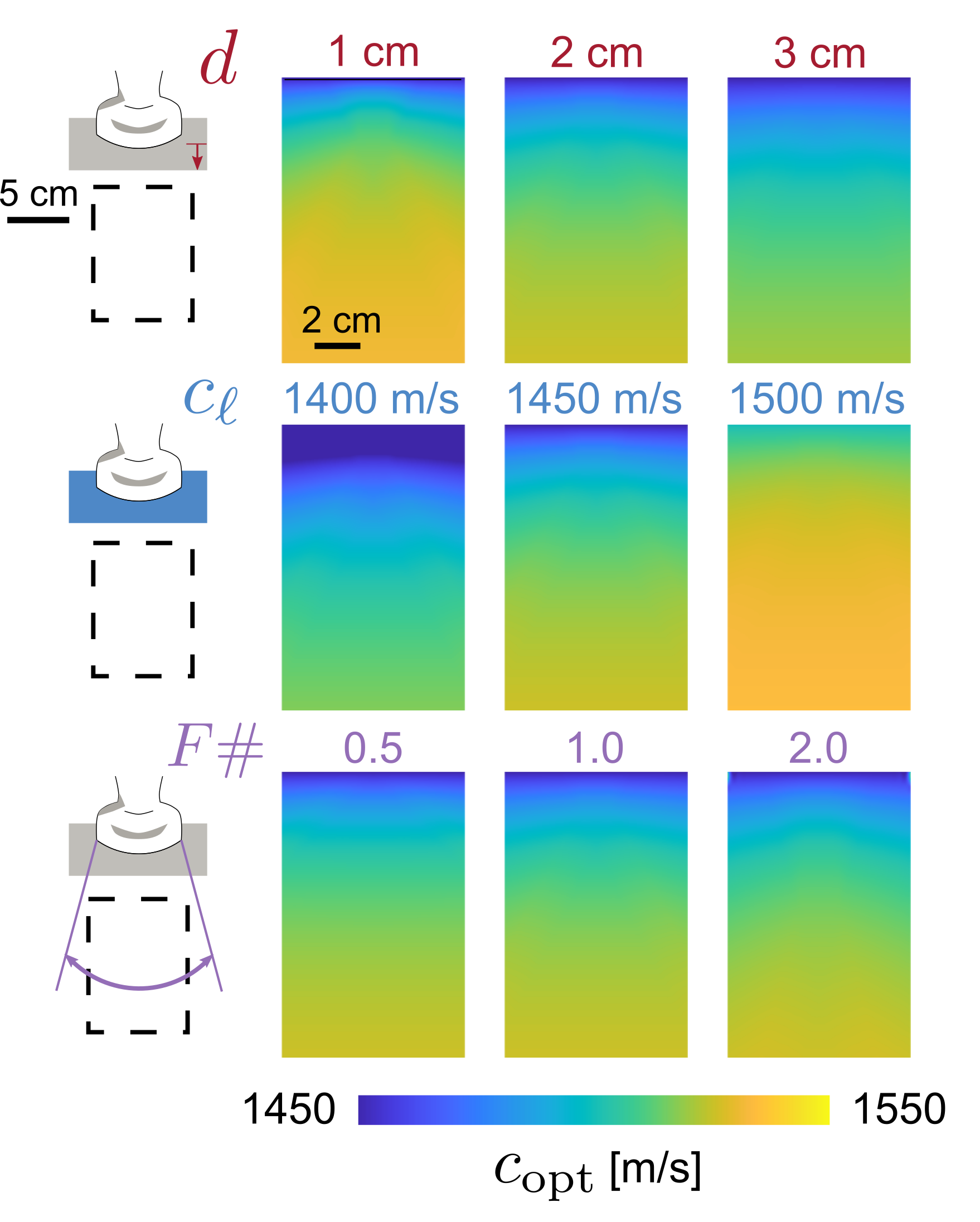
Figure 3: Spatial variation in the optimal beamforming SoS $c_{\mathrm{opt}}$ [calculated from Eq. 3]. Values calculated for the region indicated at left, and for the indicated layer thicknesses, layer SoS $c_{\ell}$, and receiving aperture for the indicated $F\#$. The center column represents the default values for each parameter.

For a constant layer SoS $c_{\ell}=$1450\text{\,}\mathrm{m}\mathrm{/}\mathrm{s}$$ (top row), thinner layers introduced larger spatial gradient in $c_{\mathrm{opt}}$ (i.e., the value of $c_{\mathrm{opt}}$ varied more rapidly in space). However in these cases the value of $c_{\mathrm{opt}}$ was on average closer to $1540\text{\,}\mathrm{m}\mathrm{/}\mathrm{s}$. For a constant layer thickness of $d=$2\text{\,}\mathrm{c}\mathrm{m}$$ (middle row), the spatial distribution of $c_{\mathrm{opt}}$ was similar for various $c_{\ell}$, however slower layer SoS lowered $c_{\mathrm{opt}}$, especially immediately below the layer. When both $c_{\ell}$ and $d$ were fixed, the aperture size (defined from the $F\#$ did not have a large influence on the distribution or value of $c_{\mathrm{opt}}$ (bottom row).

While the value of $c_{\mathrm{opt}}$ varied relatively smoothly with position, the goodness of this value must also be established. That is, the value that optimizes Eq. 3 may still produce unacceptably large errors in the beamforming delays, compared to the true time of flight. Therefore, we also considered the arrival time error for delays calculated with $c_{\mathrm{opt}}$ over the same region, with various layer thicknesses $d$ and SoSs $c_{\ell}$; results are shown in Fig. 4.

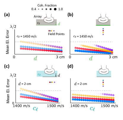
Figure 4: Mean per-element arrival time error magnitude compared to ground truth (i.e., $\left\|\tau_{n}-\tau^{g}_{n}\right\|$, where geometric delays are computed with $c_{\mathrm{opt}}$) at the indicated positions. The size and transparency indicates the coherent aperture fraction at the given $c_{\mathrm{opt}}$. Reported in wavelengths $\lambda$ for $3\text{\,}\mathrm{M}\mathrm{H}\mathrm{z}$ ($333\text{\,}\mathrm{n}\mathrm{s}$), and for $F\#=1.41$. (a) Mean per-element error for a layer with $c_{\ell}=$1450\text{\,}\mathrm{m}\mathrm{/}\mathrm{s}$$ at the indicated axial and (b) transverse positions as a function of the layer thickness $d$. (c) Mean per-element error for a layer with $d=$2\text{\,}\mathrm{c}\mathrm{m}$$ at the indicated axial and (d) transverse positions as a function of the layer SoS $c_{\ell}$.

Interestingly, the mean arrival time error was largest for thinner layers, and decreases with $d$ [Fig. 4(a–b)]. This is likely because thinner layers introduce more rapid spatial variation in the aberration profile across the face of the transducer, which cannot be fully accounted for by any $c_{\mathrm{opt}}$. However, we note that the fraction of the aperture (see definition below) that could be made coherent with a single $c_{\mathrm{opt}}$ increased with $d$, as the point-to-point variation in optimal SoS varies less with thicker layers (Fig. 3). The influence of layer SoS for a fixed layer thickness $d=$2\text{\,}\mathrm{c}\mathrm{m}$$, also decreased monotonically with $c_{\ell}$, expectantly vanishing as $c_{\ell}$ approaches the SoS in the underlying medium [Fig. 4(c–d)]. In all cases, we find an optimal SoS may achieve acceptably small mean errors (less than $\lambda/4$ at $3\text{\,}\mathrm{M}\mathrm{H}\mathrm{z}$ or $83\text{\,}\mathrm{n}\mathrm{s}$) for uniform layers with realistic thicknesses and speeds of sound, and performance is generally improved on-axis and for faster, thicker layers.

Finally, the mean receive delay error per element at the determined $c_{\mathrm{opt}}$ may be less than $\lambda/4\,(=$67\text{\,}\mathrm{n}\mathrm{s}$$ at $$3\text{\,}\mathrm{M}\mathrm{H}\mathrm{z}$)$ for relevant layer depths and thicknesses. Therefore we considered the size of the coherent aperture for these geometries. We defined the coherent aperture fraction as the ratio of the largest number of contiguous elements with round trip arrival time errors less than 0.2$\lambda$ (i.e., slightly less than the destructive interference that would occur for $\lambda/4$), relative to the number of receive elements used for a given position and $F\#$. For instance, 96 of the 192 elements may be active in receiving for a given $F\#$; if the longest subset of adjacent elements with error less than $\lambda/5$ is 48, then the corresponding coherent aperture fraction would be 48/96 = $50\text{\,}\mathrm{\char 37\relax}$.

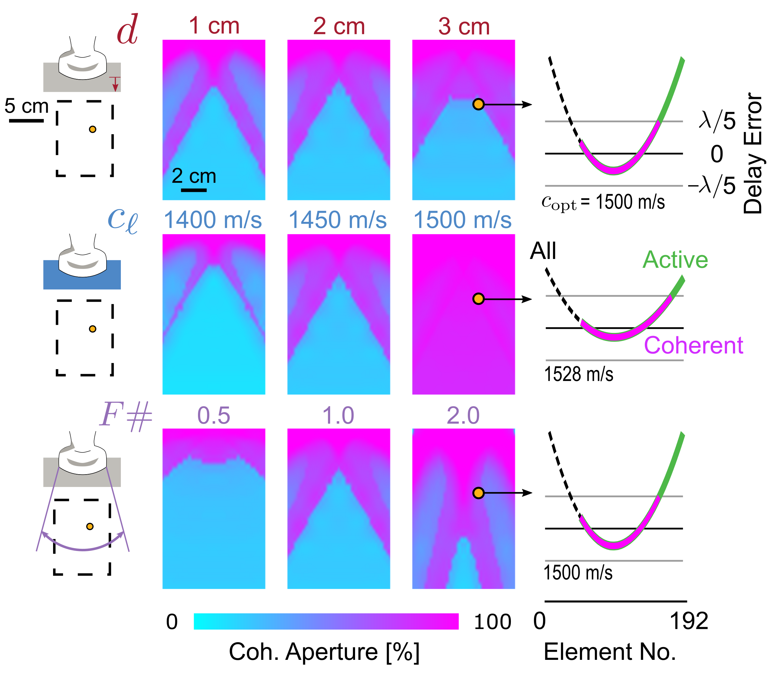
Figure 5: Spatial variation in the coherent aperture for $c_{\mathrm{bf}}=c_{\mathrm{opt}}$ in the region indicated at left, for the indicated layer thicknesses, layer SoS $c_{\ell}$, and receiving aperture for the indicated $F\#$. The center column represents the default values for each parameter. At right is the arrival time error for each element at the identified $c_{\mathrm{opt}}$ for the location marked by the orange dot. The active aperture is shown in green, compared with the coherent fraction (from the colorscale). The wavelength (period) is computed for $3\text{\,}\mathrm{M}\mathrm{H}\mathrm{z}$.

In general, the layer SoS $c_{\ell}$ had the most pronounced effect on the coherent aperture fraction: Slower layers impart more rapidly changing delay profiles across the face of the array (and thus $c_{\mathrm{opt}}$ varies rapidly with position), and thus $c_{\mathrm{opt}}$ is valid over smaller portions of the active aperture. However, as seen in Fig. 4 points nearer the array are more likely to have a $c_{\mathrm{opt}}$ that achieves a large coherent aperture fraction. If larger $F\#$ are used, the total delay error needs to be optimized over smaller number of elements, and therefore the fraction of these elements that are coherent at $c_{\mathrm{opt}}$ is increased.

3.2 Image Metrics

Because our analysis showed that that an optimal SoS with a mean receive arrival time error of less than a quarter period (at $3\text{\,}\mathrm{M}\mathrm{H}\mathrm{z}$) was feasible for layered geometry and relevant dimensions and apertures, we sought to verify that such a $c_{\mathrm{opt}}$ could be identified from the proposed metrics, and that the resulting images offered improvement compared to the uncorrected images.

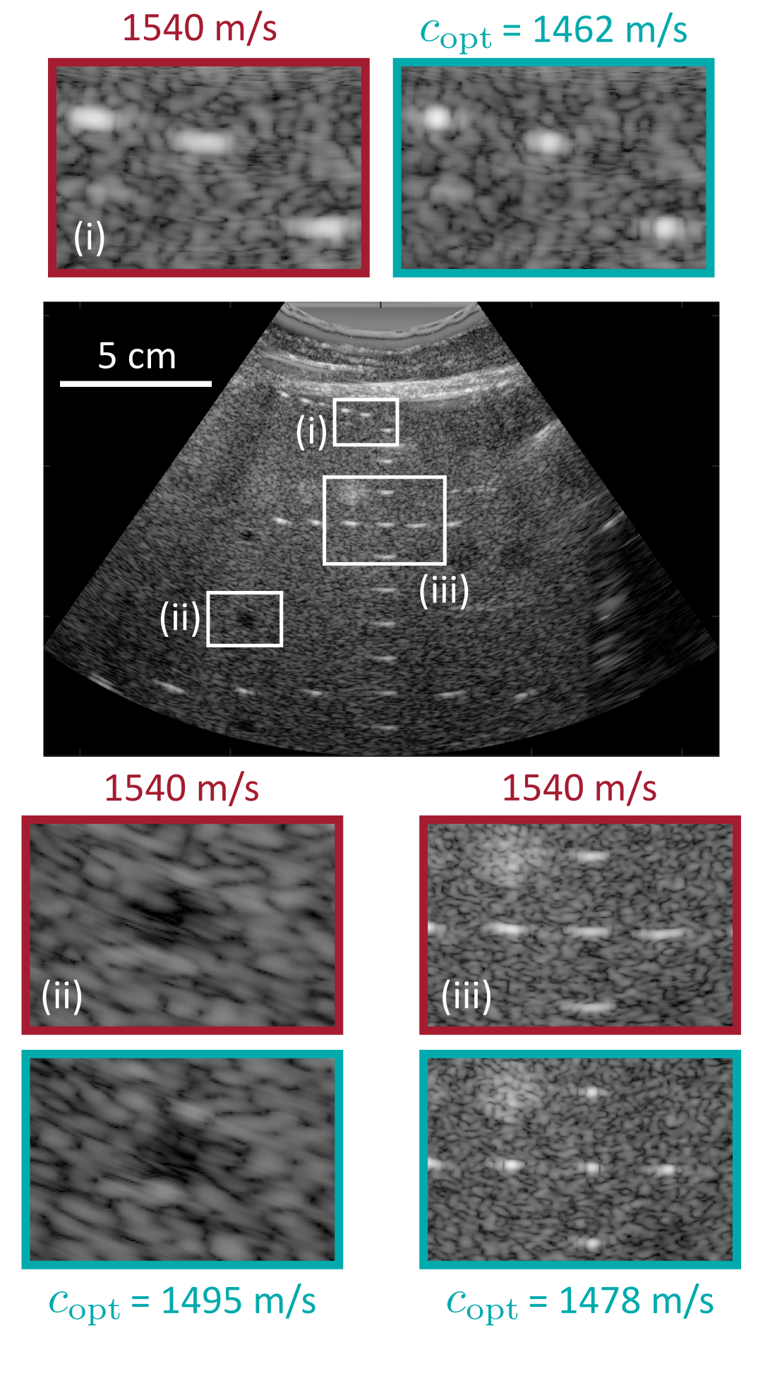
Figure 6: Example image for a phantom imaged with a $3.5\text{\,}\mathrm{c}\mathrm{m}$ fat layer. For each ROI (white boxes) the total metric was computed to identify $c_{\mathrm{opt}}$, and the image beamformed with this SoS is shown.

Qualitatively, image regions beamformed at the metric-identified $c_{\mathrm{opt}}$ were superior to the aberrated image at the default $1540\text{\,}\mathrm{m}\mathrm{/}\mathrm{s}$. Specifically, pin targets were most noticeably improved, while contrast targets varied less with changing $c_{\mathrm{bf}}$ (with some improved demarcation of anechoic region boundaries, as shown in Fig. 6). Additionally, provided the ROI included the target structure in all images formed over the range of $c_{\mathrm{bf}}$, the identified $c_{\mathrm{opt}}$ and metric trends were observed to be robust to target type and ROI size (Fig. A-3).

To quantify this improvement, for each dataset, 11 targets (six point targets and five contrast targets, $1\text{\,}\mathrm{c}\mathrm{m}$ to $10\text{\,}\mathrm{c}\mathrm{m}$ below the fat layer) were demarcated, and the $c_{\mathrm{opt}}$ values were determined from Eq. 9.

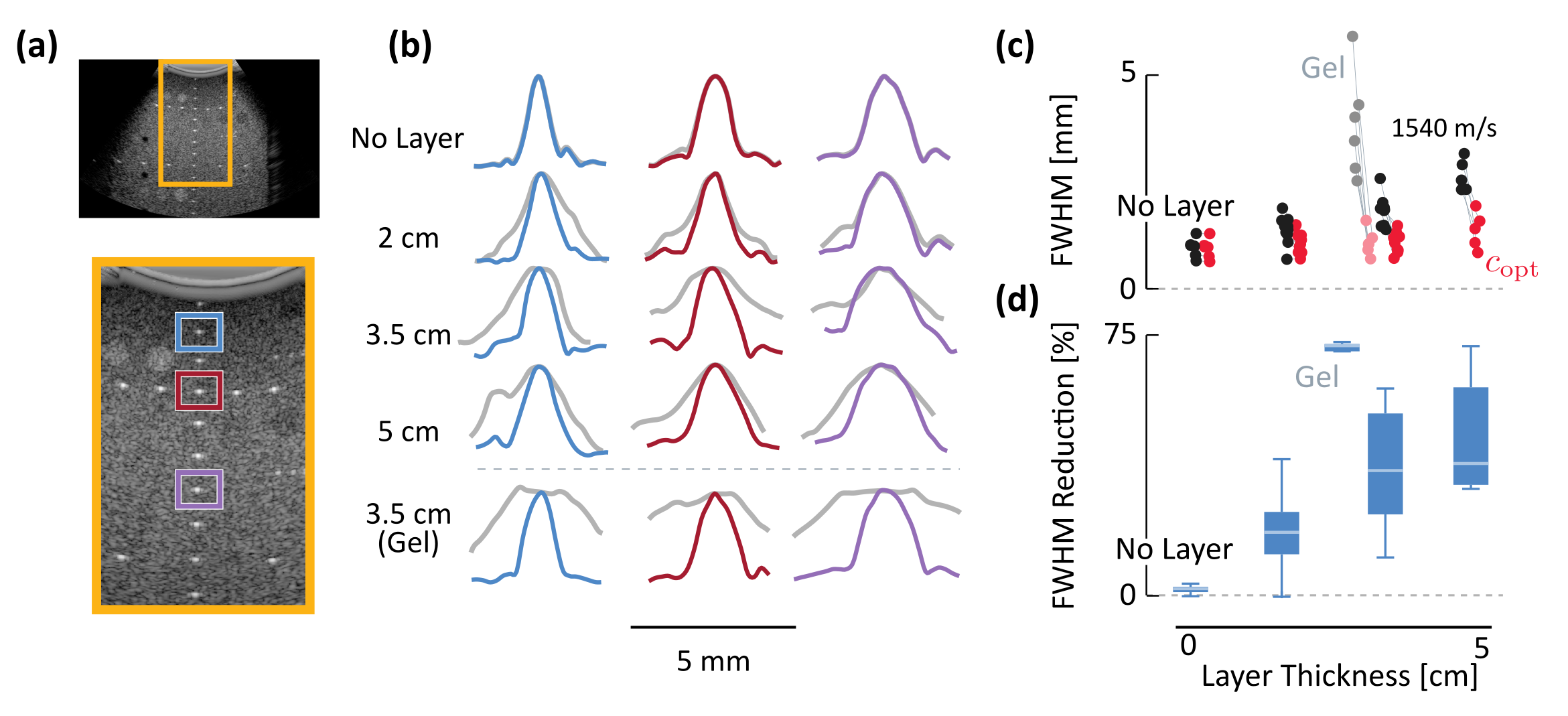
Figure 7: Identification of experimental $c_{\mathrm{opt}}$ with image metrics. (a) Unaberrated image of the US phantom with inset showing position of pin targets evaluated in (b) for their FWHM. (b) Profiles of the indicated pins from (a). Color: in the image formed with the metric-identified $c_{\mathrm{opt}}$. Gray: in the image formed with $1540\text{\,}\mathrm{m}\mathrm{/}\mathrm{s}$. Each row corresponds to data from the indicated thickness fat layer. (c) Change in FWHM of pins (6 per image) between the $1540\text{\,}\mathrm{m}\mathrm{/}\mathrm{s}$ image and the $c_{\mathrm{opt}}$ image. (d) Relative reduction in the FWHM of the points in (c).

Over the range of pin resolution targets in the phantom, the identified $c_{\mathrm{opt}}$ reduced the lateral FWHM in the resulting image by $38\pm 22\text{\,}\mathrm{\char 37\relax}$ compared to the image formed with $1540\text{\,}\mathrm{m}\mathrm{/}\mathrm{s}$. The improvement was especially pronounced for the more uniform gel layer case [Fig. 7(c–d)]. Generally, the benefit of the correction increased with depth (i.e., deeper targets had greater FWHM reduction relative to the default case), as well as with thicker layers. These is consistent with the results are consistent with the previous analysis, which indicated for a uniform layer, $c_{\mathrm{opt}}$ was most valid for larger values of $d$ and depths Fig. 4. The contrast-to-noise ratio of the resulting images, however, was essentially unchanged between the $c_{\mathrm{opt}}$ and $1540\text{\,}\mathrm{m}\mathrm{/}\mathrm{s}$ images (difference $0.0\pm 0.05\text{\,}\mathrm{d}\mathrm{B}$). This is likely due to the much slower variation in contrast with the beamforming SoS and F-number compared to point target FWHM ³⁹.

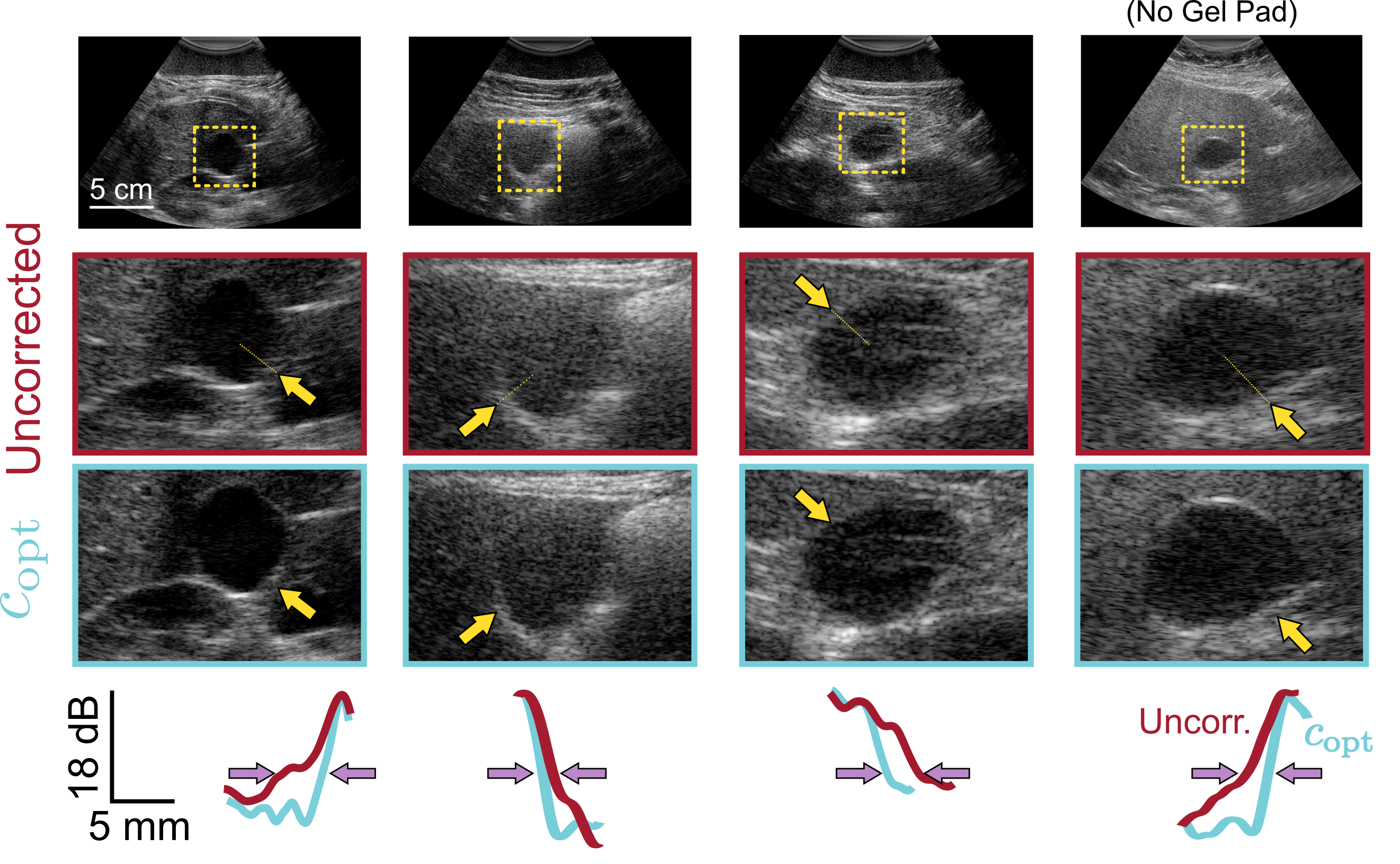
Figure 8: Aberrated and corrected images of in vivo gallbladders at $3\text{\,}\mathrm{M}\mathrm{H}\mathrm{z}$. Columns 1–3: healthy livers with the gel aberrator; Column 4: suspected NAFLD without added aberration. Top row: Default images ($1540\text{\,}\mathrm{m}\mathrm{/}\mathrm{s}$) with metric ROIs indicated in yellow. Second row: ROI of uncorrected image. Third row: ROI of image formed with metric identified $c_{\mathrm{opt}}$. Note increased sharpness of gallbladder walls (yellow arrows) and reduced clutter within. Bottom row: mean intensities from 10 parallel profiles (spacing $0.1\text{\,}\mathrm{c}\mathrm{m}$) at the positions of the yellow arrows. All image dynamic ranges are $54\text{\,}\mathrm{d}\mathrm{B}$.

Figure 8 shows representative in vivo gallbladder imaging results from 4 volunteers. In all cases, the aberrator was seen to blur liver structures, particularly near vessel and gallbladder boundaries (row 2). Following identification of the optimal SoS via Eq. 9, edges were noticeably sharper: the intensity gradient at the indicated gallbladder walls was larger by a factor of 0.75$\pm$0.88 (bottom row, Fig. 8). Consistent with in vitro results, the contrast was improved only slightly (per instance improvement of $1.5\pm 1.5\text{\,}\mathrm{\char 37\relax}$), though this result may be improved, e.g., by weighting with the new channel coherence, which is expected to be more reliable at $c_{\mathrm{bf}}$.

Finally, we assessed the computational efficiency of the method. Data beamformed at $10\text{\,}\mathrm{m}\mathrm{/}\mathrm{s}$ were seen to allow sufficiently accurate interpolation of the images [mean normalized pixel intensity difference $(0.16\pm 9.3)\times 10^{-3}$ between interpolated and beamformed images]. Thus given DAS beamformer outputs for approximately 10 equally spaced $c_{\mathrm{bf}}$ (e.g., 1460 to $1550\text{\,}\mathrm{m}\mathrm{/}\mathrm{s}$), $c_{\mathrm{opt}}$ may be determined to within $1\text{\,}\mathrm{m}\mathrm{/}\mathrm{s}$ from the image metrics; for the work described herein, this required $91.8\pm 20.6\text{\,}\mathrm{\SIUnitSymbolMicro s}$ per pixel with minimally optimized matlab code (32 GB RAM, Intel 10 cores at 2.8 GHz). Overall efficiency could also be improved by performing the beamforming with only the ROI to identify $c_{opt}$.

4 Discussion

In this work, we established the feasibility and applicability bounds of a single optimal receive beamforming SoS to achieve appreciably low delay errors, and to enhance image quality at scales and geometries relevant to abdominal ultrasound. Through analytical methods, we found that the optimal SoS varies largely with the axial direction, and that we could achieve per-element error of less than a quarter period for a curved array at $3.0\text{\,}\mathrm{M}\mathrm{H}\mathrm{z}$. Thicker layers, those with SoS similar to the underlying medium, and narrower apertures (larger $F\#$) resulted the smallest arrival time errors for the optimal SoS compared to the ray calculations, consistent with previous work ³⁴; see Figs. 3, 4 and 5. For in vitro data, we found the experimentally identified $c_{\mathrm{opt}}$ reduced the point spread function by up to $75\text{\,}\mathrm{\char 37\relax}$ (Figs. 6 and 7) compared to the uncorrected case, and increased sharpness of organ walls was observed in vivo (Fig. 8). Thus identification of an optimal receive SoS with the image-based metric represents a simple and effective means to improve abdominal ultrasound images.

The proposed method does have several limitations. First, the analysis assumes a uniform layer and thus ignores any morphological complexity of the layers, which can have important effects on the uniformity and distribution of the arrival time errors.^{44; 45} Additionally, random phase errors, or more complicated geometries (e.g., a layer of varying thickness) result in delay profiles which cannot be well approximated by a single SoS curve. Furthermore, the scheme considers only manipulation of the receive delays; this which enables its use with focused imaging (as here) or unfocused (e.g., plane wave imaging⁴⁶) techniques. Further improvement (and agreement with the analysis) might be seen if adjustment of the transmit pattern were also incorporated.

We note finally that as a means determine an optimal bulk SoS, this technique also may be used as a starting point for other techniques. For instance, minimum variance beamforming^{47; 48} or coherence-based techniques^{28; 29; 49} may provide greater benefit with initial data delayed at $c_{\mathrm{opt}}$. Methods for identification of phase shifts from channel correlations^{50; 18; 16} or matrix imaging techniques^{20; 51} also would be aided, since the expected magnitude of the delay corrections would be smaller relative to those found from $1540\text{\,}\mathrm{m}\mathrm{/}\mathrm{s}$.

5 Conclusions

In this work we have demonstrated that a single, optimal receive beamforming SoS may provide significant improvement in aberrated US images. Specifically, for layered geometries at frequencies relevant to abdominal US, mean arrival time errors less than a fifth of a wavelength were attainable. In experiments with layered abberators, image metrics (which use only conventional DAS beamformer outputs) reliably identified an optimal SoS for ROIs, and improved point target resolution by $60\text{\,}\mathrm{\char 37\relax}$. Together, these results indicate that identification of $c_{\mathrm{opt}}$ may have immediate application to clinical application and allow improved abdominal imaging among populations for whom it is most crucial.

Appendix

Appendix A Sharpness Metric

Reference 43 proposes the metric

$$M_{S}=\frac{\sqrt{s_{1}^{2}+\xi N^{2}\sigma^{2}}}{\epsilon+\sigma^{2}}\,,$$ (A-1)

where $N^{2}$ is the number of pixels in the ROI, $\sigma^{2}$ is the variance of the zero mean Gaussian white noise, $\xi\sim 1/2$ is a scaling factor that depends on the nature of the calculation of the numerical gradients, and $\epsilon$ is a small positive constant to prevent a vanishing denominator. Recall here that $s_{1}$ is the first singular value of the matrix

$$\begin{pmatrix}\big{|}&\big{|}\\ \partial I/\partial x&\partial I/\partial z\\ \big{|}&\big{|}\end{pmatrix}\,,$$ (A-2)

where $I$ is the pixel intensity. We may approximate

$$M_{S} =s_{1}\frac{\left[1+\xi(N\sigma)^{2}/s_{1}^{2}\right]^{\frac{1}{2}}}{\epsilon+\sigma^{2}}$$

$$\simeq s_{1}\left[\frac{1+(N\sigma)^{2}/2s_{1}^{2}}{\epsilon+\sigma^{2}}\right]\,.$$ (A-3)

where the factor of $\xi$ has been dropped since we are interested in the order of the second term in the numerator. If we assume that we have small variance in the signal compared to the magnitude of the first singular value, then, this reduces to $M_{s}=s_{1}/(\epsilon+\sigma^{2})\approx s_{1}/\epsilon$. Therefore, it is safe to use the first singular value as the metric, provided the noise and ROI are sufficiently small. Reference 41 showed the validity of this technique to estimate the speed of sound for homogeneous media.

Appendix B Transverse and Elevational Delays

Call the positions of the individual transducer elements $\boldsymbol{r}_{i}^{\prime}$, and the positional coordinate is $\boldsymbol{r}$. The vector that points from $\boldsymbol{r}$ to $\boldsymbol{r}^{\prime}$ will be defined $\leavevmode\resizebox{}{5.59721pt}{ \leavevmode\hbox to7.43pt{\vbox to6.03pt{\text{[drawing]}}}}=\boldsymbol{r}-\boldsymbol{r}^{\prime}$. The coordinate system is not very important, except that the interface between the layer and the capsule is parallel to the $x$-$y$ plane. For convenience we’ll say the reference transducer element (e.g., the center element) is at the origin. See Fig. A-1

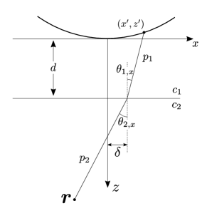
Figure A-1: Geometry for solving for the ray.

Now, consider a ray originating at $\boldsymbol{r}$ and arriving at $\boldsymbol{r}^{\prime}$, as viewed looking along the $y$-axis (i.e., the visible space is parallel to the $x$-$z$ plane); see Fig. A-1. The ray will be refracted at the interface according to Snell’s law

$$\frac{\sin{\theta_{1,x}}}{c_{1}} =\frac{\sin{\theta_{2,x}}}{c_{2}}\,,$$ (A-4)

where $c_{1}$ is the speed of sound in the layer, and $c_{2}$ in the liver. Now because the $x$-distance between the two points $\boldsymbol{r}$ and $\boldsymbol{r}^{\prime}$ is known, we have

$$x-x^{\prime} =d\tan{\theta_{1,x}}+(z-d)\tan{\theta_{2,x}}\,.$$ (A-5)

Now, Eq. A-4 and Eq. A-5 form a system of equations of two equations for two unknowns, which may be solved for $\theta_{x,1}$ and $\theta_{x,2}$.

By the same reasoning, we have for the $y$-direction

$$y-y^{\prime} =d\tan{\theta_{1,y}}+(z-d)\tan{\theta_{2,y}}\,.$$ (A-6)

subject to

$$\frac{\sin{\theta_{1,y}}}{c_{1}} =\frac{\sin{\theta_{2,y}}}{c_{2}}\,,$$ (A-7)

Once we have determined $\theta_{x,1}$, $\theta_{x,2}$, $\theta_{y,1}$, $\theta_{y,2}$ from Eqs. A-4, A-5, A-7 and A-6, we can compute the travel time $\tau_{l}$ of the ray along the path from $\boldsymbol{r}$ to $\boldsymbol{r}^{\prime}$. The travel time in the layer is

$$\tau_{1} =\sqrt{d^{2}+\left[d\tan{\theta_{x,1}}\right]^{2}+\left[d\tan{\theta_{y,1}}\right]^{2}}\bigg{/}c_{1}$$

$$=d\sqrt{1+\tan^{2}{\theta_{x,1}}+\tan^{2}{\theta_{y,1}}}\bigg{/}c_{1}\,.$$ (A-8)

The travel time in the liver

$$\tau_{2} =\sqrt{(z-d)^{2}+\left[(z-d)\tan{\theta_{x,2}}\right]^{2}+\left[(z-d)\tan{\theta_{y,2}}\right]^{2}}\bigg{/}c_{2}$$

$$=(z-d)\sqrt{1+\tan^{2}{\theta_{x,2}}+\tan^{2}{\theta_{y,2}}}\bigg{/}c_{2}\,.$$ (A-9)

Now in the no layer case, the travel time is simply

$$\tau_{0} =\|\boldsymbol{r}-\boldsymbol{r}^{\prime}\|\Big{/}c_{2}$$

$$=\leavevmode\resizebox{}{5.38193pt}{ \leavevmode\hbox to7.24pt{\vbox to5.64pt{\text{[drawing]}}}}/c_{2}\,.$$ (A-10)

Thus, the additional time delay is

$$\tau_{l}=\tau_{1}+\tau_{2}-\tau_{0}.$$ (A-11)

In the case of a curved array, the $d$ in Eqs. A-5, A-6 and A-8 is replaced by $d\rightarrow d-z^{\prime}$.

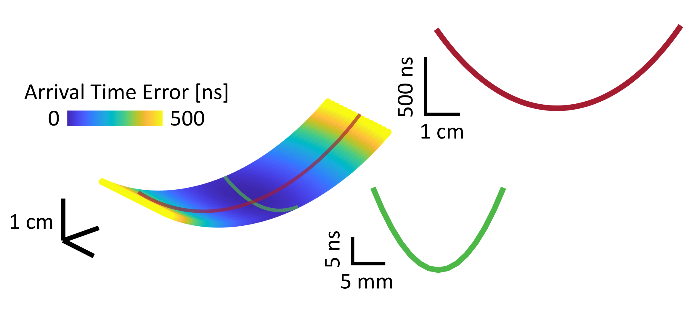
Figure A-2: Variation in arrival time error in the transverse (red) and elevational (green) directions; note the hundredfold difference in vertical scale. Calculations are from Eq. A-11 for a $2\text{\,}\mathrm{c}\mathrm{m}$ layer with speed of sound $c_{1}=$1450\text{\,}\mathrm{m}\mathrm{/}\mathrm{s}$$.

A result for a $2\text{\,}\mathrm{c}\mathrm{m}$ layer with a curvilinear array is shown in Fig. A-2. Note the more than tenfold difference in the gradient between the two, suggesting the transverse (i.e., element-direction) variation has the largest effect.

Appendix C Effect of ROI and Bandwidth on Metrics

In general, the heuristic component and composite metrics given by Eqs. (4–8) were robust to target type and ROI size. While the trend of a metric may be obscured by portions structures that move into or out of the ROI as $c_{\mathrm{bf}}$ varies (e.g., a pin target’s spread as $c_{\mathrm{bf}}$ is far from $c_{\mathrm{opt}}$), they were generally restored with an ROI that comprised the structures of interest.

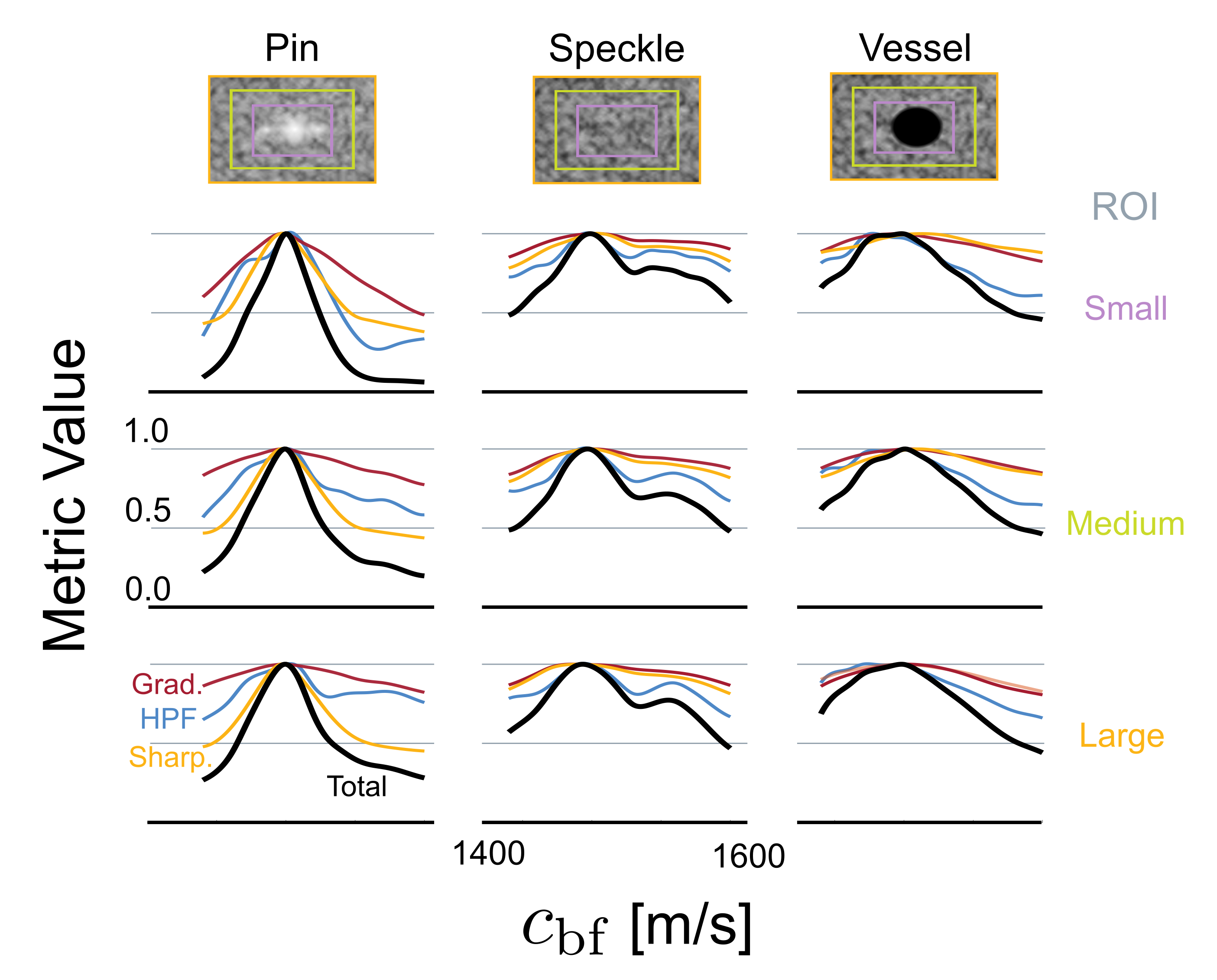
Figure A-3: Example metrics $M(c_{\mathrm{bf}})$ for various target types and ROI sizes. Data are for the CIRS phantom with 5 cm fat layer at 3 MHz.

Additionally, the high pass filter metric is similar to that used in Ref. 40, and requires a choice of spatial bandwidth. However, that work considered only the 1D lateral transform (i.e., function of $k_{x}$ only) at each depth, and thus energy in particular bands is associated with intensity variation only in the transverse direction. The high pass filter metric considers energy in a 2D spatial bandwidth, which may correspond to sharp transitions in any orientation. This is especially important, e.g., for vessel walls.

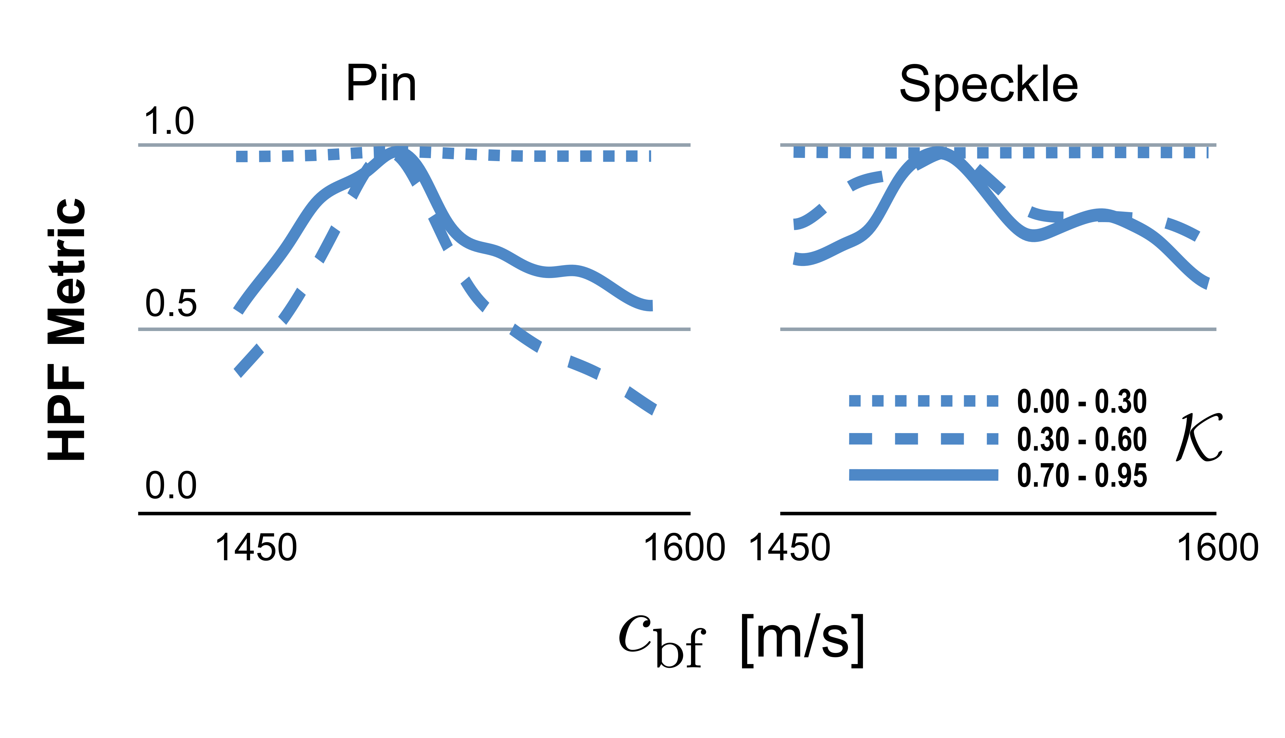
Figure A-4: Effect of bandwidth on the value of the high-pass filter metric $M_{HP}(c_{\mathrm{bf}}$ for the indicated target type and ROI sizes. Data are for the CIRS phantom with 5 cm fat layer at 3 MHz.

Figure A-4 shows the effect of the chosen bandwidth $\mathcal{K}$ on the resulting metric. Using lower spatial frequencies results in a metric that varies little with $c_{[}\mathrm{bf}]$, as large-scale features of the image are relatively constant. However, for higher bandwidths, features to be resolved posses more variable spectral content as they move in and out of focus, resulting in clearer trends in the metric and more reliable identification of $c_{\mathrm{opt}}$.

References

- 1 John S. Rose. Ultrasound in abdominal trauma. Emergency Medicine Clinics, 22(3):581–599, August 2004.
- 2 Bahaa M. Fadel, Dania Mohty, Brigitte E. Kazzi, Bandar Alamro, Fatima Arshi, Manal Mustafa, Najmeddine Echahidi, and Victor Aboyans. Ultrasound Imaging of the Abdominal Aorta: A Comprehensive Review. Journal of the American Society of Echocardiography, 34(11):1119–1136, November 2021.
- 3 Vanja Giljaca, Tin Nadarevic, Goran Poropat, Vesna Stefanac Nadarevic, and Davor Stimac. Diagnostic Accuracy of Abdominal Ultrasound for Diagnosis of Acute Appendicitis: Systematic Review and Meta-analysis. World Journal of Surgery, 41(3):693–700, March 2017.
- 4 Vijay Pandyarajan, Robert G. Gish, Naim Alkhouri, and Mazen Noureddin. Screening for Nonalcoholic Fatty Liver Disease in the Primary Care Clinic. Gastroenterology & Hepatology, 15(7):357–365, July 2019.
- 5 Naga Chalasani, Zobair Younossi, Joel E. Lavine, Michael Charlton, Kenneth Cusi, Mary Rinella, Stephen A. Harrison, Elizabeth M. Brunt, and Arun J. Sanyal. The diagnosis and management of nonalcoholic fatty liver disease: Practice guidance from the American Association for the Study of Liver Diseases. Hepatology, 67(1):328–357, 2018.
- 6 Chris Estes, Homie Razavi, Rohit Loomba, Zobair Younossi, and Arun J. Sanyal. Modeling the epidemic of nonalcoholic fatty liver disease demonstrates an exponential increase in burden of disease. Hepatology, 67(1):123–133, 2018.
- 7 Alina M. Allen, Holly K. Van Houten, Lindsey R. Sangaralingham, Jayant A. Talwalkar, and Rozalina G. McCoy. Healthcare Cost and Utilization in Nonalcoholic Fatty Liver Disease: Real-World Data From a Large U.S. Claims Database. Hepatology, 68(6):2230–2238, 2018.
- 8 Ruben Hernaez, Mariana Lazo, Susanne Bonekamp, Ihab Kamel, Frederick L. Brancati, Eliseo Guallar, and Jeanne M. Clark. Diagnostic accuracy and reliability of ultrasonography for the detection of fatty liver: A meta-analysis. Hepatology, 54(3):1082–1090, 2011.
- 9 Valeria Cuzmar, Gigliola Alberti, Ricardo Uauy, Ana Pereira, Cristián García, Florencia De Barbieri, Camila Corvalán, JosĂŠ L. Santos, VerĂłnica Mericq, Luis Villarroel, and Juan CristĂłbal Gana. Early Obesity: Risk Factor for Fatty Liver Disease. Journal of Pediatric Gastroenterology and Nutrition, 70(1):93–98, January 2020.
- 10 Stergios A. Polyzos, Jannis Kountouras, and Christos S. Mantzoros. Obesity and nonalcoholic fatty liver disease: From pathophysiology to therapeutics. Metabolism, 92:82–97, March 2019.
- 11 Raiya Sarwar, Nicholas Pierce, and Sean Koppe. Obesity and nonalcoholic fatty liver disease: current perspectives. Diabetes, Metabolic Syndrome and Obesity: Targets and Therapy, 11:533–542, September 2018.
- 12 Alessandro de Moura Almeida, Helma Pinchemel Cotrim, Daniel Batista Valente Barbosa, Luciana Gordilho Matteoni de Athayde, Adimeia Souza Santos, Almir GalvĂŁo Vieira Bitencourt, Luiz Antonio Rodrigues de Freitas, Adriano Rios, and Erivaldo Alves. Fatty liver disease in severe obese patients: Diagnostic value of abdominal ultrasound. World Journal of Gastroenterology : WJG, 14(9):1415–1418, March 2008.
- 13 ClĂĄudio C. Mottin, Myriam Moretto, Alexandre V. Padoin, Aline M. Swarowsky, Marcelo G. Toneto, Luiz Glock, and Giuseppe Repetto. The role of ultrasound in the diagnosis of hepatic steatosis in morbidly obese patients. Obesity Surgery, 14(5):635–637, May 2004.
- 14 Haim Azhari. Appendix A: Typical Acoustic Properties of Tissues. In Basics of Biomedical Ultrasound for Engineers, pages 313–314. John Wiley & Sons, Ltd, 2010.
- 15 Danai Eleni Soulioti, Francisco Santibanez, and Gianmarco Pinton. Deconstruction and reconstruction of image-degrading effects in the human abdomen using Fullwave: phase aberration, multiple reverberation, and trailing reverberation. arXiv:2106.13890 [physics], June 2021.
- 16 Kenneth W. Rigby. Beamforming time delay correction for a multi-element array ultrasonic scanner using beamsum-channel correlation, February 1995.
- 17 K.W. Rigby, C.L. Chalek, B.H. Haider, R.S. Lewandowski, M. O’Donnell, L.S. Smith, and D.G. Wildes. Improved in vivo abdominal image quality using real-time estimation and correction of wavefront arrival time errors. In 2000 IEEE Ultrasonics Symposium. Proceedings. An International Symposium (Cat. No.00CH37121), volume 2, pages 1645–1653 vol.2, October 2000.
- 18 S. Krishnan, K.W. Rigby, and M. O’Donnell. Adaptive Aberration Correction of Abdominal Images Using PARCA. Ultrasonic Imaging, 19(3):169–179, July 1997.
- 19 S. Krishnan, K.W. Rigby, and M. O’Donnell. Efficient parallel adaptive aberration correction. IEEE Transactions on Ultrasonics, Ferroelectrics, and Frequency Control, 45(3):691–703, May 1998.
- 20 Hanna Bendjador, Thomas Deffieux, and MickaĂŤl Tanter. The SVD Beamformer: Physical Principles and Application to Ultrafast Adaptive Ultrasound. IEEE Transactions on Medical Imaging, 39(10):3100–3112, October 2020.
- 21 Mostafa Sharifzadeh, Habib Benali, and Hassan Rivaz. Phase Aberration Correction: A Convolutional Neural Network Approach. IEEE Access, 8:162252–162260, 2020.
- 22 Marion Imbault, Alex Faccinetto, Bruno-FĂŠlix Osmanski, Antoine Tissier, Thomas Deffieux, Jean-Luc Gennisson, ValĂŠrie Vilgrain, and MickaĂŤl Tanter. Robust sound speed estimation for ultrasound-based hepatic steatosis assessment. Physics in Medicine & Biology, 62(9):3582, April 2017.
- 23 Gustavo Chau, Marko Jakovljevic, Roberto Lavarello, and Jeremy Dahl. A Locally Adaptive Phase Aberration Correction (LAPAC) Method for Synthetic Aperture Sequences. Ultrasonic Imaging, 41(1):3–16, January 2019.
- 24 Rehman Ali and Jeremy J. Dahl. Distributed Phase Aberration Correction Techniques Based on Local Sound Speed Estimates. In 2018 IEEE International Ultrasonics Symposium (IUS), pages 1–4, October 2018.
- 25 Richard Rau, Dieter Schweizer, Valery Vishnevskiy, and Orcun Goksel. Ultrasound Aberration Correction based on Local Speed-of-Sound Map Estimation. In 2019 IEEE International Ultrasonics Symposium (IUS), pages 2003–2006, October 2019.
- 26 Micha Feigin, Daniel Freedman, and Brian W. Anthony. A Deep Learning Framework for Single-Sided Sound Speed Inversion in Medical Ultrasound. IEEE Transactions on Biomedical Engineering, 67(4):1142–1151, April 2020.
- 27 James R. Young, Scott Schoen, Viksit Kumar, Kai Thomenius, and Anthony E. Samir. SoundAI: Improved Imaging with Learned Sound Speed Maps. In 2022 IEEE International Ultrasonics Symposium (IUS), pages 1–4, October 2022.
- 28 Muyinatu A. Lediju, Gregg E. Trahey, Brett C. Byram, and Jeremy J. Dahl. Short-Lag Spatial Coherence of Backscattered Echoes: Imaging Characteristics. IEEE transactions on ultrasonics, ferroelectrics, and frequency control, 58(7):1377–1388, July 2011.
- 29 Arun Asokan Nair, Trac Duy Tran, and Muyinatu A. Lediju Bell. Robust Short-Lag Spatial Coherence Imaging. IEEE Transactions on Ultrasonics, Ferroelectrics, and Frequency Control, 65(3):366–377, March 2018.
- 30 Giulia Matrone, Muyinatu A. Lediju Bell, and Alessandro Ramalli. Spatial Coherence Beamforming with Multi-Line Transmission to Enhance the Contrast of Coherent Structures in Ultrasound Images Degraded by Acoustic Clutter. IEEE Transactions on Ultrasonics, Ferroelectrics, and Frequency Control, pages 1–1, 2021.
- 31 Mahsa Sotoodeh Ziksari and Babak Mohammadzadeh Asl. Combined phase screen aberration correction and minimum variance beamforming in medical ultrasound. Ultrasonics, 75:71–79, March 2017.
- 32 Muyinatu A. Lediju Bell, Jeremy J. Dahl, and Gregg E. Trahey. Resolution and brightness characteristics of short-lag spatial coherence (SLSC) images. IEEE Transactions on Ultrasonics, Ferroelectrics, and Frequency Control, 62(7):1265–1276, July 2015.
- 33 Richard G. Barr, Alice Rim, Ruffin Graham, Wendie Berg, and Joseph R. Grajo. Speed of Sound Imaging: Improved Image Quality in Breast Sonography. Ultrasound Quarterly, 25(3):141, September 2009.
- 34 Martin E. Anderson and Gregg E. Trahey. The direct estimation of sound speed using pulse-echo ultrasound. The Journal of the Acoustical Society of America, 104(5):3099–3106, November 1998.
- 35 Rehman Ali, Arsenii V. Telichko, Huaijun Wang, Uday K. Sukumar, Jose G. Vilches-Moure, Ramasamy Paulmurugan, and Jeremy J. Dahl. Local Sound Speed Estimation for Pulse-Echo Ultrasound in Layered Media. IEEE Transactions on Ultrasonics, Ferroelectrics, and Frequency Control, 69(2):500–511, February 2022.
- 36 Stephen W. Smith, Gregg E. Trahey, Sylvia M. Hubbard, and Robert F. Wagner. Properties of acoustical speckle in the presence of phase aberration part II: Correlation lengths. Ultrasonic Imaging, 10(1):29–51, January 1988.
- 37 Dongwoon Hyun, Alycen Wiacek, Sobhan Goudarzi, Sven RothlĂźbbers, Amir Asif, Klaus Eickel, Yonina C. Eldar, Jiaqi Huang, Massimo Mischi, Hassan Rivaz, David Sinden, Ruud J. G. van Sloun, Hannah Strohm, and Muyinatu A. Lediju Bell. Deep Learning for Ultrasound Image Formation: CUBDL Evaluation Framework and Open Datasets. IEEE Transactions on Ultrasonics, Ferroelectrics, and Frequency Control, 68(12):3466–3483, December 2021.
- 38 Changhan Yoon, Yuhwa Lee, Jin Ho Chang, Tai-kyong Song, and Yangmo Yoo. In vitro estimation of mean sound speed based on minimum average phase variance in medical ultrasound imaging. Ultrasonics, 51(7):795–802, October 2011.
- 39 Vincent Perrot, Maxime Polichetti, François Varray, and Damien Garcia. So you think you can DAS? A viewpoint on delay-and-sum beamforming. Ultrasonics, 111:106309, March 2021.
- 40 David Napolitano, Ching-Hua Chou, Glen McLaughlin, Ting-Lan Ji, Larry Mo, Derek DeBusschere, and Robert Steins. Sound speed correction in ultrasound imaging. Ultrasonics, 44 Suppl 1:e43–46, December 2006.
- 41 Alex Benjamin, Rebecca E. Zubajlo, Manish Dhyani, Anthony E. Samir, Kai E. Thomenius, Joseph R. Grajo, and Brian W. Anthony. Surgery for Obesity and Related Diseases: I. A Novel Approach to the Quantification of the Longitudinal Speed of Sound and Its Potential for Tissue Characterization. Ultrasound in Medicine & Biology, 44(12):2739–2748, December 2018.
- 42 Levin Nock, Gregg E. Trahey, and Stephen W. Smith. Phase aberration correction in medical ultrasound using speckle brightness as a quality factor. The Journal of the Acoustical Society of America, 85(5):1819–1833, May 1989.
- 43 Xiang Zhu and Peyman Milanfar. A no-reference sharpness metric sensitive to blur and noise. In 2009 International Workshop on Quality of Multimedia Experience, pages 64–69, July 2009.
- 44 Laura M. Hinkelman, T. Douglas Mast, Leon A. Metlay, and Robert C. Waag. The effect of abdominal wall morphology on ultrasonic pulse distortion. Part I. Measurements. The Journal of the Acoustical Society of America, 104(6):3635–3649, December 1998.
- 45 T. Douglas Mast, Laura M. Hinkelman, Michael J. Orr, and Robert C. Waag. The effect of abdominal wall morphology on ultrasonic pulse distortion. Part II. Simulations. The Journal of the Acoustical Society of America, 104(6):3651–3664, December 1998.
- 46 Gabriel Montaldo, MickaĂŤl Tanter, JĂŠrĂŠmy Bercoff, Nicolas Benech, and Mathias Fink. Coherent plane-wave compounding for very high frame rate ultrasonography and transient elastography. IEEE Transactions on Ultrasonics, Ferroelectrics, and Frequency Control, 56(3):489–506, March 2009.
- 47 Johan-fredrik Synnevag, Andreas Austeng, and Sverre Holm. Benefits of minimum-variance beamforming in medical ultrasound imaging. IEEE Transactions on Ultrasonics, Ferroelectrics, and Frequency Control, 56(9):1868–1879, September 2009.
- 48 Gustavo Chau, Jeremy Dahl, and Roberto Lavarello. Effects of Phase Aberration and Phase Aberration Correction on the Minimum Variance Beamformer. Ultrasonic Imaging, 40(1):15–34, January 2018.
- 49 James Long, Gregg Trahey, and Nick Bottenus. Spatial Coherence in Medical Ultrasound: A Review. Ultrasound in Medicine & Biology, 48(6):975–996, June 2022.
- 50 Roderick C. Gauss, Gregg E. Trahey, and Mary Scott Soo. Wavefront estimation in the human breast. In Medical Imaging 2001: Ultrasonic Imaging and Signal Processing, volume 4325, pages 172–181. SPIE, May 2001.
- 51 William Lambert, Laura A. Cobus, Mathias Fink, and Alexandre Aubry. Ultrasound Matrix Imaging. II. The distortion matrix for aberration correction over multiple isoplanatic patches. 2021.