Ab Initio Transcorrelated Method enabling accurate Quantum Chemistry on near-term Quantum Hardware

Abstract

Quantum computing is emerging as a new computational paradigm with the potential to transform several research fields, including quantum chemistry. However, current hardware limitations (including limited coherence times, gate infidelities, and limited connectivity) hamper the straightforward implementation of most quantum algorithms and call for more noise-resilient solutions. In quantum chemistry, the limited number of available qubits and gate operations is particularly restrictive since, for each molecular orbital, one needs, in general, two qubits. In this study, we propose an explicitly correlated Ansatz based on the transcorrelated (TC) approach, which transfers – without any approximation – correlation from the wavefunction directly into the Hamiltonian, thus reducing the number of resources needed to achieve accurate results with noisy, near-term quantum devices. In particular, we show that the exact transcorrelated approach not only allows for more shallow circuits but also improves the convergence towards the so-called basis set limit, providing energies within chemical accuracy to experiment with smaller basis sets and, therefore, fewer qubits. We demonstrate our method by computing bond lengths, dissociation energies, and vibrational frequencies close to experimental results for the hydrogen dimer and lithium hydride using just 4 and 6 qubits, respectively. Conventional methods require at least ten times more qubits for the same accuracy.

I Introduction

Quantum computing [1, 2] has the potential to provide a significant speedup in various natural science domains compared to classical computational approaches. However, the implementation and application of quantum algorithms to relevant problems, e.g., in electronic structure theory, is still in its infancy. Two central questions are: (1) which domains and applications provide conditions that may lead to sizeable benefits (so-called quantum advantage) compared to classical computers with current near-term, noisy quantum devices, and (2) which methods and algorithms will most likely enable this achievement? In this work, we show that the solution of molecular electronic structure problems using an explicitly correlated approach based on the transcorrelated (TC) method [3, 4, 5] provides a possible answer to these questions. In fact, by enabling accurate and affordable quantum chemistry calculations for relevant problems, the TC approach becomes the method of choice for demonstrating quantum advantage with state-of-the-art, noisy quantum computers.

Computational quantum chemistry is concerned with the solution of the electronic Schrödinger equation (SE) to obtain ground and excited state wavefunctions, their energies, and corresponding molecular properties [6]. Sufficiently accurate modeling of the correlated motion of electrons would allow the description of many groundbreaking yet unsolved physical and chemical phenomena, such as unconventional high-$T_{c}$ superconductivity [7], photosynthesis [8, 9] or nitrogen fixation [10, 11]. More generally, an efficient solver for the SE will make it possible to predict and design materials with novel and improved chemical and physical properties.

There exists a wide variety of approximate computational methods, ranging from inexpensive mean-field Hartree-Fock (HF) [6] to more reliable but expensive density matrix renormalization group (DMRG) [12], coupled cluster (CC) [13] and quantum Monte Carlo (QMC) methods [14, 15]. At their limit, i.e., in the absence of truncation and approximations, several such methods approach the exact solution, called full configuration interaction (FCI). FCI scales exponentially with the system size and the size of the utilized basis set expansion, see Fig. 1a-b.

The accuracy of typical quantum chemistry calculations is strongly affected by the quality of the basis set, which is used to expand the SE in terms of one-electron basis functions [6]. Such functions are commonly smooth Gaussian-type orbitals (GTOs) [16, 17, 18], that produce tractable one- and two-body integrals, but that fail to capture the electron-cusp condition [19]. The cusp condition is a sharp feature of the exact ground state wavefunction induced by the divergence of the Coulomb potential at electron coalescence, which can typically only be captured through large basis sets. Using a bigger number of basis functions results in a sizeable increase in the required computational resources (see Fig. 1a and b). Thus, more accurate methods are practically limited to small problem sizes even when using high-performance computing resources.

Quantum processors, on the other hand, harness quantum mechanical phenomena to potentially allow a significant leap in computation [20]. By using quantum bits (qubits) as the basic unit of information and computation, quantum computers can encode exponentially growing problems, $2^{n}$, in the Hilbert space of $n$ qubits. Specifically designed quantum algorithms can then leverage wave function superposition and entanglement to solve classically challenging problems  [21, 22]. Despite this potential, the sizes of quantum chemistry systems treatable on current, noisy quantum hardware are still relatively modest and do not yet exceed the capability of conventional computing approaches. The main challenges to solve are qubit decoherence, gate noise, and the limited number of available qubits, as the number of qubits needed to encode a given problem scales with the size of the required basis set. Thus many methods to reduce the number of necessary qubits, i.e., using symmetry, concepts such as entanglement forging [23], tensor hypercontraction [24], low-rank representations [25], reducing the size of the necessary basis set expansion [26] or even using a basis-set-free approach[27] have been proposed.

Recently, it has been shown[26, 28, 29, 30, 31] that explicitly correlated methods [32] can yield accurate results already with relatively small basis sets and thus reduce the number of necessary qubits by directly incorporating the electronic cusp condition in the wavefunction Ansatz. In the so-called transcorrelated (TC) approach [4, 5, 3, 33, 34, 35] a correlated Ansatz – exactly incorporating the cusp condition – is applied and used to perform a similarity transformation of the electronic Hamiltonian, $\hat{H}$, describing the ab initio chemical system. The undisputed benefit of the TC method is that it yields highly accurate results with very small basis set expansions [34, 36, 37] and thus reduces the number of required qubits as well as the circuit depth on a quantum computer. The reduced circuit depth arises because the TC Hamiltonian has a more compact ground state [33, 29, 30], which can be accurately represented with shallower circuits.

The main challenge concerning the TC approach is that the corresponding Hamiltonian is non-Hermitian. Most quantum computing approaches rely on the minimization of the expectation value of a Hermitian operator, i.e., the energy as the expectation value of the Hamiltonian $\hat{H}$ in the variational quantum eigensolver (VQE) [38, 39, 40]). To overcome this limitation of VQE, in this work, we use a projective method, namely the quantum imaginary-time evolution (QITE) [41, 42, 43, 44, 45], which can be formulated as a variational problem [46] (VarQITE). This combination enables the study of non-Hermitian problems [29, 30], such as the optimization of the TC Ansatz in a quantum computing setting.

To date, the largest quantum chemistry calculations performed on real quantum computers include Hartree-Fock calculations of a 12-atom hydrogen chain and a diazene isomerization [47] along with correlated calculations of BeH₂ [48] and H₂O [49]. The primary purpose of these calculations was to showcase the proof-of-concept of quantum computing using minimal basis sets, rather than accuracy.

The TC method is a route toward accurate quantum chemistry calculations on quantum computers. It allows precise calculations close to the complete basis set (CBS) limit, already with small basis sets. We, therefore, believe that by reducing the number of qubits and gate operations, the TC approach will make reliable quantum chemistry calculations possible with the next generation of near-term, error-mitigated quantum devices [50].

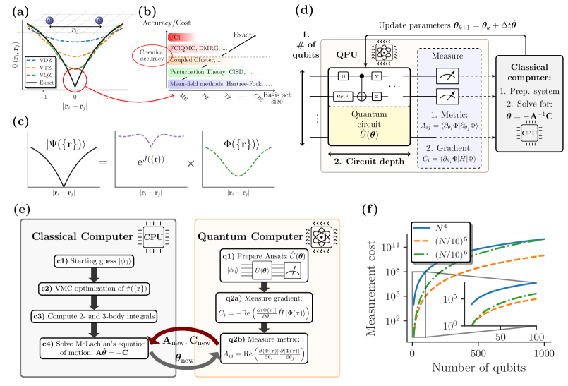
Figure 1: (a) Electron-electron cusp and increasing GTO basis set size to capture sharp features of exact groundstate wavefunction. (b) Approximate hierarchy of methods and basis set size towards exact CBS solution. (c) Jastrow Ansatz, $\ket{\Psi(\{\mathbf{r}\})}=\operatorname{e}^{\hat{J}(\{\mathbf{r}\})}\ket{\Phi(\{\mathbf{r}\})}$, capturing the sharp cusp feature with the correlator $\hat{J}(\{\mathbf{r}\})$ leaving a smoother $\ket{\Phi(\{\mathbf{r}\})}$ to solve for. (d) Hybrid quantum-classical VarQITE algorithm, where the metric, $\mathbf{A}$, and the gradient, $\mathbf{C}$, are measured on the QPU. The linear system of equations $\mathbf{A}\dot{\bm{\theta}}=-\mathbf{C}$ is solved on a classical computer to obtain new parameters $\bm{\theta}$, which are fed back to the QPU. (e) Workflow of the hybrid quantum-classical TC+VarQITE approach to solve for the right eigenvector and groundstate energy of the TC Hamiltonian $\bar{H}$. On a classical computer, we (c1) perform a conventional Hartree-Fock or MP2 calculation in a chosen basis set to obtain starting orbitals and $\ket{\phi_{0}}$. (c2) Then we optimize the Jastrow factor $\hat{J}$ with VMC (energy or reference-variance minimization) using the CASINO package[51, 52]. (c3) We compute the necessary 2- and 3-body integrals with the TCHint library[53] for the subsequent electronic structure calculation. Then we enter the hybrid quantum-classical optimization loop, sketched in (d), consisting of (q1) preparing a parametrized Ansatz and measuring the gradient (q2a) and the metric (q2b). (f) Without any cost reduction methods[54, 55, 56, 57], like Pauli grouping[58], measurements of operators containing 2-body and 3-body terms, scale as $N^{4}$ (solid blue line) and $N^{6}$ respectively, where $N$ is the number of orbitals in the basis set. The TC method reduces the number of necessary orbitals by about an order of magnitude (green dash-dotted line). Employing approximation, see Ref. [37], reduces the scaling of the TC method to the fifth power of $N$.

II Theory and Algorithms

Within the Born-Oppenheimer approximation, the molecular Hamiltonian in first quantization (in atomic units, $\hbar=\lvert e\rvert=m_{e}=4\pi\epsilon_{0}=1$) is given by

$$\hat{H}=-\sum_{i}^{n_{e}}\left(\frac{1}{2}\nabla_{i}^{2}+\sum_{a}^{N_{a}}\frac{Z_{a}}{\lvert\mathbf{r}_{i}-\mathbf{R}_{a}\rvert}\right)+\sum_{i<j}\frac{1}{\lvert\mathbf{r}_{i}-\mathbf{r}_{j}\rvert}\,.$$ (1)

In Eq.(1), $n_{e}$ is the number of electrons, $N_{a}$ the number of nuclei, $\mathbf{R}_{a}$ and $Z_{a}$ the position and atomic number of nucleus $a$, and $\mathbf{r}_{i}$ the position of electron $i$. The divergence of the Coulomb potential, $\frac{1}{r_{ij}}$, induces a sharp cusp-like feature of the exact electronic wavefunction, $\ket{\Psi_{0}(\mathbf{r})}$, at electron coalescence, $r_{ij}=\lvert\mathbf{r}_{i}-\mathbf{r}_{j}\rvert=0$[19] (Fig. 1a). This sharp feature of $\ket{\Psi_{0}(\mathbf{r})}$ is challenging to capture using basis functions based on smooth GTOs and requires the use of large basis sets for accurate quantum chemical results (Fig. 1b).

By introducing an explicit dependence on the electron-electron distances into the wavefunction via a Jastrow Ansatz [59], $\ket{\Psi}=\operatorname{e}^{\hat{J}}\ket{\Phi}$, it is possible to exactly describe the non-smooth behavior of $\ket{\Psi}$, while leaving a much smoother wavefunction, $\ket{\Phi}$, to solve for (Fig. 1c). $\hat{J}=\hat{J}(\mathbf{r}_{1},\dots,\mathbf{r}_{n})$ is an optimizable correlator depending on the positions of the electrons. The TC method [4, 3] incorporates this correlated Ansatz directly into the Hamiltonian of the system via a similarity transformation,

$$\stackrel{{\scriptstyle\text{Original:}}}{{\hat{H}\ket{\Psi}=E\ket{\Psi}}},\quad\text{with}\;\stackrel{{\scriptstyle\text{Correlated Ansatz:}}}{{\ket{\Psi}=\operatorname{e}^{\hat{J}}\ket{\Phi}}}\quad$$ (2)

$$\rightarrow\quad\stackrel{{\scriptstyle\text{Transcorrelated Problem:}}}{{\bar{H}\ket{\Phi}=E\ket{\Phi},\;\bar{H}=\operatorname{e}^{-\hat{J}}\hat{H}\operatorname{e}^{\hat{J}}}}.$$ (3)

This similarity transformation removes the Coulomb singularity of the original molecular Hamiltonian, Eq.(1),[60] and consequently increases the smoothness of the sought-after ground state wavefunction $\ket{\Phi}$.[61] For the molecular Hamiltonian (Eq. (1)) the TC Hamiltonian, $\bar{H}=\operatorname{e}^{-\hat{J}}\hat{H}\operatorname{e}^{\hat{J}}$, can be calculated exactly [34]. $\bar{H}$ possesses non-Hermitian two-body and additionally three-body interaction terms, see the Methods V.1 for more details. In our applications, we use a Drummond-Towler-Needs Jastrow factor [62, 63], which we optimize with variational Monte Carlo (VMC)[64, 65, 66] (with a scaling $n_{e}^{3}$, on conventional hardware) using the CASINO package[51, 52]. We then use the TCHint library [53] to calculate the 2- and 3-body integrals required to construct the molecular Hamiltonian in second quantization (see Fig. 1e, Methods V and the SI[67] for details).

Due to being non-Hermitian, $\bar{H}$ has different left ($\bra{\Phi^{L}_{i}}E_{i}=\bra{\Phi^{L}_{i}}\bar{H}$) and right ($\bar{H}\ket{\Phi^{R}_{i}}=E_{i}\ket{\Phi_{i}^{R}}$), eigenvector solutions, which form a bi-orthonormal basis, $\braket{\Phi_{i}^{L}}{\Phi_{j}^{R}}=\delta_{i,j}$. In this work we solve for the right ground state wavefunction, $\ket{\Phi_{0}^{R}}$, (we drop the superscript “$R$” from here on), with the QITE algorithm [41, 68, 69]. An additional benefit of the TC method is that the right ground-eigenvector of $\bar{H}$, $\ket{\Phi_{0}}$, has a more compact form compared to the non-TC ground state solution, $\ket{\Psi_{0}}$[33]. Consequently, $\ket{\Phi_{0}}$ is easier to prepare on quantum hardware with shallower circuits[30].

QITE can be recast into a hybrid quantum-classical variational form (VarQITE) [46, 70, 29] (Fig. 1d), obtained by applying McLachlan’s variational principle [71] to the imaginary-time SE,

$$\delta\lvert\lvert\left(\partial/\partial\tau+\bar{H}-E_{\tau}\right)\ket{\Phi(\tau)}\rvert\rvert=0,$$ (4)

where $\tau=it$ is imaginary time, $\lvert\lvert\ket{\Phi}\rvert\rvert=\sqrt{{\left\langle\vphantom{\Phi\Phi}\Phi\,\right|\left.\vphantom{\Phi\Phi}\Phi\right\rangle}}$ is the norm of a quantum state $\ket{\Phi}$ and $E_{\tau}=\bra{\Phi(\tau)}\bar{H}\ket{\Phi(\tau)}$ is the expected energy at time $\tau$. With a parametrized circuit Ansatz, $\hat{U}(\bm{\theta}(\tau))$, with $n_{\theta}$ parameters, to represent/approximate the target right eigenvector, $\hat{U}(\bm{\theta}(\tau))|\phi_{0}\rangle=\ket{\Phi(\tau)}$, of the TC Hamiltonian, Eq.(4) leads to a linear system of equations

$$\mathbf{A}\dot{\bm{\theta}}=-\mathbf{C}\,,$$ (5)

which is solved on a classical computer. The updated parameters are obtained from $\bm{\theta}(\tau+\Delta\tau)=\bm{\theta}(\tau)+\Delta\tau\dot{\bm{\theta}}$ for a chosen time-step, $\Delta\tau$. The vector $\mathbf{C}$ is composed of energy gradients while the matrix $\mathbf{A}$ is related to the quantum Fischer information matrix or Fubini-Study metric [72], and encodes the metric in parameter space of the Ansatz $\hat{U}(\bm{\theta})$. The VarQITE method circumvents potential parameter optimization pitfalls [72], like barren plateaus [73], by a deterministic update of the circuit parameters according to Eq.(5). Both quantities $\mathbf{C}$ and $\mathbf{A}$ in Eq. (5) are sampled from the quantum circuit. This comes at the cost of $\mathcal{O}(n_{\theta}^{2})$ circuit evaluations to measure the matrix $\mathbf{A}$ at each iteration. However, accurate approximations have been proposed, which reduce the measurement scaling to linear [72, 74], or even constant scaling [69], and it was recently shown by van Straaten and Koczor [75] that the measurement cost of the gradient will dominate for large-scale quantum chemistry applications. The implementation of the VarQITE algorithm is detailed in the MethodsV.2 section.

The evaluation of the 3-body terms of the TC Hamiltonian might raise the question of scalability, as a 3-body term requires $\mathcal{O}(N^{6})$ measurements, where $N$ is the number of basis functions/(spin-)orbitals in the basis set. However, one should consider that for an efficient implementation of the VarQITE algorithm, we don’t need an accurate evaluation of the energy (with all 3-body terms) at each iteration until convergence is reached. This can be monitored by measuring the norm of the gradient, $\mathbf{C}$, and metric, $\mathbf{A}$. Furthermore, as the TC approaches enables a faster convergence towards the basis set limit than conventional approaches, we expect an overall decrease in the number of orbitals $N$ (and thus qubits) by an order of magnitude, leading to a $\mathcal{O}[(N/10)^{6}]$ scaling, i.e., to a decrease of the pre-factor by six orders of magnitude. Overall, this implies that in the regime up to 1000 qubits, the TC method entails orders of magnitude fewer measurements than in the non-TC case (see Fig. 1f). Furthermore, recent studies [36, 66] show that scaling of the TC approach can be further reduced to $(N/10)^{5}$ (shifting the crossover far beyond 1000 qubits) or even to $(N/10)^{4}$ by approximating all 3-body with 2-body terms [76].

Concerning the VMC optimization of the Jastrow factor, this only considers occupied orbitals in the initial HF solution. Virtual orbitals, constructed, e.g., from commonly used correlation-consistent basis sets [18] are not optimized for the TC method. Following [77, 78, 79], we will therefore use pre-optimized natural orbitals (NOs) from second-order Møller-Plesset (MP2) perturbation theory calculations. In particular, orbital pre-optimization works exceptionally well in conjunction with the TC method by efficiently truncating the virtual orbital space and reducing the resource (qubit) requirements further (see the Methods sectionV.3 and the SI[67] for details). The overall workflow of the TC-VarQITE algorithm is sketched in Fig. 1e.

III Results and Discussion

We will demonstrate the advantages of the TC approaches with three applications on relatively small systems: the beryllium atom, the hydrogen molecule, and lithium hydride. If not specified differently, simulations are performed using the unitary coupled cluster singles doubles (UCCSD) Ansatz, which gives reasonable indications about the performance on the TC Ansatz compared to the non-TC one. In this study, the VarQITE algorithm is solved in matrix form (statevector simulation), implying that all gates are implemented exactly (no qubit decoherence nor gate infidelities are considered), and sampling noise is ignored. To extrapolate for future hardware calculations, we also performed TC calculation for LiH using the hardware efficient R_y Ansatz and compared the results with non-TC calculations.

III.1 Beryllium atom

Figure 2 shows all-electron TC results as a function of basis set size (number of spin-orbitals/qubits) for the beryllium atom. To achieve results within chemical accuracy compared to the CBS limit (i.e., 1 kcal/mol = 1.6 mHartree (the gray area in Fig. 2) with an FCI calculation, one would need a cc-pCvQZ basis set containing core functions and 168 spin-orbitals. Recent (approximate) explicitly correlated calculations by Schleich et al. [28], using the VQE+[2]_R12 method, achieve much more accurate results for substantially smaller basis sets. However, their results are still not within chemical accuracy with CBS results for a realistic number of spin-orbitals/qubits on near-term quantum devices. The TC method, on the other hand, enables chemically accurate results within the exact CBS limit result using only a 6-31G basis set[17] (error of 1.45 mH) needing only 18 spin-orbitals. The necessary qubit number can even be reduced further by using parity or Bravyi-Kitaev encoding[80] and symmetry-based qubit reduction (tapering)[81, 82]. This near-CBS accuracy shows the potential of utilizing an explicitly correlated method (without any approximation) in the form of the TC approach to enable near-term quantum devices to yield accurate results for relevant quantum chemical problems.

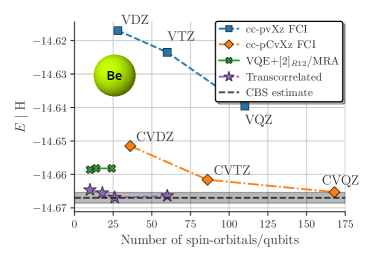
Figure 2: All-electron TC Results for the beryllium atom as a function of the number of spin-orbitals/qubits. Comparison is made with non-TC FCI results using Dunning correlation consistent basis sets with (cc-pCVxZ) and without (cc-pVxZ) core functions. Results from another explicitly correlated method, VQE+[2]_R12, developed by Schleich et al.[28] are shown for comparison. The basis sets used for TC calculations in increasing size are STO-6G, 6-31G, 6-311G, cc-pVDZ, and cc-pVTZ. Beginning with the 6-31G basis set (18 spin-orbitals/qubits), the results are within chemical accuracy (gray area) to CBS estimates[83] given by the black dashed line.

III.2 Hydrogen molecule

Figure 3a shows the energy error of TC results with respect to the CBS limit H₂ binding curve using an increasing basis set sizes/qubits. We compare our TC results with conventional FCI results in a cc-pVDZ basis set (no-TC 20 qubits) and canonical transcorrelated F12 (CT-F12)[84] results by Motta et al.[26]. The CT-F12 calculations used a 6-31G basis with eight spin-orbitals/qubits, while TC results are shown for an STO-6G (4), 6-31G (8), and cc-pvDz basis set (20 spin-orbitals/qubits respectively). Using the TC method, it is possible to almost reach chemically accurate CBS limit results (gray area in Fig. 3a) across the entire binding curve of H₂ using only a 6-31G basis set (8 spin-orbitals/qubits). We display the error statistics of the results in Fig. 3a in the form of the maximum error (MAX), the mean average error (MAE), and the non-parallelity error (NPE) in Fig. 3b. Our results show that 20 qubits (cc-pVDZ basis) are sufficient to obtain results which are on average within chemical accuracy to CBS limit results. In contrast, conventional methods require at least a cc-pVQZ basis set (120 spin-orbitals/qubits) to reach the same level of accuracy (see the SI[67]).

The improved compactness of the right eigenvector of the non-Hermitian TC Hamiltonian can be appreciated in Fig. 3c, where we report the Hartree-Fock weight, $c_{HF}$, of the original ground state wavefunction (no-TC) together with the left and right eigenvectors of the TC Hamiltonian in the cc-pVDZ basis, as a function of the bond distance. The right eigenvector has a more significant Hartree-Fock component and, thus, a single-reference character across the whole binding curve. The increase of $c_{HF}$ component is particularly pronounced in the strongly correlated dissociation regime, which is notoriously challenging for standard post-HF methods. Like for the Hubbard model studied in [30], the increased compactness results in shallower circuit Ansätze for the ground state wavefunction.

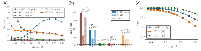
Figure 3: (a) H₂ error w.r.t. CBS limit estimates in mH vs. bond distance for TC calculations using HF orbitals in an STO-6G (4 qubits), 6-31G (8 qubits), and cc-pVDZ (20 qubits) basis set compared with no-TC FCI/cc-pVDZ calculations and CT-F12/6-31G calculations of Motta et al.[26]. (b) Error statistics (MAX, MAE, and NPE) for calculations shown in (a). (c) Hartree-Fock coefficient in the ground state wavefunction in the cc-pVDZ basis set for the original Hamiltonian (no-TC) and the left, $\bra{\Psi_{0}^{L}}$ and right, $\ket{\Psi_{0}^{R}}$, eigenvectors of the TC Hamiltonian.

III.3 Lithium hydride

Figure 4a shows the error (in mH) with respect to CBS limit estimates of TC calculations for the LiH molecule as a function of the bond distance.

We again compare with the (approximate) CT-F12 results by Motta et al. [26] and conventional FCI/cc-pVDZ results. All results in Fig. 4 are obtained with a frozen lithium 1s orbital. In addition, for the TC calculations, we used the 3 and 4 most populated MP2 natural orbitals (requiring 6 and 8 qubits, respectively) obtained with the cc-pVDZ basis, as described in the Methods section V.3. The TC method provides highly accurate energies, more accurate than the conventional FCI/cc-pVDZ results (with 38 qubits) as well as the (already quite accurate) CT-F12/6-31G approach (with 20 qubits) by Motta et al. [26]. Using only the four most occupied MP2-NOs, yields TC results essentially within chemical accuracy with respect to the CBS estimate (gray area in Fig. 4a) across the whole binding curve. The advantage of our approach is further substantiated by the statistical error analysis shown in Fig. 4b, which demonstrates how with just 3 or 4 MP2 NOs (obtained from a cc-pVDZ basis) the TC approach readily outperforms conventional methods, even when these are leveraging more orbitals. The same advantages are apparent in comparisons with other approximated, explicitly correlated approaches.

In Figure 4c, we report the HF coefficient, $c_{HF}$, of the all-electron ground state wavefunction of the original Hamiltonian (no-TC) using 14 MP2-NOs, together with the left, $\bra{\Psi_{0}^{L}}$ and right, $\ket{\Psi_{0}^{R}}$, eigenvectors of the TC Hamiltonian. Note that because the “compactification” of the right eigenvector is more pronounced for larger systems, a higher number of MP2-NOs are used. We observe that in LiH, the resulting “compactification” of the wavefunction (and corresponding circuit) is much larger than in the case of the hydrogen molecule. This increased compactness suggests an increasing benefit of the TC approach for larger systems, which exemplifies the favorable scalability of the method. With an HF coefficient greater than 0.99 over the entire dissociation profile, the TC right eigenvector can be efficiently mapped to very shallow circuits, suited for hardware calculations as shown below (see Fig. 5).

Of particular interest are the estimates for the dissociation energies reported in Figure 4d. With the TC Hamiltonian, we obtain dissociation energies of experimental accuracy with less than ten qubits, which is compatible with experiments on near-term quantum devices. In contrast, no-TC methods would require a basis set as large as cc-pVTZ, corresponding to 88 spin-orbitals, to reach comparable results, as shown in Fig. 4d.

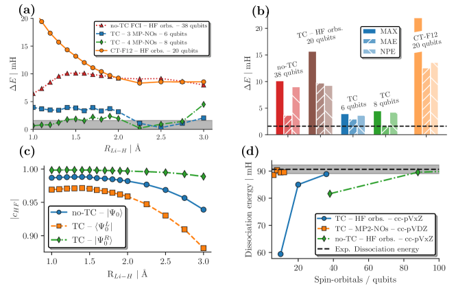
Figure 4: (a) Error of TC calculations using the three and four most occupied MP2-NOs in a cc-pVDZ basis for LiH w.r.t. CBS limit estimates in mH vs. bond distance. We compare with no-TC FCI/cc-pVDZ (38 qubits) calculations and CT-F12/6-31G (20 qubits) calculations of Motta et al.[26]. (b) MAX, MAE, and NPE values for results shown in (a). (c) Hartree-Fock coefficient, $c_{HF}$, of the all-electron ground state wavefunction using 14 MP2-NOs for the original Hamiltonian (no-TC) and the left, $\bra{\Psi_{0}^{L}}$ and right, $\ket{\Psi_{0}^{R}}$, eigenvectors of the TC Hamiltonian. (d) Dissociation energy estimates (in mH) obtained with the TC method using HF orbitals in an STO-6G, 6-31G, and cc-pVDZ basis set (blue circles), MP2 NOs (orange squares), and conventional no-TC calculations (green diamonds) as a function of the number of spin-orbitals/qubits compared to experiment[85, 86, 87] (the gray bars indicate chemical accuracy).

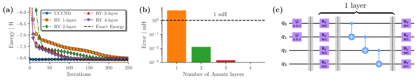
Figure 5: All-electron TC-VarQITE statevector simulations of LiH at equilibrium bond distance with 3 MP2-NOs, using the UCCSD Ansatz and a hardware-efficient RY Ansatz (c). (a) Total energy (in H) as a function of VarQITE iterations using a 1-layer UCCSD Ansatz and RY Ansätze with $1-4$ layers. (b) Error (in mH) of the RY simulations, shown in (a), w.r.t. to the TC-FCI energy as a function of the number of used layers. Two layers of the RY Ansatz suffice to obtain results within 1 mH of TC-FCI/cc-pVDZ using 3 MP2 NOs. (c) $1$-layer RY Ansatz with linear entanglement and a final rotation layer.

To further substantiate the near-term potential of our TC method, we studied the performance of a hardware-efficient Ansatz[48] and the requirements necessary to obtain energy values close to the optimal UCCSD statevector calculations described above. To this end, we performed statevector simulations for LiH at equilibrium bond distance with 3 MP2-NOs using a hardware-efficient RY Ansatz [48] with parity encoding and subsequent 2-qubit reduction (see Fig. 5c). Figure 5a shows the all-electron LiH total energy as a function of the VarQITE iterations for the UCCSD and RY Ansatz with increasing layers (up to 4). To test against robustness, we initialized the RY calculations with random parameters, while the UCCSD calculation was initialized in the HF state. The errors in the converged energies w.r.t. the exact UCCSD results using the RY Ansatz as a function of the number of Ansatz layers are shown in Figure 5b. Already two RY layers (16 single qubit R_y gates and 6 CNOT gates) suffice to obtain results within $10^{-3}$ Ha from the UCCSD reference, demonstrating the potential for near-term applications. To bring this into perspective, not even a full cc-pVDZ basis (36 qubits with parity reduction) would enable us to achieve results of this level of accuracy with conventional methods (see Fig. 4c).

Table 1: Comparison with experimental data [88, 85, 86]. We report equilibrium distances ($R_{e}$), dissociation energies ($D_{0}$), and vibrational frequencies ($\omega_{e}$) for H₂ and LiH with (TC) and without TC (no-TC). TC calculations are performed in the STO-6G basis set for H₂ and 3 MP2-NOs for LiH. For both molecules, no-TC results are obtained with STO-6G, 6-31G, and cc-pVDZ basis sets. Results by Hong et al. [89] using a Daubechies wavelet approach (denoted as DW/UCCSD) are also reported for completeness. For more details, see the SI[67].

		H2
no-TC	qubits	$R_{e}$(Å)	$D_{0}$(eV)	$\omega_{e}$(cm-1)
	4	0.73	3.67	4954
	8	0.75	3.87	4297
	20	0.76	4.19	4353
DW/UCCSD[89]	4	0.74	–	4469
TC	4	0.74	4.69	4435
Exp.		0.74	4.52	4401
		LiH
no-TC	qubits	$R_{e}$(Å)	$D_{0}$(eV)	$\omega_{e}$(cm-1)
	12	1.54	2.66	1690
	22	1.67	1.80	1283
	38	1.62	2.17	1360
DW/UCCSD[89]	10	1.61	–	1367
TC	6	1.60	2.42	1377
Exp.		1.60	2.47	1406

III.4 Comparison with experimental data

To further evaluate the quality and efficiency of the TC approach, we compare with experimental data of equilibrium bond lengths, $R_{e}$, dissociation energies, $D_{0}$, and vibrational stretching frequencies, $\omega_{e}$, for the H₂ and LiH molecules in Table 1. We note excellent agreement for all spectroscopic quantities using just four qubits for H₂ (HF orbitals in the STO-6G basis set) and six qubits for LiH (3 MP2-NOs constructed in a cc-pVDZ basis). For H₂, the TC results with four qubits yield better estimates than conventional FCI/cc-pVDZ results (20 qubits). In comparison, for LiH with 3 MP2-NOs (corresponding to 6 qubits), our TC approach readily outperforms conventional FCI/cc-pVDZresults (38 qubits).

IV Conclusions

This article describes a quantum computing implementation of an exact explicitly correlated method based on the transcorrelated approach. Unlike previous studies based on approximated TC Hamiltonians [26, 28, 31], here we consider the exact TC formalism and propose efficient theoretical and computational solutions to challenges standing in the way of its implementation as a quantum algorithm for quantum chemistry. The benefit of our approach is that it leverages the full potential of the TC method, which manifests as a dramatic cost saving (in terms of the number of qubits and gates) for current quantum hardware calculations. By incorporating the electron cusp condition, the TC method enables results within chemical accuracy and complete basis set limit results with drastically smaller basis set sizes. Because of the non-Hermitian nature of the TC Hamiltonian, standard solutions based on the variational principle, like the VQE, can not be applied for its implementation. We make use of the variational (Ansatz-based) quantum imaginary time evolution algorithm, for which recent advances [30] enable an efficient application to non-Hermitian problems. In addition, we employ a pre-optimized set of orbitals, here in the form of natural orbitals obtained from second-order Møller-Plesset perturbation theory calculations [77, 78, 79], which work exceptionally well in conjunction with the TC method, enabling a further reduction of the resources (qubits) by allowing an efficient truncation of the virtual orbital space.

The TC approach, in combination with VarQITE and orbital optimization, enables the calculation of accurate results, i.e., of nearly experimental quality, for small atomic and molecular test systems such as the beryllium atom, the hydrogen dimer, and lithium hydride, with less than 20 qubits. In particular, we were able to closely reproduce experimental values including bond lengths, dissociation energies, and the vibrational frequencies for H₂ and LiH using just 4 and 6 qubits, respectively.

In conclusion, our study demonstrates that the TC approach can become the method of choice for calculating accurate quantum chemistry observables of relevant molecular systems on near-term quantum computers. Additionally, our findings promote the use of the VarQITE algorithm for non-Hermitian problems in general, including the study of open quantum systems and transport phenomena, thus paving the way for the attainment of quantum advantage in a broader class of quantum chemistry and physics applications.

V Methods

V.1 Transcorrelation

Transcorrelation is the application of a similarity transformation to the Schrödinger equation of a system, $\hat{H}\Psi=E\Psi$, to absorb the Jastrow factor $e^{\hat{J}}$ from the ansatz $\Psi=e^{\hat{J}}\Phi$ into an effective Hamiltonian $\hat{H}_{\rm TC}=e^{-\hat{J}}\hat{H}e^{\hat{J}}$. The resulting TC Schrödinger equation, $\hat{H}_{\rm TC}\Phi=E\Phi$, can be solved in second quantization using any quantum chemistry eigensolver, including quantum computers, with the advantage that the FCI solution for $\Phi$ is much more compact than that for $\Psi$, and thus easier to represent approximately. Eigensolvers only require the values of the matrix elements of ${\hat{H}}_{\rm TC}$ between different determinants. If the Jastrow factor can be written as $J=\sum_{i<j}u({\bf r}_{i},{\bf r}_{j})$ then

$$\hat{H}_{\rm TC}=\hat{H}-\sum_{i<j}\hat{K}({\bf r}_{i},{\bf r}_{j})-\sum_{i<j<k}\hat{L}({\bf r}_{i},{\bf r}_{j},{\bf r}_{k})\;,$$ (6)

where $\hat{K}$ is an operator that modifies the values of two-electron matrix elements and introduces non-Hermiticity and $\hat{L}$ is an operator that connects determinants separated by triple excitations. Eigensolvers thus need the ability to accommodate non-Hermiticity and three-electron matrix elements, so non-TC implementations usually require some degree of modification.

We use a Drummond-Towler-Needs Jastrow factor [62, 63], which we optimize with VMC[66] using the CASINO package[51, 52]. We then use the TCHint library [53] to calculate the 2- and 3-body integrals required to construct the molecular Hamiltonian in second quantization. See Ref. [[66]] and the SI[67] for more details and sample input files of the VMC optimization and integral calculation.

V.2 Variational Ansatz-based quantum imaginary time evolution

The VarQITE algorithm [70] is based on McLachlan’s variational principle, which is used to derive the evolution of gate parameters, represented by $\bm{\theta}(\tau)$, for a wavefunction Ansatz. The derivation is encapsulated in Eq. (4), which leads to a linear system of equations defined in Eq. (5). This system necessitates the computation of matrix elements associated with the matrix $\mathbf{A}$ and the gradient vector $\mathbf{C}$ defined as

$$A_{ij} =\text{Re}\left(\frac{\partial\bra{\Phi(\bm{\theta}(\tau))}}{\partial\theta_{i}}\frac{\partial\ket{\Phi(\bm{\theta}(\tau))}}{\partial\theta_{j}}\right)\,,$$ (7)

and

$$C_{i}= \text{Re}\left(\frac{\partial\bra{\Phi(\bm{\theta}(\tau))}}{\partial\theta_{i}}\hat{H}\ket{\Phi(\bm{\theta}(\tau))}\right),$$ (8)

where the wavefunction Ansatz is differentiated with respect to the gate parameters. In our implementation, their calculation is performed using the methodology outlined in [30], specifically designed for non-Hermitian (TC) problems. Next, we give more details about the steps necessary to reproduce the results of this work.

In numerical simulations, the values of $A_{ij}$ and $C_{i}$ are estimated using the forward finite-differences method [90] given by

$$\frac{\partial\ket{\Phi(\bm{\theta})}}{\partial\theta_{j}}\approx\frac{\ket{\Phi(\bm{\theta}+\Delta\mathbb{\hat{e}}_{j})}-\ket{\Phi(\bm{\theta})}}{\Delta},$$ (9)

where $\mathbb{\hat{e}}_{j}$ is $j$-th element of the $n_{\theta}$-dimensional unit vector and we chose a step-size of $\Delta=10^{-3}$ in this work. To generate the state-vector representation of the Ansatz $\ket{\Phi(\bm{\theta})}$, we create the corresponding quantum circuit in Qiskit [91] and then convert it to a state-vector. This approach allows for the incorporation of gate errors through realistic noise models of IBM Quantum processors. The matrix elements $A_{ij}$ and $C_{i}$ can be computed independently, and we parallelize their computation on multiple CPUs using the ipyparallel library to speed up our simulations. Although the forward finite-differences method provides satisfactory results for the computation of the derivatives, the parameter-shift rule [92] can also be employed within our framework to obtain analytic derivatives.

In hardware calculations, the matrix elements $A_{ij}$ and $C_{i}$ are calculated via the differentiation of general gates by means of a linear combination of unitaries [92]. To compute the $C_{i}$ elements, we use a quantum circuit (Fig. 6) with $V$ being a Hadamard gate (H) for a Hermitian Hamiltonian. For a non-Hermitian Hamiltonian, $\bar{H}$, we decompose $\bar{H}$ into hermitian and anti-hermitian components denoted by $\bar{H}=(\hat{H}^{+}+\hat{H}^{-})/2$, where $\hat{H}^{+}=\bar{H}+\bar{H}^{\dagger}$ and $\hat{H}^{-}=\bar{H}-\bar{H}^{\dagger}$. Subsequently, the circuit from Fig. 6 is applied to each term of $\hat{H}^{+}$ and $\hat{H}^{-}$, utilizing the adapted version of the $V$ gate specified in the legend of Fig. 6. The measurement outcomes obtained from this circuit are then combined to obtain $C_{i}$ as in Refs. [92, 30]. To compute the $A_{ij}$ matrix elements we proceed in the standard way, which can be found in Refs. [21], since they are independent of the Hamiltonian. We typically use $10^{4}$ to $3.2\cdot 10^{4}$ shots (measurements) to collect enough statistics for accurate estimates of the expectation values.

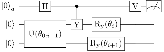
Figure 6: Quantum circuit used to calculate the $C_{i}$ term in the (non-)Hermitian case for a (TC) Hamiltonian. A Hamiltonian is first separated into its Hermitian and anti-Hermitian parts. The circuit uses the Hadamard gate $V=H$ for the Hermitian part, and the gate $V=R_{x}(\frac{\pi}{2})$ for the anti-Hermitian part. This circuit needs to be repeated for every term in a Hamiltonian.

For the representations of Ansatz circuits, we use Qiskit’s implementation of UCCSD and hardware-efficient Ansätze with the default settings.

Having all the necessary quantities, the linear system in Eq. (5), can be approximately inverted to obtain $\dot{\bm{\theta}}=-\mathbf{A}^{-1}\mathbf{C}\,$ using the least-square solver (default settings) implemented in SciPy [93]. Finally, the updated parameters are obtained from $\bm{\theta}(\tau+\Delta\tau)=\bm{\theta}(\tau)+\Delta\tau\dot{\bm{\theta}}$ for a chosen time-step of $\Delta\tau=0.05$ in this work. We studied the stability and convergence properties of VarQITE w.r.t. different values of $\Delta\tau$ including the resilience to simulated hardware noise, see the SI[67].

V.3 MP2 – NOs

The 1-body reduced density matrix (1-RDM) in a second-quantized basis is defined as

$$D^{p}_{q}=\braket{\Psi}{\hat{a}^{\dagger}_{p}\hat{a}_{q}}{\Psi},$$ (10)

where $\ket{\Psi}$ is the wavefunction and $p,q$ refer to the indices of the current basis. The diagonalization of Eq. (10) provides the eigenvalues as the occupation numbers and the eigenvectors as the transformation matrix from the current basis to the natural orbital basis. Löwdin [94] first used NOs to accelerate the convergence with respect to the basis set in configuration interaction theory by retaining only those NOs with significantly nonzero occupation numbers. The specific natural orbitals used in this work are obtained at the MP2 level. First, a mean-field HF solution to the system under study is obtained in a reasonably large basis set, e.g., cc-pVDZ or cc-pVTZ, and in the HF canonical orbital basis. The MP2 wavefunction is

$$\ket{\Psi_{\rm MP2}}=\ket{\Psi_{\rm HF}}+\sum_{i>j,a>b}\frac{\braket{ab}{ij}}{\Delta^{ab}_{ij}}\ket{\Psi^{ab}_{ij}},$$ (11)

where we follow convention to use $a,b,\dots$ and $i,j,\dots$ to indicate the unoccupied (virtual) and occupied spin-orbitals, respectively; the antisymmetrized Coulomb integrals are defined as $\braket{ab}{ij}=\braket{ab}{ij}-\braket{ab}{ji}$ and the denominator is $\Delta^{ab}_{ij}=\varepsilon_{i}+\varepsilon_{j}-\varepsilon_{a}-\varepsilon_{b}$ with $\varepsilon_{i}$ being the orbital energies (diagonal elements of the Fock matrix).

Plugging $\ket{\Psi_{\rm MP2}}$ into Eq. (10), we find

$$D^{i}_{j} =\delta_{i,j}+\frac{1}{2}\sum_{kab}\frac{\braket{ki}{ab}\braket{ab}{kj}}{\Delta^{ab}_{ki}\Delta^{ab}_{kj}},$$ (12)

$$D^{a}_{b} =\frac{1}{2}\sum_{ijc}\frac{\braket{ij}{ac}\braket{bc}{ij}}{\Delta^{ac}_{ij}\Delta^{bc}_{ij}},$$

where following the PySCF[95] standard, we ignore orbital rotations between the occupied and virtual space by setting the occupied-virtual block $D^{a}_{i}=D^{i}_{a}=0$. In literature, the so-called frozen natural orbitals (FNO) are obtained by only diagonalizing the virtual-virtual block of the 1-RDM $D^{a}_{b}$. In this work, we diagonalize both the occupied-occupied and virtual-virtual blocks.

For more details on the used MP2-NOs for the LiH calculations and a sample PySCF[95] script to generate them, see the SI[67].

VI End notes

VI.1 Acknowledgments

Funded by the European Union. Views and opinions expressed are, however, those of the author(s) only and do not necessarily reflect those of the European Union or REA. Neither the European Union nor the granting authority can be held responsible for them. This project has received funding from the European Union’s Horizon Europe research and innovation programme under the Marie Skłodowska-Curie grant agreement No. 101062864. IT acknowledges funding from the NCCR MARVEL, a National Centre of Competence in Research by the Swiss National Science Foundation (grant number 205602). This research has been supported by funding from the Wallenberg Center for Quantum Technology (WACQT). This research relied on computational resources provided by the Swedish National Infrastructure for Computing (SNIC) at C3SE, NSC, and PDC, partially funded by the Swedish research council through grant agreement no 2018-05973. We acknowledge the use of IBM Quantum services for this work. The views expressed are those of the authors and do not reflect the official policy or position of IBM or the IBM Quantum team. IBM, the IBM logo, and ibm.com are trademarks of International Business Machines Corp., registered in many jurisdictions worldwide. Other product and service names might be trademarks of IBM or other companies. The current list of IBM trademarks is available at https://www.ibm.com/legal/copytrade.

The authors declare no competing interests.

VI.2 Additional Information

Supplementary Information is available for this paper.[67] Correspondence and requests for materials should be addressed to Werner Dobrautz, dobrautz@chalmers.se.

References

- Benioff [1980] P. Benioff, J. Statist. Phys. 22, 563 (1980).
- Feynman [1982] R. P. Feynman, Int. J. Theor. Phys. 21 (1982).
- Boys and Handy [1969a] S. Boys and N. Handy, Proc. R. Soc. Lond. A 309, 209 (1969a).
- Boys and Handy [1969b] S. Boys and N. Handy, Proc. R. Soc. Lond. A 310, 43 (1969b).
- Boys and Handy [1969c] S. Boys and N. Handy, Proc. R. Soc. Lond. A 310, 63 (1969c).
- Helgaker et al. [2000] T. Helgaker, P. Jørgensen, and J. Olsen, Molecular Electronic-Structure Theory (Wiley, 2000).
- Bednorz and Müller [1986] J. G. Bednorz and K. A. Müller, Z. Phys. B 64, 189 (1986).
- Renger [1987] G. Renger, Angew. Chem. (International) 26, 643 (1987).
- Mukhopadhyay et al. [2004] S. Mukhopadhyay, S. K. Mandal, S. Bhaduri, and W. H. Armstrong, Chem. Rev. 104, 3981 (2004).
- Holm et al. [1996] R. H. Holm, P. Kennepohl, and E. I. Solomon, Chem. Rev. 96, 2239 (1996).
- Stappen et al. [2020] C. V. Stappen, L. Decamps, G. E. Cutsail, R. Bjornsson, J. T. Henthorn, J. A. Birrell, and S. DeBeer, Chem. Rev. 120, 5005 (2020).
- White [1992] S. R. White, Phys. Rev. Lett. 69, 2863 (1992).
- Čížek [1966] J. Čížek, J. Chem. Phys. 45, 4256 (1966).
- Nightingale and Umrigar [1998] M. Nightingale and C. J. Umrigar, Quantum Monte Carlo Methods in Physics and Chemistry (Springer Dordrecht, 1998).
- Becca and Sorella [2017] F. Becca and S. Sorella, Quantum Monte Carlo Approaches for Correlated Systems (Cambridge University Press, 2017).
- Boys [1950] S. F. Boys, Proc. R. Soc. Lond. A 200, 542 (1950).
- Ditchfield et al. [1971] R. Ditchfield, W. J. Hehre, and J. A. Pople, J. Chem. Phys. 54, 724 (1971).
- Dunning [1989] T. H. Dunning, J. Chem. Phys. 90, 1007 (1989).
- Kato [1957] T. Kato, Commun. Pure Appl. Math. 10, 151 (1957).
- Nielsen and Chuang [2012] M. A. Nielsen and I. L. Chuang, Quantum Computation and Quantum Information (Cambridge University Press, 2012).
- McArdle et al. [2020] S. McArdle, S. Endo, A. Aspuru-Guzik, S. C. Benjamin, and X. Yuan, Rev. Mod. Phys. 92, 015003 (2020).
- Bauer et al. [2020] B. Bauer, S. Bravyi, M. Motta, and G. K.-L. Chan, Chem. Rev. 120, 12685 (2020).
- Eddins et al. [2022] A. Eddins, M. Motta, T. P. Gujarati, S. Bravyi, A. Mezzacapo, C. Hadfield, and S. Sheldon, PRX Quantum 3, 010309 (2022).
- Lee et al. [2021] J. Lee, D. W. Berry, C. Gidney, W. J. Huggins, J. R. McClean, N. Wiebe, and R. Babbush, PRX Quantum 2, 030305 (2021).
- Motta et al. [2021] M. Motta, E. Ye, J. R. McClean, Z. Li, A. J. Minnich, R. Babbush, and G. K.-L. Chan, npj Quantum Inf. 7, 10.1038/s41534-021-00416-z (2021).
- Motta et al. [2020] M. Motta, T. P. Gujarati, J. E. Rice, A. Kumar, C. Masteran, J. A. Latone, E. Lee, E. F. Valeev, and T. Y. Takeshita, Phys. Chem. Chem. Phys. 22, 24270 (2020).
- Kottmann et al. [2021] J. S. Kottmann, P. Schleich, T. Tamayo-Mendoza, and A. Aspuru-Guzik, J. Phys. Chem. Lett. 12, 663 (2021).
- Schleich et al. [2021] P. Schleich, J. S. Kottmann, and A. Aspuru-Guzik, arXiv preprint arXiv:2110.06812 (2021).
- McArdle and Tew [2020] S. McArdle and D. P. Tew, arXiv preprint arXiv:2006.11181 (2020).
- Sokolov et al. [2022] I. O. Sokolov, W. Dobrautz, H. Luo, A. Alavi, and I. Tavernelli, (2022), arXiv:2201.03049 [quant-ph] .
- Kumar et al. [2022] A. Kumar, A. Asthana, C. Masteran, E. F. Valeev, Y. Zhang, L. Cincio, S. Tretiak, and P. A. Dub, J. Chem. Theory Comput. 18, 5312 (2022).
- Kutzelnigg [1985] W. Kutzelnigg, Theor. Chim. Acta 68, 445 (1985).
- Dobrautz et al. [2019] W. Dobrautz, H. Luo, and A. Alavi, Phys. Rev. B 99, 075119 (2019).
- Cohen et al. [2019] A. J. Cohen, H. Luo, K. Guther, W. Dobrautz, D. P. Tew, and A. Alavi, J. Chem. Phys. 151, 061101 (2019).
- Guther et al. [2021] K. Guther, A. J. Cohen, H. Luo, and A. Alavi, J. Chem. Phys. 155, 011102 (2021).
- Dobrautz et al. [2022] W. Dobrautz, A. J. Cohen, A. Alavi, and E. Giner, J. Chem. Phys. 156, 234108 (2022).
- Giner [2021] E. Giner, J. Chem. Phys. 154, 084119 (2021).
- Peruzzo et al. [2014] A. Peruzzo, J. McClean, P. Shadbolt, M.-H. Yung, X.-Q. Zhou, P. J. Love, A. Aspuru-Guzik, and J. L. O’brien, Nat. Commun. 5, 4213 (2014).
- McClean et al. [2016] J. R. McClean, J. Romero, R. Babbush, and A. Aspuru-Guzik, New J. Phys. 18, 023023 (2016).
- Cerezo et al. [2021] M. Cerezo, A. Arrasmith, R. Babbush, S. C. Benjamin, S. Endo, K. Fujii, J. R. McClean, K. Mitarai, X. Yuan, L. Cincio, and P. J. Coles, Nat. Rev. Phys. 3, 625 (2021).
- Motta et al. [2019] M. Motta, C. Sun, A. T. K. Tan, M. J. O’Rourke, E. Ye, A. J. Minnich, F. G. S. L. Brandão, and G. K.-L. Chan, Nat. Phys. 16, 205 (2019).
- Gomes et al. [2020] N. Gomes, F. Zhang, N. F. Berthusen, C.-Z. Wang, K.-M. Ho, P. P. Orth, and Y. Yao, J. Chem. Theory Comput. 16, 6256 (2020).
- Cao et al. [2022] C. Cao, Z. An, S.-Y. Hou, D. L. Zhou, and B. Zeng, Communications Physics 5, 10.1038/s42005-022-00837-y (2022).
- Nishi et al. [2021] H. Nishi, T. Kosugi, and Y. ichiro Matsushita, npj Quantum Inf. 7, 10.1038/s41534-021-00409-y (2021).
- Tsuchimochi et al. [2023] T. Tsuchimochi, Y. Ryo, S. L. Ten-no, and K. Sasasako, Journal of Chemical Theory and Computation 10.1021/acs.jctc.2c00906 (2023).
- Yuan et al. [2019] X. Yuan, S. Endo, Q. Zhao, Y. Li, and S. C. Benjamin, Quantum 3, 191 (2019).
- Google AI Quantum et al. [2020] Google AI Quantum, F. Arute, K. Arya, R. Babbush, D. Bacon, J. C. Bardin, R. Barends, S. Boixo, M. Broughton, B. B. Buckley, D. A. Buell, B. Burkett, N. Bushnell, Y. Chen, Z. Chen, B. Chiaro, R. Collins, W. Courtney, S. Demura, A. Dunsworth, E. Farhi, A. Fowler, B. Foxen, C. Gidney, M. Giustina, R. Graff, S. Habegger, M. P. Harrigan, A. Ho, S. Hong, T. Huang, W. J. Huggins, L. Ioffe, S. V. Isakov, E. Jeffrey, Z. Jiang, C. Jones, D. Kafri, K. Kechedzhi, J. Kelly, S. Kim, P. V. Klimov, A. Korotkov, F. Kostritsa, D. Landhuis, P. Laptev, M. Lindmark, E. Lucero, O. Martin, J. M. Martinis, J. R. McClean, M. McEwen, A. Megrant, X. Mi, M. Mohseni, W. Mruczkiewicz, J. Mutus, O. Naaman, M. Neeley, C. Neill, H. Neven, M. Y. Niu, T. E. O’Brien, E. Ostby, A. Petukhov, H. Putterman, C. Quintana, P. Roushan, N. C. Rubin, D. Sank, K. J. Satzinger, V. Smelyanskiy, D. Strain, K. J. Sung, M. Szalay, T. Y. Takeshita, A. Vainsencher, T. White, N. Wiebe, Z. J. Yao, P. Yeh, and A. Zalcman, Science 369, 1084 (2020).
- Kandala et al. [2017] A. Kandala, A. Mezzacapo, K. Temme, M. Takita, M. Brink, J. M. Chow, and J. M. Gambetta, Nature 549, 242 (2017).
- Nam et al. [2020] Y. Nam, J.-S. Chen, N. C. Pisenti, K. Wright, C. Delaney, D. Maslov, K. R. Brown, S. Allen, J. M. Amini, J. Apisdorf, K. M. Beck, A. Blinov, V. Chaplin, M. Chmielewski, C. Collins, S. Debnath, K. M. Hudek, A. M. Ducore, M. Keesan, S. M. Kreikemeier, J. Mizrahi, P. Solomon, M. Williams, J. D. Wong-Campos, D. Moehring, C. Monroe, and J. Kim, npj Quantum Inf. 6, 10.1038/s41534-020-0259-3 (2020).
- ibm [2022] https://www.ibm.com/quantum/roadmap (2022).
- Needs et al. [2020] R. J. Needs, M. D. Towler, N. D. Drummond, P. L. Ríos, and J. R. Trail, J. Chem. Phys. 152, 154106 (2020).
- López Ríos et al. [2006] P. López Ríos, A. Ma, N. D. Drummond, M. D. Towler, and R. J. Needs, Phys. Rev. E 74, 066701 (2006).
- López Ríoz and et al. [2023] P. López Ríoz and et al. (2023), to be published.
- Yen et al. [2020] T.-C. Yen, V. Verteletskyi, and A. F. Izmaylov, J. Chem. Theory Comput. 16, 2400 (2020).
- Verteletskyi et al. [2020] V. Verteletskyi, T.-C. Yen, and A. F. Izmaylov, J. Chem. Phys. 152, 124114 (2020).
- Yen and Izmaylov [2021] T.-C. Yen and A. F. Izmaylov, PRX Quantum 2, 040320 (2021).
- Izmaylov et al. [2019a] A. F. Izmaylov, T.-C. Yen, R. A. Lang, and V. Verteletskyi, J. Chem. Theory Comput. 16, 190 (2019a).
- Izmaylov et al. [2019b] A. F. Izmaylov, T.-C. Yen, and I. G. Ryabinkin, Chem. Sci. 10, 3746 (2019b).
- Jastrow [1955] R. Jastrow, Phys. Rev. 98, 1479 (1955).
- Luo and Alavi [2018] H. Luo and A. Alavi, J. Chem. Theory Comput. 14, 1403 (2018).
- Fournais et al. [2005] S. Fournais, M. Hoffmann-Ostenhof, T. Hoffmann-Ostenhof, and T. Ø. Sørensen, Comm. Math. Phys. 255, 183 (2005).
- Drummond et al. [2004] N. D. Drummond, M. D. Towler, and R. J. Needs, Phys. Rev. B 70, 235119 (2004).
- López Ríos et al. [2012] P. López Ríos, P. Seth, N. D. Drummond, and R. J. Needs, Phys. Rev. E 86, 036703 (2012).
- Ceperley et al. [1977] D. Ceperley, G. V. Chester, and M. H. Kalos, Phys. Rev. B 16, 3081 (1977).
- Foulkes et al. [2001] W. M. C. Foulkes, L. Mitas, R. J. Needs, and G. Rajagopal, Rev. Mod. Phys. 73, 33 (2001).
- Haupt et al. [2023] J. P. Haupt, S. M. Hosseini, P. L. Rios, W. Dobrautz, A. Cohen, and A. Alavi, (2023), arXiv:2302.13683 [physics.chem-ph] .
- SI [2023] (2023), supplementary material is available at: To be added by publisher.
- Zoufal et al. [2021] C. Zoufal, D. Sutter, and S. Woerner, (2021), arXiv:2108.00022 [quant-ph] .
- Gacon et al. [2021] J. Gacon, C. Zoufal, G. Carleo, and S. Woerner, Quantum 5, 567 (2021).
- McArdle et al. [2019] S. McArdle, T. Jones, S. Endo, Y. Li, S. C. Benjamin, and X. Yuan, npj Quantum Inf. 5, 1 (2019).
- McLachlan [1964] A. McLachlan, Mol. Phys. 8, 39 (1964).
- Stokes et al. [2020] J. Stokes, J. Izaac, N. Killoran, and G. Carleo, Quantum 4, 269 (2020).
- McClean et al. [2018] J. R. McClean, S. Boixo, V. N. Smelyanskiy, R. Babbush, and H. Neven, Nat. Commun. 9, 10.1038/s41467-018-07090-4 (2018).
- Fitzek et al. [2023] D. Fitzek, R. Jonsson, W. Dobrautz, and C. Schäfer (2023), to be published.
- van Straaten and Koczor [2021] B. van Straaten and B. Koczor, PRX Quantum 2, 030324 (2021).
- Chrislmaier and et al. [2023] E. Chrislmaier and et al. (2023), to be published.
- Kühn et al. [2019] M. Kühn, S. Zanker, P. Deglmann, M. Marthaler, and H. Weiß, J. Chem. Theory Comput. 15, 4764 (2019).
- Verma et al. [2021] P. Verma, L. Huntington, M. P. Coons, Y. Kawashima, T. Yamazaki, and A. Zaribafiyan, J. Chem. Phys. 155, 034110 (2021).
- Gonthier et al. [2022] J. F. Gonthier, M. D. Radin, C. Buda, E. J. Doskocil, C. M. Abuan, and J. Romero, Phys. Rev. Research 4, 033154 (2022).
- Bravyi and Kitaev [2002] S. B. Bravyi and A. Y. Kitaev, Ann. Physics 298, 210 (2002).
- Setia et al. [2020] K. Setia, R. Chen, J. E. Rice, A. Mezzacapo, M. Pistoia, and J. D. Whitfield, J. Chem. Theory Comput. 16, 6091 (2020).
- Bravyi et al. [2017] S. Bravyi, J. M. Gambetta, A. Mezzacapo, and K. Temme, (2017), arXiv:1701.08213 [quant-ph] .
- Davidson et al. [1991] E. R. Davidson, S. A. Hagstrom, S. J. Chakravorty, V. M. Umar, and C. F. Fischer, Phys. Rev. A 44, 7071 (1991).
- Yanai and Shiozaki [2012] T. Yanai and T. Shiozaki, J. Chem. Phys. 136, 084107 (2012).
- Stwalley and Zemke [1993] W. C. Stwalley and W. T. Zemke, J. Phys. Chem. Ref. Data 22, 87 (1993).
- Haeffler et al. [1996] G. Haeffler, D. Hanstorp, I. Kiyan, A. E. Klinkmüller, U. Ljungblad, and D. J. Pegg, Phys. Rev. A 53, 4127 (1996).
- Rumble [2022] J. Rumble, ed., CRC handbook of chemistry and physics, 103rd ed., CRC Handbook of Chemistry and Physics (Taylor & Francis, London, England, 2022).
- Huber and Herzberg [1979] K. P. Huber and G. Herzberg, in Molecular Spectra and Molecular Structure (Springer US, 1979) pp. 8–689.
- Hong et al. [2022] C.-L. Hong, T. Tsai, J.-P. Chou, P.-J. Chen, P.-K. Tsai, Y.-C. Chen, E.-J. Kuo, D. Srolovitz, A. Hu, Y.-C. Cheng, and H.-S. Goan, PRX Quantum 3, 020360 (2022).
- Milne-Thomson [2000] L. M. Milne-Thomson, The calculus of finite differences (American Mathematical Soc., 2000).
- Aleksandrowicz et al. [2019] G. Aleksandrowicz, T. Alexander, P. Barkoutsos, L. Bello, Y. Ben-Haim, D. Bucher, F. J. Cabrera-Hernández, J. Carballo-Franquis, A. Chen, C.-F. Chen, J. M. Chow, A. D. Córcoles-Gonzales, A. J. Cross, A. Cross, J. Cruz-Benito, C. Culver, S. D. L. P. González, E. D. L. Torre, D. Ding, E. Dumitrescu, I. Duran, P. Eendebak, M. Everitt, I. F. Sertage, A. Frisch, A. Fuhrer, J. Gambetta, B. G. Gago, J. Gomez-Mosquera, D. Greenberg, I. Hamamura, V. Havlicek, J. Hellmers, Łukasz Herok, H. Horii, S. Hu, T. Imamichi, T. Itoko, A. Javadi-Abhari, N. Kanazawa, A. Karazeev, K. Krsulich, P. Liu, Y. Luh, Y. Maeng, M. Marques, F. J. Martín-Fernández, D. T. McClure, D. McKay, S. Meesala, A. Mezzacapo, N. Moll, D. M. Rodríguez, G. Nannicini, P. Nation, P. Ollitrault, L. J. O’Riordan, H. Paik, J. Pérez, A. Phan, M. Pistoia, V. Prutyanov, M. Reuter, J. Rice, A. R. Davila, R. H. P. Rudy, M. Ryu, N. Sathaye, C. Schnabel, E. Schoute, K. Setia, Y. Shi, A. Silva, Y. Siraichi, S. Sivarajah, J. A. Smolin, M. Soeken, H. Takahashi, I. Tavernelli, C. Taylor, P. Taylour, K. Trabing, M. Treinish, W. Turner, D. Vogt-Lee, C. Vuillot, J. A. Wildstrom, J. Wilson, E. Winston, C. Wood, S. Wood, S. Wörner, I. Y. Akhalwaya, and C. Zoufal, Qiskit: An Open-source Framework for Quantum Computing (2019).
- Schuld et al. [2019] M. Schuld, V. Bergholm, C. Gogolin, J. Izaac, and N. Killoran, Phys. Rev. A 99, 032331 (2019).
- Virtanen et al. [2020] P. Virtanen, R. Gommers, T. E. Oliphant, M. Haberland, T. Reddy, D. Cournapeau, E. Burovski, P. Peterson, W. Weckesser, J. Bright, S. J. van der Walt, M. Brett, J. Wilson, K. J. Millman, N. Mayorov, A. R. J. Nelson, E. Jones, R. Kern, E. Larson, C. J. Carey, İ. Polat, Y. Feng, E. W. Moore, J. VanderPlas, D. Laxalde, J. Perktold, R. Cimrman, I. Henriksen, E. A. Quintero, C. R. Harris, A. M. Archibald, A. H. Ribeiro, F. Pedregosa, P. van Mulbregt, and SciPy 1.0 Contributors, Nat. Methods 17, 261 (2020).
- Löwdin [1955] P.-O. Löwdin, Phys. Rev. 97, 1474 (1955).
- Sun et al. [2020] Q. Sun, X. Zhang, S. Banerjee, P. Bao, M. Barbry, N. S. Blunt, N. A. Bogdanov, G. H. Booth, J. Chen, Z.-H. Cui, J. J. Eriksen, Y. Gao, S. Guo, J. Hermann, M. R. Hermes, K. Koh, P. Koval, S. Lehtola, Z. Li, J. Liu, N. Mardirossian, J. D. McClain, M. Motta, B. Mussard, H. Q. Pham, A. Pulkin, W. Purwanto, P. J. Robinson, E. Ronca, E. R. Sayfutyarova, M. Scheurer, H. F. Schurkus, J. E. T. Smith, C. Sun, S.-N. Sun, S. Upadhyay, L. K. Wagner, X. Wang, A. White, J. D. Whitfield, M. J. Williamson, S. Wouters, J. Yang, J. M. Yu, T. Zhu, T. C. Berkelbach, S. Sharma, A. Y. Sokolov, and G. K.-L. Chan, The Journal of Chemical Physics 153, 024109 (2020).