Mean-field criticality explained by random matrices theory

Abstract

How a system initially at infinite temperature responds when suddenly placed at finite temperatures is a way to check the existence of phase transitions. It has been shown in [R. da Silva, IJMPC 2023] that phase transitions are imprinted in the spectra of matrices built from time evolutions of magnetization of spin models. In this paper, we show that this method works very accurately in determining the critical temperature in the mean-field Ising model. We show that for Glauber or Metropolis dynamics, the average eigenvalue has a minimum at the critical temperature, which is corroborated by an inflection at eigenvalue dispersion at this same point. Such transition is governed by a gap in the density of eigenvalues similar to short-range spin systems. We conclude that the thermodynamics of this mean-field system can be described by the fluctuations in the spectra of Wishart matrices which suggests a direct relationship between thermodynamic fluctuations and spectral fluctuations.

1 Introduction

Ising-like Hamiltonians Salinas can be simply written as:

$$\mathcal{H}=-J\sum\limits_{\left\langle i,j\right\rangle}s_{i}s_{j}-h\sum\limits_{i=1}^{N}s_{i}\,,$$ (1)

where $s_{i}=\pm 1$ (spin 1/2). Here $h$ is the external field that couples with each spin, and $\left\langle i,j\right\rangle$ denotes the sum over the nearest neighbors in a $d$-dimensional lattice. Each spin, placed in its original lattice, is linked to other $z=2^{d}$ neighbors. The number of links in the lattice is $\frac{Nz}{2}$ where factor 1/2 avoids double counting.

A mean-field (MF) approximation considers that each spin $s_{i}$ interacts with a kind of magnetic cloud represented (composed?) by the average magnetization of all other spins, that is: $\xi_{i}=$ $\frac{1}{N}\sum\limits_{j=1,j\neq i}^{N}s_{j}$. Thus, in this approximation, the interacting term $H_{int}=-J\sum\limits_{\left\langle i,j\right\rangle}s_{i}s_{j}$ must be replaced by

$$\mathcal{H}_{int}^{(MF)}=-\frac{Jz}{2}\sum\limits_{i=1}^{N}s_{i}\xi_{i}\approx-\frac{Jz}{2N}\sum\limits_{i=1}^{N}\sum\limits_{j=1}^{N}s_{i}s_{j}.$$

Finally, one has that mean-field Hamiltonian is given by

$$\mathcal{H}^{(MF)}=-\frac{Jz}{2N}M^{2}-hM\text{,}$$ (2)

where $M=\sum\limits_{i=1}^{N}s_{i}$ is the total magnetization of the system. Its properties are well known and, once our interest is in its behavior close to the continuous phase transition at $\beta_{c}zJ=1$, the external field $h$ is made null in this work.

To briefly contextualize, the long-range (LR) MF regime has been explored in several models Wreszinski . It has been also shown that Monte Carlo (MC) simulations could be applied to the MF Ising Model Henriques ; Drugowich-Libero .

When dealing with equilibrium properties, we can choose any prescription for system’s dynamics that satisfies the detailed balance condition, for example, the usual Glauber dynamics for a single spin flip, $s_{i}\to-s_{i}$:

$$w(s\rightarrow s^{(j)})=\frac{1}{2\tau}\left[1-\tanh\left(\beta\frac{\Delta\mathcal{H}^{(MF)}}{2}\right)\right]$$ (3)

where $\tau$ is a characteristic parameter that can be made equal to one or fitted to the time scale of the specific problem, $\beta=1/(k_{B}T)$ is the inverse of temperature ($T$) and $\Delta\mathcal{H}^{(MF)}$ is system’s energy change due to the flip of spin $s_{i}$.

In the case of the MF Ising model, one has $\Delta\mathcal{H}^{(MF)}=-\frac{J}{2N}z\left[\left(\sum_{i=1,\ i\neq j}^{N}s_{i}-s_{j}\right)^{2}-\left(\sum_{i=1,\ i\neq j}^{N}s_{i}+s_{j}\right)^{2}\right]=\frac{2J}{N}zs_{j}\left(M-s_{j}\right)\approx\frac{2J}{N}zs_{j}M$ . Thus, since $s_{j}^{2}=1$, $\left\langle s_{j}\right\rangle=m$, and considering that in the MF one has$\ \left\langle\tanh\left(\frac{\beta J}{N}zM\right)\right\rangle=\tanh\left\langle\frac{\beta J}{N}zM\right\rangle=\tanh(\beta zJm)$. With these quantities, it is possible to write the time evolution of magnetization MarioBook

$$\tau\frac{dm}{dt}=-m+\tanh{(\beta Jzm)}$$ (4)

where $m=\lim_{N\rightarrow\infty}\frac{\left\langle M\right\rangle}{N}$. One should note that the RHS of this equation is exactly the negative of free energy of the Ising model:

$$\tau\frac{dm}{dt}=\left.\frac{\partial f}{\partial y}\right|_{y=m},$$

with $f(y)=\frac{\Phi(y,h=0)}{Jz}=\frac{y^{2}}{2}-\frac{1}{\beta Jz}\ln(2\cosh(\beta Jzy))$. Surely, for $\beta_{c}Jz=1$ (critical point), $m<<1$, thus $\tau\frac{dm}{dt}=-m+\tanh m\approx-\frac{1}{3}m^{3}$. And then at criticality, the Ising model has the asymptotical decay given by MarioBook ; Anteneodo ; SilvaBJP2022 :

$$m(t)=m_{0}\sqrt{\frac{3}{3+2m_{0}^{2}t/\tau}}\sim t^{-1/2}~{}~{}~{}~{}~{}~{}~{}{\mbox{for }}t\rightarrow\infty$$ (5)

where $m_{0}=m(t=0)$. Here it is important to mention that such behavior can also be captured by performing time-dependent simulations in which $m(t)$ is obtained for each $t-$th MC step, as an average over many different runs, i.e., different time series of magnetization Anteneodo ; SilvaBJP2022 .

On the other hand, short-range systems like the two-dimensional Ising model at criticality has a behavior determined by short-time dynamics, a theory that prescribes a crossover between two power-law:

$$m(t)=\left\{\begin{array}[]{lll}m_{0}t^{\theta},&~{}~{}~{}\text{if}{}{}&t<m_{0}^{z/x_{0}}\\ &&\\ t^{-\frac{\beta\nu}{z}},&~{}~{}~{}\text{if}{}{}&m_{0}^{z/x_{0}}<t<t_{\infty}\text{.}\end{array}\right.$$ (6)

Here $t_{\infty}$ is the equilibrium time, $\beta$ and $\nu$ are the static exponents, while $z$ is the dynamic one. The new exponent $\theta=(x_{0}-\frac{\beta}{\nu})/z$ governs the initial anomalous behavior of magnetization, where $x_{0}$ is known as the anomalous dimension of initial magnetization. (Note that we use $\beta$ to denote the critical exponent to maintain the tradition of the field. Unless explicitly specified, $\beta=1/k_{B}T$). The exponent $\theta$ can be obtained in two ways via time-dependent MC simulations. First, by performing simulations with an initial state prepared with fixed but random magnetization $m_{0}<<1$, and thus one calculates $\theta$ considering an average to obtain $m(t)$ for each $t-$MC step over tens of hundreds of different time evolutions and extrapolating the result for $m_{0}\rightarrow 0$ Zheng . In a second way, by considering simulations with the initial random state also at $T\rightarrow\infty$ (spins chosen with probability 1/2). In this case, $m_{0}$ is not fixed, but by construction very small and with $\left\langle m_{0}\right\rangle\approx 0$. The correlation is obtained by considering the time correlation $C(t)=\frac{1}{N}\left\langle\sum\limits_{i=1}^{N}\sum\limits_{j=1}^{N}s_{i}(t)s_{j}(0)\right\rangle$ , which, also, behaves as $C(t)\sim t^{\theta}$ such as $m(t)$ Tome ; Tome2 .

For systems starting from $m_{0}=1$, one does not observe the initial slip characterized by the exponent $\theta$ Zheng ; Huse ; Janssen , instead the magnetization decays with the second power law behavior $m(t)\sim t^{-\frac{\beta\nu}{z}}$ directly, followed by an exponential decay at thermodynamic equilibrium. Note that, for $T>T_{C}$ or $T<T_{C}$, one does not observe power laws at short times, and one must observe a stretched exponential behavior for magnetization.

The exponent $\theta$ and consequently the initial slip of magnetization for systems at high temperature ($m_{0}<<1$) is related to how the spin the system reacts when suddenly placed at a finite temperature, more precisely in this case at $T=T_{C}$.

Thus the short-time theory suscitates relevant questions about how the the system captures the critical behavior or weak first-order transitions behavior before thermalization rdasilva2014 even in nonequilibrium models rdasilva2015 ; Silva2020 ; Hinchsen ; Dickman ; Pleimling . These are important questions since one can determine not just the critical exponents but also localize the critical parameters (see, for example, a method that we developed to optimize power-laws in SilvaPRE2012 )

However, this signature of criticality out of equilibrium seems to be inserted in ways even more notorious that can reflect what happens when uncorrelated systems ($T\rightarrow\infty$) are placed at finite temperatures, more importantly at $T\approx T_{C}$. Recently RMT2023 , by using random matrices built from time evolutions of magnetization in earlier times of a spin system, we show how their spectra respond to phase transitions. We showed how much the spectral properties of a statistical mechanics system could be affected by criticality out of equilibrium. In this case, we used the short-range two-dimensional Ising model as a test model.

We also showed in this same work that by building such correlation random matrices, known as Wishart matrices, from different time series of magnetization simulated with MC, the density of eigenvalues of such matrices can, with excellent precision, capture the phase transition of this system. In another recent paper, we show that our method can go beyond responding not only for critical points but also for strong first-order points RMT2023-2

In this current contribution, we want to answer another question: can this method be used for long-range systems such as the mean-field Ising system, since such systems have different behavior in earlier times? The answer is positive. To show that we build Wishart matrices for time evolutions of the mean-field Ising model by considering MC simulations of such systems. We will show that the random matrices method based on Wishart matrices can also be used to describe the phase transition in this long-range system. We will show that, similarly to the short-range systems, the method works very well to localize the critical point of the MF Ising model.

In the next section, we present the necessary points of random matrices theory necessary to contextualize the problem. In the sequence, we present our main results in section 3 and finally in section 4 a brief summary of our results and conclusions.

2 Random matrices and spin systems

We can assert that random matrices theory had its origin in the context of nuclear physics, where E. Wigner Wigner ; Wigner2 considered to describe the complex energy levels of heavy-weight nucleus representing its Hamiltonian by matrices with random entries.

If we consider symmetric ($h_{ij}=h_{ji}$) and well-behaved entries, i.e., distributed according to a probability density function $f(h)$ such that

$$\int_{-\infty}^{\infty}dh_{ij}f(h_{ij})h_{ij}^{k}<\infty\text{,}$$

for $k=1,2$, of a matrix $H$, with dimension $N\times N$, and independent entries, and therefore with joint distribution given by:

$$\Pr\left(\prod_{i<j}h_{ij}\right)=\prod_{i<j}f(h_{ij})$$

will lead to jointly eigenvalues distribution $P(\lambda_{1},...,\lambda_{N})$, such that its density of eigenvalues:

$$\sigma(\lambda)=\int_{-\infty}^{\infty}...\int_{-\infty}^{\infty}P(\lambda,\lambda_{2},\lambda_{3},...,\lambda_{N})d\lambda_{2}...d\lambda_{N}$$

is universally described by semi-circle law Mehta ; Soshnikov1998 :

$$\sigma(\lambda)=\left\{\begin{array}[]{l}\frac{1}{\pi}\sqrt{2N-\lambda^{2}}~{}~{}~{}\text{if\ }~{}~{}~{}\lambda^{2}<2N\\ \\ 0\ ~{}~{}~{}\text{if }~{}~{}~{}\lambda^{2}\geq 2N\end{array}\right.$$ (7)

In the particular case that $f(h_{ij})=\frac{e^{-h_{ij}^{2}/2}}{\sqrt{2\pi}}$, one has the Boltzmann weight:

$$P(\lambda_{1},...,\lambda_{N})=C_{N}\exp\left[-\frac{1}{2}\sum\limits_{i=1}^{N}\lambda_{i}^{2}+\sum\limits_{i<j}\ln\left|\lambda_{i}-\lambda_{j}\right|\right]$$

where $C_{N}^{-1}=\int_{0}^{\infty}...\int_{0}^{\infty}d\lambda_{1}...d\lambda_{N}\exp[-\mathcal{H}(\lambda_{1}...\lambda_{N})]$, corresponding to the Coulomb gas Hamiltonian:

$$\mathcal{H}(\lambda_{1}...\lambda_{N})=\frac{1}{2}\sum_{i=1}^{N}\lambda_{i}^{2}-\sum_{i<j}\ln\left|\lambda_{i}-\lambda_{j}\right|$$

at temperature $\beta^{-1}=1$. The last term is a logarithmic repulsion exactly as the standard Wigner/Dyson Dyson ensembles, while the first is an attractive term. For both hermitian or symplectic entries Mehta the result is similar also resulting in $P(\lambda_{1},...,\lambda_{N})=C_{N}^{(\beta)}\exp(-\beta\mathcal{H)}$ with respectively $\beta=2$ and $4$, and universally leading to the same density of eigenvalues from Eq.7.

Despite this analogy, we do not have a direct connection between the thermodynamics of a physical system and the fluctuations from random matrices obtained from acquired data from this same physical system. This connection emerges when we look at matrix correlations. With this knowledge, we can recover the results from phase transitions and critical phenomena from Thermostatistics. Surprisingly, only Wishart Wishart , around thirty years before Wigner and Dyson, focused on analyzing correlated time series. Instead of using Gaussian or Unitary ensembles, he considered the so-called Wishart ensemble, which essentially considers random correlation matrices.

Thus, looking at such direction, we here define the main object for our analysis, the magnetization matrix element $m_{ij}$ that denotes the magnetization of the $j$-th time series at the $i$-th MC step of a system with $N$ spins. Here $i=1,...,N_{MC}$, and $j=1,...,N_{sample}$. So the magnetization matrix $M$ is $N_{MC}\times N_{sample}$. In order to analyze spectral properties, an interesting alternative is to consider not $M$ but the square matrix $N_{sample}\times$ $N_{sample}$:

$$G=\frac{1}{N_{MC}}M^{T}M\ ,$$

such that $G_{ij}=\frac{1}{N_{MC}}\sum_{k=1}^{N_{MC}}m_{ki}m_{kj}$, known as Wishart matrix Wishart . At this point, instead of working with $m_{ij}$, it is more convenient to take the Matrix $M^{\ast}$, defining its elements by the standard variables:

$$m_{ij}^{\ast}=\frac{m_{ij}-\left\langle m_{j}\right\rangle}{\sqrt{\left\langle m_{j}^{2}\right\rangle-\left\langle m_{j}\right\rangle^{2}}},$$

where:

$$\left\langle m_{j}^{k}\right\rangle=\frac{1}{N_{MC}}\sum_{i=1}^{N_{MC}}m_{ij}^{k}\ .$$

Thereby:

$$\begin{array}[]{lll}\displaystyle G_{ij}^{\ast}&=&\displaystyle\frac{1}{N_{MC}}\displaystyle\sum_{k=1}^{N_{MC}}\frac{m_{ki}-\left\langle m_{i}\right\rangle}{\sqrt{\left\langle m_{i}^{2}\right\rangle-\left\langle m_{i}\right\rangle^{2}}}\frac{m_{kj}-\left\langle m_{j}\right\rangle}{\sqrt{\left\langle m_{j}^{2}\right\rangle-\left\langle m_{j}\right\rangle^{2}}}\\ &&\\ &=&\displaystyle\frac{\left\langle m_{i}m_{j}\right\rangle-\left\langle m_{i}\right\rangle\left\langle m_{j}\right\rangle}{\sigma_{i}\sigma_{j}}\end{array}$$ (8)

where $\left\langle m_{i}m_{j}\right\rangle=\frac{1}{N_{MC}}\sum_{k=1}^{N_{MC}}m_{ki}m_{kj}$ and $\sigma_{i}=\sqrt{\left\langle m_{i}^{2}\right\rangle-\left\langle m_{i}\right\rangle^{2}}$. Analytically, if $m_{ij}^{\ast}$ are uncorrelated random variables, the jointly distribution of eigenvalues is described by the Boltzmann weight GuhrPR ; Seligman3 :

$$\begin{array}[]{lll}P(\lambda_{1},...,\lambda_{N_{sample}})&=&C_{N_{sample}}\exp\left[-\frac{N_{MC}^{2}}{2N_{sample}}\sum_{i=1}^{N_{sample}}\lambda_{i}\right.\vskip 12.0pt plus 4.0pt minus 4.0pt\\ &&\\ &&\left.-\frac{1}{2}\sum_{i=1}^{N_{sample}}\ln\lambda_{i}+\sum_{i<j}\ln\left|\lambda_{i}-\lambda_{j}\right|\right]\end{array}$$

where $C_{N_{sample}}^{-1}=\int_{0}^{\infty}...\int_{0}^{\infty}d\lambda_{1}...d\lambda_{N_{sample}}\exp[-\mathcal{H}(\lambda_{1}...\lambda_{N_{sample}})]$, corresponding to the Hamiltonian:

$$\mathcal{H}(\lambda_{1}...\lambda_{N_{sample}})=\frac{N_{MC}^{2}}{2N_{sample}}\sum_{i=1}^{N_{sample}}\lambda_{i}+\frac{1}{2}\sum_{i=1}^{N_{sample}}\ln\lambda_{i}-\sum_{i<j}\ln\left|\lambda_{i}-\lambda_{j}\right|$$

the density of eigenvalues $\sigma(\lambda)$ of the matrix $G^{\ast}=\frac{1}{N_{MC}}M^{\ast T}M^{\ast}$ follows in this case the known Marcenko-Pastur distribution Marcenko , which is written as:

$$\sigma(\lambda)=\left\{\begin{array}[]{l}\dfrac{N_{MC}}{2\pi N_{sample}}\dfrac{\sqrt{(\lambda-\lambda_{-})(\lambda_{+}-\lambda)}}{\lambda}\ ~{}~{}~{}\text{if\ }~{}~{}~{}\lambda_{-}\leq\lambda\leq\lambda_{+}\\ \\ 0\ \ \ \ \text{otherwise}\end{array}\right.$$ (9)

where $\lambda_{\pm}=1+\frac{N_{sample}}{N_{MC}}\pm 2\sqrt{\frac{N_{sample}}{N_{MC}}}.$

Now our aim is to analyse the behavior of $\sigma_{\text{numerical}}(\lambda)$ considering $m_{ij}$ obtained from mean-field Ising model simulated at different temperatures. We expect that when $T\rightarrow\infty$, $\sigma_{\text{numerical}}(\lambda)$ must be closer to $\sigma(\lambda)$ according to Eq. 9. However, the interesting results are for $T\approx T_{C}$ or $T<T_{C}$. They will be presented in the next section.

3 Results

We performed MC simulations of the mean-field Ising model for $N=10^{4}$ spins. Thus we obtained matrix elements $m_{ij}$, for $i=1,...,N_{MC}=300$ MC steps, and $j=1,...,N_{sample}=100$ different time series for each temperature. We start with random configurations $m_{0}\approx 0$ ($T\rightarrow\infty$), and used Glauber dynamics except when explicitly mentioned.

First, we show 20 different time series for sake of comparison. Only for comparison, we also simulated a two-dimensional Ising model keeping the same number of spins $L^{2}=10^{4}$. The evolutions are shown in Fig. 1. Both systems were simulated in their respective critical temperatures: $\frac{k_{B}T}{J}=\frac{2}{\ln(1+\sqrt{2})}$ and $\frac{k_{B}T}{Jz}=1$.

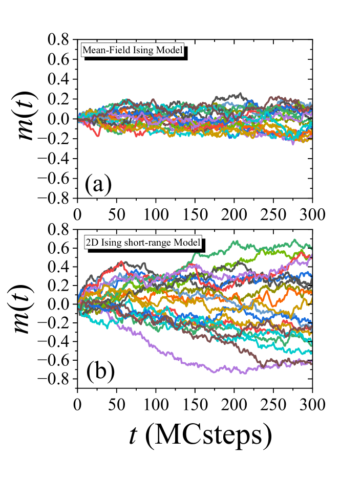
Figure 1: A sample of magnetization time evolutions to be used for obtaining the matrices and thus, performing the spectral study. Plot (a) shows the series of mean-field Ising model that is the subject of this current study. Plot (b) shows (for comparison) the results for the two-dimensional Ising model. Both systems are simulated in their respective critical temperatures

A sample of magnetization time evolutions to be used for obtaining the matrices and thus, performing the spectral study. Plot (a) shows the series of mean-field Ising model that is the subject of this current study. Plot (b) shows (for comparison) the results of the two-dimensional Ising model. We observe that the mean-field series seems to be present less variability than the time series of the two-dimensional short-range Ising model. But the question persists: should matrices $G$ built from MF Ising data produce spectra that can describe the thermodynamics of this model?

Thus we build our ensemble of matrices, considering $N_{run}=1000$ different matrices $G$ ($N_{sample}\times N_{sample}$). Then, we diagonalize them and categorize the data between $\lambda_{\min}^{(\text{Numerical})}$ and $\lambda_{\max}^{(\text{Numerical})}$ among all eigenvalues, keeping the number of bins fixed in $N_{bin}=100$.

We repeated the process for several different temperatures between $T_{\min}=\frac{1}{2}T_{C}$ until $T_{\max}=\frac{13}{2}T_{C}$, recalling that $T_{C}=Jz/k_{B}$ (which is exactly 1 in our reduced units). We show the numerical density of eigenvalues for the different temperatures in (Fig. 2).

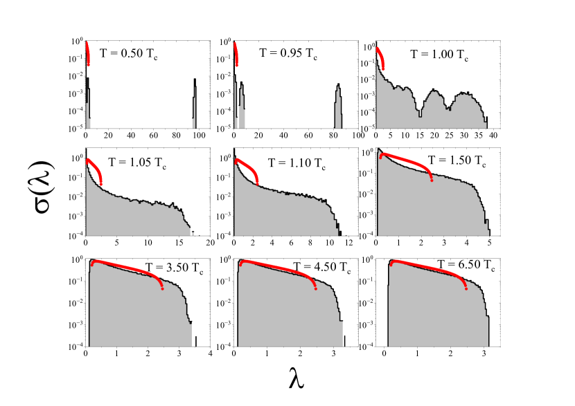
Figure 2: Density of eigenvalues for different temperatures. We observe that for $T=T_{C}$, there is no gap between two groups of eigenvalues that occurs for $T<T_{C}$. For $T>T_{C}$ the density approaches to Marchenko-Pastur law (Eq. 9) indicates that magnetization time series become uncorrelated. The red continuous curve corresponds to Marchenko-Pastur density for comparison.

We observe that for exactly $T=T_{C}$, there is no gap between two groups of eigenvalues that occurs for $T<T_{C}$. For $T>T_{C}$, the density approaches to Marchenko-Pastur law (Eq. 9), indicating that magnetization time-series become uncorrelated.

Now, the first step of our study is ready. The spectra responded to the the temperature of the system and apparently the gap between the eigenvalues reduces to a single bulk. This also occurs with two-dimensional Ising and Potts model (see RMT2023 ; RMT2023-2 ). It is worth emphasizing that in a direct comparison between these short-range systems with the current MF one, the gap closing occurs exactly at $T=T_{C}$ while for the former, we need to have a temperature a little higher than $T_{C}$ ($T\approx 1.10T_{C}$).

However, independently of that, when we look at eigenvalues fluctuations, our method is precise in asserting where is the critical temperature as shown in Fig. 3. The results were obtained via MC simulations from Glauber and Metropolis dynamics and they show very good agreement.

Figure 3: Average eigenvalue and variance of the eigenvalue as a function of $T/T_{C}$. We observe a minimum on the average eigenvalue at $T=T_{C}$, concurrently with an inflection of the variance at the same temperature.

By estimating the numerical moments:

$$\left\langle\lambda^{k}\right\rangle=\frac{\sum\limits_{i=1}^{N_{bins}}\lambda_{i}^{k}\sigma^{(\text{Numerical)}}(\lambda_{i})}{\sum\limits_{i=1}^{N_{bins}}\sigma^{(\text{Numerical)}}(\lambda_{i})}\text{,}$$

we observe in the Fig. 3, the average eigenvalue as as function of $T/T_{C}$, as well as the dispersion $\left\langle(\Delta\lambda)^{2}\right\rangle=\left\langle\lambda^{2}\right\rangle-\left\langle\lambda\right\rangle^{2}$ as function of the same quantity. We performed MC simulations in this case for both Glauber and Metropolis dynamics. We observe a minimal of the average eigenvalue at $T=T_{C}$, concurrently with an inflection of the variance at the same point.

Thus we can conclude that for this MF regime, the spectra of eigenvalues of Wishart matrices built from magnetization time series work exactly as the short-range models. However, it is interesting to investigate what occurs directly on the correlations between the time series. Thus we build histograms of elements of matrices $G$ directly in different temperatures which can observe in Fig 4.

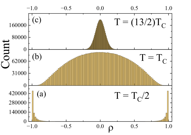
Figure 4: Histograms of the correlations between different time evolutions for the Mean-field Ising. Such study was performed for three different temperatures, starting from random initial configurations. (a) $T=T_{C}/2$, (b) $T=T_{C}$, and (c) $T=6T_{C}/5$, showing strong correlation, indetermination, and decorrelation respectively, exactly as occurs in short-range systems studied with the same method.

Magnetization has a growth trend over the different evolutions when the system suddenly quenches to a temperature $T=\frac{1}{2}T_{C}$. This the tendency of ordering generates correlations between the different evolutions corroborated by Fig. 4 (a), where considerable negative or positive correlations occur depending on the initial configuration.

However, when the system quenches to a temperature $T=T_{C}$ (Fig. 4 (b)), we see that correlation distribution is broadly distributed. This is an intermediate situation that characterizes the spontaneous breaking of symmetry.

The system becomes uncorrelated (no novelty) when the relaxation occurs from a high temperature $T=\frac{13}{2}T_{C}$ (Fig. 4 (c)). Such qualitative behavior reflects on the spectra of Wishart matrices, whose fluctuations can determine with precision the critical point of the system

4 Conclusions and summaries

Our purpose here was to apply a method of studying the spectra of eigenvalues of Wishart matrices of magnetization time series for a long-range spin system: the mean-field Ising model. Exactly as applied in previous contributions (see refs. RMT2023 ; RMT2023-2 ) in short-range systems, we showed here that the method can also be applied to a mean-field system with time series obtained from Monte Carlo simulations.

We believe that the method is promising and that it should be tested in strict long-range systems, other magnetic spin systems, and nonequilibrium models, among others.

It will be interesting to study the use of Wishart matrices in unsupervised learning as those proposed, for example, in Refs. wang2016 ; tirelli2022 .

Compliance with Ethical Standards

Funding: R. da Silva thanks CNPq for financial support under the grant numbers 311236/2018-9 and 304575/2022-4.

Conflict of Interest: The authors declare that they have no known competing financial interests or personal relationships that could have appeared to influence the work reported in this paper.

Ethical Conduct: The authors declare that they did not violate any ethical conduct in preparing this paper.

References

- (1) S. R. A. Salinas Introduction to Statistical Physics, Springer (2001)
- (2) W. F. Wreszinski, S. R. A. Salinas, Disorder and Competition in Soluble Lattice Models. World Scientific, (1993)
- (3) J. R. Drugowich de Felício, V. Líbero, Am. J. Phys. 64, 1281 (1996)
- (4) E. F. Henriques, V. B. Henriques, S. R. Salinas, Phys. Rev. B 51, 8621 (1995)
- (5) T. Tome and M. J. Oliveira, Stochastic Dynamics and Irreversibility, Springer, Cham (2015)
- (6) C. Anteneodo, E. E. Ferrero, S. A. Cannas, J. Stat. Mech., P07026 (2010)
- (7) R. da Silva, Braz. J. Phys. 52, 128 (2022)
- (8) B. Zheng, Int. J. Mod. Phys. B 12, 1419 (1998)
- (9) T. Tome, M. J. de Oliveira, Phys. Rev. E 58, 4242 (1998)
- (10) T. Tome, Braz. J. Phys. 30, 152 (2000)
- (11) D. A. Huse. Phys. Rev. B 40, 304 (1989)
- (12) H. K. Janssen, B. Schaub, B. Schmittmann, Z. Phys. B: Condens. Matter 73, 539 (1989)
- (13) R. da Silva, H. A. Fernandes, J. R. Drugowich de Felicio Phys. Rev. E 90 042101 (2014)
- (14) R. da Silva. H. A. Fernandes, J. Stat. Mech., P06011 (2015)
- (15) R. da Silva, M. J. de Oliveira, T. Tome, and J. R. Drugowich de Felicio, Phys. Rev. E 101, 012130 (2020)
- (16) H. Hinrichsen Adv. Phys. 49, 815-958 (2000)
- (17) J. Marro, R. Dickman, Nonequilibrium Phase Transitions in Lattice Models, Cambridge (1999)
- (18) M. Henkel, M. Pleimling, Non-equilibrium Phase Transitions, Vol. 2: Ageing and Dynamical Scaling far from Equilibrium, Springer, Dordrecht (2010)
- (19) R. da Silva, J. R. Drugowich de Felicio, and A. S. Martinez, Phys. Rev. E 85, 066707 (2012)
- (20) R. da Silva, Int. J. Mod. Phys. C, 2350061 1 (2023)
- (21) R.da Silva, E. Venites, S. D. Prado, J. R. Drugowich de Felício, ArXiv. https://doi.org/10.48550/arXiv.2302.07990 (2023)
- (22) E. P. Wigner, Ann. Math. 53, 36 (1951)
- (23) E. P. Wigner, Ann. Math. 62, 548 (1955)
- (24) M. L. Mehta, Random Matrices, Academic Press, Boston (1991)
- (25) Y. Sinai, A. Soshnikov, Bol. Soc. Bras. Mat. 29, 1 (1998)
- (26) F.J. Dyson, J. Math. Phys. 3, 140–156, 157–165, 166–175 (1962)
- (27) J. Wishart, Biometrika 20A, 32 (1928)
- (28) T. Guhr, A. Muller-Groeling, H. A. Weidenmuller, Phys. Rep. 299, 189 (1998)
- (29) Vinayak, T. H. Seligman, AIP Conf. Proc. 1575, 196 (2014)
- (30) V. A. Marcenko, L. A. Pastur, Math. USSR Sb. 1 457 (1967)
- (31) L. Wang, Phys. Rev. B 94, 195105 (2016)
- (32) A. Tirelli, D. O. Carvalho, L. A. Oliveira, N. C. Costa, R. R. dos Santos, The European Physical Journal B 95 189 (2022)