Discovery and Recognition of Formula Concepts using Machine Learning

Abstract

Citation-based Information Retrieval (IR) methods for scientific documents have proven effective for IR applications, such as Plagiarism Detection or Literature Recommender Systems in academic disciplines that use many references. In science, technology, engineering, and mathematics, researchers often employ mathematical concepts through formula notation to refer to prior knowledge. Our long-term goal is to generalize citation-based IR methods and apply this generalized method to both classical references and mathematical concepts. In this paper, we suggest how mathematical formulas could be cited and define a Formula Concept Retrieval task with two subtasks: Formula Concept Discovery (FCD) and Formula Concept Recognition (FCR). While FCD aims at the definition and exploration of a ‘Formula Concept’ that names bundled equivalent representations of a formula, FCR is designed to match a given formula to a prior assigned unique mathematical concept identifier. We present machine learning-based approaches to address the FCD and FCR tasks. We then evaluate these approaches on a standardized test collection (NTCIR arXiv dataset). Our FCD approach yields a precision of 68% for retrieving equivalent representations of frequent formulas and a recall of 72% for extracting the formula name from the surrounding text. FCD and FCR enable the citation of formulas within mathematical documents and facilitate semantic search and question answering as well as document similarity assessments for plagiarism detection or recommender systems.

Keywords Mathematical Information Retrieval  $\cdot$ Search  $\cdot$ Machine Learning  $\cdot$ Classification  $\cdot$ Clustering  $\cdot$ Wikidata

1 Introduction

Documents from Science, Technology, Engineering, and Mathematics (STEM) often contain a significant amount of mathematical formulas Hambasan and Kohlhase (2015). Formulas are a vital non-textual component to understand the content of STEM documents. Systems, such as semantic search engines, question answering systems, and document recommender systems, should also be capable of processing formulas and their connections with the surrounding text and mathematical expressions. In information science and technology, the semantics of natural language is typically grasped via conceptualization Yucong and Cruz (2011). According to Gruber (1993), the term conceptualization refers to the process of simplifying the representation of objects of discourse and specifying a semantic vocabulary in an ontology (knowledge system). Analogously, to capture the semantics of mathematical language in formulas, we argue for the introduction of a mathematical Formula Concept, which we define as a collection of equivalent formulas with different representations (see also Section 3 below). This extends the definition of the formula content comprising constituents, relations, and semantics of a formula, which was introduced in  Scharpf et al. (2018). We select the Klein–Gordon equation as an example for mathematical conceptualization. Figure 1 shows different representations of the Klein–Gordon equation from quantum mechanics (also referred to as a relativistic wave equation). These representations of the Klein–Gordon equation in the academic literature appear to be diverse, but they all represent the same mathematical concept. Employing additional mathematical Formula Concept examples, we illustrate and discuss differences and explain the resulting challenges of this conceptualization process in detail. We introduce two tasks: Formula Concept Discovery (FCD) and Formula Concept Recognition (FCR) to (1) identify Formula Concepts and (2) find formulas which are instances of particular Formula Concepts.

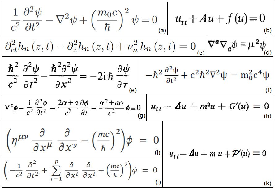
Figure 1: Representations of the Klein–Gordon equation extracted from physics papers - (a): Arbab (2010), (b): Pecher (1984), (c): Tretyakov and Akgun (2010), (d): Detweiler (1980), (e): Kaloyerou and Vigier (1989), (f): Haroun et al. (2017), (g): Tiwari (1988), (h): Strauss and Vazquez (1978), (i): nLab authors , (j): nLab authors , (k): Morawetz (1968). Some of the representations are written in a general, potentially nonlinear form. With constraints given for the parameters in the respective publications, the equations become the linear Klein–Gordon equation.

We present implementations to automatically perform the FCD and FCR tasks using machine learning techniques.

Novelty of Contribution.

This paper extends our previous publication Scharpf et al. (2019a), in which we introduced the first FCD retrieval method implementation. We extend our study of Formula Concepts by two additional FCD retrieval methods, three additional tasks, and the entire section on FCR experiments. A strong focus of this work is placed on the in-depth analytical examination of example Formula Concepts. We discuss 36 different representations of the Klein–Gordon equation, Einstein’s field equations, and Maxwell’s equations. Analyzing their differences, we identify 13 challenges for FCD to derive requirements for the practical implementation of an FCD framework. Furthermore, we investigate the Formula Concept vector space of our examples in four different formula encodings (vector representations). Additionally, we examine the separability or delineation of different Formula Concepts by computing classification accuracy (SVM classifier) and cluster purity ($k$-means clusterer). We also generate formula similarity maps in different encoding measures to illustrate FC class coherence. Finally, we present and discuss several of our FCR implementations, including search rankings and additional machine learning methods.

2 Related Work

This section reviews and explains some background knowledge necessary to understand this research project. This includes our own preliminary work and achievements to tackle FCD, related methods of Mathematical Entity Linking, formula knowledge bases, STEM document dataset sources, and mathematical information system applications.

We recently introduced a first machine learning approach for Formula Concept Discovery Scharpf et al. (2019b). Using Doc2Vec Le and Mikolov (2014) encodings and $k$-means clustering, equivalent representations of formulas were retrieved and evaluated. The experiment was carried out on a selection of astrophysics papers from the NTCIR arXiv dataset Aizawa et al. (2014). We took formulas that occurred most often in the corpus (duplicates) as a cluster seed. Furthermore, for the major part of the test selection candidates, a valid Formula Concept name could be retrieved from the surrounding text. For almost all of the retrieved name candidates, a Wikidata QID was available.

In this paper, we extend our Formula Concept Discovery method by novel Formula Concept Recognition methods. Both approaches involve two steps: knowledge-base population and content referencing. These can both be described in terms of Mathematical Entity Linking (MathEL) Scharpf et al. (2021a, b). MathEL approaches link mathematical formulas to unique URLs in a semantic knowledge base. If the URLs are part of Wiki web resources, MathEL can be regarded as the ‘Wikification’ of mathematical content Kristianto et al. (2016).

In Natural Language Processing, Entity Linking entities are typically linked to Wikipedia with a variety of applications, such as Named Entity Recognition (NER), relationship extraction, entity summarization Rosales-Méndez et al. (2018). In analogy, methods to link mathematical expressions in scientific documents to Wikipedia articles using their surrounding text have been developed Kristianto et al. (2016); Kristianto and Aizawa (2017). One of the conclusions was that for the linking to be reliable, a balanced combination of textual and mathematical elements must be considered. As potential candidates for MathEL, Mathematical Objects of Interest (MOI) were defined to elaborate methods for their discovery Greiner-Petter et al. (2020). MathEL is expected to enhance mathematical subject classification Scharpf et al. (2020a); Schubotz et al. (2020).

To implement our FCR methods, we employ Wikidata as the semantic grounding for Wikification (entity linking to Wiki web resources). Since Wikipedia is only semi-structured, Wikidata was launched to provide direct access to specific interlingual facts (RDF triples) and to retrieve information systematically.
Wikidata is a free and open semantic knowledge base that can be read and edited by humans and machines Vrandecic and Krötzsch (2014). Wikidata stores items with statements and references. In the case of mathematical knowledge, this may include formulas. For example, one may describe the physics concept ‘pressure’ (item ID Q39552) with a ‘defining formula’ property (property ID P2534) $p=F/S$. To scalably seed information into Wikidata, a primary sources tool (PST) was introduced. This tool allows active users to quickly browse through new claims and references in order to approve or reject their validity. Currently, Wikidata contains approximately 5,7K items with a ‘defining formula’ property.

Besides Wikidata, other semantic databases exist that store mathematical formula knowledge. The NIST Digital Library of Mathematical Functions DLMF and NIST Digital Repository of Mathematical Formulae (DRMF) Cohl et al. (2014) are two examples of maintained high-quality semantic datasets. Moreover, the benchmark MathMLben Schubotz et al. (2018a) was created to evaluate tools for mathematical format conversion (from LaTeX to MathML to Computer Algebra Systems), containing almost 400 formulas from Wikipedia, the arXiv, and DLMF. These were augmented by Wikidata macros in Scharpf et al. (2018).

Mathematical Information Retrieval (MathIR) systems address the information need of people working in STEM fields by retrieving, processing, and analyzing mathematical formulas Scharpf et al. (2018). Up until now, various formula search engines have been developed. Furthermore, translations between different markups (LaTeX, Presentation, and Content MathML) and standards have been introduced Guidi and Coen (2016). Schubotz et al. present a framework to translate MathML into Computer Algebra System (CAS) syntax. Furthermore, standards like OpenMath and OMCDoc provide extensible ways to represent the semantics of mathematical objects in mathematical documents Kohlhase (2006). They can be used to annotate formula expressions in definitions, theorems, and proofs. Given markup on object, statement, and theory level, the soundness of mathematical systems can be assessed Scharpf et al. (2018). In addition, the PhysML variant accounts for the special characteristics of physics: observables, physical systems, and experiments Hilf et al. (2006). Moreover, Mathematical Question Answering (MathQA) systems have been built Schubotz et al. (2019); Scharpf et al. (2022a) to provide quick and concise formula answers to mathematical questions in natural language which are commonly asked on the web Scharpf et al. (2020b). MathQA systems can retrieve answers from unstructured text passages or structured knowledge bases. In the latter case, MathEL needs to be employed to assign natural language concept names to mathematical formulas. While classical math search engines typically map a mathematical language query (formula string) to a collection of web resources that include the natural language name of the Formula Concept Kohlhase and Sucan (2006), MathQA systems perform the reverse transformation from natural to mathematical language. Another application of the mapping from mathematical to natural language using MathEL is question generation Scharpf et al. (2022b).

For some Mathematical Language Processing (MLP) applications, the formula constituents (operators, identifiers, numbers) have to be annotated using Mathematical Markup Language (MathML). There are several tools available to convert LaTeX into MathML, most prominently the LaTeXML converter. Furthermore, the occurring symbols (variables, constants) need to be disambiguated, i.e., their meaning inferred from the context by unsupervised retrieval or supervised annotation. There have been previous attempts to automatically retrieve the semantics of identifiers from the surrounding text Schubotz et al. (2016); Greiner-Petter et al. (2022). However, it was found that not all identifier names could be extracted from the text. To address this, Schubotz et al. cluster identifier namespaces to enable a fallback retrieval from the definition cluster. While Wikipedia articles commonly contain variable definitions in the text, many paper articles often omit them, assuming expert reader domain knowledge. To build machine-interpretable datasets, manual annotation is thus inevitable. Since this is very time-consuming, formula and identifier annotation recommender systems, such as ‘AnnoMathTeX’ Scharpf et al. (2019b, 2021a) are built to speed up the process.

To create labeled formula data benchmarks, we need open access corpora of STEM documents. For research experiment reproducibility, snapshots must be defined. The arXiv.org e-Print archive McKiernan (2000) makes available free preprints for an extensive collection of publications from physics, mathematics, computer science, economics, and other fields. On the arXiv, many authors provide their LaTeX source code. Both Wikipedia and arXiv articles were extracted as part of the NTCIR MathIR Task Aizawa et al. (2014). We employ the NTCIR arXiv dataset for our research in this paper. In 2017, the Special Interest Group for Math Linguistics (SIGMathLing) was initiated as a forum and resource cooperative for the linguistics of mathematical or technical documents.

3 Formula Concept Discovery

In this section, we attempt to formally define a Formula Concept and set up Formula Concept Retrieval Tasks.

3.1 Formula Concept Retrieval Tasks

Definition.

Following Scharpf et al. (2018), we define the formula content as the sets of operators, identifiers, and numbers that a formula contains. Furthermore, we define a Formula Concept as a collection of equivalent formulas with different representations featuring the same formula content (operators, identifiers, and numbers). Consider the Klein–Gordon equation representations in Figure 1 as an example of a Formula Concept. Obviously, the formula content may vary as the occurring operators, identifiers, and numbers change from instance to instance. Operators such as partial derivatives can be represented in several ways ($\partial^{2}u/\partial t^{2}$ vs. $u_{tt}$ vs. $\ddot{u}$), identifiers can be subsumed into others (e.g., $\alpha=mc/\hbar$), and physical constants can be transformed to different unit systems (e.g., natural units with $\hbar=c=1$). The Formula Concept Discovery challenges will be discussed in more detail in Section 3.4. This motivates our study to find out what equivalent representations can occur and how to handle them.

Tasks.

Our goal is to map diverse representations of a formula to one unique Formula Concept ID, e.g., linking all occurrences of the Klein–Gordon equation shown in Figure 1 to the Wikidata item Q868967. We define two subtasks of the Formula Concept Retrieval Task:

• Formula Concept Discovery is a method to find common equivalent representations and a name candidate for a given formula, and

• Formula Concept Recognition is an approach for recognizing formulas in documents as being instances of a previously defined Formula Concept.

In the following, we present our implementation and evaluation results for Formula Concept Discovery and Formula Concept Recognition. These results are based on analytical examinations, machine learning, fuzzy string matching, and Wikipedia article heuristics.

For the discovery of Formula Concepts, we define the following four tasks:

1. [Task 1:]

2. Retrieval of Formula Concept examples,

3. Analysis of Formula Concept examples,

4. Identification of Formula Concept Discovery challenges,

5. Derivation of Formula Concept Retrieval system requirements.

In Task 1, we employ three methods to retrieve examples of Formula Concepts, which are suitable for discussing and identifying challenges of Formula Concept Discovery and Formula Concept Recognition. In Task 2, we analyze and discuss three selected Formula Concept examples. We choose three sets of differential equations from physics: the Klein–Gordon equation (KGE), Einstein’s field equations (EFE), and Maxwell’s equations (ME). The examples are retrieved from search engine results for the Formula Concept name yielding publications (sources as in Figure 1), as well as from Wikipedia article content15, and a textbook Fließbach (1990). Given our background in theoretical physics and applied mathematics, we choose examples from this domain. Since we are domain experts on the topics, we can judge the Formula Concept semantics. The formula annotation is achieved in a two-step process: 1) the retrieval by the concept name in the selected sources determines the annotation or assignment of the whole formula; 2) the domain expert subsequently semantically analyzes the formula and retrieves the semantic annotations of the formula constituents by considering the context and descriptions or explanations from the respective sources (text surrounding the formula). In Task 3, we identify and summarize the Formula Concept Discovery challenges, which we observe in the discussion of the three Formula Concept examples. These challenges determine the requirements for technical implementations of FCD and FCR. In Task 4, we address the identified challenges by deriving requirements for a Formula Concept Retrieval system and proposing methods to tackle the challenges.

The developed algorithms, the dataset, and full result tables are available at https://github.com/ag-gipp/formula-concept-retrieval.

3.2 Task 1: Retrieval of Formula Concept Examples

For the retrieval of example Formula Concepts, we employ the following three methods:

1. [Method 1:]

2. Search by Formula Concept Name,

3. $k$-Nearest-Neighbors ($k$NN) in Formula Vector Space,

4. Wikipedia article First Formula Multi-Language Heuristic.

In Method 1, we perform searches by the Formula Concept name in a corpus of publications, a Wikipedia article, and a textbook, respectively. In Method 2, we employ machine learning to retrieve equivalent representations of formulas Scharpf et al. (2019b), which occur most often (duplicates) in a selected corpus containing astrophysics papers from the NTCIR arXiv dataset Aizawa et al. (2014). For an introduction of the dataset, see the paragraph ‘Data selection’ in Section 3.2.2. In Method 3, we make use of a simple heuristic Schubotz et al. (2018b); Halbach (2020). We take the tentative Formula Concept names of the examples retrieved using Method 2. We then extract the corresponding Wikipedia articles. For each Formula Concept article, we retrieve the first five versions in different languages. We then assess how many different representations of the individual Formula Concepts are among these articles.

3.2.1 Method 1: Search by Formula Concept Name

For our first example, the Klein–Gordon equation, we perform a web search to retrieve ten representations from publications Arbab (2010); Detweiler (1980); Haroun et al. (2017); Kaloyerou and Vigier (1989); Morawetz (1968); Pecher (1984); Strauss and Vazquez (1978); Tiwari (1988); Tretyakov and Akgun (2010). Each publication contains the Formula Concept name as a keyword or in the full text. For our second example, Einstein’s field equations, we retrieve representations from the corresponding Wikipedia article. For our third example, Maxwell’s field equations, we take derivations from a textbook on General Relativity Fließbach (1990).

3.2.2 Method 2: $k$-Nearest-Neighbors in Formula Vector Space

This subsection is based on our previous publication Scharpf et al. (2019b), in which we presented Formula Concept Discovery using $k$-Nearest-Neighbors for the first time. Since it might be impossible to formally define all equivalence transformations exhaustively, we test approaching a Formula Concept in machine learning terms as a collection of approved formula vectors (comparing encodings) within a specified similarity range (comparing metrics). We illustrate the formula space (formula content space in Figure 4 and formula semantic space in Figure 5) in Experiment 2 of FCR in Section 4.2. It represents formulas as encoded vectors. Then, a Formula Concept can be defined as all vectors around a central vector within a specified distance (cutoff).

Method.

We approach the discovery of Formula Concepts by retrieving equivalent formulations with different representations using machine learning (see Figure 2). The retrieved instances are augmented with name candidates from the surrounding text. The initial step is to identify formula candidates that occur most often within a given dataset. We assume that they are potential seeds of popular Formula Concepts. We first tried formula clustering Adeel et al. (2012); Ma et al. (2010). However, we discovered that this was not a suitable method for FCD since the number of clusters is a priory unclear. The tested algorithms are not able to group equivalent formulas. Subsequently, we decided to start with a ranking of formula duplicates (with the same LaTeX string). In contrast to the clustering, this yields valuable results for the selected Formula Concept examples.

Hubble’s law (Q179916)	Equation of state (Q214967)
$\!\begin{aligned} p&=\omega\rho\\ p&=\kappa\rho\\ \omega&=p/\rho\\ p_{d}&=\omega\rho_{d}\\ \end{aligned}$	$\!\begin{aligned} \dot{a}&=aH\\ H_{i}&=\dot{R}/R\\ H&=\dot{a}/a\\ H(t)&=\dot{a}/a\\ \end{aligned}$

Figure 2: Clustering equivalent representations of formulas in the semantic space as named Formula Concept Wikidata items.

Data Selection.

We employ the NTCIR arXiv dataset Aizawa et al. (2014), which comprises 105,120 document sections containing over 60 million formulas. The formulas are enclosed in <math> tag environments. The documents were converted from LaTeX to an XHTML format (https://tei-c.org). The disk size of the dataset is about 174GB uncompressed. We confine our computations to the subject class of astrophysics (680 astro-ph documents), employing a domain expert to evaluate the results semantically. To get the most popular formulas in the dataset as potential candidates for important Formula Concepts, we first identify duplicates where the exact formula string reoccurs in multiple documents. We subsequently rank the results by their occurrence frequency, i.e., the number of duplicates $d$ (see the respective column in Table 1). From the duplicate ranking, we select a formula length range between 10 and 30 characters and restrict our selection to duplicates occurring in at least two documents $D\geq 2$. This selection criteria processing results in 3,495 formulas. We then manually select all equations (for now, we confine the Formula Concept definition to include equations only). We discard all stubs without a right-hand side, as well as simple variable dependence definitions, such as $x=x\left(t\right)$ and $x=y$ or $x=\mathrm{const}$. The algorithms for the data selection pipeline can be found in the source repository.

Evaluation.

For the first 50 samples from the duplicate ranking, we retrieve the operators and identifiers from the provided MathML <mo> and <mi> tags, as well as the surrounding text (words within a window of $\pm 500$ characters around the formula). We encode both tag contents using the TfidfVectorizer from the Python package Scikit-learn Pedregosa et al. (2011) and Doc2Vec model Le and Mikolov (2014) from the Python package Gensim Rehurek (2011). We then assess the performance of a $k$-Nearest-Neighbors classifier Shakhnarovish et al. (2005) to retrieve equivalent formula representations. For a given instance of a Formula Concept, we compute the $k$-Nearest-Neighbors formulas as candidates for variations of that Formula Concept. Subsequently, we use our domain knowledge to judge whether these candidates are indeed equivalent representations of the given Formula Concept. We test the effectiveness of our approach on four different formula vector encodings:

• math2vec encoding the formula constituents using the Doc2Vec model as proposed in Youssef and Miller (2018);

• math tf-idf encoding the formula constituents using the TfidfVectorizer;

• semantics2vec encoding the surrounding text (containing tentative formula semantics) using the Doc2Vec model; and

• semantics tf-idf encoding the surrounding text using the TfidfVectorizer.

The computation of the Doc2Vec formula vector encodings is more time-expensive than TF-IDF, due to the iterative learning process of the neural model.

Results.

Table 1 shows the results of our approach for discovering Formula Concepts as published before Scharpf et al. (2019a). We rank the extracted formulas by the number of duplicates $d$ and list the number of documents $D$, in which they appear. Note that the likelihood of retrieving non-duplicate equivalent representations increases for higher values of distinct documents. If the Formula Concept representations are found in different documents, there are more than if they appear in the same document. This means that there are fewer variations within the same document. We can see that only for the first 18 Formula Concept examples are there more than two duplicates from distinct documents, i.e., formulas appearing twice or more within the corpus. We evaluate the first 50 examples. The primary investigation was to compare the performance of four different formula vector encodings in terms of the retrieved number of equivalent representations. In total, we can retrieve 163 equivalent Formula Concept representations for our 50 samples. On average, this corresponds to more than three (163/50 = 3.3) per formula (from 3 different documents) or around one (163/50/4 = 0.8) per source per formula. Some of the retrieved formulas even contain different identifier symbols or varying indices (e.g., a is replaced by R in Example 1, see the first line of Table 1). Increasing the number of formula neighbors parameter $k$ from 1 in integer steps, we can not find additional matching representations above $k=9$. We define the retrieval success $s$ of an individual encoding as the percentage of retrieved representations compared to all other formula vector encodings. Calculating the overall success distribution, we discover that the math2vec ($e_{m}$) encoding distinctively outperforms the others by yielding 71% of the retrieved instances, followed by semantics tf-idf, ($\hat{e}_{s}$) with 15%, semantics2vec ($e_{s}$) with 11%, and math tf-idf ($\hat{e}_{m}$) with 4%. Overall, for 34 of the investigated 50 sample formulas, i.e., 34/50 = 68%, we are able to retrieve equivalent representations. We conclude that while the math2vec encoding retrieves the most equivalent formula matches as candidates for a Formula Concept, it is most effective to employ all formula vector encodings simultaneously to maximize the retrieval. Note that we can only determine false positives and compute precision but not the number of false negatives to compute recall. This is because we do not know a priori how many different equivalent representations, semantically close to the examined concept, still exist. We can neither determine this in general (how many notational variations are possible in principle) nor for the given corpus (how many do occur). Finally, we list the top five name candidates from the surrounding text. The word window size is chosen to be $\pm$500 characters. Decreasing the window size in steps of 100, the top 50 coverage performance drops from 100% to 17% to 11% for $\text{ws}=\{500,400,300\}$ to $\text{ws}=200$ to $\text{ws}=100$ respectively. We evaluate whether they contain a suitable name for the Formula Concept to be seeded as a Wikidata item. For our 50 Formula Concept examples, we achieve a recall of 36/50 = 72% for the formula name. Furthermore, for 41/50 = 82% of the retrieved name candidates, a Wikidata QID is available to tag the Formula Concept.

Table 1: Formula Concept Discovery Scharpf et al. (2019a). Top-50 results of a cross-document duplicate search in the subject class astro-ph of the NTCIR arXiv dataset. Equivalent formulas are retrieved to bundle mathematical concept candidates using a $k$-Nearest-Neighbors ($k$NN) recommendation, while comparing the relative success $s$ of different formula vector encodings (math2vec: $e_{m}$, math tf-idf: $\hat{e}_{m}$, semantics2vec: $e_{s}$, semantics tf-idf: $\hat{e}_{s}$). The number of duplicates $d$ and originating distinct documents $D$ are shown as well as a retrieved sample formula. Furthermore, it is evaluated whether the first five words of the surrounding text are candidates for the formula’s name, and whether a Wikidata QID is available.

Nr.	Formula	Name (QID)	$d$ / $D$	$s_{{e_{m}}},s_{{\hat{e}_{m}}},s_{{e_{s}}},s_{{\hat{e}_{s}}}$	Encoding: sample
1	$H=\dot{a}/a$	Hubble parameter (Q179916)	32 / 32	$0$, $0.1$, $0$, $0.9$	${\hat{e}_{s}}$: $H_{i}=\dot{R}/R$
2	$p=\omega\rho$	Equation of state (Q214967)	6 / 5	$0.29$, $0$, $0.14$, $0.57$	${e_{s}}$: $p_{d}=w\rho_{d}$
3	$\omega=p/\rho$	Accelerating universe (Q1049613)	4 / 3	$0.67$, $0$, $0$, $0.33$	${e_{m}}$: $p=\omega\rho$
4	$p=-A/\rho^{\alpha}$	Dark fluid (Q5223514)	4 / 4	$0.67$, $0$, $0.33$, $0$	${e_{m}}$: $p=-\frac{A}{\rho^{\alpha}}$
5	$p_{d}=w\rho_{d}$	Dark energy (Q18343)	4 / 3	$0.33$, $0$, $0.33$, $0.33$	${e_{s}}$: $p_{X}=\omega_{X}\rho_{X}$
6	$H={\dot{a}}/a$	Hubble’s law (Q179916)	4 / 4	$0.4$, $0.1$, $0.2$, $0.3$	${\hat{e}_{m}}$: ${\mathcal{H}}=a^{\prime}/a$
7	$k=|{\bf k}|$	Wavenumber (Q192510)	3 / 3	$0.83$, $0$, $0.17$, $0$	${e_{m}}$: $k=|\vec{k}|$
8	$f=e^{-\phi}R$	N/A	3 / 2	$1$, $0$, $0$, $0$	${e_{m}}$: $f(\phi)=e^{-\phi}R$
9	$p=\kappa\rho$	Equation of state (Q214967)	3 / 2	$0.33$, $0$, $0.67$, $0$	${e_{s}}$: $p_{D}=w(z)\rho_{D}$
10	$w=p_{X}/\rho_{X}$	Equation of state (Q214967)	3 / 3	$0.62$, $0$, $0.12$, $0.25$	${e_{m}}$: $p_{X}=w_{X}\rho_{X}$
11	$\mu=m_{p}/m_{e}$	Proton-to-electron mass ratio (Q2912520)	3 / 3	$1$, $0$, $0$, $0$	${e_{m}}$: $m_{i}=\mu m_{p}$
12	$\phi_{c}=M/g$	Critical value (Q2189464)	3 / 3	$0$, $0$, $0$, $0$	N/A
13	$p=-\frac{A}{\rho^{\alpha}}$	Chaplygin gas (Q5073250)	3 / 3	$0.8$, $0$, $0$, $0.2$	${e_{m}}$: $p=-A\rho^{-\alpha}$
14	$p=\alpha\rho$	Polytropic gas (Q831024)	3 / 2	$0.67$, $0$, $0.17$, $0.17$	${\hat{e}_{s}}$: $w_{\alpha}=p_{\alpha}/\rho_{\alpha}$
15	$M=\widetilde{M}/\Gamma$	Connected manifold (Q2721559)	3 / 3	$0$, $0$, $0$, $0$	N/A
16	$g(a)=\bigtriangleup(a)/a$	Dark energy (Q18343)	3 / 2	$1$, $0$, $0$, $0$	${e_{m}}$: $g(a)=\Delta(a)/a$
17	$\alpha=dn_{s}/d\ln{k}$	Wavenumber (Q192510)	3 / 3	$1$, $0$, $0$, $0$	${e_{m}}$: $dn_{s}/d\ln k=\alpha_{s}$
18	$\psi=-i\theta$	N/A	3 / 2	$0$, $0$, $0$, $0$	N/A
19	$dt=a(\eta)d\eta$	Time (Q11471)	2 / 2	$0.5$, $0$, $0.25$, $0.25$	${\hat{e}_{s}}$: $t=\int a(\eta)d\eta$
20	$\Delta x_{min}=\sqrt{\beta}$	Lower bound (Q21067468)	2 / 2	$1$, $0$, $0$, $0$	${e_{m}}$: $\Delta x_{\rm min}=\hbar\sqrt{\beta}$
21	$k^{i}=ap^{i}$	Modes (N/A)	2 / 2	$0$, $0$, $0$, $0$	N/A
22	$\varphi=\delta A_{\mu}$	Perturbations (Q911364)	2 / 2	$0$, $0$, $0$, $0$	N/A
23	$h_{ab}=g_{ab}-n_{a}n_{b}$	Metric (Q865746)	2 / 2	$0$, $0$, $0$, $0$	N/A
24	$K=K_{ab}h^{ab}$	Brane (Q385601)	2 / 2	$1$, $0$, $0$, $0$	${e_{m}}$: $K=K_{\alpha\beta}h^{\alpha\beta}$
25	$v=\sqrt{|dp/d\rho|}$	Equation of state (Q214967)	2 / 2	$1$, $0$, $0$, $0$	${e_{m}}$: $v_{c}=\sqrt{dp_{c}/d\rho_{c}}$
26	$Q=\sqrt{G}M$	Limit (Q246639)	2 / 2	$0$, $0$, $0$, $0$	N/A
27	$\zeta=H\delta\phi/\dot{\phi}$	Perturbation theory (Q10886678)	2 / 2	$1$, $0$, $0$, $0$	${e_{m}}$: ${\mathcal{R}}=(H/\dot{\phi})\delta\phi_{\psi}$
28	$m_{\gamma}=e/\sqrt{\pi}$	Photon mass (Q3198)	2 / 2	$0$, $0$, $0$, $0$	N/A
29	$d\eta=dt/a(t)$	Conformal time (Q2482717)	2 / 2	$0.56$, $0$, $0.11$, $0.33$	${\hat{e}_{s}}$: $t=\int a(\eta)d\eta$
30	$T_{g}=H_{o}t_{g}$	Dimensionless quantity (Q126818)	2 / 2	$0$, $0$, $0$, $0$	N/A
31	${\mathcal{H}}=a^{\prime}/a$	Hubble’s law (Q179916)	2 / 2	$0.7$, $0$, $0.1$, $0.2$	${\hat{e}_{s}}$: $H={\dot{a}}/a$
32	$\theta=A\exp(-\zeta t)$	Exponential decrease (Q574576)	2 / 2	$0$, $1$, $0$, $0$	${\hat{e}_{m}}$: $\psi(t,r)=\psi(r)\exp(-i\omega t)$
33	$p_{i}=\omega_{i}\rho_{i}$	N/A	2 / 2	$0.71$, $0$, $0.14$, $0.14$	${e_{s}}$: $w_{\rm X}=p_{\rm X}/\rho_{\rm X}$
34	$i\partial_{t}\Phi=H\Phi$	Schrödinger evolution (Q165498)	2 / 2	$0$, $0$, $0$, $0$	N/A
35	$H(t)=\dot{a}/a$	Hubble’s law (Q179916)	2 / 2	$0.75$, $0.12$, $0$, $0.12$	${e_{m}}$: $\dot{a}=aH$
36	$p_{\Lambda}=-\rho_{\Lambda}$	Dark energy (Q18343)	2 / 2	$1$, $0$, $0$, $0$	${e_{m}}$: $p_{D}=-\rho_{D}$
37	$P_{M}=w\rho_{M}$	Equation of state (Q214967)	2 / 2	$0.57$, $0$, $0.29$, $0.14$	${e_{s}}$: $p_{x}=w\rho_{x}$
38	$f_{\nu}=\rho_{\nu}/\rho_{d}$	Neutrino (Q2126)	2 / 2	$0$, $0$, $0$, $0$	N/A
39	$A_{t}=rA_{s}$	fluctuation (Q5462624)	2 / 2	$0$, $0$, $0$, $0$	N/A
40	$p_{m}=\gamma\rho_{m}$	Nonrelativistic matter (Q55921784)	2 / 2	$1$, $0$, $0$, $0$	${e_{m}}$: $\gamma=p/\rho$
41	$\Omega_{i}=\rho_{i}/\rho_{c}$	Expansion rate (N/A)	2 / 2	$1$, $0$, $0$, $0$	${e_{m}}$: $\Omega=\rho/\rho_{\rm crit}$
42	$P(k)=Ak^{n}$	Inflation (Q273508)	2 / 2	$0$, $0$, $0$, $0$	N/A
43	$L_{I}=M(\tau)\phi[x(\tau)]$	N/A	2 / 2	$0$, $0$, $0$, $0$	N/A
44	$L=\kappa h_{ab}T^{ab}$	N/A	2 / 2	$0$, $0$, $0$, $0$	N/A
45	$w_{i}=P_{i}/\rho_{i}$	Equation of state (Q214967)	2 / 2	$0.67$, $0$, $0.22$, $0.11$	${\hat{e}_{s}}$: $w_{\alpha}=p_{\alpha}/\rho_{\alpha}$
46	${\bar{M}}={B}/{C}$	N/A	2 / 2	$0.33$, $0$, $0.33$, $0.33$	${e_{s}}$: ${\bar{M}}=\frac{B}{C}$
47	$\Psi=\Psi_{\ell}+\Psi_{s}$	N/A	2 / 2	$0$, $0$, $0$, $0$	N/A
48	$z=a\dot{\phi}/H$	Equation (Q11345)	2 / 2	$0.67$, $0$, $0$, $0.33$	${\hat{e}_{s}}$: $z_{q}=a\dot{\phi}/H$
49	$u^{\mu}=dx^{\mu}/d\tau$	Comoving fluid (Q5462744)	2 / 2	$1$, $0$, $0$, $0$	${e_{m}}$: $k^{\mu}=dx^{\mu}/dv$
50	$\dot{\phi}=-W_{\phi}$	Firstorder differential equation (Q11214)	2 / 2	$1$, $0$, $0$, $0$	${e_{m}}$: $\dot{\chi}=-W_{\chi}$

3.2.3 Method 3: Wikipedia Article First Formula Multi-Language Heuristic

Table 2 shows another approach to discover Formula Concepts. We employ the tentative mathematical concept name candidate and retrieve the corresponding English Wikipedia article. For each Formula Concept article, we retrieve the first five versions in different languages. We then assess how many of these contain a first formula that is a different representation of the Formula Concept. As an example, for formula number 1, the ‘Hubble parameter’, the English article’s first formula is v = H_0 D, while in the German it is H(t) = \frac{\dot a(t)}{a(t)}. We show the success score $s$ in the last column. It is the fraction of different representations within the first five language versions. On average, a Formula Concept appears in two different representations. In our evaluation, we leave out all formulas, for which no concept name is available (N/A), to search for Wikipedia articles (-). For the 32 formulas, for which we can select a Formula Concept name from the surrounding text candidates, we find 155 Wikipedia articles (for some names, there are less than five language versions available). In total, 53/155 = 34% of the individual versions contain Formula Concept variations. This corresponds to 19/32 = 59% of the formulas. The results indicate that it is in principle possible to retrieve Formula Concept representations via Wikipedia article first formula multi-language heuristic. However, this does not work for a significant part of the sample. Our finding aligns with previous results in the literature Halbach (2020), which report that considering multiple Wikipedia languages decreases both precision and recall compared to using only English Wikipedia.

Table 2: Formula Concept Discovery via Wikipedia article first formula multi-language heuristic. We assess whether the first formulas in different language versions of the Wikipedia article are different representations of a chosen Formula Concept. The success score $s$ is shown in the last column as the fraction of different representations within the first five language versions. On average, a Formula Concept appears in two different representations and 34% of the individual versions contain Formula Concept variations. Formulas for which no mathematical concept name is available (N/A) are omitted (-) in the evaluation.

Nr.	Formula	Formula name candidate	Wikidata QID	s
1	H=\dot{a}/a	Hubble parameter	Q179916	3/5
2	p=\omega\rho	Equation of state	Q214967	4/5
3	\omega=p/\rho	Accelerating universe	Q1049613	0/5
4	p=-A/\rho^{\alpha}	Dark fluid	Q5223514	0/5
5	p_{d}=w\rho_{d}	Dark energy	Q18343	0/5
6	H={\dot{a}}/a	N/A	Q179916	-
7	k=|{\bf k}|	Wavenumber	Q192510	2/5
8	f=e^{-\phi}R	N/A	N/A	-
9	p=\kappa\rho	Equation of state	Q214967	4/5
10	w=p_{X}/\rho_{X}	Equation of state	Q214967	4/5
11	\mu=m_{p}/m_{e}	Proton-to-electron mass ratio	Q2912520	1/5
12	\phi_{c}=M/g	Critical value	Q2189464	0/5
13	p=-\frac{A}{\rho^{\alpha}}	Chaplygin gas	Q5073250	1/5
14	p=\alpha\rho	Polytropic gas	Q831024	4/5
15	M=\widetilde{M}/\Gamma	Connected manifold	Q2721559	0/5
16	g(a)=\bigtriangleup(a)/a	Dark energy	Q18343	0/5
17	\alpha=dn_{s}/d\ln{k}	N/A	Q192510	-
18	\psi=-i\theta	N/A	N/A	-
19	dt=a(\eta)d\eta	N/A	Q11471	-
20	\Delta x_{min}=\sqrt{\beta}	Lower bound	Q21067468	0/5
21	k^{i}=ap^{i}	Modes	N/A	0/5
22	\varphi=\delta A_{\mu}	Perturbations	Q911364	0/5
23	h_{ab}=g_{ab}-n_{a}n_{b}	Metric	Q865746	1/5
24	K=K_{ab}h^{ab}	Brane	Q385601	1/5
25	v=\sqrt{|dp/d\rho|}	Equation of state	Q214967	4/5
26	Q=\sqrt{G}M	Limit	Q246639	4/5
27	\zeta=H\delta\phi/\dot{\phi}	N/A	N/A	-
28	m_{\gamma}=e/\sqrt{\pi}	Photon mass	Q3198	0/5
29	d\eta=dt/a(t)	Conformal time	Q2482717	2/5
30	T_{g}=H_{o}t_{g}	N/A	N/A	-
31	{\cal H}=a^{\prime}/a	N/A	N/A	-
32	\theta=A\exp(-\zeta t)	Exponential decrease	Q574576	3/5
33	p_{i}=\omega_{i}\rho_{i}	N/A	N/A	-
34	i\partial_{t}\Phi=H\Phi	Schrödinger evolution	Q165498	2/5
35	H(t)=\dot{a}/a	N/A	N/A	-
36	p_{\Lambda}=-\rho_{\Lambda}	Dark energy	Q18343	0/5
37	P_{M}=w\rho_{M}	Equation of state	Q214967	4/5
38	f_{\nu}=\rho_{\nu}/\rho_{d}	Neutrino	Q2126	-
39	A_{t}=rA_{s}	Fluctuation	Q5462624	-
40	p_{m}=\gamma\rho_{m}	Nonrelativistic matter	Q55921784	-
41	\Omega_{i}=\rho_{i}/\rho_{c}	Expansion rate	N/A	2/5
42	P(k)=Ak^{n}	Inflation	Q273508	-
43	L_{I}=M(\tau)\phi[x(\tau)]	N/A	N/A	-
44	L=\kappa h_{ab}T^{ab}	N/A	N/A	-
45	w_{i}=P_{i}/\rho_{i}	Equation of state	Q214967	4/5
46	{\bar{M}}={B}/{C}	N/A	N/A	-
47	\Psi=\Psi_{\ell}+\Psi_{s}	N/A	N/A	-
48	z=a\dot{\phi}/H	Equation	Q11345	0/5
49	u^{\mu}=dx^{\mu}/d\tau	Comoving fluid	Q5462744	0/5
50	\dot{\phi}=-W_{\phi}	First order differential equation	Q11214	3/5

3.3 Task 2: Analysis of Formula Concept Examples

In the following, we do step-by-step examinations of three differential equations from physics:

1. [Example 1:]

2. Klein–Gordon Equation,

3. Einstein’s Field Equations,

4. Maxwell’s Equations.

The presented representations are not exhaustive. Only some of the most interesting representations are selected and presented to discuss important aspects and derive a list of challenges for Formula Concept Retrieval.

The challenge analysis framework is the following: The domain expert thoroughly examines the formula at hand to understand its specific particularities. Performing a ‘semantic analysis’ means that constraints, notation (see, for example, https://dlmf.nist.gov/not), substitutions, and equivalences are carefully considered.

3.3.1 Example 1: Klein–Gordon Equation.

The Klein–Gordon equation is a relativistic wave equation. It describes the behavior of particles (modeled as waves) at high energies and velocities comparable to the speed of light (relativistic). Being a partial differential equation containing second partial derivatives in both time $\partial^{2}/\partial t^{2}$ and space $\partial^{2}/\partial x_{k}^{2}$ it can be employed to compute the evolution of a quantum wave function $\psi$ in time $t$ and space $\vec{x}$ Gross (2008). Apart from the terms containing the derivatives of the wave function, there is an additional term with the undifferentiated wave function. Depending on the notation, some terms are additionally multiplied by some factors of constants (not changing in time and space). The signs of the terms depend on the metric signature, a notational convention of how to combine time and space Fließbach (1990).

In the first retrieved representation

$$\frac{1}{c^{2}}\frac{\partial^{2}\psi}{\partial t^{2}}-\nabla^{2}\psi+\left(\frac{m_{0}c}{\hbar}\right)^{2}\psi=0,$$ (1)

the term pre-factors are $1/c^{2}$ and $(m_{0}c/\hbar)^{2}$. The spatial derivatives with respect to the coordinates $\vec{x}=(x,y,z)$ are encapsulated in the Laplace operator

$$\nabla^{2}={\nabla\cdot\nabla=(\partial_{x},\partial_{y},\partial_{z})\cdot(\partial_{x},\partial_{y},\partial_{z})}.$$

In the second representation

$$u_{tt}+Au+f(u)=0,$$ (2)

the wave function is denoted $u$ instead of $\psi$. Additionally, the second derivative with respect to time is denoted using subscripts $u_{tt}=\frac{\partial^{2}u}{\partial t^{2}}$. The space derivative is operated using a matrix multiplication $A\cdot u$ corresponding to $\nabla^{2}u$, and the metric signature is chosen such that the term has a positive sign. Finally, the constant factors are absorbed in the function $f(u)$, which is proportional to $(m_{0}c/\hbar)^{2}u$. In both the previous and following representations, the multiplication is always implicit, i.e., the multiplication sign "$\cdot$" is omitted. The equation representation allows any function of $u$, $f(u)$ linear or nonlinear to be added. For it to be the Klein–Gordon equation, $f(u)$ has to equal a non-zero constant times $u$. In this case, the parameters are set to

$$A:=-\Delta+m^{2},m\neq 0,\quad f(u):=\lambda|u|^{\rho-1}u,\lambda\in{\mathbb{R}},$$

such that the equation contains the second space derivatives in the Laplace operator $\Delta$ and is linear in $u$, e.g., $f(u)=\lambda u$ for $\rho=1$. The need to automatically retrieve this additional constraint information is a major challenge for FCR. In the third representation

$$\partial^{2}_{ct}h_{n}(z,t)-\partial^{2}_{z}h_{n}(z,t)+\nu_{n}^{2}h_{n}(z,t)=0,$$ (3)

the time derivatives includes the factor $c$ (speed of light) and is again denoted using subscripts, such that

$$\partial^{2}_{ct}=\frac{\partial^{2}}{\partial(ct)^{2}}=\frac{1}{c^{2}}\partial^{2}_{t}.$$

This is equivalent to the absorption of the factor $1/c^{2}$ from the first representation (1). The wave function is here denoted $h(z,t)$, explicitly emphasizing the dependence on space $z$ and time $t$. Here, only one dimension is considered—the coordinate $z$, such that the spacial derivative is reduced to $\partial^{2}_{z}=\partial^{2}/\partial z^{2}$. The metric signature is the same as in (1) with a minus sign in front of the second term. In the fourth representation

$$\nabla^{a}\nabla_{a}\psi=\mu^{2}\psi,$$ (4)

the wave function is again denoted $\psi$ as in (1). The constants are absorbed in the factor $\mu^{2}$, such that the linear term containing the undifferentiated wave function is now shifted from the left-hand to the right-hand side of the equation. Both the space and time derivatives are combined into one single term by using Einstein’s notation of summation convention Einstein et al. (1916). It states implicit summation over double indices. In our case, $a$, the summation index, denotes the dimension coordinates of time $t$ and space $x,y,z$. Without additional remarks, it is now clear whether all coordinates are considered or some omitted. It could possibly be a time-independent ($\partial^{2}\psi/\partial t^{2}$ = 0) or one-dimensional form ($\psi(\vec{x})=\psi(z)$), as in (3). In the fifth representation

$$\frac{\hbar^{2}}{c^{2}}\frac{\partial^{2}\psi}{\partial t^{2}}-\frac{\hbar^{2}\partial^{2}\psi}{\partial x^{2}}=-2i\hbar\frac{\partial\psi}{\partial\tau},$$ (5)

there is an additional term containing a first derivative with respect to proper time $\tau$, which is proportional to time $t$ for constant speed. The term is imaginary, denoted by the imaginary unit $i$. Physically, it introduces an exponential decay of the wave function (damping). The sixth representation

$$-\hbar^{2}\frac{\partial^{2}\Psi}{\partial t^{2}}+c^{2}\hbar^{2}\nabla^{2}\Psi=m_{0}^{2}c^{4}\Psi,$$ (6)

has a different signature (the term signs differ from the previous representations). However, the term without derivative appears positive on the right-hand side as in (4). Moreover, the pre-factors containing the constants—Planck’s constant $\hbar$, the speed of light $c$, and the rest mass $m_{0}$—are distributed differently. In the seventh representation

$$\nabla^{2}\phi-\frac{1}{c^{2}}\frac{\partial^{2}\phi}{\partial t^{2}}-\frac{2\alpha+a}{c^{2}}\frac{\partial\phi}{\partial t}-\frac{\alpha^{2}+a\alpha}{c^{2}}\phi=0,$$ (7)

the wave function is denoted $\phi$. The second space derivatives appear again using the Laplace operator $\nabla^{2}$ as in (1). Here, some additional constants $\alpha$ and $a$ are introduced, and a term containing a first partial time derivative $\partial\phi/\partial t$, similar to (5). By setting $a=-2\alpha$ in the publication, this term vanishes, and the equation becomes the Klein–Gordon equation. The eight representation

$$u_{tt}-\Delta u+m^{2}u+G^{\prime}(u)=0,$$ (8)

uses the same variable $u$ and time derivative $u_{tt}$ as in (2). The Laplace operator performing the second spatial derivatives is denoted as $\Delta=\nabla^{2}$. The constants are absorbed in the factor $m^{2}$, and there is an additional term, the function $G^{\prime}(u)$ of the wave function. This $G(u)$ must be equal to a non-zero constant times $u$ in order for ${}^{\prime}G(u)=0$ and the representation to be the Klein–Gordon equation. The ninth representation

$$\left(\eta^{\mu\nu}\frac{\partial}{x^{\mu}}\frac{\partial}{x^{\nu}}-\left(\frac{mc}{\hbar}\right)^{2}\right)\varphi=0,$$ (9)

again uses Einstein notation as in (4) for the partial (time and space) derivatives. For the signature (the term signs), the Minkowski metric $\eta_{\mu\nu}$ is employed. The wave function $\phi$ can then be factored out. The tenth representation

$$\left(-\frac{1}{c^{2}}\frac{\partial^{2}}{\partial t^{2}}\sum_{i=1}^{p}\frac{\partial}{x^{i}}\frac{\partial}{x^{i}}-\left(\frac{mc}{\hbar}\right)^{2}\right)\varphi=0$$ (10)

is similar to (9). However, it explicitly displays the summation using the sign $\sum$ and limits the considered dimensions to $p$. Lastly, the eleventh representation

$$u_{tt}-\Delta u+mu+P^{\prime}(u)=0,$$ (11)

is almost identical to (8)—the only difference being that the constant $m^{2}$ is replaced by $m$ and the function $G$ by $P$. This again means that to be the Klein–Gordon equation, the function derivative $P^{\prime}(u)$ must vanish.

To summarize, in the different representations of the Klein–Gordon equation extracted from the 11 publications, there are several different symbols used to denote the wave function: $\psi$, $u$, $h$, $\Psi$, and $\phi$. The constant factors $m_{0}$, $c$, $\hbar$, etc., appear at different places in different terms of the equation or are omitted entirely in particular unit systems. The derivative notation varies significantly, e.g., from $\partial^{2}\psi/\partial t^{2}$ to $\partial^{2}_{ct}$ to $u_{tt}$ for the time derivative of the wave function. In (4) and (9), Einstein’s summation notation is used to compactify the derivatives, while omitting summation signs. The signs of the terms differ with the metric signature that is used. Additional terms and functions are introduced (e.g., the damping term in (5) and $G^{\prime}(u)$ and $P^{\prime}(u)$ in equations (8) and (11)). Note that there are potentially more representation variations, which were not considered due to their absence in the examples. For instance, there are forms of the KGE, in which the D’Alembert operator

$$\Box=\frac{1}{c^{2}}\frac{\partial^{2}}{\partial t^{2}}-\sum_{i=1}^{d-1}\frac{\partial^{2}}{\partial x_{i}{}^{2}}$$

takes care of the time and space derivatives.

3.3.2 Example 2: Einstein’s Field Equations.

Einstein’s field equations are the fundamental differential equations in Einstein’s theory of general relativity. They relate the curved geometry of spacetime (space and time are united in the framework) to the distribution of matter, which generates a gravitational field Einstein et al. (1916). Mathematically, the EFEs form a system of ten coupled nonlinear partial differential equations Rendall (2005). As in the previously discussed representations (4) and (9) of the Klein–Gordon equation, four-dimensional indices are used.

The first representation

$$G_{\mu\nu}+\Lambda g_{\mu\nu}=\kappa T_{\mu\nu}$$ (12)

is a very compact form. The Einstein tensor

$$G_{\mu\nu}=R_{\mu\nu}-\tfrac{1}{2}Rg_{\mu\nu}$$

subsumes the spacetime curvature Ricci tensor $R_{\mu\nu}$ and scalar curvature $R$, and metric tensor $g_{\mu\nu}$, which describes the gravitational field. The stress-energy tensor $T_{\mu\nu}$ describes the density and flux of energy and momentum in spacetime. A tensor is a generalization of a matrix and a vector in higher dimensions. The two-dimensional tensors with two indices $\mu$ and $\nu$ can also be written as a matrix (cf. field tensor in Example 3), where the indices correspond to the column and row numbers. In equation (12), The cosmological constant $\Lambda$ quantifies the contribution of dark energy to the expansion of the universe. Furthermore, there is another constant

$$\kappa=8\pi G/c^{4},$$

containing the gravitational constant $G$ and the constant which represents the speed of light $c$. The second representation

$$G_{\mu\nu}+\Lambda g_{\mu\nu}=8\pi T_{\mu\nu}~{}(G=c=1),$$ (13)

explicitly states that geometric units are used with the constants $G=c=1$, which sets the pre-factor on the right-hand side to $\kappa=8\pi$. The third representation

$$R_{\mu\nu}-\frac{1}{2}g_{\mu\nu}R-\Lambda g_{\mu\nu}=(8\pi G_{N})T_{\mu\nu},$$ (14)

writes out the definition of $G_{\mu\nu}$ on the left-handy side, and uses $c=1$ but $G=G_{N}$ with an additional index $N$. The fourth representation

$$G_{\mu\nu}=-\Lambda g_{\mu\nu}+\kappa^{2}T^{\rm tot}_{\mu\nu}$$ (15)

shows the term with the cosmological constant $\Lambda$ moved to the right-hand side, $\kappa^{2}$ listed instead of $\kappa$, and $T^{\text{tot}}_{\mu\nu}$ is listed with an additional superscript. The fifth representation

$$G_{\mu\nu}=R_{\mu\nu}-g_{\mu\nu}R/2=\kappa T^{\mu\nu}-\Lambda g_{\mu\nu}$$ (16)

is a combination of (12) and (15). The sixth representation

$$R_{\mu\nu}-\frac{1}{2}Rg_{\mu\nu}=\kappa_{r}(T)T_{\mu\nu}+\Lambda(T)g_{\mu\nu}$$ (17)

has the sign of the $\Lambda$-term changed again, while showing its dependence of $T$. Furthermore, $\kappa$ here has the index $r$ and its dependence of $T$ is shown as well. In the seventh representation

$$K_{\mu\nu}-Kg_{\mu\nu}=-\frac{\kappa^{2}}{2}T_{\mu\nu}+r_{c}G_{\mu\nu},$$ (18)

the units are chosen, such that the pre-factor of the $T_{\mu\nu}$-term is $-\kappa^{2}/2$, and $G_{\mu\nu}$ is multiplied by an additional factor $r_{c}$ (critical radius of the universe. The eight representation

$$G_{AB}\equiv R_{AB}-{1\over 2}g_{AB}R=\kappa^{2}\,T_{AB}$$ (19)

uses the Latin letters $A$ and $B$ instead of the Greek letters $\mu$ and $\nu$. The ninth representation

$$R_{\mu\nu}-\frac{1}{2}g_{\mu\nu}R+\Lambda g_{\mu\nu}=-8\pi GT_{\mu\nu}f_{R}\,G_{\mu\nu}$$ (20)

introduces an additional function $f_{R}$ and an explicit occurrence of the Newtonian gravitational constant $G$. The tenth and eleventh representations

$$R_{\mu\nu}-\frac{1}{2}g_{\mu\nu}R+\Lambda_{c}g_{\mu\nu}=8\pi GT_{\mu\nu}$$ (21)

and

$$R_{\mu\nu}-{1\over 2}Rg_{\mu\nu}+\Lambda_{eff}g_{\mu\nu}=8\pi GT_{\mu\nu}$$ (22)

highlight that the cosmological constant $\Lambda$ is critical ($c$) and effective ($eff$) using subscripts. The twelfth representation

$$G_{\mu\nu}-g_{\mu\nu}\Lambda=\frac{8\pi G}{c_{0}^{4}\phi^{4}}T_{\mu\nu}$$ (23)

displays an additional identifier $\phi$ within $\kappa$ and index of $c_{0}$. The thirteenth representation

$$E^{\mu\nu}=-G^{\mu\nu}+\kappa T^{\mu\nu}-\Lambda g^{\mu\nu}$$ (24)

relates a fourth tensor $E_{\mu\nu}$ to the other three ($G_{\mu\nu}$, $g_{\mu\nu}$, and $T_{\mu\nu}$). For $E_{\mu\nu}=0$ it reduces to (12). In the fourteenth representation

$$R_{\mu\nu}-\frac{1}{2}g_{\mu\nu}R=8\pi G_{5}T_{\mu\nu}-\Lambda_{5}g_{\mu\nu},$$ (25)

another index $5$ is added to the constants $G$ and $\Lambda$. In the fifteenth representation

$$R_{\mu\nu}-\frac{1}{2}Rg_{\mu\nu}=8\pi GT_{\mu\nu}-\Lambda g_{\mu\nu}T^{\rm RG}_{\mu\nu},$$ (26)

an additional superscript RG is displayed. The sixteenth representation

$$R_{\mu\nu}-\frac{\Lambda g_{\mu\nu}}{\frac{D}{2}-1}=\frac{8\pi G}{c^{4}}\left(T_{\mu\nu}-\frac{1}{D-2}Tg_{\mu\nu}\right),$$ (27)

contains an additional constant $D$, which is the dimension of the spacetime. Finally, the seventeenth representation

$$G_{\mu\nu}=\kappa_{4}^{2}T_{\mu\nu}-\Lambda g_{\mu\nu}+Q_{\mu\nu}\textbf{}$$ (28)

adds another subscript for $\kappa$ and the electromagnetic charge tensor $Q_{\mu\nu}$ (‘Einstein-Maxwell equations’). Summarizing, Example 2 reiterates that the same Formula Concept can be represented using different unit systems, which modify the coefficients of the individual terms. As in Example 1, different names for identifiers and sub- or superscripts can occur. Furthermore, sometimes a variable dependence is explicitly displayed as in (17).

3.3.3 Example 3: Maxwell’s Equations.

Maxwell’s equations are the foundation of classical electromagnetism and optics. They describe how charges and electric currents generate electric and magnetic fields and model light as electromagnetic waves Jackson (1999). Mathematically, they form a set of four coupled partial differential equations, which—like the Klein–Gordon equation (Example 1)—contain time and space derivatives. While the Klein–Gordon equation is a scalar equation (wave function), Einstein’s field equations relate tensors (curvature and mass-energy), Maxwell’s equations are vector (electric and magnetic field) equations.

The first two equations are Gauß’ law for electric and magnetic fields

$$\text{div}\ \vec{E}=4\pi\rho,\ \text{div}\ \vec{B}=0.$$ (29)

They state that the source (given by the divergence) of the electric field ($\vec{E}$) is a charge (the density distribution $\rho$), while the magnetic field ($\vec{B}$) has no source distribution (equals zero). The third and fourth of Maxwell’s equations are Faraday’s law of induction and Ampère’s circuital law

$$\text{rot}\ \vec{E}=-\frac{1}{c}\frac{\partial\vec{B}}{\partial t},\ \text{rot}\ \vec{B}=\frac{4\pi}{c}\vec{j}+\frac{1}{c}\frac{\partial\vec{E}}{\partial t}.$$ (30)

They state that electric fields (rot $\vec{E}$) (or curl) are generated by changing magnetic fields ($\partial\vec{B}/\partial t$) and magnetic fields (rot $\vec{B}$) are generated by changing electric fields ($\partial\vec{E}/\partial t$) and charge current density distributions ($\vec{j}$). Both the existence of a non-zero curl (rot), i.e., vortex strength, and divergence (div), i.e., source strength of the electric and magnetic fields, are obtained using permutations of the field components. While the second and third equations are homogeneous, the first and the fourth equations are inhomogeneous. The latter two contain source terms (electric charge and current density distributions).

Equations (29) and (30) are the differential forms of Maxwell’s equations. However, it is also possible to represent them in their integral forms. Gauß’s law for the electric field then writes

$$\oiint_{\partial\Omega}\mathbf{E}\cdot\mathrm{d}\mathbf{S}=\frac{1}{\varepsilon_{0}}\iiint_{\Omega}\rho\mathrm{d}V,$$ (31)

where $\oiint_{\partial\Omega}$ is a surface integral over the boundary surface $\partial\Omega$ (with the loop indicating that the surface is closed), and $\iiint_{\Omega}$ is a volume integral over the volume $\Omega$. Gauß law for the magnetic field then becomes

$$\oiint_{\partial\Omega}\mathbf{B}\cdot\mathrm{d}\mathbf{S}=0.$$ (32)

Faraday’s law of induction can be written as

$$\oint_{\partial\Sigma}\mathbf{E}\cdot\mathrm{d}\boldsymbol{l}=-\operatorname{\frac{d}{dt}}\iint_{\Sigma}\mathbf{B}\cdot\mathrm{d}\mathbf{S},$$ (33)

where $\oint_{\partial\Sigma}$ is a line integral integrating over the boundary curve $\partial\Sigma$ (with the loop indicating that the curve is closed), and $\iint_{\Sigma}$ is a surface integral over the surface $\Sigma$. Finally, Ampère’s law becomes

$$\oint_{\partial\Sigma} \mathbf{B}\cdot\mathrm{d}\boldsymbol{l}=\mu_{0}\left(\iint_{\Sigma}\mathbf{j}\cdot\mathrm{d}\mathbf{S}+\varepsilon_{0}\frac{\mathrm{d}}{\mathrm{d}t}\iint_{\Sigma}\mathbf{E}\cdot\mathrm{d}\mathbf{S}\right).$$ (34)

Maxwell’s equations can also be transformed into a four-vector notation, which includes tensors and Einstein’s summation convention (as in Example 2: Einstein’s field equations). In this notation, the two inhomogeneous partial differential equations are reduced to

$$\partial_{\alpha}F^{\alpha\beta}=\frac{4\pi}{c}j^{\beta},$$ (35)

and the homogeneous partial differential equation is reduced to

$$\varepsilon^{\alpha\beta\gamma\delta}\partial_{\beta}F_{\gamma\delta}=0.$$ (36)

The charge and current sources density distributions ($\rho$ and $\vec{j}$) are combined into one four-vector

$$(j^{\beta})=(c\rho,j^{i}).$$

The four-derivative of both space and time is defined as $\partial_{\alpha}=\frac{\partial}{\partial x^{\alpha}}$. The permutations needed for the curl and the divergence of the electric and magnetic field are encapsulated in the Levi-Civita symbol

$$\varepsilon^{\alpha\beta\gamma\delta}=\begin{cases}+1,&(\alpha,\beta,\gamma,\delta)=\text{even permutation of}\ (0,1,2,3)\\ -1,&(\alpha,\beta,\gamma,\delta)=\text{odd permutation of}\ (0,1,2,3)\\ 0&\text{otherwise}\end{cases}.$$

The electromagnetic field tensor is then defined as

$$(F^{\alpha\beta})=\left(\begin{matrix}0&-E_{x}/c&-E_{y}/c&-E_{z}/c\\ E_{x}/c&0&-B_{z}&B_{y}\\ E_{y}/c&B_{z}&0&-B_{x}\\ E_{z}/c&-B_{y}&B_{x}&0\\ \end{matrix}\right),$$

containing all six components of both the electric and magnetic fields in three dimensions.

Summarizing, Example 3 shows how unification into a single physics framework (Maxwell’s equation of electromagnetism) combines multiple Formula Concepts: Gauß’ law of electric and magnetic fields; Faraday’s law of induction; and Ampère’s circuital law. Equation (35) could either be labeled ‘Gauß’ electric law’ and ‘Ampère’s law’ or ‘Maxwell’s inhomogeneous equations’. Analogously, equation (36) could either be labeled ‘Gauß’ magnetic law’ and ‘Faraday’s law’ or ‘Maxwell’s homogeneous equations’. By transforming to the more compact notation, tensors and indices are introduced. Notably, the electromagnetic field tensor $F^{\alpha\beta}$ subsumes multiple components of two vectors.

3.4 Task 3: Identification of Challenges

In the following, we identify the challenges for Formula Concept Discovery and Recognition. They are derived from the discussion of the three Formula Concept examples. The challenges provide an impression of the peculiarities that need to be considered by FCD and FCR approaches.

Table 3: Challenges for Formula Concept Discovery and Recognition, derived from the discussion of three Formula Concept examples (differential equations presented in Section 3.3).

Challenge	Type	Description
1	Symbols	Different symbols for constants or variables (cf. Klein–Gordon equation (1) and (2)) are used.
2	Symbols	Substitutions, i.e., identifiers are subsumed into others and then appear implicitly (e.g., $\kappa=8\pi G/c^{4}$ linking representation (12) and (23) of Einstein’s field equations).
3	Symbols	Additional (index or semantic) sub- or superscripts (cf. equation (10) and (26)) are introduced.
4	Symbols	Sometimes, a variable dependence is explicitly displayed, as in equation (17).
5	Terms	Constants appear in different terms (cf. Klein–Gordon equation (1) and (6)).
6	Terms	Additional terms and functions are introduced (e.g., the damping term in Klein–Gordon equation (5) and $G^{\prime}(u)$ and $P^{\prime}(u)$ in equations (8) and (11)).
7	Terms	Signs of the terms differ with the metric signature that is used (cf. again Klein–Gordon equation (1) and (6)).
8	Terms	Einstein’s summation notation can be used to compactify terms (e.g., the derivatives in equation (4)) while omitting summation signs.
9	Differential / Integral	Varying derivative notation is used, e.g., from $\partial^{2}\psi/\partial t^{2}$ to $\partial^{2}_{ct}$ to $u_{tt}$ for the time derivative of the wave function in Example 1. Another commonly used notation would be the double-dot $\ddot{u}$, where each dot represents a time derivative.
10	Differential / Integral	Differential and integral forms are employed interchangeably. Maxwell’s equations can be written using derivatives (equations (29) and (30)) or integrals (equations (31), (32), (33), and (34)).
11	Compactification	Unification into a single (physics) framework is applied. Maxwell’s equations of electromagnetism combine multiple Formula Concepts: Gauß’ law of electric and magnetic fields, Faraday’s law of induction, and Ampère’s circuital law.
12	Compactification	Tensor notation is used. Transforming to the more compact forms (35) and (36), tensors and indices are introduced. The electromagnetic field tensor $F^{\alpha\beta}$ subsumes multiple components of two field vectors $\vec{E}$ and $\vec{B}$.
13	Units	Different unit systems are applied. Constant factors or numbers can be transformed into different unit systems (e.g., natural units $G=c=1$ in equation (13)).

Table 3 contains the results of our evaluation. Most of them are notation issues. Different names for symbols (constants or variables) are used. Different notation systems are applied for signatures and units. Different forms for derivatives, summations, and tensors are employed. For some challenges, e.g., Challenge 3 there is an overlap between the different Formula Concept examples. For others, e.g., Challenges 3 and 3, the issues only apply to the specific example. We can note an average of four challenges per example. It remains an open question whether this number increases or decreases with additional examples. There can potentially be more or less overlap of challenges shared by examples. If the same challenges do not reoccur frequently and the number of challenges significantly increases with new examples, Formula Concept retrieval methods are faced with additional difficulties.

3.5 Task 4: Derivation of Formula Concept Retrieval System Requirements

In the following, we address the identified Formula Concept Discovery challenges by deriving requirements for a Formula Concept Retrieval system. Since currently, less than 6,000 formulas are seeded into Wikidata and storing multiple representations as ‘defining formula’ of the same Formula Concept item is not endorsed, we argue for the creation of a specific Wikidata-attached Formula Concept Database Schubotz et al. (2018b). It should include formalized augmentation to generate equivalent forms using, e.g., commutations, additional sub- and superscripts, unit and reference frame variations, etc. Most importantly, a method for inferring substitutions or implicit terms needs to be developed.

We propose to formalize the augmentation of a Formula Concept as translation between its different representations. One could use equivalence generations made by Computer Algebra Systems to train, e.g., a Siamese Network, Bromley et al. (1993), to assess whether two formulas are representations of the same Formula Concept. For this, the choice of a suitable formula encoding needs to be explored. A hypothesis we have to examine beforehand is whether Formula Concept Recognition relies on identifying equivalent representations or only requires the semantic annotations of formula identifiers. We will discuss this further in future work, as well the exploration of practical implications of the interpretation of a Formula Concept as a mathematical ‘word’ that can be translated between different representations (analogous to ‘languages’).

Apart from distinguishing FCD and FCR as separate methods, one could also combine them to discover Formula Concepts by recognizing (tagging) an increasing amount of formulas per mathematical concept over time. Therefore, we propose an Active Learning system that shows randomly selected formulas to a user. The system then has to figure out whether, for a shown formula, there is already a mathematical concept identifier available. If missing, it should create one and match the following occurrences to it. Unfortunately, CAS cannot generate all notation transformations (e.g., from vector to tensor, see Formula Concept Example 3).

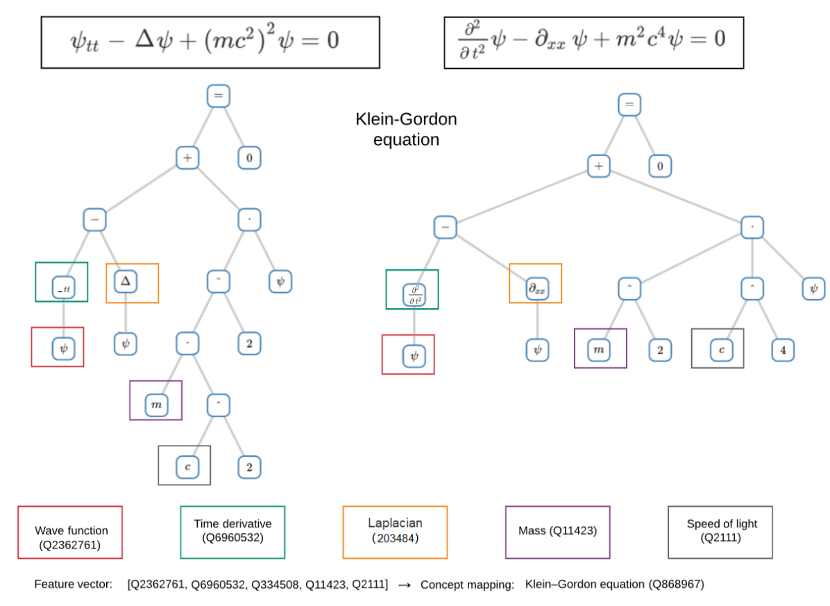
Figure 3: Comparison of two representations of the Klein–Gordon equation (left and right). Different constituents of the expression trees are marked as semantic entities that have a unique Wikidata ID (Qxxx).

Figure 3 shows the expression trees of two representations of the Klein–Gordon equation (left and right) in comparison. Different constituents of the equations are marked in the trees as semantic entities. They can be matched to unique IDs in a semantic database, e.g., Wikidata. For example, the identifier $c$ representing the ‘speed of light’ is assigned the Query ID (QID) ‘Q2111’. Since both trees contain the same semantic entities, they can be matched as representing the same Formula Concept.

Summarizing, we derive the following Formula Concept Retrieval system requirements from the identified challenges for FCD:

1. Set up a Formula Concept Database (FCDB);

2. Employ equivalence transformations and Computer Algebra Systems;

3. Enable Formula Concept Discovery by Recognition (FCD by FCR); and

4. Integrate formula matching via semantic formula encoding.

3.6 Conclusion (FCD)

We compare the effectiveness of retrieving different Formula Concept representations of Method 2 ($k$-Nearest-Neighbors in formula vector space) with Method 3 (Wikipedia article first formula multi-language heuristic). While Method 3 achieves a precision of 34% for retrieving Formula Concept representations from multilingual Wikipedia articles, Method 2 outperforms this with a precision of 68% using machine learning. The $k$NN approach is not only performing well, but it also has the advantage of being easily usable and transferable to other corpora. Method 1 can not be compared to the other two because it is a priori unclear where (at which number of webpages or textbooks) to stop the search. Therefore, we only concentrate on our three Formula Concept examples (KGE, EFE, and ME), for which we can retrieve a total of more than 30 representations, searching in publications, Wikipedia, and a textbook. We conclude that for Formula Concept Discovery to achieve the best results (retrieval of a large number of equivalent formula representations per concept), it is beneficial to combine the different methods optimally.

4 Formula Concept Recognition

In this section, we introduce methods for Formula Concept Recognition (FCR). Recall that the goal of FCR is to recognize formulas in documents as being instances of a previously defined Formula Concept.

The presented FCR methods were not introduced or published before. Prior work only included the first FCD experiments and results. Currently, to the best of our knowledge, no other FCR methods have been published so far. However, to establish comparability and replicability, we evaluate the performance of our approaches against that of open source and commercial formula search engines in Experiment 1 as presented in Section 4.1.

In the following, we describe and evaluate several different approaches for FCR. To assess the feasibility and performance of the proposed methods, we set up the following three experiments:

1. [Experiment 1:]

2. Formula Concept Search;

3. Formula Concept Classification and Clustering;

4. Formula Concept Similarity.

In Experiment 1, we investigate how well Formula Concepts can be retrieved by search queries using the formula LaTeX string or the formula constituents. Therefore, we employ several sources, such as Wikidata items, as well as Wikipedia articles and arXiv documents from the NTCIR dataset. The results from Wikidata can be associated with a unique semantic ID (the Wikidata QID). We compare the performance of the open source retrieval to selected competitor (formula) search engines. In Experiment 2, we assess how well a manually labeled balanced dataset of 100 Formula Concept examples from 10 classes can be automatically recognized by machine learning classification and clustering to separate the Formula Concepts in several vector encoding spaces. In Experiment 3, we test how well formula (encoding) similarities can indicate that different formulas are representations of the same Formula Concept. Therefore, we compute a similarity map matrix of pairwise formula or class similarities. The developed algorithms, the dataset, and full result tables are available at https://github.com/ag-gipp/formula-concept-retrieval.

4.1 Experiment 1: Formula Concept Search

We first approach the recognition of Formula Concepts (FCR) as a search ranking problem, in contrast to classification and clustering, examined in the subsequent experiment. To evaluate finding, i.e., recognizing FCs in large corpora of mathematical content, we employ three open data sources (Wikidata, Wikipedia, arXiv) and two methods (retrieval using formula LaTeX string or constituents). Furthermore, we compare the performance of our methods to two formula search engines, one open source (Approach0), and one commercial (Google).

Table 4: Ten classes of our test set with 100 Formula Concept differential equation examples, including a linked Wikidata QID and concept name with Wikipedia article source link (above), as well as an example equation LaTeX string.

Nr.	QID	Label	Name
1	Q868967	KGE	Klein–Gordon equation
2	Q273711	EFE	Einstein’s field equations
3	Q51501	ME	Maxwell’s equations
4	Q165498	SE	Schrödinger equation
5	Q860615	HE	Helmholtz equation
6	Q859808	BE	Biharmonic equation
7	Q104212301	NSL	Newton’s second law of motion
8	Q44746	HUP	Heisenberg uncertainty principle
9	Q177045	SLT	Second law of thermodynamics
10	Q83152	CL	Coulomb’s law

Label	Example Equation
KGE	u_{tt} + A u + f(u) = 0
EFE	G_{\mu \nu} = \kappa T_{\mu \nu}
ME	\text{div} \vec{E} = 4 \pi \rho
SE	\hat H}|\Psi\rangle = E |\Psi\rangle
HE	(\nabla^2 - k^2) A = -f
BE	\nabla^4\varphi=0
NSL	\vec{F} = \frac{d\vec{p}}{dt}
HUP	\sigma_{x}\sigma_{p} \geq \frac{\hbar}{2}
SLT	\oint \frac{\delta Q}{T} = 0
CL	|F| = \\frac{|q_1 \\times q_2|}{r^2}

For this and all subsequent FCR experiments, we collect a test set with 100 Formula Concept example differential equations from 10 classes. Table 4 shows the concept class names and labels, together with the corresponding Wikidata QID (above) and example LaTeX string (below). The linked Wikipedia article is the source of the respective equations, which we collected for each class. A full list of all 100 collected equations can be found in the appendix. The selection extends the three classes discussed in Section 3.3 by additional 7 classes with 10 examples each. Each class corresponds to a Wikipedia article (as indicated in Table 4). This means that we here apply the definition of a Formula Concept as a set of equation representations collected from the same Wikipedia article.

For each of our 100 example formulas, we evaluate the performance of 8 selected Formula Concept search retrieval sources: arXiv LaTeX, arXiv constituents, Wikidata LaTeX, Wikidata constituents, Wikipedia LaTeX, Wikipedia constituents, Approach0, and Google. The first 6 represent our retrieval methods over open corpora, while the last 2 employ search engines. The method label LaTeX indicates that the formulae are compared by their LaTeX strings, whereas ‘constituents’ means that the formula parts are aligned (set intersections of operators and identifiers).

We generated the top 10 results for each of the 8 sources on our 100 examples and manually assessed the ranking of the correct result for the resulting $10\times 8\times 100=8,000$ formulae. As ranking measures, we used ‘Top10 Recall’ and ‘Top1 Recall’ as well as ‘Mean Rank’ (MR) and ‘Mean Reciprocal Rank’ (MRR), which is defined as Voorhees (1999)

$$\text{MRR}=1/\text{MR}=\frac{1}{|Q|}\sum_{i=1}^{|Q|}\frac{1}{\text{rank}_{i}},$$

summing over all query results Q = 10. In this formula, $\text{rank}_{i}$ refers to the rank position of the first relevant document for the i-th query. The reciprocal value of the mean reciprocal rank represents the harmonic mean of the ranks.

Table 5: FCR as Formula Concept Search problem. Several open corpus sources (Wikidata and NTCIR Wikipedia, arXiv) are employed to retrieve formulas from a test set of 100 differential equations either using their LaTeX string or constituents. The performance is compared in several ranking metrics (MRR, etc.) to competitors, an open source (Approach0), and a commercial (Google).

Source / Metric	MRR	MR	Top10 Recall	Top1 Recall
Formula Concept Retrieval methods (FCRs)
arXiv LaTeX	0.70	2.38	0.48	0.27
arXiv constituents	0.71	2.91	0.11	0.07
Wikidata LaTeX	0.75	2.28	0.68	0.44
Wikidata constituents	0.54	2.65	0.17	0.05
Wikipedia LaTeX	0.78	1.78	0.74	0.48
Wikipedia constituents	0.66	2.70	0.40	0.21
Search Engines (SEs)
Approach0	0.64	2.59	0.44	0.21
Google	0.63	2.85	0.55	0.26
FCRs vs. SEs
Mean (FCRs)	0.69	2.45	0.43	0.25
Mean (SEs)	0.63	2.72	0.50	0.24

Table 5 shows the results of the Formula Concept search evaluation. The performance of different FCR methods is compared to state-of-the-art (formula) search engine competitors (Approach020 and Google21). We also tested other formula search engines, such as MathWebSearch, , zbMATH Open formulae, and Wolfram Alpha but they were either not working, access-restricted or too low performing to be included in the result table. The best results (lowest Mean Rank MR, highest Mean Reciprocal Rank MRR, and Recall) are marked in bold. The results exhibit that the FCR method source ‘Wikipedia LaTeX’ outperformed all other method sources in all metrics. This can be explained by the fact that our FCR examples were extracted from Wikipedia articles. However, not all equations were present in the NTCIR Wikipedia dataset. We find that the formula LaTeX string retrieval outperformed the retrieval using formula constituents. Furthermore, we compare our retrieval methods (FCRs) to the selected search engines (SEs). Our methods outperform the search engines in all metrics except ‘Top10 Recall’ (it is very close in the ‘Top1 Recall’ metrics). Summarizing, we compare the performance of different retrieval methods and sources in several ranking measures to demonstrate that it is possible to recognize Formula Concepts using search with a Mean Rank of down to 1.78, Mean Reciprocal Rank up to 0.78, and Recall up to 0.74. Our FCR methods outperform state-of-the-art search engines.

4.2 Experiment 2: Formula Concept Classification and Clustering

To assess how well the computer could separate our 100 Formula Concept examples into classes, we examine their joint formula (content or semantic) space. Recall that the formula content was defined following Scharpf et al. (2018) as the sets of operators, identifiers, and numbers that a formula contains. Because of Challenge 3 (substitutions) and Challenge 3 (different unit systems), we decided to neglect the set of numbers. Compared to the operators and identifiers, there are significantly fewer numbers, and they heavily depend on substitutions and unit systems (e.g., the number $8$ in the factor $8\pi$ or the exponents $4$ in (23)).

Since formulas in mathematics can be similar to each other syntactically, yet address completely different concepts semantically or vice versa, we analyze the relationship between syntactic and semantic encodings. There are two challenging cases: (1) syntactically similar but semantically different formulas (syntactic inter-class coherence but semantic inter-class separability) and (2) syntactically different but semantically coherent formulas (syntactic inner-class separability but semantic inner-class coherence). An example for (1) from our selected classes can be:

$$a\ \Psi_{t}+b\ \nabla^{2}\Psi+c\ \Psi=0\ \text{(class KGE) vs.}\ a\ \Psi_{tt}+b\ \nabla^{2}\Psi+c\ \Psi=0\ \text{(class SE)}$$

or

$$-\partial\Psi/\partial t^{2}+\nabla^{2}\Psi-m^{2}\Psi=0\ \text{(KGE) vs.}\ i\partial\Psi/\partial t+1/2m\nabla^{2}\Psi-V\Psi=0\ \text{(SE)}.$$

An example for (2) can be: $F=ma$ vs. $F=p/t$ (class NSL expressed using mass $m$ and acceleration $a$ vs. momentum $p$ and time $t$).

Encoding and classifying the syntactic or semantic formula content is indispensable, since the surrounding text is often noisy and the formula concepts are not explicitly named or described. Some authors of mathematical content implicitly assume the reader’s profound background knowledge. This limits the use of text-based encoding and classification methods. In the following, we describe and discuss our tests of the content vs. semantic coherence of Formula Concepts in terms of separability (classification accuracy and cluster centroid distance and purity).

For the machine learning experiments, we create four files with the equation labels, LaTeX strings, content, as well as semantic annotations, including Wikidata QIDs. Each of the files has 100 lines corresponding to the individual formulas, i.e., (10 Formula Concept examples from each of the 10 classes KGE EFE, ME, etc. respectively, see Table 4). As an example, consider the first formula (12). It belongs to the first class, so the line in the label file reads EFE. In the LaTeX string file, the corresponding line reads

\frac{1}{c^2}\frac{\partial^2 \psi}{\partial t^2} - \nabla^2\psi + \left(\frac{m_0 c}{\hbar} \right)^2\psi = 0.

The content line, containing the set of parsed operators and identifiers, then reads

c, \partial, \psi, t, \nabla, m, \hbar.

We encode their semantics as

c: "speed of light" (Q2111), \partial: "partial derivative" (Q186475), \psi: "wave function" (Q2362761), t: "time" (Q11471), \nabla: "del" (Q334508), m: "mass" (Q11423) , \hbar: "Planck constant" (Q122894)

where the ID in parenthesis is the unique QID from the item, we find in the semantic knowledge base Wikidata.

Summarizing, the data pipeline is the following: We parse the formula LaTeX strings (‘formula TeX’) to formula constituents (‘formula content’) and annotate them (‘formula semantics’) to get Wikidata encodings (‘formula qids’). The yields a dictionary of formula constituent meanings with an average of 2 different annotations per constituent. As an example, the identifier ‘R’ appears as ‘distance (Q126017)’ or ‘Ricci curvature’ (Q1195879)’.

In our experiment, we employ the following formula vector encodings of both operators and identifiers:

• Formula content TF-IDF;

• Formula content Doc2Vec;

• Formula semantics TF-IDF; and

• Formula semantics Doc2Vec.

For the formula content encodings, the sets of the parsed operator and identifier LaTeX strings from the content file are employed. For the formula semantics encodings, we use the sets of Wikidata QIDs. It is important to note that while the sequence of formula constituents does not matter for the TF-IDF encoding, it is considered by the Doc2Vec encoding. In our experiments, we focus on a relative evaluation, i.e., a comparison of different encodings, rather than optimizing the overall performance by tuning hyperparameters.

30 Examples

We first examine the separation of the three Formula Concepts by investigating the formula space in each of the four computed formula vector encodings. Figures 4 and 5 show the resulting plots. We reduce the dimensions via Principal Component Analysis (PCA) to two ($x$- and $y$-axes). Furthermore, we color-code the results of our formula clustering experiment (see next paragraph), such that each datapoint color corresponds to a different cluster computed by $k$-means ($k=3$) clustering. Apparently, in the formula content space with Doc2Vec encodings (second plot), the three Formula Concept classes are separated best with the largest distances between the three cluster centroids (see Table 6). Only two Formula Concept examples of class ME are incorrectly located in the cluster, which primarily consists of class KGE. We can identify these as being equation (35) and (36). We suspect the partial derivative to be causing the mix-up of these ME, since they predominantly occur in the KGE.

Table 6: Mean cluster centroid distance after employing PCA to reduce the number of datapoint dimensions to two (see the 2D plots in Figures 4 and 5). The formula content Doc2Vec encoding performs best (largest distance).

Encoding	Mean centroid distance
Formula content TF-IDF	0.57
Formula content Doc2Vec	0.81
Formula semantics TF-IDF	0.73
Formula semantics Doc2Vec	0.11

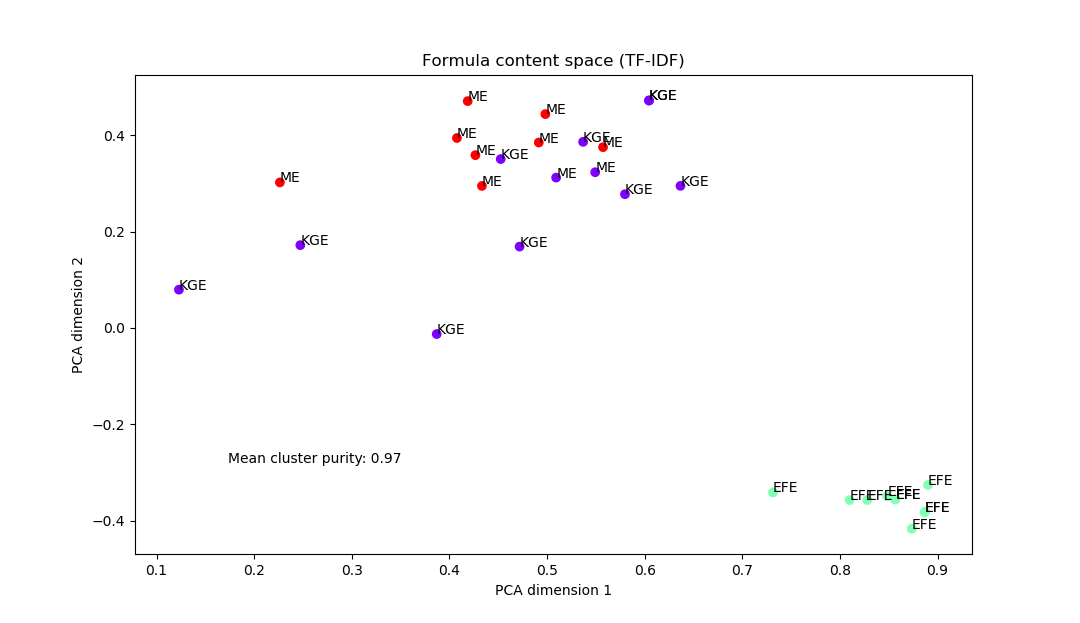
(a)

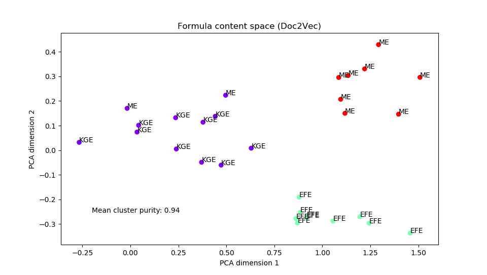
(b)

Figure 4: Formula content space of three selected Formula Concepts (KGE, EFE, ME), using TF-IDF or Doc2Vec encodings, reduced by Principal Component Analysis (PCA) to two dimensions. The color code corresponds to the clusters computed by $k$-means ($k=3$) clustering. The three classes are best separated in the formula content Doc2Vec encoding (second plot) with cluster mean centroid distance of $0.81$, purity of $0.94$, and classification accuracy of $0.90$.

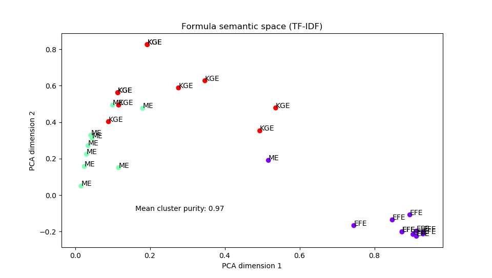
(a)

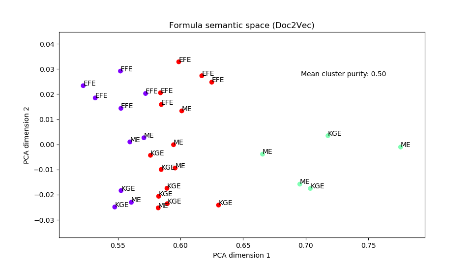
(b)

Figure 5: Formula semantic space of three selected Formula Concepts (KGE, EFE, ME), using TF-IDF or Doc2Vec encodings, reduced by Principal Component Analysis (PCA) to two dimensions. The color code corresponds to the clusters computed by $k$-means ($k=3$) clustering.

As another measure for the separability of our three example Formula Concepts, we calculate the cluster purity as the number of datapoints of the class that makes up the largest fraction of a cluster divided by the cluster size, averaged over all clusters:

$$\text{purity}=\underset{\text{clusters}}{\text{mean}}\left[\frac{1}{\text{cluster size}}\ \text{max}(\text{\#datapoints in cluster per class})\right].$$

​​Table 7 holds the cluster purities of a $k$-means clusterer on different formula vector encodings. Apparently, the formula content Doc2Vec encoding outperforms the others. This is illustrated by comparing Figures 4 and 5. In the Doc2Vec encoding, the smallest number of Formula Concept labels (only two) are mixed up.

Table 7: Mean cluster purity of a $k$-means clusterer on different formula vector encodings. The formula content Doc2Vec encoding performs best (highest purity).

Encoding	Mean cluster purity
Formula content TF-IDF	0.97
Formula content Doc2Vec	0.94
Formula semantics TF-IDF	0.97
Formula semantics Doc2Vec	0.50

As the third measure for the separability of our three example Formula Concepts, we calculate the classification accuracy of a Support Vector Machine (SVM) classifier on our four formula vector encodings. Summarizing, we test FCR approaches for Formula Concept separation using machine learning techniques such as neural formula vector encodings (Doc2Vec), dimensionality reduction (PCA), clustering ($k$-means), and classification (SVM). Our three measures of separability are 1) mean cluster centroid distance, 2) mean cluster purity, and 3) classification accuracy (cross-validated). While the formula semantic TF-IF encoding performs best (averaged over the two classifiers and cross-validation splittings), the formula content Doc2Vec encodings outperform the others in both cluster centroid distance and purity.

We avoid data skewness by employing a balanced dataset of examples equally distributed over classes.

The Formula Concept clustering using a $k$-means algorithm can assign 29/30 $\simeq$ 97% correctly, while the fuzzy string matching performs slightly worse with 28/30 $\simeq$ 93%. Random sampling only reaches 8/30 $\simeq$ 27%. So, the clustering outperforms the other methods. However, this only works if the cluster number $k$ (number of Formula Concept classes in the dataset) is known a priori.

100 Examples

In the next step, we extend our study to the full dataset of 100 examples FCs from 10 classes.

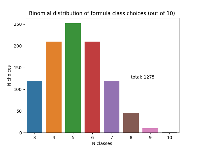
(a)

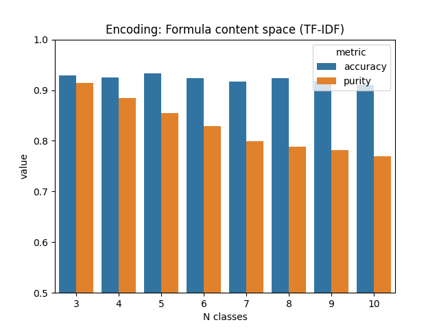
(b)

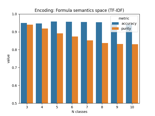
(c)

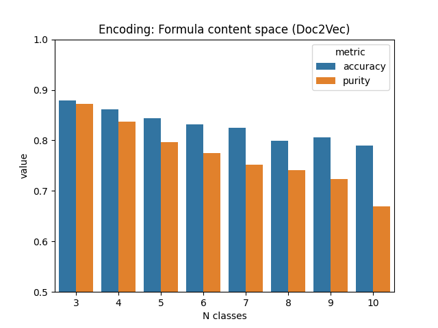
(d)

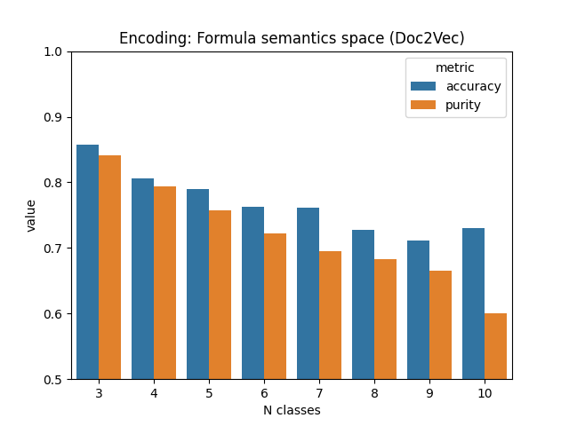
(e)

Figure 6: Classification accuracies (cross-validated) and cluster purities (labeling-referenced) for a selection of 100 equations, semantically annotated (constituent QIDs) and sorted into 10 classes (formula QIDs). The binomial choice distribution for a selection of $N$ formulas out of the pool is shown above. Four different encodings (Content TF-IDF, Semantics TF-IDF, Content Doc2Vec, and Semantics Doc2Vec) are compared below.

Table 8: Classification accuracies (cross-validated) and cluster purities (labeling-referenced) for a selection of 100 equations, semantically annotated (constituent QIDs) and sorted into 10 classes (formula QIDs). The binomial choice distribution for selecting $N$ formulas out of the pool is featured in the first two columns. Four different encodings (Content TF-IDF, Semantics TF-IDF, Content Doc2Vec, and Semantics Doc2Vec) are compared.

Classes	Choices	Metric	Cont. TF.	Cont. D2V.	Sem. TF.	Sem. D2V.
3	120	accuracy	0.93	0.95	0.88	0.86
3	120	purity	0.91	0.94	0.87	0.84
4	210	accuracy	0.93	0.95	0.86	0.81
4	210	purity	0.88	0.92	0.84	0.79
5	252	accuracy	0.93	0.96	0.84	0.79
5	252	purity	0.86	0.89	0.80	0.76
6	210	accuracy	0.92	0.96	0.83	0.76
6	210	purity	0.83	0.87	0.77	0.72
7	120	accuracy	0.92	0.96	0.82	0.76
7	120	purity	0.80	0.85	0.75	0.69
8	45	accuracy	0.92	0.95	0.80	0.73
8	45	purity	0.79	0.84	0.74	0.68
9	10	accuracy	0.92	0.94	0.81	0.71
9	10	purity	0.78	0.83	0.72	0.67
10	1	accuracy	0.91	0.94	0.79	0.73
10	1	purity	0.77	0.83	0.67	0.60
Mean	/	accuracy	0.92	0.95	0.83	0.77
Mean	/	purity	0.83	0.87	0.77	0.72

Figure 6 and Table 8 show the performance evaluation of classification (cross-validated) and clustering (labeling-referenced) of the labeled selection of 100 FC examples from 10 FC classes. Classification accuracy (blue bars) and cluster purity (orange bars) is computed for each encoding (content or semantics in TF-IDF or Doc2Vec) in all 1275 combinatoric class choices individually (with $N$ ranging from 3 to 10, see the top plot for the binomial distribution). The displayed values ($y$-axis) are averaged over all respective combinations for a given number of class choices ($x$-axis). For each of the 4*1275 runs, we perform N-fold cross-validation retrieving the classification accuracy.

For the TF-IDF encoding (upper plots), the results are the following: While the classification accuracy remains approximately stable with increasing N, the cluster purity decreases. This means that in the supervised retrieval case (FCR), clustering is most appropriate for a small number of classes. However, it can still be helpful in the unsupervised case for discovering (FCD) and labeling unknown classes. For the Doc2Vec encoding (lower plots), the results are the following: The classification accuracy also decreases with increasing N, and the cluster purity more strongly. This means that it might be preferable to employ TF-IDF instead of Doc2Vec, which even has the additional advantage of being faster to compute.

We conclude that the classification is potentially more useful than the clustering for labeled FCR (if the formulas are already annotated). Yet, also for unlabeled formulas, the clustering might not be helpful because, as stated before, the cluster number of different concepts is not known a priori. However, in the upcoming Experiment 3, we showed that a formula similarity map could be used instead as a means for both FCD and FCR.

4.3 Experiment 3: Formula Concept Similarity

In this experiment, we investigate the FC separability using FC similarity map matrices. We start with a preliminary analysis of the small set of 30 examples to be subsequently extended to all 100 examples.

30 Examples

Figure 7 shows the matrix of Formula Concept LaTeX fuzzy string similarities for the small selection of 30 formulas discussed in Section 3.3. We employ the fuzz.partial_ratio function of the Python package fuzzywuzzy. Each square corresponds to the similarity percentage of the example equation with the number displayed on the $x$-axis to the example equation with the number displayed on the $y$-axis. Since pairwise similarities are symmetric, the matrix is symmetric, and we can concentrate the investigations only on the part above or below the diagonal.

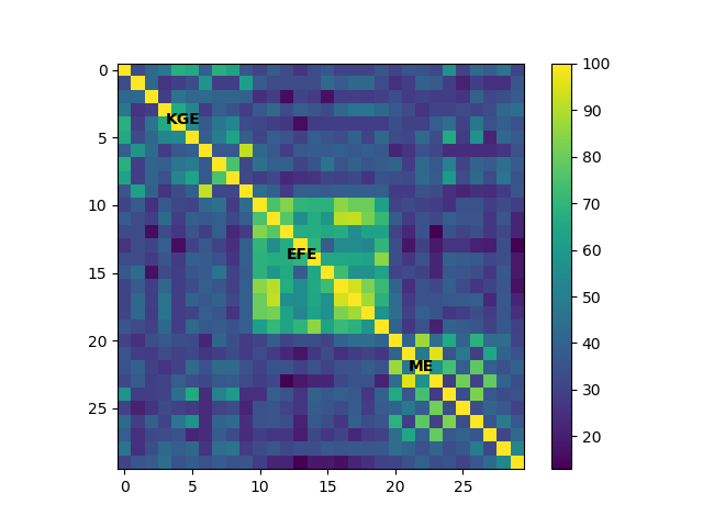
Figure 7: Matrix of the Formula Concept LaTeX fuzzy string similarity percentages. On the $x$- and $y$-axes, the equation number is displayed such that each little square corresponds to one similarity value between one equation and another.

Apparently, the three Formula Concepts (KGE equation number 1-10, EFE number 10-20, ME 20-30) form three large squares (or triangles) aligned on the diagonal (containing the individual 100% self-similarities). Particularly striking is the EFE square in the center of the matrix with its high values and density. This means that the Einstein Field Equations are the most similar, and the Formula Concept is highly coherent. The considered representations of the other two Formula Concepts are much more diverse and more difficult to match or identify. Figure 8 shows the matrix of the Formula Concept semantic similarities. The color code corresponds to the number of matching Wikidata QIDs of the corresponding Formula Concept examples (the $x$- and $y$-axes).

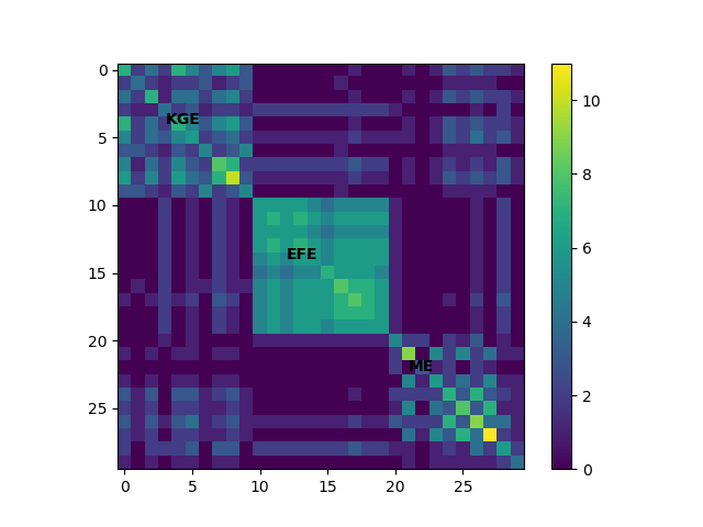
Figure 8: Matrix of the matching numbers of formula semantic QIDs. On the $x$- and $y$-axes, the equation number is displayed such that each square corresponds to one similarity value between one equation and another.

The distribution is very similar to the fuzzy LaTeX string content matching shown in Figure 7 (except the EFE square is slightly more distinct). Thus, semantification has no significant advantage here. However, in cases where the identifier symbols vary more, we expect an improvement.

100 Examples

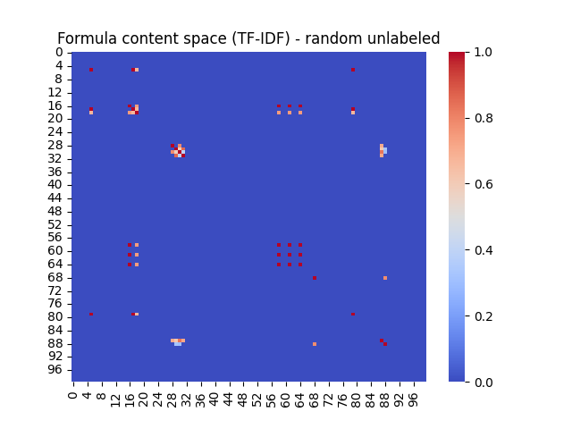
(a)

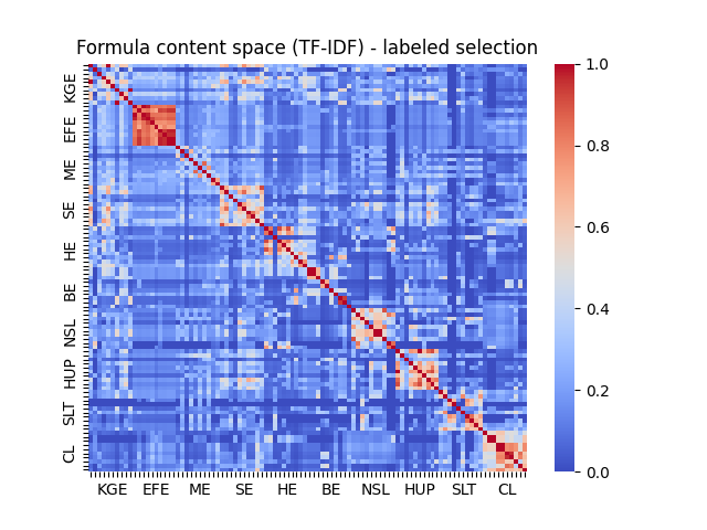
(b)

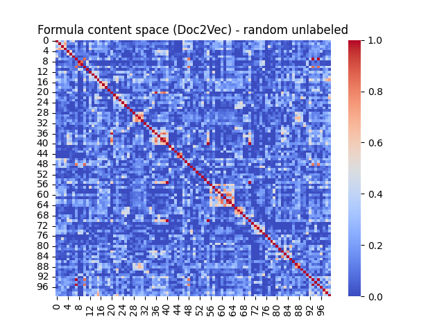
(c)

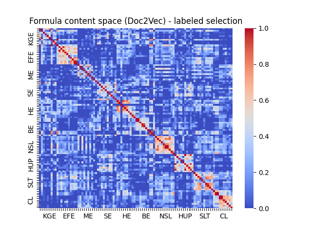
(d)

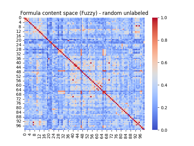
(e)

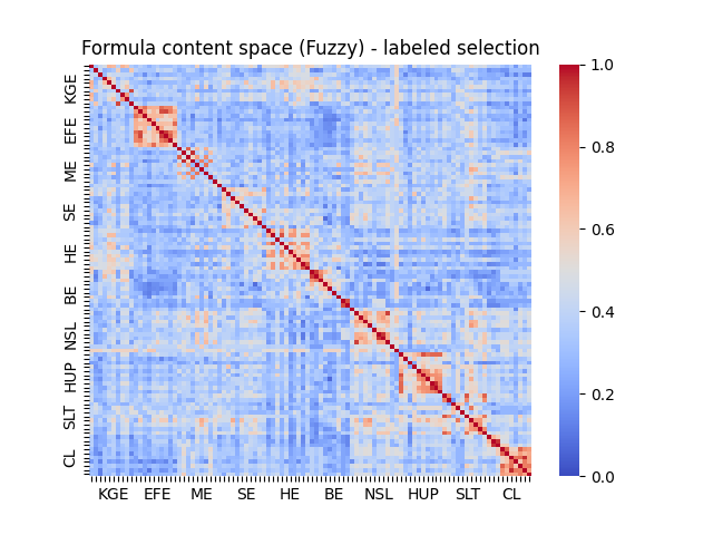
(f)

Figure 9: Comparing unlabeled random equations (left) from the arXiv NTCIR dataset (astro-ph domain) to selected labeled equations (right) annotated by a human domain expert in different encodings (TF-IDF above, Doc2Vec middle, Fuzzy below, Content left, and Semantic right). Axes show random numbers or selected equation class labels. Very high TF-IDF, Doc2Vec cosine, or fuzzy string similarity between equations are marked in red. Figure best viewed in color.

Figure 9 shows a comparison of the formula similarities of random unlabeled to all of our 100 selected labeled example formulas. While the random formulas are extracted from the arXiv NTCIR dataset, the labeled selection is taken from Wikipedia articles.

In Doc2Vec and Fuzzy encodings, the random unlabeled similarity map appears to be very similar to that of the labeled selection. This indicates that in both random sampling and labeled sampling, most of the formulas are not very similar to each other (blue background). However, for the labeled selection, there is an apparent self-coherence of the individual labeled FC classes (brighter red squares on the diagonal line).

We conclude that since the similarity map of labeled FCs is not weaker (less similarity) than that for random formulas, we can justify the classification and clustering as an appropriate tool or suitable means to recognize FCs. The lack of similarity or distinctness of the labeled classes does reflect the real-world situation for formulas in corpora, which is fortunate since it makes search and machine learning methods effective.

We can show that in the random sampling, the formula distinctness (low similarity) is equally low as for the labeled selection. This means that our machine learning experiments presented in Section 2 are reasonable since they represent an information retrieval scenario that could occur.

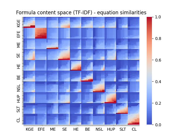
(a)

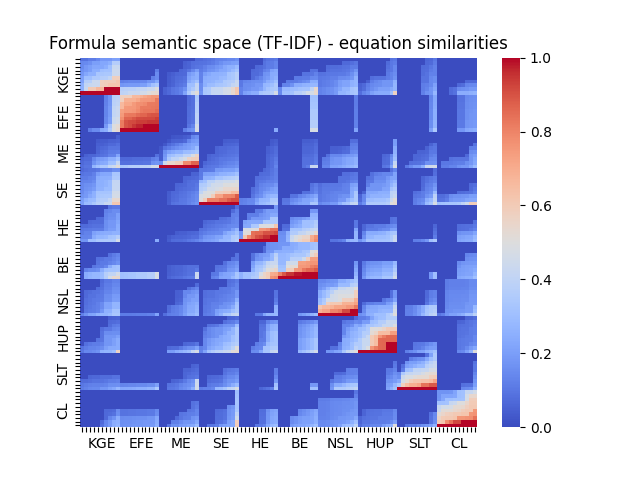
(b)

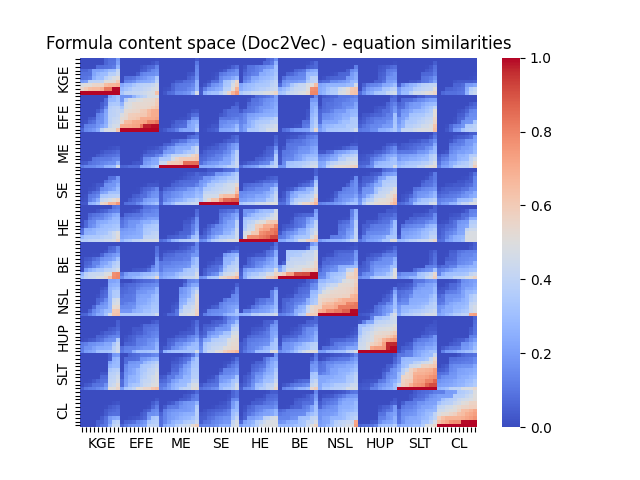
(c)

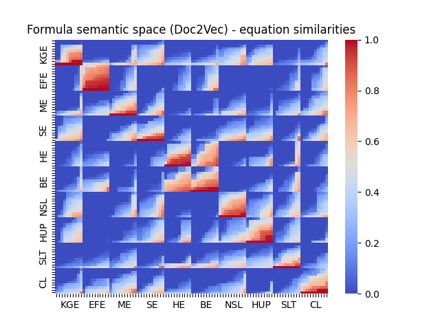
(d)

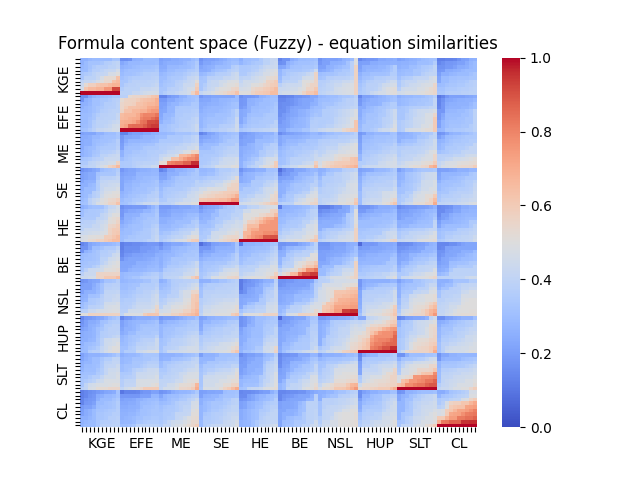
(e)

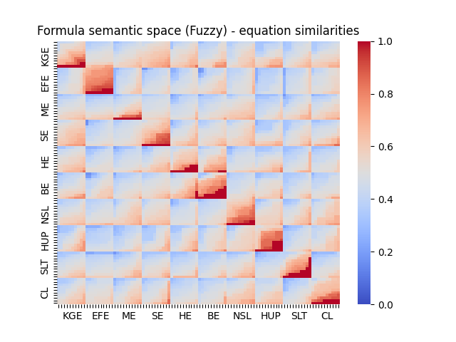
(f)

Figure 10: Comparing labeled equation similarities for different encodings (TF-IDF above, Doc2Vec middle, Fuzzy below, Content left, and Semantic right). Axes show equation class labels. Very high TF-IDF, Doc2Vec cosine or fuzzy string similarity between equations are marked in red. Similarities are sorted within classes. Figure best viewed in color.

Figure 10 shows the formula similarities in different encodings (TF-IDF, Doc2Vec, Fuzzy) for all 100 examples, comparing the content space (formula constituent symbols encoded) to the semantic space (formula constituent QIDs encoded). Similarities are sorted within classes. The self-coherence of the labeled formula classes (labels on axes) is evident in all encodings. However, in the semantic space (Doc2Vec) encoding, additional inter-class / cross-class coherences are visible (some squares span several classes, e.g., ‘BE’ and ‘HE’ in the middle). This indicates latent semantic coherences that are less visible in the unsemantified content encoding.

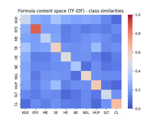
(a)

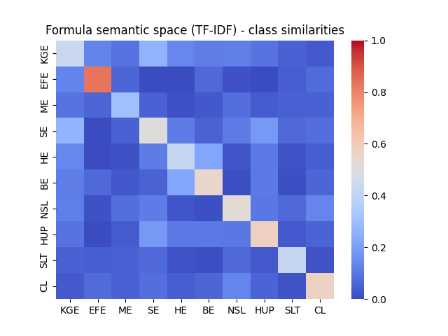
(b)

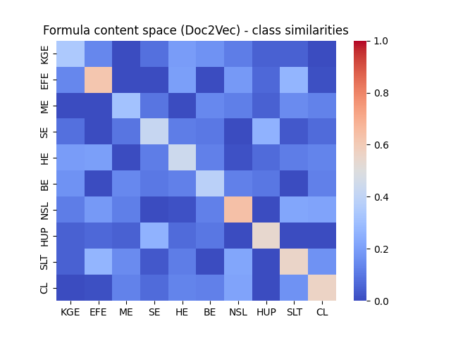
(c)

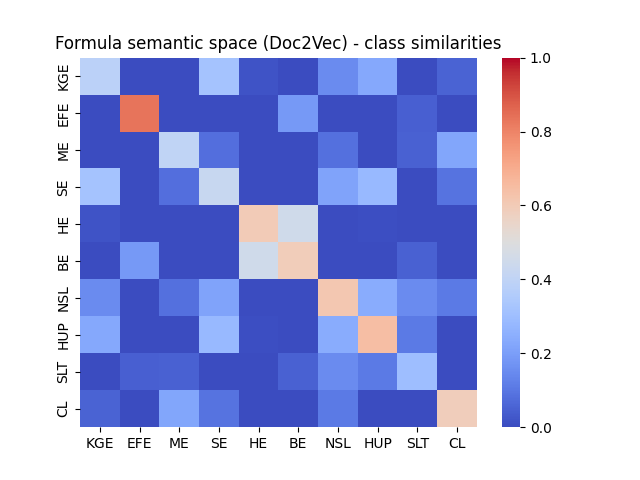
(d)

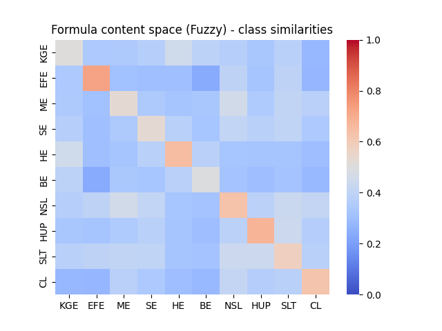
(e)

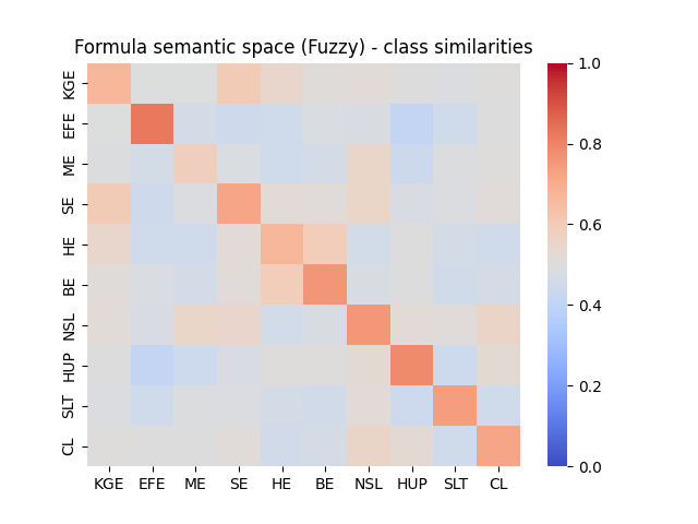
(f)

Figure 11: Comparing labeled averaged class similarities for different encodings (TF-IDF above, Doc2Vec middle, Fuzzy below, Content left, and Semantic right). Axes show equation class labels. Very high TF-IDF, Doc2Vec cosine or fuzzy string similarity between equations are marked in red. Figure best viewed in color.

Figure 11 shows the formula similarities in different encodings and spaces averaged over classes (mean pooling). This view helps to better highlight the intra-class and inter-class coherences. On the top-left, the high intra-class coherence of the ‘EFE’ formulas is illustrated by the prominent darker (more red intense) square. Moreover, the cross-class coherence mentioned in the description of Figure 10 is apparent again in the semantic space (Doc2Vec) encoding shown in the center of the middle right plot. Besides, other class similarities, such as that of the Klein–Gordon equations (‘KGE’) and Schrödinger equations (‘SE’), can be identified as brighter squares. Notice that the semantic (Fuzzy) space map (Figure 10 bottom right) shows that the inter-class similarity between KGE and SE in the semantic space is comparably high as the intra-class similarity of the ME class. This is reasonable, since they are indeed semantically very close. In the quantum physics framework, one equation can be derived from the other and vice versa. On the other hand, the intra-class similarity of the ME instances is high, since they are mutually semantically related. The FC class similarity maps are also helpful for FCD, discovering FCs as coherent similarity areas to be subsequently analyzed and labeled.

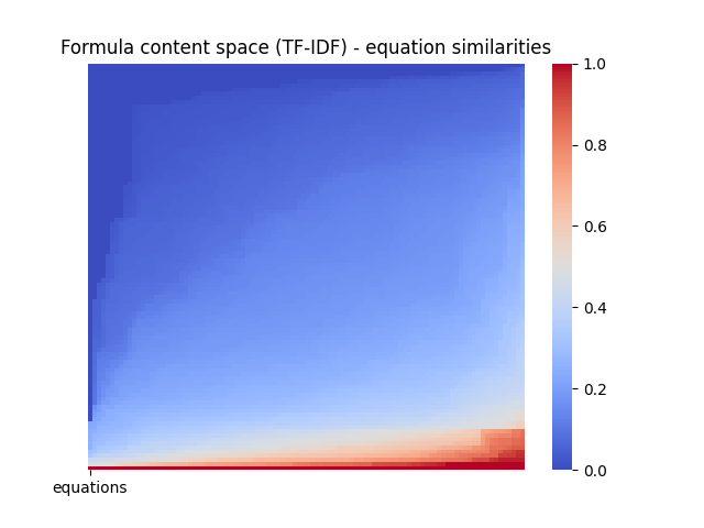
(a)

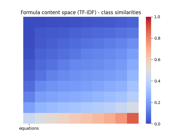
(b)

Figure 12: Sorted similarity maps (Content TF-IDF encoding) for equations (left) and classes (right). The mean equation similarity is 0.2.

Figure 12 illustrates the overall dissimilarity of the equations in a sorted similarity map. The blue space (low similarity) significantly outweighs the red area (high similarity) at the bottom. The low mean equation similarity of 0.2 motivates FCR methods to exploit the separability.

4.4 Conclusion (FCR)

In three different experiments, we investigate the feasibility and effectiveness of methods to retrieve, separate, and recognize Formula Concepts (FCR). For all experiments, we employ a manually labeled dataset of 100 Formula Concept examples from 10 classes retrieved from Wikipedia articles.

In Experiment 1 (Formula Concept search), we compare 8 different formula search methods on open corpora (Wikidata, Wikipedia, arXiv) and the web. We test how well Formula Concepts can be retrieved by search queries using either the formula LaTeX string or the formula constituents, respectively. The results show that using different retrieval methods and sources, it is possible to recognize Formula Concepts using search with a Mean Rank down to 1.78, Mean Reciprocal Rank up to 0.78, and Recall up to 0.74. Our FCR methods outperform the state-of-the-art search engines Approach0 and Google.

Experiment 2 (Formula Concept classification and clustering), we assess Formula Concept separability by machine learning classification and clustering in selected formula encodings. The results show while the cluster purity decreases with more FC classes, classification accuracy remains approximately stable around 0.9 when using TF-IDF formula encodings. This means that with stable accuracies, FC classification might be a more powerful means for FCR than FC clustering.

Experiment 3 (Formula Concept similarity), we visualize formula (encoding) separability in similarity map matrices to illustrate coherence and overlap of Formula Concepts. The results show that similarity maps are a valuable method for identifying both intra-class coherence and inter-class separability or overlap, which is useful for both FCD and FCR. Furthermore, the results motivate the employed machine learning methods since a comparison of our manual formula selection to randomly chosen formulas shows that in both cases, Formula Concepts are rather dissimilar and thus their classes separable from each other.

We conclude that the search for specific formulas within a large dataset of STEM documents is a challenging problem. Furthermore, we note that for FCR, there is an urgent need to augment semantic formula databases, for example, MathMLben and Wikidata, such that they allow for multiple representations of a formula to be stored as a Formula Concept. Having formulas tagged by Wikidata QIDs enables using them as markers in documents that can be cited (math citations). Additionally, they can be employed to improve content-based recommender systems for academic literature, plagiarism detection systems, and ontology learning.

Note that our study’s aim is not a large-scale evaluation but rather a deductive conceptual work. The data, plots, and results we presented serve to illustrate the methodological concepts. We demonstrate the fundamental feasibility using examples and outline the potential for machine learning on labeled formula data. For a large-scale analysis using unlabeled formula data, we refer to the literature Scharpf et al. (2020a); Greiner-Petter et al. (2020).

5 Future Work

This section outlines future endeavors and challenges, which we plan to address to further improve, evaluate, and apply FCD and FCR methods to additional use cases. These include exploring the practicability of a ‘Formula Rank’, investigating a formula semantics sufficiency hypothesis, and developing methods for efficient semantic formula and triple annotation.

FormulaRank and Semantic Indexing.

In analogy to Google’s ‘PageRank’ Brin and Page (1998), and ‘TextRank’
 Mihalcea and Tarau (2004), we propose to employ a ‘FormulaRank’ for Formula Concept popularity retrieval. FormulaRank is supposed to rank formulas by the number of neighbors ($k$NN) or constituent intersections to estimate their importance. For this experiment, we first need to elaborate on interpretation standards and evaluation metrics for the results. Secondly, we will develop and evaluate semantic indexing of the arXiv datasets containing formulas, their LaTeX string, constituents retrieved from MathML tags, surrounding text, and more.

Functional vs. Semantic Recognition.

Furthermore, we will investigate the following research question: “Does the recognition of Formula Concepts require to take the functional relations of the formulas into account, or is it sufficient to only consider the semantics of the formula constituents?”. As an example, the Klein–Gordon equation

$$\frac{1}{c^{2}}\frac{\partial^{2}\psi}{\partial t^{2}}-\nabla^{2}\psi+\left(\frac{m_{0}c}{\hbar}\right)^{2}\psi=0,$$

can be encoded as the semantic fingerprint of its constituents:

c: "speed of light" (Q2111), \partial: "partial derivative" (Q186475), \psi: "wave function" (Q2362761), t: "time" (Q11471), \nabla: "del" (Q334508), m: "mass" (Q11423) , \hbar: "Planck constant" (Q122894)

Alternatively, one could additionally take into account that the partial derivatives $\partial/\partial t$ and $\partial/\partial x$ act on the wave function $\psi$ and are applied with respect to both time $t$ and space $x$. Considering this circumstance would mean taking the functional relations of the formulas into account instead of merely considering the set of the semantics (fingerprint) of the formula constituents.

Semantic Annotations.

To enable FCD by FCR, we are building a LaTeX formula annotation recommender system Scharpf et al. (2019b), which helps and motivates authors from the STEM disciplines to make their papers semantically machine-interpretable by annotating formula and identifier names with Wikidata items (name and QID). We need labeled formula data for the semantic encodings and formula classification introduced in Section 4.2. Our long-term goal for this system is to directly integrate the annotation recommendation into both Wikipedia and Overleaf’s editing or composing views. This would allow the Wikipedia and research communities to be more easily included in the semantification process of mathematical articles and research papers. Employing extended AI-aided formula annotation enables scaling our approaches in further research projects on our infrastructure at Wikimedia, zbMATH Open, and the University of Göttingen.

RDF Triple Extraction.

In the future, the semantic annotator will provide recommendations of RDF triples, both for natural language and mathematical statements. A natural language statement can be, for example, the triple {theory of relativity (Q43514), instance of (P31), scientific theory (Q3239681)}. For the mathematical statements, the Formula Concepts are represented as the triple {Formula Concept item name, defining formula, formula LaTeX string}.

Conflict of Interest

The authors declare that they have no conflict of interest.

Appendix: Formula Concept Examples

Einstein Field Equations in Wikipedia (10 Results).

$$R_{\mu\nu}-\tfrac{1}{2}R\,g_{\mu\nu}+\Lambda g_{\mu\nu}=\frac{8\pi G}{c^{4}}T_{\mu\nu},$$

$$G_{\mu\nu}=R_{\mu\nu}-\tfrac{1}{2}Rg_{\mu\nu},$$

$$G_{\mu\nu}+\Lambda g_{\mu\nu}=\frac{8\pi G}{c^{4}}T_{\mu\nu},$$

$$G_{\mu\nu}+\Lambda g_{\mu\nu}=8\pi T_{\mu\nu}~{}(G=c=1),$$

$$R_{\mu\nu}-\tfrac{1}{2}Rg_{\mu\nu}-\Lambda g_{\mu\nu}=-\frac{8\pi G}{c^{4}}T_{\mu\nu},$$

$$R-\frac{D}{2}R+D\Lambda=\frac{8\pi G}{c^{4}}T,$$

$$-R+\frac{D\Lambda}{\frac{D}{2}-1}=\frac{8\pi G}{c^{4}}\frac{T}{\frac{D}{2}-1},$$

$$R_{\mu\nu}-\frac{\Lambda g_{\mu\nu}}{\frac{D}{2}-1}=\frac{8\pi G}{c^{4}}\left(T_{\mu\nu}-\frac{1}{D-2}Tg_{\mu\nu}\right),$$

$$R_{\mu\nu}-\Lambda g_{\mu\nu}=\frac{8\pi G}{c^{4}}\left(T_{\mu\nu}-\tfrac{1}{2}T\,g_{\mu\nu}\right),$$

$$R_{\mu\nu}-\tfrac{1}{2}R\,g_{\mu\nu}+\Lambda g_{\mu\nu}=\frac{8\pi G}{c^{4}}T_{\mu\nu}~{}\text{(duplicate)}.$$

Einstein Field Equations in arXiv NTCIR (77 Results).

$$G_{\mu\nu}-{1\over 2}Rg_{\mu\nu}=\kappa(T^{\varphi}_{\mu\nu}+T_{\mu\nu}),$$

$$R^{\mu\nu}-{1\over 2}g^{\mu\nu}(R-2\Lambda)=8\pi GT^{\mu\nu},$$

$$R_{\mu\nu}-\frac{1}{2}g_{\mu\nu}R+\Lambda_{c}g_{\mu\nu}=8\pi GT_{\mu\nu},$$

$$R_{\mu\nu}-{1\over 2}Rg_{\mu\nu}+\Lambda g_{\mu\nu}=8\pi GT_{\mu\nu},$$

$$G_{\mu\nu}=-\Lambda g_{\mu\nu}+\kappa^{2}T^{\rm tot}_{\mu\nu},$$

$$G_{AB}\equiv R_{AB}-{1\over 2}g_{AB}R=\kappa^{2}\,T_{AB},$$

$$G_{\mu\nu}+\Lambda g_{\mu\nu}=\kappa T_{\mu\nu},$$

$$G_{\mu\nu}-\Lambda g_{\mu\nu}=\kappa T_{\mu\nu},$$

$$G_{\mu\nu}-g_{\mu\nu}\Lambda=\frac{8\pi G}{c_{0}^{4}\phi^{4}}T_{\mu\nu},$$

$$R_{\mu\nu}-\frac{1}{2}Rg_{\mu\nu}+\Lambda g_{\mu\nu}=8\pi G\,T_{\mu\nu},$$

$$R_{\mu\nu}-{1\over 2}g_{\mu\nu}R=g_{\mu\nu}\Lambda-8\pi GT_{\mu\nu},$$

$$R_{\mu\nu}-\frac{1}{2}g_{\mu\nu}R+\Lambda g_{\mu\nu}=-8\pi GT_{\mu\nu},$$

$$R_{\mu\nu}-{1\over 2}g_{\mu\nu}R=\kappa T_{\mu\nu}-{\Lambda\over 2}g_{\mu\nu},$$

$$R_{\mu\nu}-{1\over 2}g_{\mu\nu}R=8\pi G[T_{\mu\nu}^{c}+T_{\mu\nu}^{q}],$$

$$R_{\mu\nu}-{1\over{2}}g_{\mu\nu}R=g_{\mu\nu}\Lambda-8\pi GT_{\mu\nu},$$

$$R_{\mu\nu}-{1\over 2}Rg_{\mu\nu}={8\pi G\over c^{4}}T_{\mu\nu},$$

$$R_{\mu\nu}-\frac{1}{2}g_{\mu\nu}R={\frac{8\pi G}{c^{4}}}T_{\mu\nu},$$

$$G^{\mu\nu}+\Lambda g^{\mu\nu}=\kappa{T_{e}}^{\mu\nu},$$

$$G^{\mu\nu}-T^{\mu\nu}=\kappa{T_{g}}^{\mu\nu},$$

$$R_{\mu\nu}-\frac{1}{2}Rg_{\mu\nu}+\Lambda g_{\mu\nu}=8\pi G\,T_{\mu\nu}~{}\text{(duplicate)},$$

$$R_{\mu\nu}-\frac{1}{2}g_{\mu\nu}R=8\pi G\,T_{\mu\nu}+\Lambda\,g_{\mu\nu},$$

$$G_{\mu\nu}+\Lambda g_{\mu\nu}=\kappa T_{\mu\nu},$$

$$R_{\mu\nu}-\frac{1}{2}g_{\mu\nu}R+\Lambda g_{\mu\nu}=8\pi GT_{\mu\nu},$$

$$G_{\mu\nu}=-\Lambda_{4}g_{\mu\nu}+\frac{1}{2\alpha_{0}}T_{\mu\nu}^{\rm c.c.},$$

$$R_{\mu\nu}-\frac{1}{2}g_{\mu\nu}R+\Lambda_{c}g_{\mu\nu}=8\pi GT_{\mu\nu},$$

$$R_{\mu\nu}-\frac{1}{2}~{}{}g_{\mu\nu}R=8\pi GT_{\mu\nu}-\Lambda g_{\mu\nu}~{}{},$$

$${G}_{\mu\nu}+\alpha{H}_{\mu\nu}+\Lambda g_{\mu\nu}=\kappa_{n}^{2}{T}_{\mu\nu},$$

$$R_{\mu\nu}-{1\over 2}Rg_{\mu\nu}=-\Lambda g_{\mu\nu}+8\pi GT_{\mu\nu},$$

$$G_{\mu\nu}+\Lambda_{\mathrm{R}}g_{\mu\nu}=8\pi G\langle\widetilde{T}_{\mu\nu}\rangle,$$

$$G_{\mu\nu}+\Phi_{\mu\nu}+\Lambda g_{\mu\nu}=\kappa T_{\mu\nu}~{}\text{(repeated 3 times)},$$

$$R_{(\mu\nu)}-\frac{1}{2}Rg_{\mu\nu}+\Lambda g_{\mu\nu}=\kappa T_{\mu\nu},$$

$$R_{\mu\nu}-{1\over 2}g_{\mu\nu}R=8\pi GT_{\mu\nu}+\Lambda g_{\mu\nu},$$

$$R_{\mu\nu}-\frac{1}{2}Rg_{\mu\nu}=\kappa_{r}(T)T_{\mu\nu}+\Lambda(T)g_{\mu\nu},$$

$$R_{\mu\nu}-\frac{1}{2}Rg_{\mu\nu}=\kappa(T_{\mu\nu}^{m}+T_{\mu\nu}^{\Lambda}),$$

$$R_{\mu\nu}-\frac{1}{2}Rg_{\mu\nu}=\kappa T_{\mu\nu}+\Lambda(T)g_{\mu\nu},$$

$$R_{\mu\nu}-\frac{1}{2}Rg_{\mu\nu}=\kappa_{r}T_{\mu\nu}+\Lambda(T)g_{\mu\nu},$$

$$K_{\mu\nu}-Kg_{\mu\nu}=-\frac{\kappa^{2}}{2}T_{\mu\nu}+r_{c}G_{\mu\nu},$$

$$R_{\mu\nu}-\frac{1}{2}g_{\mu\nu}R+\Lambda_{c}g_{\mu\nu}=\kappa T_{\mu\nu},$$

$$R_{\mu\nu}-\frac{1}{2}g_{\mu\nu}R+\Lambda g_{\mu\nu}=8\pi GT_{\mu\nu},$$

$$R_{\mu\nu}-\Lambda g_{\mu\nu}=8\pi G(T_{\mu\nu}-{1\over 2}g_{\mu\nu}T),$$

$$R_{\mu\nu}-{1\over 2}g_{\mu\nu}R+\Lambda\,g_{\mu\nu}=8\pi G_{N}\,T_{\mu\nu},$$

$$R_{\mu\nu}-\frac{1}{2}g_{\mu\nu}R=\frac{8\pi G}{c^{4}}T_{\mu\nu},$$

$$G_{\mu\nu}=R_{\mu\nu}-\frac{1}{2}g_{\mu\nu}R=8\pi GT_{\mu\nu}-\Lambda g_{\mu\nu},$$

$$R_{\mu\nu}-\frac{1}{2}\,Rg_{\mu\nu}=\kappa\,T_{\mu\nu}-\Lambda\,g_{\mu\nu},$$

$$R_{\mu\nu}-\frac{1}{2}g_{\mu\nu}R-\Lambda g_{\mu\nu}=(8\pi G_{N})T_{\mu\nu},$$

$$R_{\mu\nu}-\frac{1}{2}g_{\mu\nu}R+\Lambda g_{\mu\nu}=-\kappa T_{\mu\nu},$$

$$G_{\mu\nu}=\kappa_{4}^{2}T_{\mu\nu}-\Lambda g_{\mu\nu}+Q_{\mu\nu},$$

$$R_{\mu\nu}-\frac{1}{2}g_{\mu\nu}R=\frac{8\pi G}{c^{4}}T_{\mu\nu},$$

$$R_{\mu\nu}-\frac{1}{2}g_{\mu\nu}R+\Lambda g_{\mu\nu}=-8\pi GT_{\mu\nu}f_{R}\,G_{\mu\nu},$$

$$R_{\mu\nu}-\frac{1}{2}Rg_{\mu\nu}=8\pi GT_{\mu\nu}-\Lambda g_{\mu\nu}T^{\rm RG}_{\mu\nu},$$

$$R_{\mu\nu}-\frac{1}{2}g_{\mu\nu}R+\Lambda g_{\mu\nu}=8\pi GT_{\mu\nu},$$

$$E^{\mu\nu}=-G^{\mu\nu}+\kappa T^{\mu\nu}-\Lambda g^{\mu\nu},$$

$$G_{\mu\nu}=R_{\mu\nu}-g_{\mu\nu}R/2=\kappa T^{\mu\nu}-\Lambda g_{\mu\nu},$$

$$R_{\mu\nu}-\frac{1}{2}g_{\mu\nu}R=\frac{8\pi G}{c^{4}}T_{\mu\nu},$$

$$R_{\mu\nu}-\frac{1}{2}g_{\mu\nu}R=8\pi G_{5}T_{\mu\nu}-\Lambda_{5}g_{\mu\nu},$$

$$R_{\mu\nu}-{1\over 2}Rg_{\mu\nu}+\Lambda_{eff}g_{\mu\nu}=8\pi GT_{\mu\nu},$$

$$R_{\mu\nu}-{1\over 2}Rg_{\mu\nu}+\Lambda g_{\mu\nu}=8\pi GT_{\mu\nu},$$

$$R_{\mu\nu}-{1\over 2}g_{\mu\nu}R={8\pi G\over c^{4}}T_{\mu\nu},$$

$$R_{\mu\nu}-\frac{1}{2}g_{\mu\nu}R-g_{\mu\nu}\Lambda=8\pi GT_{\mu\nu},$$

$$G_{\mu\nu}+\Lambda g_{\mu\nu}=\frac{\kappa}{e^{2}}T_{\mu\nu},$$

$$R_{\mu\nu}-\frac{1}{2}\,g_{\mu\nu}\,R=8\pi GT_{\mu\nu}+\Lambda,$$

$$G_{\mu\nu}\equiv R_{\mu\nu}-\frac{1}{2}Rg_{\mu\nu}=\kappa^{2}T_{\mu\nu},$$

$$G_{\mu\nu}=R_{\mu\nu}-\frac{1}{2}Rg_{\mu\nu}=\kappa T_{\mu\nu},$$

$$G^{\mu\nu}=-\Lambda(x)g^{\mu\nu}+\kappa T^{\mu\nu}_{\rm M},$$

$$R_{\mu\nu}-{g_{\mu\nu}\over 2}R={8\pi G\over c^{4}}T_{\mu\nu}{1\over 2}{\rm Tr}H_{\chi}^{2},$$

$$R_{\mu\nu}-\frac{1}{2}g_{\mu\nu}R+\Lambda g_{\mu\nu}=\kappa T_{\mu\nu},$$

$$R_{\mu\nu}-\frac{1}{2}g_{\mu\nu}R+g_{\mu\nu}\Lambda=\kappa T_{\mu\nu},$$

$$G_{\mu\nu}-g_{\mu\nu}\Lambda={{8\pi G}\over c^{4}}T_{\mu\nu},$$

$$G_{\mu\nu}=R_{\mu\nu}-\frac{1}{2}g_{\mu\nu}R=\kappa^{2}T_{\mu\nu},$$

$$R^{\mu\nu}-\frac{1}{2}g^{\mu\nu}R=\frac{8\pi G}{c^{4}}T^{\prime\mu\nu},$$

$$R^{\mu\nu}-\frac{1}{2}g^{\mu\nu}R=\Lambda g^{\mu\nu}-8\pi GT^{\mu\nu}.$$

Differential Equation Concept Class Examples (100 from 10 classes).

$$\text{{Klein--Gordon Equation (KGE)}}:\hskip 71.13188pt$$

$$\frac{1}{c^{2}}\frac{\partial^{2}\psi}{\partial t^{2}}-\nabla^{2}\psi+\left(\frac{m_{0}c}{\hbar}\right)^{2}\psi=0,\hskip 71.13188pt$$

$$u_{tt}+Au+f(u)=0,\hskip 71.13188pt$$

$$\partial^{2}_{ct}h_{n}(z,t)-\partial^{2}_{z}h_{n}(z,t)+\nu_{n}^{2}h_{n}(z,t)=0,\hskip 71.13188pt$$

$$\nabla^{a}\nabla_{a}\psi=\mu^{2}\psi,\hskip 71.13188pt$$

$$-\hbar^{2}\frac{\partial^{2}\Psi}{\partial t^{2}}+c^{2}\hbar^{2}\nabla^{2}\Psi=m_{0}^{2}c^{4}\Psi,\hskip 71.13188pt$$

$$\nabla^{2}\phi-\frac{1}{c^{2}}\frac{\partial^{2}\phi}{\partial t^{2}}-\frac{2\alpha+\alpha}{c^{2}}\frac{\partial\phi}{\partial t}-\frac{\alpha^{2}+a\alpha}{c^{2}}\phi=0,\hskip 71.13188pt$$

$$u_{tt}-\Delta u+m^{2}u+G^{\prime}(u)=0,\hskip 71.13188pt$$

$$\left(\eta^{\mu\nu}\frac{\partial}{x^{\mu}}\frac{\partial}{x^{\nu}}-\left(\frac{mc}{\hbar}\right)^{2}\right)\varphi=0,\hskip 71.13188pt$$

$$\left(-\frac{1}{c^{2}}\frac{\partial^{2}}{\partial t^{2}}\sum_{i=1}^{p}\frac{\partial}{x^{i}}\frac{\partial}{x^{i}}-\left(\frac{mc}{\hbar}\right)^{2}\right)\varphi=0,\hskip 71.13188pt$$

$$u_{tt}-\Delta u+mu+P^{\prime}(u)=0.\hskip 71.13188pt$$

$$\text{{Einstein Field Equations (EFE)}}:\hskip 71.13188pt$$

$$G_{\mu\nu}+\Lambda g_{\mu\nu}=\kappa T_{\mu\nu},\hskip 71.13188pt$$

$$R_{\mu\nu}-\frac{1}{2}g_{\mu\nu}R-\Lambda g_{\mu\nu}=(8\pi G_{N})T_{\mu\nu},\hskip 71.13188pt$$

$$G_{\mu\nu}=-\Lambda g_{\mu\nu}+\kappa^{2}T^{\rm tot}_{\mu\nu},\hskip 71.13188pt$$

$$G_{\mu\nu}=R_{\mu\nu}-g_{\mu\nu}R/2=\kappa T^{\mu\nu}-\Lambda g_{\mu\nu},\hskip 71.13188pt$$

$$R_{\mu\nu}-\frac{1}{2}Rg_{\mu\nu}=\kappa_{r}(T)T_{\mu\nu}+\Lambda(T)g_{\mu\nu},\hskip 71.13188pt$$

$$K_{\mu\nu}-Kg_{\mu\nu}=-\frac{\kappa^{2}}{2}T_{\mu\nu}+r_{c}G_{\mu\nu},\hskip 71.13188pt$$

$$R_{\mu\nu}-\frac{1}{2}g_{\mu\nu}R+\Lambda g_{\mu\nu}=-8\pi GT_{\mu\nu}f_{R}G_{\mu\nu},\hskip 71.13188pt$$

$$R_{\mu\nu}-\frac{1}{2}g_{\mu\nu}R+\Lambda_{c}g_{\mu\nu}=8\pi GT_{\mu\nu},\hskip 71.13188pt$$

$$R_{\mu\nu}-{1\over 2}Rg_{\mu\nu}+\Lambda_{eff}g_{\mu\nu}=8\pi GT_{\mu\nu},\hskip 71.13188pt$$

$$R_{\mu\nu}-\frac{1}{2}g_{\mu\nu}R=8\pi G_{5}T_{\mu\nu}-\Lambda_{5}g_{\mu\nu}.\hskip 71.13188pt$$

$$\text{{Maxwell's Equations (ME)}}:\hskip 71.13188pt$$

$$\text{div}\vec{E}=4\pi\rho,\hskip 71.13188pt$$

$$\oiint_{\partial\Omega}\mathbf{E}\cdot\mathrm{d}\mathbf{S}=\frac{1}{\varepsilon_{0}}\iiint_{\Omega}\rho\mathrm{d}V,\hskip 71.13188pt$$

$$\text{div}\vec{B}=0,\hskip 71.13188pt,$$

$$\oiint_{\partial\Omega}\mathbf{B}\cdot\mathrm{d}\mathbf{S}=0,\hskip 71.13188pt$$

$$\text{rot}\vec{E}=-\frac{1}{c}\frac{\partial\vec{B}}{\partial t},\hskip 71.13188pt$$

$$\oint_{\partial\Sigma}\mathbf{E}\cdot\mathrm{d}\boldsymbol{l}=-\operatorname{\frac{d}{dt}}\iint_{\Sigma}\mathbf{B}\cdot\mathrm{d}\mathbf{S},\hskip 71.13188pt$$

$$\text{rot}\vec{B}=\frac{4\pi}{c}\vec{j}+\frac{1}{c}\frac{\partial\vec{E}}{\partial t},\hskip 71.13188pt$$

$$\oint_{\partial\Sigma}\mathbf{B}\cdot\mathrm{d}\boldsymbol{l}=\mu_{0}\left(\iint_{\Sigma}\mathbf{j}\cdot\mathrm{d}\mathbf{S}+\varepsilon_{0}\frac{\mathrm{d}}{\mathrm{d}t}\iint_{\Sigma}\mathbf{E}\cdot\mathrm{d}\mathbf{S}\right),\hskip 71.13188pt$$

$$\partial_{\alpha}F^{\alpha\beta}=\frac{4\pi}{c}j^{\beta},\hskip 71.13188pt$$

$$\varepsilon^{\alpha\beta\gamma\delta}\partial_{\beta}F_{\gamma\delta}=0.\hskip 71.13188pt$$

$$\text{{Schr\"{o}dinger Equation (SE)}}:\hskip 71.13188pt$$

$$i\hbar\frac{\partial}{\partial t}|\psi(t)\rangle=\hat{H}|\psi(t)\rangle,\hskip 71.13188pt$$

$$i\hbar\frac{\partial}{\partial t}\Psi(x,t)=\left[-\frac{\hbar^{2}}{2m}\frac{\partial^{2}}{\partial x^{2}}+V(x,t)\right]\Psi(x,t),\hskip 71.13188pt$$

$$i\hbar\frac{d}{dt}|\Psi(t)\rangle=\hat{H}|\Psi(t)\rangle,\hskip 71.13188pt$$

$$\operatorname{\hat{H}}|\Psi\rangle=E|\Psi\rangle,\hskip 71.13188pt$$

$$i\hbar\frac{d}{dt}|\Psi(t)\rangle=\left(\frac{1}{2m}\hat{p}^{2}+\hat{V}\right)|\Psi(t)\rangle,\hskip 71.13188pt$$

$$i\hbar\frac{\partial}{\partial t}\Psi(\mathbf{r},t)=-\frac{\hbar^{2}}{2m}\nabla^{2}\Psi(\mathbf{r},t)+V(\mathbf{r})\Psi(\mathbf{r},t),\hskip 71.13188pt$$

$$-\frac{\hbar^{2}}{2m}\frac{d^{2}\psi}{dx^{2}}=E\psi,\hskip 71.13188pt$$

$$E\psi=-\frac{\hbar^{2}}{2m}\frac{d^{2}}{dx^{2}}\psi+\frac{1}{2}m\omega^{2}x^{2}\psi,\hskip 71.13188pt$$

$$E\psi=-\frac{\hbar^{2}}{2\mu}\nabla^{2}\psi-\frac{q^{2}}{4\pi\varepsilon_{0}r}\psi,\hskip 71.13188pt$$

$$i\hbar\frac{\partial}{\partial t}\Psi\left(\mathbf{r},t\right)=\hat{H}\Psi\left(\mathbf{r},t\right).\hskip 71.13188pt$$

$$\text{{Helmholtz Equation (HE)}}:\hskip 71.13188pt$$

$$(\nabla^{2}-k^{2})A=-f,\hskip 71.13188pt$$

$$\nabla^{2}f=-k^{2}f,\hskip 71.13188pt$$

$$\frac{\mathrm{d}^{2}T}{\mathrm{d}t^{2}}+\omega^{2}T=\left(\frac{\mathrm{d}^{2}}{\mathrm{d}t^{2}}+\omega^{2}\right)T=0,\hskip 71.13188pt$$

$$\nabla^{2}A=-k^{2}A,\hskip 71.13188pt$$

$$\nabla_{\perp}^{2}A+2ik\frac{\partial A}{\partial z}=0,\hskip 71.13188pt$$

$$\nabla^{2}A(x)+k^{2}A(x)=-f(x),\hskip 71.13188pt$$

$$\nabla^{2}u+k^{2}u=0,\hskip 71.13188pt$$

$$\frac{\partial^{2}u}{\partial x^{2}}+\frac{\partial^{2}u}{\partial y^{2}}+\frac{\partial^{2}u}{\partial z^{2}}+k^{2}u(x,y,z)=0,\hskip 71.13188pt$$

$$\nabla^{2}u+k^{2}u(\rho,\psi,z)=0,\hskip 71.13188pt$$

$$\qquad\frac{1}{\rho}\,\frac{\partial}{\partial\rho}\left(\rho\,\frac{\partial u}{\partial\rho}\right)+\frac{1}{\rho^{2}}\,\frac{\partial^{2}u}{\partial\phi^{2}}+\frac{\partial^{2}u}{\partial z^{2}}+k^{2}u=0.\hskip 71.13188pt$$

$$\text{{Biharmonic Equation (BE)}}:\hskip 71.13188pt$$

$$\nabla^{4}\varphi=0,\hskip 71.13188pt$$

$$\nabla^{2}\nabla^{2}\varphi=0,\hskip 71.13188pt$$

$$\Delta^{2}\varphi=0,\hskip 71.13188pt$$

$$\sum_{i=1}^{n}\sum_{j=1}^{n}\partial_{i}\partial_{i}\partial_{j}\partial_{j}\varphi=0,\hskip 71.13188pt$$

$$\left(\sum_{i=1}^{n}\partial_{i}\partial_{i}\right)\left(\sum_{j=1}^{n}\partial_{j}\partial_{j}\right)\varphi=0,\hskip 71.13188pt$$

$${\partial^{4}\varphi\over\partial x^{4}}+{\partial^{4}\varphi\over\partial y^{4}}+{\partial^{4}\varphi\over\partial z^{4}}+2{\partial^{4}\varphi\over\partial x^{2}\partial y^{2}}+2{\partial^{4}\varphi\over\partial y^{2}\partial z^{2}}+2{\partial^{4}\varphi\over\partial x^{2}\partial z^{2}}=0,$$

$$\frac{1}{r}\frac{\partial}{\partial r}\left(r\frac{\partial}{\partial r}\left(\frac{1}{r}\frac{\partial}{\partial r}\left(r\frac{\partial\varphi}{\partial r}\right)\right)\right)+\frac{2}{r^{2}}\frac{\partial^{4}\varphi}{\partial\theta^{2}\partial r^{2}}+\frac{1}{r^{4}}\frac{\partial^{4}\varphi}{\partial\theta^{4}}-\frac{2}{r^{3}}\frac{\partial^{3}\varphi}{\partial\theta^{2}\partial r}+\frac{4}{r^{4}}\frac{\partial^{2}\varphi}{\partial\theta^{2}}=0,$$

$$\Delta\Delta u(x,y)=0,\hskip 71.13188pt$$

$$\Delta\Delta u(x,y)=f(x,y),\hskip 71.13188pt$$

$$\phi_{rrrr}+\frac{2}{r}\phi_{rrr}-\frac{1}{r^{2}}\phi_{rr}+\frac{1}{r^{3}}\phi_{r}=0.\hskip 71.13188pt$$

$$\text{{Newton's Second Law (NSL)}}:\hskip 71.13188pt$$

$$\vec{F}=\frac{d\vec{p}}{dt},\hskip 71.13188pt$$

$$\vec{F}=m\vec{a},\hskip 71.13188pt$$

$$\vec{F}=m\frac{d^{2}}{dt^{2}}\vec{s},\hskip 71.13188pt$$

$$\textbf{F}=\frac{d}{dt}(m\textbf{v}),\hskip 71.13188pt$$

$$\vec{F}\Delta p=\Delta p,\hskip 71.13188pt$$

$$\vec{F}=\frac{m\Delta\vec{v}}{\Delta t},\hskip 71.13188pt$$

$$\vec{F}=m\frac{\Delta\vec{v}}{\Delta t},\hskip 71.13188pt$$

$$\vec{F}=\frac{\vec{p}}{t},\hskip 71.13188pt$$

$$F=\propto ma,\hskip 71.13188pt$$

$$F=kma.\hskip 71.13188pt$$

$$\text{{Heisenberg Uncertainty Principle (HUP)}}:\hskip 71.13188pt$$

$$\sigma_{x}\sigma_{p}\geq\frac{\hbar}{2},\hskip 71.13188pt$$

$$\sigma_{E}\frac{\sigma_{B}}{\left|\frac{d\langle\hat{B}\rangle}{dt}\right|}\geq\frac{\hbar}{2},\hskip 71.13188pt$$

$$\sigma_{J_{x}}^{2}+\sigma_{J_{y}}^{2}+\sigma_{J_{z}}^{2}\geq j,\hskip 71.13188pt$$

$$\Delta x\Delta p\geq\frac{\hbar}{2},\hskip 71.13188pt$$

$$\sigma_{x}^{2}\sigma_{p}^{2}\geq(\frac{1}{2i}\langle[\hat{\vec{x}},\hat{\vec{p}}]\rangle)^{2},\hskip 71.13188pt$$

$$\sigma_{x}^{2}\sigma_{p}^{2}\geq\frac{\hbar}{2}^{2},\hskip 71.13188pt$$

$$\sigma_{x}^{2}\sigma_{p}^{2}\geq-\frac{1}{4}(\langle[\hat{A},\hat{B}]\rangle)^{2},\hskip 71.13188pt$$

$$\sigma_{x}\sigma_{p}\geq\frac{1}{2}\left|-i\hbar\int\Psi*\Psi dx\right|,\hskip 71.13188pt$$

$$\sigma_{x}\sigma_{p}\geq\frac{1}{2}\left|-i\hbar\right|,\hskip 71.13188pt$$

$$\sigma_{x}\sigma_{p}\geq\frac{1}{2}\left|\int\Psi*[\hat{x},\hat{p}]\Psi dx\right|.\hskip 71.13188pt$$

$$\text{{Second Law of Thermodynamics (SLT)}}:\hskip 71.13188pt$$

$$\oint\frac{\delta Q}{T}=0,\hskip 71.13188pt$$

$$\Delta S\geq\int\frac{\delta Q}{T_{surr}},\hskip 71.13188pt$$

$$dS_{\mathrm{tot}}=dS+dS_{R}\geq 0,\hskip 71.13188pt$$

$$dS_{tot}\geq 0,\hskip 71.13188pt$$

$$dE+\delta w_{u}\leq 0,\hskip 71.13188pt$$

$$\int\frac{\delta Q}{T}=-N,\hskip 71.13188pt$$

$$\frac{dS}{dt}\geq 0,\hskip 71.13188pt$$

$$\frac{dS}{dt}=\dot{S}_{i},\hskip 71.13188pt$$

$$\frac{dS}{dt}=\frac{\dot{Q}}{T}+\dot{S}+\dot{S}_{i},\hskip 71.13188pt$$

$$dS=\frac{\delta Q}{T}.\hskip 71.13188pt$$

$$\text{{Coulomb's Law (CL)}}:\hskip 71.13188pt$$

$$|F_{1}|=|F_{2}|=\frac{|q_{1}\times q_{2}|}{r^{2}},\hskip 71.13188pt$$

$$|F|=k_{\text{e}}\frac{|q_{1}||q_{2}|}{r^{2}},\hskip 71.13188pt$$

$$|\mathbf{F}|=k_{\text{e}}\frac{|q_{1}q_{2}|}{r^{2}},\hskip 71.13188pt$$

$$\mathbf{F}_{1}=\frac{q_{1}q_{2}}{4\pi\varepsilon_{0}}\frac{\mathbf{r}_{1}-\mathbf{r}_{2}}{|\mathbf{r}_{1}-\mathbf{r}_{2}|^{3}},\hskip 71.13188pt$$

$$\mathbf{F}_{1}=\frac{q_{1}q_{2}}{4\pi\varepsilon_{0}}\frac{\mathbf{\hat{r}}_{12}}{|\mathbf{r}_{12}|^{2}},\hskip 71.13188pt$$

$$\mathbf{F}(\mathbf{r})={q\over 4\pi\varepsilon_{0}}\sum_{i=1}^{N}q_{i}\frac{\mathbf{r}-\mathbf{r}_{i}}{|\mathbf{r}-\mathbf{r}_{i}|^{3}},\hskip 71.13188pt$$

$$\mathbf{F}(\mathbf{r})={q\over 4\pi\varepsilon_{0}}\sum_{i=1}^{N}q_{i}{\hat{\mathbf{R}}_{i}\over|\mathbf{R}_{i}|^{2}},\hskip 71.13188pt$$

$$\mathbf{F}(\mathbf{r})=\frac{q}{4\pi\varepsilon_{0}}\int dq^{\prime}\frac{\mathbf{r}-\mathbf{r^{\prime}}}{|\mathbf{r}-\mathbf{r^{\prime}}|^{3}},\hskip 71.13188pt$$

$$\mathbf{E}(\mathbf{r})={1\over 4\pi\varepsilon_{0}}\sum_{i=1}^{N}q_{i}\frac{\mathbf{r}-\mathbf{r}_{i}}{|\mathbf{r}-\mathbf{r}_{i}|^{3}},\hskip 71.13188pt$$

$$\mathbf{E}(\mathbf{r})=\frac{Q}{4\pi\varepsilon_{0}}\frac{\hat{\mathbf{r}}}{r^{2}}\hskip 71.13188pt.$$

References

- Hambasan and Kohlhase (2015) Radu Hambasan and Michael Kohlhase. Faceted search for mathematics. In Ralph Bergmann, Sebastian Görg, and Gilbert Müller, editors, Proceedings of the LWA 2015 Workshops: KDML, FGWM, IR, and FGDB, Trier, Germany, October 7-9, 2015., volume 1458 of CEUR Workshop Proceedings, pages 33–44. CEUR-WS.org, 2015. URL http://ceur-ws.org/Vol-1458/D05{.
- Yucong and Cruz (2011) Duan Yucong and Christophe Cruz. Formalizing semantic of natural language through conceptualization from existence. International Journal of Innovation, Management and Technology, 2(1):37, 2011.
- Gruber (1993) Thomas R. Gruber. A translation approach to portable ontology specifications. Knowledge acquisition, 5(2):199–220, 1993.
- Scharpf et al. (2018) Philipp Scharpf, Moritz Schubotz, and Bela Gipp. Representing mathematical formulae in Content MathML using Wikidata. In BIRNDL@SIGIR, volume 2132 of CEUR Workshop Proceedings, pages 46–59. CEUR-WS.org, 2018.
- Arbab (2010) Arbab I. Arbab. Derivation of Dirac, Klein-Gordon, Schrödinger, diffusion and quantum heat transport equations from a universal quantum wave equation. EPL (Europhysics Letters), 92(4):40001, 2010.
- Pecher (1984) Hartmut Pecher. Nonlinear small data scattering for the wave and Klein-Gordon equation. Mathematische Zeitschrift, 185(2):261–270, 1984.
- Tretyakov and Akgun (2010) Oleg A. Tretyakov and Ozlem Akgun. Derivation of Klein-Gordon equation from Maxwell’s equations and study of relativistic time-domain waveguide modes. Progress In Electromagnetics Research, 105:171–191, 2010.
- Detweiler (1980) Steven Detweiler. Klein-Gordon equation and rotating black holes. Physical Review D, 22(10):2323, 1980.
- Kaloyerou and Vigier (1989) P. N. Kaloyerou and J. P. Vigier. Evolution time Klein-Gordon equation and derivation of its nonlinear counterpart. Journal of Physics A: Mathematical and General, 22(6):663, 1989.
- Haroun et al. (2017) Kh. M. Haroun, Arafa Ahmed Mohamed Yagob, and M. Dirar Abd Allah. Derivation of Klein-Gordon equation for frictional medium. American Scientific Research Journal for Engineering, Technology, and Sciences (ASRJETS), 38(1):1–6, 2017.
- Tiwari (1988) S. C. Tiwari. Derivation of the Hamiltonian form of the Klein-Gordon equation from Schrödinger-Furth quantum diffusion theory: Comments. Physics Letters A, 133(6):279–282, 1988.
- Strauss and Vazquez (1978) Walter Strauss and Luis Vazquez. Numerical solution of a nonlinear Klein-Gordon equation. Journal of Computational Physics, 28(2):271–278, 1978.
- (13) nLab authors. Klein-Gordon equation. https://ncatlab.org/nlab/show/Klein-Gordon+equation, Release of 2022-01-17, 17/01/2022. URL https://ncatlab.org/nlab/show/Klein-Gordon+equation.
- Morawetz (1968) Cathleen S. Morawetz. Time decay for the nonlinear Klein-Gordon equation. Proceedings of the Royal Society of London. Series A. Mathematical and Physical Sciences, 306(1486):291–296, 1968.
- Scharpf et al. (2019a) Philipp Scharpf, Moritz Schubotz, Howard S. Cohl, and Bela Gipp. Towards formula concept discovery and recognition. In BIRNDL@SIGIR, volume 2414 of CEUR Workshop Proceedings, pages 108–115. CEUR-WS.org, 2019a.
- Scharpf et al. (2019b) Philipp Scharpf, Ian Mackerracher, Moritz Schubotz, Joeran Beel, Corinna Breitinger, and Bela Gipp. Annomathtex - a formula identifier annotation recommender system for STEM documents. In Proceedings of the 13th ACM Conference on Recommender Systems (RecSys 2019), Copenhagen, Denmark, Sept. 2019b. ACM.
- Le and Mikolov (2014) Quoc V. Le and Tomas Mikolov. Distributed representations of sentences and documents. In ICML, volume 32 of JMLR Workshop and Conference Proceedings, pages 1188–1196. JMLR.org, 2014.
- Aizawa et al. (2014) Akiko Aizawa, Michael Kohlhase, Iadh Ounis, and Moritz Schubotz. NTCIR-11 Math-2 Task overview. In NTCIR. National Institute of Informatics (NII), 2014.
- Scharpf et al. (2021a) Philipp Scharpf, Moritz Schubotz, and Bela Gipp. Fast linking of mathematical wikidata entities in wikipedia articles using annotation recommendation. In Proceedings of the Web Conference (WWW) 2021. ACM / IW3C2, April 2021a. ISBN 978-1-4503-8313-4/21/04. doi:10.1145/3442442.3452348.
- Scharpf et al. (2021b) Philipp Scharpf, Moritz Schubotz, and Bela Gipp. Mathematics in wikidata. In Proceedings of the 2nd Wikidata Workshop (Wikidata 2021) co-located with the 20th International Semantic Web Conference (ISWC 2021). CEUR Workshop Proceedings, October 2021b. doi:10.5281/zenodo.5589640.
- Kristianto et al. (2016) Giovanni Yoko Kristianto, Goran Topic, and Akiko Aizawa. Entity linking for mathematical expressions in scientific documents. In ICADL, volume 10075 of Lecture Notes in Computer Science, pages 144–149. Springer, 2016.
- Rosales-Méndez et al. (2018) Henry Rosales-Méndez, Barbara Poblete, and Aidan Hogan. What should entity linking link? In AMW, volume 2100 of CEUR Workshop Proceedings. CEUR-WS.org, 2018.
- Kristianto and Aizawa (2017) Giovanni Yoko Kristianto and Akiko Aizawa. Linking mathematical expressions to wikipedia. In SWM@WSDM, pages 57–64. ACM, 2017.
- Greiner-Petter et al. (2020) André Greiner-Petter, Moritz Schubotz, Fabian Müller, Corinna Breitinger, Howard S. Cohl, Akiko Aizawa, and Bela Gipp. Discovering mathematical objects of interest - A study of mathematical notations. In WWW, pages 1445–1456. ACM / IW3C2, 2020.
- Scharpf et al. (2020a) Philipp Scharpf, Moritz Schubotz, Abdou Youssef, Felix Hamborg, Norman Meuschke, and Bela Gipp. Classification and clustering of arxiv documents, sections, and abstracts, comparing encodings of natural and mathematical language. In JCDL, pages 137–146. ACM, 2020a.
- Schubotz et al. (2020) Moritz Schubotz, Philipp Scharpf, Olaf Teschke, Andreas Kühnemund, Corinna Breitinger, and Bela Gipp. Automsc: Automatic assignment of mathematics subject classification labels. In CICM, volume 12236 of Lecture Notes in Computer Science, pages 237–250. Springer, 2020.
- Vrandecic and Krötzsch (2014) Denny Vrandecic and Markus Krötzsch. Wikidata: a free collaborative knowledgebase. Commun. ACM, 57(10):78–85, 2014.
- (28) DLMF. NIST Digital Library of Mathematical Functions. http://dlmf.nist.gov/, Release 1.1.8 of 2022-12-15, 27/10/2022. URL http://dlmf.nist.gov. F. W. J. Olver, A. B. Olde Daalhuis, D. W. Lozier, B. I. Schneider, R. F. Boisvert, C. W. Clark, B. R. Miller, B. V. Saunders, H. S. Cohl, and M. A. McClain, eds.
- Cohl et al. (2014) Howard S. Cohl, Marjorie A. McClain, Bonita V. Saunders, Moritz Schubotz, and Janelle C. Williams. Digital Repository of Mathematical Formulae. In CICM, volume 8543 of Lecture Notes in Computer Science, pages 419–422. Springer, 2014.
- Schubotz et al. (2018a) Moritz Schubotz, André Greiner-Petter, Philipp Scharpf, Norman Meuschke, Howard S. Cohl, and Bela Gipp. Improving the representation and conversion of mathematical formulae by considering their textual context. In JCDL, pages 233–242. ACM, 2018a.
- Guidi and Coen (2016) Ferruccio Guidi and Claudio Sacerdoti Coen. A survey on retrieval of mathematical knowledge. Mathematics in Computer Science, 10(4):409–427, 2016.
- Kohlhase (2006) Michael Kohlhase. OMDoc - An Open Markup Format for Mathematical Documents [version 1.2], volume 4180 of Lecture Notes in Computer Science. Springer, 2006. ISBN 3-540-37897-9. doi:10.1007/11826095. URL https://doi.org/10.1007/11826095.
- Hilf et al. (2006) Eberhard R. Hilf, Michael Kohlhase, and Heinrich Stamerjohanns. Capturing the content of physics: Systems, observables, and experiments. In Jonathan M. Borwein and William M. Farmer, editors, Mathematical Knowledge Management, 5th International Conference, MKM 2006, Wokingham, UK, August 11-12, 2006, Proceedings, volume 4108 of Lecture Notes in Computer Science, pages 165–178. Springer, 2006. doi:10.1007/11812289_14. URL https://doi.org/10.1007/11812289_14.
- Schubotz et al. (2019) Moritz Schubotz, Philipp Scharpf, Kaushal Dudhat, Yash Nagar, Felix Hamborg, and Bela Gipp. Introducing mathqa - A math-aware question answering system. Information Discovery and Delivery, 42, No. 4:214–224, 2019. doi:10.1108/IDD-06-2018-0022.
- Scharpf et al. (2022a) Philipp Scharpf, Moritz Schubotz, and Bela Gipp. Mining mathematical documents for question answering via unsupervised formula labeling. In JCDL, page 19. ACM, 2022a.
- Scharpf et al. (2020b) Philipp Scharpf, Moritz Schubotz, André Greiner-Petter, Malte Ostendorff, Olaf Teschke, and Bela Gipp. Arqmath lab: An incubator for semantic formula search in zbmath open? In CLEF (Working Notes), volume 2696 of CEUR Workshop Proceedings. CEUR-WS.org, 2020b.
- Kohlhase and Sucan (2006) Michael Kohlhase and Ioan Sucan. A search engine for mathematical formulae. In Jacques Calmet, Tetsuo Ida, and Dongming Wang, editors, Artificial Intelligence and Symbolic Computation, 8th International Conference, AISC 2006, Beijing, China, September 20-22, 2006, Proceedings, volume 4120 of Lecture Notes in Computer Science, pages 241–253. Springer, 2006. doi:10.1007/11856290_21. URL https://doi.org/10.1007/11856290{.
- Scharpf et al. (2022b) Philipp Scharpf, Moritz Schubotz, Andreas Spitz, Andre Greiner-Petter, and Bela Gipp. Collaborative and ai-aided exam question generation using wikidata in education. In Proceedings of the 3rd Wikidata Workshop (Wikidata 2022) co-located with the 21th International Semantic Web Conference (ISWC 2022). CEUR Workshop Proceedings, October 2022b. doi:10.13140/RG.2.2.30988.18568.
- Schubotz et al. (2016) Moritz Schubotz, Alexey Grigorev, Marcus Leich, Howard S. Cohl, Norman Meuschke, Bela Gipp, Abdou S. Youssef, and Volker Markl. Semantification of identifiers in mathematics for better math information retrieval. In Raffaele Perego, Fabrizio Sebastiani, Javed A. Aslam, Ian Ruthven, and Justin Zobel, editors, Proceedings of the 39th International ACM SIGIR conference on Research and Development in Information Retrieval, SIGIR 2016, Pisa, Italy, July 17-21, 2016, pages 135–144. ACM, 2016. doi:10.1145/2911451.2911503. URL https://doi.org/10.1145/2911451.2911503.
- Greiner-Petter et al. (2022) Andre Greiner-Petter, Moritz Schubotz, Corinna Breitinger, Philipp Scharpf, Akiko Aizawa, and Bela Gipp. Do the math: Making mathematics in wikipedia computable. IEEE Transactions on Pattern Analysis and Machine Intelligence, 2022. doi:10.1109/TPAMI.2022.3195261.
- McKiernan (2000) Gerry McKiernan. arXiv.org: the Los Alamos National Laboratory e-print server. International Journal on Grey Literature, 1(3):127–138, 2000.
- Fließbach (1990) Torsten Fließbach. Allgemeine Relativitätstheorie. Springer, 1990.
- Schubotz et al. (2018b) Moritz Schubotz, Philipp Scharpf, Kaushal Dudhat, Yash Nagar, Felix Hamborg, and Bela Gipp. Introducing MathQA - a math-aware question answering system. In Proceedings of the ACM/IEEECS Joint Conference on Digital Libraries (JCDL), Workshop on Knowledge Discovery, Fort Worth, USA, 2018b.
- Halbach (2020) Dennis Tobias Halbach. Mathematical world knowledge contained in the multilingual wikipedia project. In ICMS, volume 12097 of Lecture Notes in Computer Science, pages 353–361. Springer, 2020.
- Adeel et al. (2012) Muhammad Adeel, Muhammad Sher, and Malik Sikandar Hayat Khiyal. Efficient cluster-based information retrieval from mathematical markup documents. World Applied Sciences Journal, 17(5):611–616, 2012.
- Ma et al. (2010) Kai Ma, Siu Cheung Hui, and Kuiyu Chang. Feature extraction and clustering-based retrieval for mathematical formulas. In Software Engineering and Data Mining (SEDM), 2010 2nd International Conference on, pages 372–377. IEEE, 2010.
- Pedregosa et al. (2011) Fabian Pedregosa, Gaël Varoquaux, Alexandre Gramfort, Vincent Michel, Bertrand Thirion, Olivier Grisel, Mathieu Blondel, Peter Prettenhofer, Ron Weiss, Vincent Dubourg, Jake VanderPlas, Alexandre Passos, David Cournapeau, Matthieu Brucher, Matthieu Perrot, and Edouard Duchesnay. Scikit-learn: Machine Learning in Python. Journal of Machine Learning Research, 12:2825–2830, 2011.
- Rehurek (2011) Radim Rehurek. Scalability of Semantic Analysis in Natural Language Processing. PhD thesis, Masarykova univerzita, Fakulta informatiky, 2011.
- Shakhnarovish et al. (2005) G. Shakhnarovish, Trevor Darrell, and Piotr Indyk. Nearest-neighbor methods in learning and vision. In MIT Press., page 262. 2005.
- Youssef and Miller (2018) Abdou Youssef and Bruce R. Miller. Deep Learning for math knowledge processing. In Florian Rabe, William M. Farmer, Grant O. Passmore, and Abdou Youssef, editors, Intelligent Computer Mathematics - 11th International Conference, CICM 2018, Hagenberg, Austria, August 13-17, 2018, Proceedings, volume 11006 of Lecture Notes in Computer Science, pages 271–286. Springer, 2018. doi:10.1007/978-3-319-96812-4_23. URL https://doi.org/10.1007/978-3-319-96812-4{.
- Gross (2008) Franz Gross. Relativistic quantum mechanics and field theory. John Wiley & Sons, 2008.
- Einstein et al. (1916) Albert Einstein et al. The foundation of the general theory of relativity. Annalen der Physik, 49(7):769–822, 1916.
- Rendall (2005) Alan D. Rendall. Theorems on existence and global dynamics for the einstein equations. Living Reviews in Relativity, 8(1):6, 2005.
- Jackson (1999) John David Jackson. Classical electrodynamics, 1999.
- Bromley et al. (1993) Jane Bromley, Isabelle Guyon, Yann LeCun, Eduard Säckinger, and Roopak Shah. Signature verification using a siamese time delay neural network. In Jack D. Cowan, Gerald Tesauro, and Joshua Alspector, editors, Advances in Neural Information Processing Systems 6, [7th NIPS Conference, Denver, Colorado, USA, 1993], pages 737–744. Morgan Kaufmann, 1993. URL http://papers.nips.cc/paper/769-signature-verification-using-a-siamese-time-delay-neural-network.
- Voorhees (1999) Ellen M. Voorhees. The TREC-8 question answering track report. In TREC, volume 500-246 of NIST Special Publication. National Institute of Standards and Technology (NIST), 1999.
- Brin and Page (1998) Sergey Brin and Lawrence Page. The anatomy of a large-scale hypertextual web search engine. Computer Networks, 30(1-7):107–117, 1998. doi:10.1016/S0169-7552(98)00110-X. URL https://doi.org/10.1016/S0169-7552(98)00110-X.