Temperature scaling analysis of the 3D disordered Ising model with power-law correlated defects

Abstract

We consider the three-dimensional site-diluted Ising model with power-law correlated defects and study the critical behaviour of the second-moment correlation length and the magnetic susceptibility in the high-temperature phase. By comparing, for various defect correlation strengths, the extracted critical exponents $\nu$ and $\gamma$ with the results of our previous finite-size scaling study, we consolidate the exponent estimates.

Key words: 3D site-diluted Ising model, long-range correlations, Monte Carlo simulation, temperature scaling, critical exponents

Abstract

Ìè ðîçãëÿäàєìî òðèâèìiðíó ðîçâåäåíó ìîäåëü Içiíãà çi ñòåïåíåâèìè êîðåëÿöiÿìè äåôåêòiâ òà äîñëiäæóєìî êðèòèчíó ïîâåäiíêó äðóãîãî ìîìåíòó êîðåëÿöiéíî¿ äîâæèíè i ìàãíiòíî¿ ñïðèéíÿòëèâîñòi ó âèñîêîòåìïåðàòóðíié ôàçi. Ïîðiâíþþчè îòðèìàíi äëÿ ðiçíèõ iíòåíñèâíîñòåé êîðåëÿöi¿ äåôåêòiâ êðèòèчíi ïîêàçíèêè $\nu$ òà $\gamma$ ç ðåçóëüòàòàìè íàøîãî ïîïåðåäíüîãî äîñëiäæåííÿ ñêiíчåííî-âèìiðíîãî ñêåéëiíãó, ðîáèìî óçãîäæåíi îöiíêè öèõ ïîêàçíèêiâ.

Ключовi слова: òðèâèìiðíà ðîçâåäåíà ìîäåëü Içiíãà, äàëåêîñÿæíi êîðåëÿöi¿, ìîäåëþâàííÿ Ìîíòå-Êàðëî, òåìïåðàòóðíèé ñêåéëiíã, êðèòèчíi ïîêàçíèêè

1 Introduction

It is well known that under certain conditions quenched disorder can affect the critical behaviour of a physical system. Most extensively studied is uncorrelated disorder for which the Harris criterion [1] states that impurities are irrelevant when the specific-heat exponent $\alpha_{\rm pure}$ of the pure system is negative, whereas for $\alpha_{\rm pure}>0$ renormalization-group arguments suggest a modified critical behaviour. This prediction has been confirmed in numerous studies of different models and especially also for the three-dimensional Ising model [2, 3, 4, 5, 6, 7, 8, 9, 10, 11, 12] for which $\alpha_{\rm pure}\approx 0.1102$ [13, 14].

In realistic physical systems, however, it is more likely that the impurities or defects exhibit some kind of spatial correlations. When these correlations decay sufficiently slowly, e.g., they follow asymptotically, for large distances $r$, the power law $r^{-a}$ with a correlation exponent $a<d$, where $d$ is the dimension of the system, one observes a new scenario for long-range correlated (quenched) disorder: An extension of the Harris criterion by Weinrib and Halperin [15] and the later considerations [16, 17, 18] predict that in this case the correlation-length exponent $\nu$ obeys quite generally

$$\nu=2/a\,.$$ (1.1)

Similar predictions for other critical exponents read $\alpha=2-d\nu=2(a-d)/a$, $\beta=(2-\epsilon)/a+{\cal O}(\epsilon^{2})$, and $\gamma=4/a+{\cal O}(\epsilon^{2})$, where $\epsilon=4-d$ together with $\delta=4-a$ enters the employed $\epsilon$-$\delta$ renormalization-group expansion [15]. As already speculated in [15], the relation (1.1) plays a special role and is expected to be valid to all orders of this expansion [16]. More recently this relation was confirmed for the special case of the two-dimensional Ising model via a mapping to Dirac fermions and applying an alternative renormalization-group scheme with a double expansion in $\epsilon^{\prime}=2-d$ and $\delta^{\prime}=2-a$ up to two-loop order, $\nu=2/a+O(\delta^{\prime 3})$ [19]. On the other hand, when the correlations decay more rapidly, e.g., exponentially or power-law-like with $a\geq d$, one falls back into the universality class of uncorrelated disorder.

In [20, 21], we studied the power-law correlated case for the site-diluted three-dimensional (3D) Ising model with extensive Monte Carlo (MC) computer simulations in the vicinity of criticality by employing finite-size scaling (FSS) techniques for the data analyses. Here, we complement these studies by reporting alternative estimates for the critical exponents $\nu$ and $\gamma$ obtained from the analyses of the temperature scaling of MC data for the second-moment correlation length and magnetic susceptibility when approaching the critical point in the high-temperature phase.

The rest of the paper is organized as follows. In section 2 we briefly recall the employed model and the simulation method. Our results are presented and discussed in section 3, and in section 4 we conlude the paper with a summary and brief outlook to future work.

2 Model and methods

The three-dimensional Ising model with site disorder is defined by the Hamiltonian

$${\cal H}=-J\sum_{\langle ij\rangle}\epsilon_{i}\epsilon_{j}s_{i}s_{j},$$ (2.1)

where the spins $s_{i}$ take on the values $\pm 1$ and the sum runs over all nearest-neighbor pairs denoted by $\langle ij\rangle$ of a simple-cubic lattice of size $V=L^{3}$ with periodic boundary conditions. The defect variables are $\eta_{i}=1-\epsilon_{i}=0$ when a spin is present at site $i$ and $\eta_{i}=1$ when site $i$ is empty, i.e., occupied by a defect. The coupling constant is set to $J=1$, fixing the unit of energy and, by setting the Boltzmann constant $k_{\text{B}}=1$, also the temperature scale.

For uncorrelated disorder, the defects are chosen randomly according to the probability density

$$f(\eta)=p\delta_{\eta,0}+p_{d}\delta_{\eta,1},$$ (2.2)

where $\delta_{i,j}$ is the Kronecker delta symbol. Here, $p_{d}$ denotes the concentration of defects and $p=1-p_{d}$ is the concentration of spins. We use the grand-canonical approach where the desired defect concentration $p_{d}$ is the mean value over all the considered disorder realizations.

For correlated disorder, we additionally introduce a long-range spatial correlation between the defects at sites $i$ and $j$ that decays asymptotically for large distances $r_{ij}$ according to the power law,

$$\langle\eta_{i}\eta_{j}\rangle_{c}\equiv\langle(\eta_{i}-\langle\eta_{i}\rangle)(\eta_{j}-\langle\eta_{j}\rangle)\rangle\propto\frac{1}{r_{ij}^{a}}\,,$$ (2.3)

where $a>0$ is the correlation exponent. For the numerical generation of the defect correlation we employed the Fourier filter method described by Makse et al. [22, 23] in the publicly available C++ implementation of [24], which for technical reasons considers a slightly modified correlation function $C(r)=(1+r^{2})^{-a/2}$ that agrees asymptotically with (2.3) (see also [25]). The resulting $1/r^{2}$ corrections in combination with finite-size effects make the measurement of the actual correlation exponent $\overline{a}\approx a$ an important analysis step, cf. table 1; for details we refer to [20].

We considered the correlation exponents $a=1.5$, $2.0$, $2.5$, $3.0$, $3.5$, and $\infty$ (standing symbolically for the uncorrelated case) and studied in each case the eight defect concentrations $p_{d}=0.05$, $0.1$, $0.15$, $0.2$, $0.25$, $0.3$, $0.35$, and $0.4$. For each disorder realization, the MC simulations of this model were performed at various temperatures $T$ with the Swendsen-Wang multiple-cluster update algorithm [26], collecting $N=10\,000$ measurements after 500 thermalization sweeps. All final results are the averages over $N_{c}=1000$ randomly chosen disorder realizations. The linear lattice size was taken for all temperatures $T$ to be $L=256$, the largest lattice of our FSS studies [20, 21]. Since the correlation length $\xi(T)$ and hence finite-size effects quickly diminish away from the critical point, one could in principle adapt the lattice size to satisfy $L\gg\xi(T)$. However, in the case of correlated defects, the measured correlation exponent $\overline{a}$ was found to be slightly $L$-dependent [20] so that mixing different lattice sizes in scaling analyses of the high-temperature data should be avoided.

We studied two observables, the second-moment correlation length $\xi$ calculated as [27]

$$\xi=\frac{1}{2\sin(\piup/L)}\sqrt{\frac{S(\mathbf{0})}{S(\mathbf{1})}-1},$$ (2.4)

where $S(\mathbf{k})$ is the discrete Fourier transform of the spatial spin-spin correlation function $\langle s_{i}s_{j}\rangle$ in the high-temperature phase evaluated at $\mathbf{0}=(0,0,0)$ and $\mathbf{1}=(2\piup/L,0,0)$, and the (high-temperature) susceptibility

$$\tilde{\chi}=\beta V\langle m^{2}\rangle,$$ (2.5)

where $m=(1/V)\sum_{i}\epsilon_{i}s_{i}$ is the magnetization density and $\beta\equiv 1/T$. Note that $S(\mathbf{0})=\tilde{\chi}/\beta$.

When $T$ approaches the critical temperature $T_{c}$, the expected temperature-scaling behaviour of the disorder-averaged observables (indicated by $[\dots]$) reads

$$[\xi(T)] = a|t|^{-\nu}(1+\dots)\,,$$ (2.6)

$$[\tilde{\chi}(T)] = b|t|^{-\gamma}(1+\dots),$$ (2.7)

where $t=(1-T/T_{c})$ $(\leqslant 0)$ is the reduced temperature and $(1+\dots)$ indicates analytical and confluent scaling corrections which vanish as $T\to T_{c}$.

3 Results

Using the sufficiently precise estimates of $T_{c}$ from [21], we performed linear fits of $\ln[\xi(T)]$ and $\ln[\tilde{\chi}(T)]$ in $\ln|t|$ which provided us with the estimates for critical exponents $\nu$ and $\gamma$, respectively. In what follows, we describe the analysis steps for the observable $\xi$ and the exponent $\nu$ in some detail and then present an analogous brief discussion for $\tilde{\chi}$ and the exponent $\gamma$ .

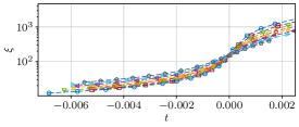
(a) $a=\infty$

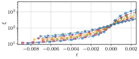
(b) $a=3.5$

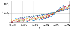
(c) $a=3.0$

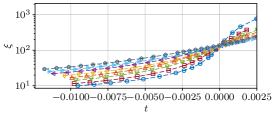
(d) $a=2.5$

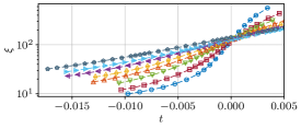
(e) $a=2.0$

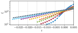
(f) $a=1.5$

(g)

Figure 1: (Colour online) Correlation length $[\xi(T)]$ as function of the reduced temperature $t$ for all considered correlation exponents $a$ and defect concentrations $p_{d}$. The definition (2.4) of $\xi$ is valid only in the high-temperature phase with $t\leqslant 0$, but we extended the curves in order to see the crossing points at $t\approx 0$ better.

3.1 Critical exponent $\nu$

By plotting the disorder averaged correlation length $[\xi(T)]$ for various defect concentrations $p_{d}$ as a function of $t$, we visually verified the used $T_{c}$ estimates (that depend on both $a$ and $p_{d}$), as can be seen in figure 1 where a negative reduced temperature $t\leqslant 0$ corresponds to the high-temperature phase. All the curves for different $p_{d}$ intersect at $t\approx 0$. Only for the strongest correlations with $a\leqslant 2.0$, visually not all of them intersect in one point. Strictly speaking, $\xi$ is defined only in the high-temperature phase where $t\leqslant 0$, but we extended it to $t>0$ in order to see the intersections better.

Considering only the high-temperature values with $t\leqslant 0$, we performed for each correlation exponent $a$ and each defect concentration $p_{d}$ an individual fit with the ansatz

$$\ln[\xi(t)]=A-\nu\ln|t|\,.$$ (3.1)

Since the power-law behaviour only starts at a certain distance away from $t=0$, i.e., once finite-size effects become neglectable, we varied the smallest $|t|_{\rm min}$ included in the fits from its smallest value near $t=0$ to a maximum value where only three degrees of freedom remained. Examples of the fits are presented in figure 2 which shows one main problem with this procedure. We clearly observe finite-size effects for each $p_{d}$, since the data points curve down as $|t|\to 0$. Compare, e.g., the plot for $a=1.5$ where this effect is most pronounced. However, since the statistical errors (estimated with the Jackknife method [28]) are quite large, linear fits still provide reasonable $\chi^{2}_{\rm red}$ values per degree of freedom. The resulting estimates of the exponent $\nu$ together with the $\chi^{2}_{\rm red}$ values for each $a$ and $p_{d}$ and for all the considered $|t|_{\rm min}$ are shown in figure 3. The data show a clear dependence on the defect concentration $p_{d}$ and also on $|t|_{\rm min}$. They do not reach the plateau value even for the largest $|t|_{\rm min}$ and the estimates for $p_{d}\leqslant 0.1$ are clearly influenced by the crossover to the pure Ising model. This reflects the observation in figure 1 that $[\xi]$ exhibits the strongest curvature for the smallest defect concentration $p_{d}$. Therefore, for a quantitative comparison, we computed the error weighted mean $\overline{\nu}_{\rm ts}^{w}$ over all estimates for $p_{d}\geqslant 0.15$ where for each $p_{d}$ we used the fit with the largest possible $|t|_{\rm min}$ having three degrees of freedom. This may be not an optimal solution but at least it was closer to possible plateau values than using the fits with the smallest possible $|t|_{\rm min}$ for which $\chi^{2}_{\rm red}\leqslant 1.0$ was satisfied for the first time. The latter results are way too low and clearly do not represent the asymptotic behaviour. As mentioned above, this is due to the relatively large statistical errors which made the simple linear fits acceptable, even though finite-size effects were still present.

The weighted means $\overline{\nu}_{\rm ts}^{w}$ are compared in the narrow right-hand panels of figure 3 with the estimates from our FSS analysis: Weighted means $\overline{\nu}^{w}_{\rm lin}$ of individual linear fits neglecting the scaling corrections [29] and $\nu^{\rm g}$ from non-linear “global” fits including corrections-to-scaling [29, 21, 30]. The numerical values are compiled in table 1 where we additionally include the weighted means $\overline{\nu}^{w}$ of non-linear FSS fits including the scaling corrections [29]. Except for $a=1.5$, the estimates $\overline{\nu}^{w}_{\text{ts}}$ obtained from temperature scaling are closer to $\overline{\nu}^{w}_{\rm lin}$ than to $\overline{\nu}^{w}$ respectively $\nu^{\rm g}$ and are slightly larger. The value for $a=1.5$ is possibly smaller because the estimates for larger $p_{d}$ show very large errors and hence the smallest included defect concentration $p_{d}=0.15$ dominates the weighted mean. Hence, the estimate for this value of $a$ should be considered with some reservation even though the exemplary fits for $a=1.5$ displayed in figure 2(f) do not look particularly worrying. The biggest deviations can be seen for the two correlation exponents $a=3.0$ and $3.5$ which is exactly the same behaviour as for the two types of FSS estimates, i.e., $\overline{\nu}^{w}_{\rm lin}$ and $\overline{\nu}^{w}$ or $\nu^{\rm g}$. We interpret this as a signal for the theoretically expected crossover from the correlated to effectively uncorrelated behaviour at $a\approx d=3$.

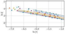
(a) $a=\infty$

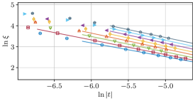
(b) $a=3.5$

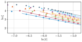
(c) $a=3.0$

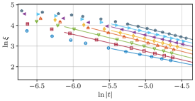
(d) $a=2.5$

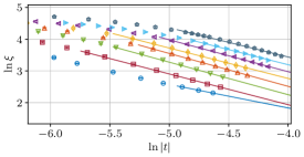
(e) $a=2.0$

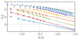
(f) $a=1.5$

(g)

Figure 2: (Colour online) Examples of the fits of $[\xi(t)]$ with the ansatz (3.1). For each concentration of defects $p_{d}$ the smallest $|t|_{\rm min}$ for which $\chi^{2}\leqslant 1.0$ was true for the first time is used in the plots.

Although one should take the estimates $\overline{\nu}^{w}_{\text{ts}}$ with some care, we nevertheless can qualitatively confirm the FSS results in all the considered cases. The prediction (1.1) of Weinrib and Halperin [15] that $\nu=2/a$ is not matched quantitatively. The results lie above this prediction, but the dependence on $a$ respectively the measured $\overline{a}$ is clearly in accordance with the FSS results which indeed show a $\propto 1/\overline{a}$ behaviour [21]. For a comparison with previous results for selected cases of $a$ and $p_{d}$ by other groups [31, 32, 33, 34, 35], we refer to table I and to the discussion in [20, 21]. Let us finally note that we also have checked the influence of the statistical error of the $T_{c}$ estimates on the results, but it turned out that it can be neglected due to much larger errors coming from the fits themselves.

3.2 Critical exponent $\gamma$

For the fits of the susceptibility $[\tilde{\chi}(T)]$ in the high-temperature phase, we used the ansatz

$$\ln[\tilde{\chi}(t)]=B-\gamma\ln|t|$$ (3.2)

and again performed individual fits for all correlation exponents $a$ and defect concentrations $p_{d}$. As in the case of $\xi(T)$, we varied the minimal $|t|_{\rm min}$ included in the fits to see the asymptotic behaviour.

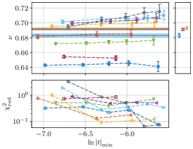
(a) $a=\infty$

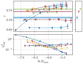
(b) $a=3.5$

(c) $a=3.0$

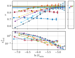
(d) $a=2.5$

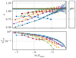
(e) $a=2.0$

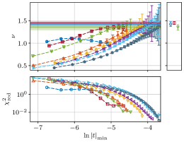
(f) $a=1.5$

(g)

Figure 3: (Colour online) Final fit results of $[\xi(t)]$ using the ansatz (3.1) for different $|t|_{\rm min}$ and all concentrations of defects $p_{d}$. The weighted means $\overline{\nu}^{w}_{\text{ts}}$ over all concentrations with $p_{d}\geqslant 0.15$ and for the largest possible $|t|_{\rm min}$ are shown together with the results $\overline{\nu}^{w}_{\rm lin}$ and $\nu^{\rm g}$ from the FSS analysis [21, 29]. The narrow right-hand panels show a separate comparison between the different estimates for $\nu$ which are plotted as horizontal lines in the main plots.

The susceptibility as function of $t$ is presented in figure 4. It has the same qualitative behaviour as $\xi$—for different $p_{d}$ the curves cross each other at $t\approx 0$. Note that as in the case of $\xi$, the definition of $\tilde{\chi}$ is valid only in the high-temperature phase, and we only extended the $T$ values below $T_{c}$ in order to see the crossing points better. In figure 5 we show examples of the fits for all correlation exponents $a$ and defect concentrations $p_{d}$. The estimates of the critical exponent $\gamma$ in dependence on the chosen $|t|_{\rm min}$ are presented in figure 6. The error weighted means of $\gamma$ over all $p_{d}\geqslant 0.15$ with the largest $|t|_{\rm min}$ are summarized in table 1.

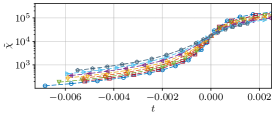
(a) $a=\infty$

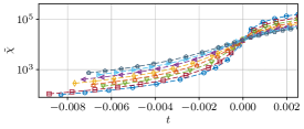
(b) $a=3.5$

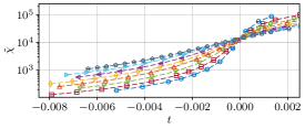
(c) $a=3.0$

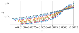
(d) $a=2.5$

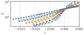
(e) $a=2.0$

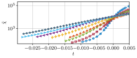
(f) $a=1.5$

(g)

Figure 4: (Colour online) Susceptibility $[\tilde{\chi}(T)]$ as function of the reduced temperature $t$. The definition of $\tilde{\chi}$ is valid only in the high-temperature phase with $t\leqslant 0$, but we extended the curves in order to see the crossing points better.

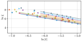
(a) $a=\infty$

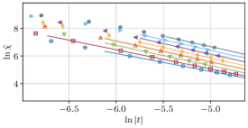
(b) $a=3.5$

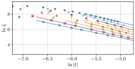
(c) $a=3.0$

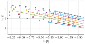
(d) $a=2.5$

(e) $a=2.0$

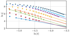
(f) $a=1.5$

(g)

Figure 5: (Colour online) Examples of the fits of $[\tilde{\chi}(t)]$ with the ansatz (3.2). For each concentration of defects $p_{d}$ the minimum $|t|_{\rm min}$ for which $\chi^{2}\leq 1.0$ was true for the first time is used in the plots.

The first observation is the same as in the case of $\xi$: The smallest concentrations $p_{d}\leqslant 0.1$ show a crossover behaviour and therefore we excluded them in the weighted mean. Again, the curves do not reach the asymptotic values even for the largest $|t|_{\rm min}$. The final weighted mean estimates $\overline{\gamma}^{w}_{\text{ts}}$ lie slightly above the corrected global fit estimates $\gamma^{\rm g}$ from the FSS analysis except for the case of $a=1.5$. They match very well for the correlation exponents in the range $2.0\leqslant a\leqslant 3.0$ but do not agree well in the uncorrelated case, $a=\infty$. The crossover region with $a\approx 3.0-3.5$ shows the largest deviations between $\overline{\gamma}^{w}_{\text{ts}}$ and $\gamma^{\rm g}$. In general, however, the qualitative cross-check with temperature scaling does support our estimates from the FSS analysis [21]. Unfortunately, here we cannot compare with the individual uncorrected fit ansatz in the FSS case, since we have not performed it for the critical exponent $\gamma$.

Table 1: Comparison of final estimates for the critical exponents $\nu$ and $\gamma$ from temperature-scaling (labeled with “ts”) and FSS analyses for several (input) correlation exponents $a$ together with their actual numerically measured values $\overline{a}$. The weighted means $\overline{\nu}^{w}_{\text{ts}}$ and $\overline{\gamma}^{w}_{\text{ts}}$ over $p_{d}\geq 0.15$ were calculated over the estimates with the maximal $|t|_{\rm min}$ (and hence three degrees of freedom). The FSS estimates $\nu^{\rm g}$ and $\gamma^{\rm g}$ are taken from [21] and $\overline{\nu}^{w}_{\rm lin}$ and $\overline{\nu}^{w}$ from [29].

$a$	$\overline{a}$	$\overline{\nu}^{w}_{\text{ts}}$	$\overline{\nu}^{w}_{\rm lin}$	$\overline{\nu}^{w}$	$\nu^{\rm g}$	$\overline{\gamma}^{w}_{\text{ts}}$	$\gamma^{\rm g}$
$\infty$	$\infty$	0.6928(17)	0.6913(15)	0.6843(31)	0.6831(30)	1.3430(18)	1.3324(64)
3.5	3.30(18)	0.7557(25)	0.7427(25)	0.7122(49)	0.7117(49)	1.4875(33)	1.451(15)
3.0	2.910(96)	0.7898(34)	0.7812(35)	0.7532(53)	0.7484(52)	1.5726(50)	1.566(16)
2.5	2.451(26)	0.8905(82)	0.8887(61)	0.8725(96)	0.8719(96)	1.787(11)	1.783(24)
2.0	1.979(18)	1.073(23)	1.079(14)	1.067(23)	1.060(23)	2.171(27)	2.149(51)
1.5	1.500(30)	1.348(61)	1.449(32)	1.435(56)	1.421(55)	2.791(70)	2.93(14)

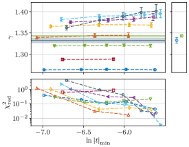
(a) $a=\infty$

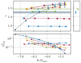
(b) $a=3.5$

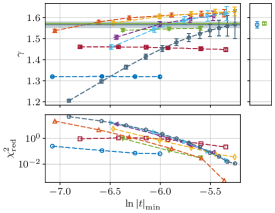
(c) $a=3.0$

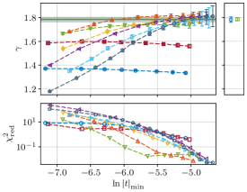
(d) $a=2.5$

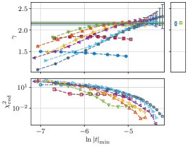
(e) $a=2.0$

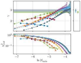
(f) $a=1.5$

(g)

Figure 6: (Colour online) Final results of the fits of $[\tilde{\chi}(t)]$ with the ansatz (3.2) for different $|t|_{\rm min}$ and all defect concentrations $p_{d}$. The weighted means $\overline{\gamma}^{w}_{\text{ts}}$ over all concentrations with $p_{d}\geqslant 0.15$ and for the largest possible $|t|_{\rm min}$ are shown together with the result from the FSS analysis $\gamma^{\rm g}$. The narrow right-hand panels show a separate comparison between the different estimates for $\gamma$ which are plotted as horizontal lines in the main plots.

4 Conclusions

The main merit of temperature scaling is its conceptual simplicity. It provides direct estimates of the critical exponents $\nu$, $\gamma$, …, whereas in the complementary FSS approach they can only be computed from the fitted exponent ratios $1/\nu$, $\gamma/\nu$, …which requires some care with statistical error propagation. A drawback of temperature scaling is that the determination of a suitable fit interval requires care at both ends. If the included temperatures $T$ are too far away from $T_{c}$, corrections-to-scaling cannot be neglected. At the other end, the included $T$ values should not be too close to $T_{c}$, because finite-size effects become important. By contrast, in the FSS approach, only the lower end of the fit interval needs to be controlled: The minimal lattice size $L$ must be large enough to avoid sizeable corrections-to-scaling. In this case, in FSS analyses one generically deals with simple linear two-parameter fits (since $T_{c}$ only enters indirectly), whereas in temperature scaling, this is only possible when $T_{c}$ is known from other sources (otherwise more cumbersome non-linear three-parameter fits are necessary). Of course, in both approaches, the situation becomes more complicated when corrections-to-scaling should be included since this introduces additional parameters and generically requires a non-linear many-parameter fitting.

Here, we successfully used the temperature-scaling analysis to validate our FSS results [21] for the critical exponents $\nu$ and $\gamma$. Considering that mostly different data entered the analysis and also different observables were used, i.e., the correlation length $\xi$ that was not studied in the FSS approach and the high-temperature definition of the susceptibility, we can clearly solidify our FSS results. Additionally, the critical temperatures estimated in the FSS study [21] were confirmed to be reasonably accurate to be used in the temperature-scaling analysis.

The available data turned out, however, to be not sufficiently accurate to perform fits including corrections-to-scaling, and the uncorrected fits show a clear dependence on the temperature range used. In order to improve the temperature-scaling analysis, we would need more simulated temperatures and also change the setup of the entire simulation process by using more disorder realizations instead of longer measurement time series for each realization, which is planned for future work.

Ukrainian 0

[Ñòåïåíåâà cêîðåëüîâàíà íåâïîðÿäêîâàíà 3D ìîäåëü Içiíãà]Àíàëiç òåìïåðàòóðíîãî ñêåéëiíãó òðèâèìiðíî¿ íåâïîðÿäêîâàíî¿ ìîäåëi Içiíãà çi ñòåïåíåâèìè ñêîðåëüîâàíèìè äåôåêòàìè Ñ. Êàçìií${}^{\textsf{\footnotesize{\mbox{?},\penalty 1000\mbox{?}}}}$, Â. ßíêå${}^{\textsf{\footnotesize{\mbox{?}}}}$

             
${}^{\textsf{\footnotesize 1}}$ Iíñòèòóò òåîðåòèчíî¿ ôiçèêè, Óíiâåðñèòåò Ëåéïöèãà, IPF 231101, 04801 Ëåéïöèã, Íiìåччèíà ${}^{\textsf{\footnotesize 2}}$ Íiìåöüêèé íåêîìåðöiéíèé íàóêîâî-äîñëiäíèé öåíòð áiîëîãiчíèõ ìàòåðiàëiâ, Òîðãàóåð øòð. 116, 04347 Ëåéïöèã, Íiìåччèíà

References

- [1] Harris A. B., J. Phys. C: Solid State Phys., 1974, 7, 1671–1692, doi:10.1088/0022-3719/7/9/009.
- [2] Ballesteros H. G., Fernández L. A., Martín-Mayor V., Muñoz Sudupe A., Parisi G., Ruiz-Lorenzo J. J., Phys. Rev. B, 1998, 58, 2740–2747, doi:10.1103/PhysRevB.58.2740.
- [3] Calabrese P., Martín-Mayor V., Pelissetto A., Vicari E., Phys. Rev. E, 2003, 68, 036136 (17 pages), doi:10.1103/PhysRevE.68.036136.
- [4] Berche P.-E., Chatelain C., Berche B., Janke W., Comput. Phys. Commun., 2002, 147, 427–430, doi:10.1016/S0010-4655(02)00319-3.
- [5] Berche P.-E., Chatelain C., Berche B., Janke W., Monte Carlo Studies of Three-Dimensional Bond-Diluted Ferromagnets, In: High Performance Computing in Science and Engineering, Munich 2002, Wagner S., Hanke W., Bode A., Durst F. (Eds.), Springer, Berlin, 2003, 227–238, Preprint arXiv:cond-mat/0212504.
- [6] Janke W., Berche P.-E., Chatelain C., Berche B., Phase Transitions in Disordered Ferromagnets, In: NIC Symposium 2004, Proceedings, Wolf D., Münster G., Kremer M. (Eds.), John von Neumann Institute for Computing, Jülich, NIC Series, 2003, Vol. 20, 241–250.
- [7] Janke W., Berche P.-E., Chatelain C., Berche B., Quenched Disorder Distributions in Three-Dimensional Diluted Ferromagnets, In: Computer Simulation Studies in Condensed-Matter Physics XVI, Landau D. P., Lewis S. P., Schüttler H.-B. (Eds.), Springer, Berlin, 2004, 89–94, Preprint arXiv:cond-mat/0304642.
-
[8]
Berche P.-E., Chatelain C., Berche B., Janke W.,
Eur. Phys. J. B, 2004, 38, 463–474,
doi:10.1140/epjb/e2004-00141-x. - [9] Berche B., Berche P.-E., Chatelain C., Janke W., Condens. Matter Phys., 2005, 8, 47–58, doi:10.5488/CMP.8.1.47.
-
[10]
Janke W., Berche B., Chatelain C., Berche P.-E., Hellmund M.,
PoS, 2005, LAT2005, 018 (22 pages),
doi:10.22323/1.020.0018. -
[11]
Murtazaev A. K., Kamilov I. K., Babaev A. B.,
J. Exp. Theor. Phys., 2004, 99, 1201–1206,
doi:10.1134/1.1854807. - [12] Hasenbusch M., Toldin F. P., Pelissetto A., Vicari E., J. Stat. Mech., 2007, 2007, No. 02, P02016 (43 pages), doi:10.1088/1742-5468/2007/02/P02016.
- [13] Kos F., Poland D., Simmons-Duffin D., Vichi A., J. High Energ. Phys., 2016, 2016, No. 8, 36 (15 pages), doi:10.1007/JHEP08(2016)036.
-
[14]
Ferrenberg A. M., Xu J., Landau D. P.,
Phys. Rev. E, 2018, 97, 043301 (12 pages),
doi:10.1103/PhysRevE.97.043301. - [15] Weinrib A., Halperin B. I., Phys. Rev. B, 1983, 27, 413–427, doi:10.1103/PhysRevB.27.413.
- [16] Honkonen J., Nalimov M. Y., J. Phys. A: Math. Gen., 1989, 22, 751–763, doi:10.1088/0305-4470/22/6/024.
-
[17]
Korzhenevskii A. L., Luzhkov A. A., Schirmacher W.,
Phys. Rev. B, 1994, 50, 3661–3666,
doi:10.1103/PhysRevB.50.3661. -
[18]
Korzhenevskii A. L., Luzhkov A. A., Heuer H.-O.,
Europhys. Lett., 1995, 32, 19–24,
doi:10.1209/0295-5075/32/1/004. - [19] Dudka M., Fedorenko A. A., Blavatska V., Holovatch, Yu., Phys. Rev. B, 2016, 93, 224422 (13 pages), doi:10.1103/PhysRevB.93.224422.
- [20] Kazmin S., Janke W., Phys. Rev. B, 2020, 102, 174206 (13 pages), doi:10.1103/PhysRevB.102.174206.
- [21] Kazmin S., Janke W., Phys. Rev. B, 2022, 105, 214111 (12 pages), doi:10.1103/PhysRevB.105.214111.
- [22] Makse H., Havlin S., Stanley H. E., Schwartz M., Chaos, Solitons & Fractals, 1995, 6, 295–303, doi:10.1016/0960-0779(95)80035-F.
-
[23]
Makse H. A., Havlin S., Schwartz M., Stanley H. E.,
Phys. Rev. E, 1996, 53, 5445–5449,
doi:10.1103/PhysRevE.53.5445. -
[24]
Zierenberg J., Fricke N., Marenz M., Spitzner F. P., Blavatska V., Janke W.,
Phys. Rev. E, 2017, 96,
062125 (11 pages), doi:10.1103/PhysRevE.96.062125. - [25] Fricke N., Zierenberg J., Marenz M., Spitzner F. P., Blavatska V., Janke W., Condens. Matter Phys., 2017, 20, 13004 (11 pages), doi:10.5488/CMP.20.13004.
- [26] Swendsen R. H., Wang J.-S., Phys. Rev. Lett., 1987, 58, 86–88, doi:10.1103/PhysRevLett.58.86.
- [27] Janke W., In: Computational Many-Particle Physics, Lecture Notes in Physics, Vol. 739, Fehske H., Schneider R., Weiße A. (Eds.), Springer, Berlin Heidelberg, 2008, 79–140, doi:10.1007/978-3-540-74686-7_4.
- [28] Efron B., Tibshirani R., An Introduction to the Bootstrap, Monographs on Statistics and Applied Probability, Chapman & Hall, New York, 1993.
-
[29]
Kazmin S.,
Ising Model in Three Dimensions with Long-Range Power-Law Correlated Site
Disorder: A Monte Carlo Study,
PhD Thesis, Universität Leipzig, May 2021,
URL https://nbn-resolving.org/urn:nbn:de:bsz:15-qucosa2-798018. -
[30]
Blavats’ka V., von Ferber C., Holovatch Y.,
Phys. Rev. E, 2001, 64, 041102 (10 pages),
doi:10.1103/PhysRevE.64.041102. - [31] Ballesteros H. G., Parisi G., Phys. Rev. B, 1999, 60, 12912–12917, doi:10.1103/PhysRevB.60.12912.
-
[32]
Prudnikov V. V., Prudnikov P. V., Fedorenko A. A.,
Phys. Rev. B, 2000, 62, 8777–8786,
doi:10.1103/PhysRevB.62.8777. - [33] Prudnikov V. V., Prudnikov P. V., Dorofeev S. V., Kolesnikov V. Y., Condens. Matter Phys., 2005, 8, 213–224, doi:10.5488/CMP.8.1.213.
-
[34]
Ivaneyko D., Berche B., Holovatch Yu., Ilnytskyi J.,
Physica A, 2008, 387, 4497–4512,
doi:10.1016/j.physa.2008.03.034. -
[35]
Wang W., Meier H., Lidmar J., Wallin M.,
Phys. Rev. B, 2019, 100, 144204 (8 pages),
doi:10.1103/PhysRevB.100.144204.
Ukrainian \adddialect\l@ukrainian0 \l@ukrainian