Constraining parameters for the accelerating models in symmetric teleparallel gravity

Abstract

Abstract: Using the cosmological data sets, accelerating cosmological models are obtained in this paper by constraining the free parameters in symmetric teleparallel gravity. Using the best-fit values of free parameters, we determine the present values of geometrical parameters and the late-time behaviour of the universe. We also consider two $f(Q)$ models ($Q$ being the non-metricity scalar): one that contains the term of higher power of non-metricity scalar and the other with the inverse. From the constrained free parameters, the present values of the geometrical parameters are obtained and that of the effective equation of state parameter for both models. Interestingly, we found that all the values lie within the range prescribed by the cosmological observations. Further, the models exhibit the $\Lambda{CDM}$ behaviour at the late time of the evolution.
Keywords: Non-metricity scalar, Late time acceleration, Dark energy, Cosmological observation.

I Introduction

The theory of General Relativity (GR) is the most successful theory based on which plenty of cosmological models were proposed in the literature. Each model should be able to describe the observed accelerated expansion of the Universe [1, 2]. In GR, the accelerated expansion was assumed to be due to an exotic form of energy known as Dark Energy (DE). This behavior has been strongly supported with high precision observational pieces of evidence such as the Wilkinson Microwave Anisotropy Probe experiment (WMAP) [3], Baryonic Acoustic Oscillations (BAO) [4], Large Scale Structure (LSS) [5], Cosmic Microwave Background Radiation (CMBR) [6, 7], Baryon Oscillation Spectroscopic Survey (BOSS) [8], and the Planck collaboration [9, 10]. However, the DE models based on GR still face theoretical and observational problems.

In literature, one may find various modified theories of gravity beyond GR aiming to alleviate the problems. In the literature, there are two equivalent geometrical theories of GR based on the torsion and non-metricity, respectively known as the teleparallel equivalent of GR [11] and the symmetric teleparallel equivalent of GR [12]. Even if these two theories are equivalent to the GR, their corresponding extensions are not fundamentally equivalent [13]. In the present work, we shall consider the symmetric teleparallel equivalent of GR, which was further developed into the $f(Q)$ gravity theory or the coincident GR [14].

Recently, the $f(Q)$ theory of gravity was found to produce interesting cosmological phenomenology at the background and perturbation levels [15, 16, 17, 18, 21, 20, 19, 22, 23, 24]. The theory has also been successfully confronted with various observational data sets coming from the CMBR, SNIa, BAO, redshift space distortion, etc [25, 26, 27, 28, 29]. Anagnostopoulos et al. [30] showed that $f(Q)$ gravity can safely pass the Big Bang Nucleosynthesis constraints. The behavior of the dynamical parameters of $f(Q)$ gravity constrained by the scale factor and model parameters was studied in Refs. [31, 32, 33]). Maurya et al. [34] investigated the gravitationally decoupled anisotropic solutions for the strange stars in the framework of gravity by utilizing the CGD technique. Further, a class of $f(Q)$ theories were proposed, in which, the non-metricity $Q$ is non-minimally coupled to the matter Lagrangian [35] or to the scalar field [36] leading to interesting phenomenology. The reconstruction of the function $f(Q)$ through a numerical inversion procedure based on the current observational bounds of cosmographic parameters was performed in Ref. [37].

The $f(Q)$ gravity belongs to the symmetric teleparallel gravity, which is another modified gravity that attributes to the non-metricity. When the perturbation is considered around FLRW background, this gravity does not provide any strong coupling issue. So, the objective is to explore the impact of this gravity on the cosmological observations i.e. one can use the expansion rate data from the cosmological observations and constraint the parameters involved for different parametrization of the function in the redshift function [14, 38, 35, 39, 40, 16]. It might be possible that the phenomenological analysis of the non-metricity based gravity models may deviate from the cosmological observations. This may further provide an avenue to distinguish models from the $\Lambda$CDM scenario, and the interest remains with the constraining of model parameters. Further, to comply with the theoretical model with the late-time cosmic acceleration issue, the parameters need to be constrained with the data set available from the cosmological observations. At the respective discussion, the obtained result and the corresponding observational outcomes must be compared to validate the models.

The paper is organized as: Sec. II gives the basic mathematical formalism of $f(Q)$ gravity and the derivation of gravitational field equations are shown in Sec. III. In Sec. IV, the geometrical parameters are shown and several cosmological constraints are given in Sec. V. The models of $f(Q)$ gravity are discussed in Sec. VI. A summary of concluding remarks is provided in the Sec. VII.

II $f(Q)$ Gravity

In differential geometry, a general connection $\Sigma_{\mu\nu}^{\alpha}$ allows us to carry out parallel vector transport as well as to compute covariant derivatives, while metric tensor $g_{\mu\nu}$ provides us with information regarding angles, volumes, distances, etc. The latter can be thought of as a generalization of the so-called gravitational potential of classical theory. Generally, the connection $\Sigma_{\mu\nu}^{\alpha}$ can be decomposed into the following contributions (containing the torsion $T$, non-metricity $Q$ and the curvature term $R$) [41] as,

$$\Sigma_{\ \mu\nu}^{\alpha}=\Gamma_{\ \mu\nu}^{\alpha}+K_{\ \mu\nu}^{\alpha}+L_{\ \mu\nu}^{\alpha},$$ (1)

with the famous Levi-Civita connection $\Gamma_{\ \mu\nu}^{\alpha}$ corresponds the metric tensor $g_{\mu\nu}$ is,

$$\Gamma_{\ \mu\nu}^{\alpha}\equiv\frac{1}{2}g^{\alpha\lambda}(g_{\mu\lambda,\nu}+g_{\lambda\nu,\mu}-g_{\mu\nu,\lambda}),$$ (2)

and the Disformation tensor $L_{\ \mu\nu}^{\alpha}$ is given as,

$$L_{\ \mu\nu}^{\alpha}\equiv\frac{1}{2}(Q_{~{}~{}\mu\nu}^{\alpha}-Q_{\mu~{}~{}\nu}^{\ \alpha}-Q_{\nu~{}~{}\mu}^{\ \alpha})=L_{\ \nu\mu}^{\alpha}.$$ (3)

Finally, the expression for the Contortion tensor $K_{\ \mu\nu}^{\alpha}$ is,

$$K_{\ \mu\nu}^{\alpha}\equiv\frac{1}{2}(T_{~{}~{}\mu\nu}^{\alpha}+T_{\mu~{}~{}\nu}^{~{}\alpha}+T_{\nu~{}~{}\mu}^{~{}\alpha})=-K_{\ \nu\mu}^{\alpha}.$$ (4)

The quantities $Q_{\alpha\mu\nu}$ and $T_{\ \mu\nu}^{\alpha}$ in Eqs. (3) and (4), are the non-metricity tensor and the torsion tensor, respectively, which are given by

$$Q_{\alpha\mu\nu}\equiv\nabla_{\alpha}g_{\mu\nu}\neq 0,$$ (5)

$$T_{\ \mu\nu}^{\alpha}\equiv\Sigma_{\ \mu\nu}^{\alpha}-\Sigma_{\ \nu\mu}^{\alpha}.$$ (6)

It was shown in [14], that the connection presumed to be torsion and curvature vanish within the so-called Symmetric Teleparallel Equivalent to General Relativity (STEGR). The components of the connection in Eq. (1) can be rewritten as,

$$\Sigma^{\alpha}\,_{\mu\beta}=\frac{\partial y^{\alpha}}{\partial\xi^{\rho}}\partial_{\mu}\partial_{\beta}\xi^{\rho}.$$ (7)

In the above equation, $\xi^{\alpha}=\xi^{\alpha}(y^{\mu})$ is an invertible relation and $\frac{\partial y^{\alpha}}{\partial\xi^{\rho}}$ is the inverse of the corresponding Jacobian [17]. This situation is called a coincident gauge, where there is always a possibility of getting a coordinate system with connections $\Sigma_{\ \mu\nu}^{\alpha}$ equaling zero. Hence, in this choice, the covariant derivative $\nabla_{\alpha}$ reduces to the partial derivative $\partial_{\alpha}$ i.e. $Q_{\alpha\mu\nu}=\partial_{\alpha}g_{\mu\nu}$. Thus, it is clear that the Levi-Civita connection $\Gamma_{\ \mu\nu}^{\alpha}$ can be written in terms of the disformation tensor $L_{\ \mu\nu}^{\alpha}$ as $\Gamma_{\ \mu\nu}^{\alpha}=-L_{\ \mu\nu}^{\alpha}$.

The action that conforms with STEGR is described by,

$$S_{STEGR}=\int{\frac{1}{2}}\left({Q}\right){\sqrt{-g}d^{4}x}+\int{\mathcal{L}_{m}\sqrt{-g}d^{4}x},$$ (8)

where $g$ being the determinant of the tensor metric $g_{\mu\nu}$ and $\mathcal{L}_{m}$ the matter Lagrangian density. The modified $f(R)$ gravity is a generalization of GR, and the $f(T)$ gravity is a generalization of TEGR. Thus, in the same way, the $f(Q)$ is a generalization of STEGR in which the extended action is given by,

$$S=\int{\frac{1}{2}f(Q)\sqrt{-g}d^{4}x}+\int{\mathcal{L}_{m}\sqrt{-g}d^{4}x.}$$ (9)

Here $f(Q)$ is an arbitrary function of the non-metricity scalar $Q$, with $f\left(Q\right)=Q$ corresponds to the STEGR [14]. In addition, the non-metricity tensor in Eq. (5) has the following two independent traces,

$$Q_{\alpha}=Q_{\alpha}{}^{\mu}{}_{\mu}\text{ \ \ and \ \ }\tilde{Q}_{\alpha}=Q^{\mu}{}_{\alpha\mu}.$$ (10)

Further, the non-metricity conjugate known as superpotential tensor is given by,

$$P^{\lambda}_{~{}~{}\mu\nu}\equiv-\frac{1}{4}Q^{\lambda}_{~{}~{}\mu\nu}+\frac{1}{4}\left(Q^{~{}~{}\lambda}_{\mu~{}~{}\nu}+Q^{~{}~{}\lambda}_{\nu~{}~{}\mu}\right)+\frac{1}{4}Q^{\lambda}g_{\mu\nu}-\frac{1}{8}\left(2\tilde{Q}^{\lambda}g_{\mu\nu}+{\delta^{\lambda}_{\mu}Q_{\nu}+\delta^{\lambda}_{\nu}Q_{\mu}}\right).$$ (11)

The non-metricity scalar can be acquired as,

$$Q=-Q_{\lambda\mu\nu}P^{\lambda\mu\nu}.$$ (12)

Now, the energy-momentum tensor of the content of the Universe as a perfect fluid matter is given as,

$$T_{\mu\nu}=\frac{-2}{\sqrt{-g}}\frac{\delta(\sqrt{-g}\mathcal{L}_{m})}{\delta g^{\mu\nu}}.$$ (13)

By varying the above action (9) with regard to the metric tensor $g_{\mu\nu}$ components yield

$$\frac{2}{\sqrt{-g}}\nabla_{\lambda}(\sqrt{-g}f_{Q}P^{\lambda}\>_{\mu\nu})+\frac{1}{2}g_{\mu\nu}f+f_{Q}(P_{\mu\lambda\beta}Q_{\nu}\>^{\lambda\beta}-2Q_{\lambda\beta\mu}P^{\lambda\beta}\>_{\nu})=-T_{\mu\nu}.$$ (14)

Here, for simplicity we consider $f_{Q}=\frac{df}{dQ}$ . Again, by varying the action with regard to the connection, we can get as a result,

$$\nabla_{\mu}\nabla_{\nu}(\sqrt{-g}f_{Q}P^{\mu\nu}\mathrel{\mathop{\ordinarycolon}}_{\lambda})=0.$$ (15)

In the next section, we shall present the cosmological equations of the $f(Q)$ gravity within the context of the FLRW space-time.

III FLRW Universe in $f(Q)$ cosmology

The CMB indicates that our Universe is homogeneous and isotropic on a large scale, i.e. a scale greater than that of galaxy clusters. For this, in our current analysis, we consider a flat FLRW background geometry in Cartesian coordinates with a metric,

$$ds^{2}=-dt^{2}+a^{2}(t)[dx^{2}+dy^{2}+dz^{2}],$$ (16)

where $a(t)$ is the scale factor of the Universe, $t$ is the cosmic time and $x,y,z$ are Cartesian coordinates. Furthermore, the non-metricity scalar corresponding to the metric (16) is obtained as $Q=6H^{2}$, where $H=\frac{\dot{a}}{a}$ is the Hubble parameter that measures the rate of expansion of the Universe. In cosmology, the most commonly used matter component is the perfect cosmic fluid whose energy-momentum tensor ( without considering viscosity effects) is

$$T_{\mu\nu}=(\rho+p)u_{\mu}u_{\nu}+pg_{\mu\nu}.$$ (17)

Here, $\rho$ and $p$ represent the cosmic energy density and isotropic pressure of the perfect cosmic fluid, respectively, and $u^{\mu}=(1,0,0,0)$ represents the four-velocity vector components characterizing the fluid.

The modified Friedmann equations that describe the dynamics of the Universe in $f(Q)$ gravity are [35, 16],

$$3H^{2} = \frac{1}{2f_{Q}}\left(\rho+\frac{f}{2}\right),$$ (18)

$$\dot{H}+3H^{2}+\frac{\dot{f}_{Q}}{f_{Q}}H = \frac{1}{2f_{Q}}\left(-p+\frac{f}{2}\right),$$ (19)

here an overhead dot points out the differentiation of the quantity with regard to cosmic time $t$. Also, it is worth noting that the standard Friedmann equations of GR are obtained if the function $f(Q)=Q$ is assumed [16].

In this work, we consider that the matter component composed of the pressureless matter and radiation whose conservation equation can be respectively written as,

$$\dot{\rho}_{m}+3H\rho_{m}=0,~{}~{}~{}~{}~{}~{}~{}~{}~{}~{}~{}~{}~{}~{}~{}~{}~{}~{}~{}~{}~{}~{}\dot{\rho}_{r}+4H\rho_{r}=0,$$ (20)

which gives us $\rho_{m}\propto a^{-3}$ and $\rho_{r}\propto a^{-4}$. Here, $\rho_{m},\rho_{r}$ denotes the energy density components of pressureless matter and radiation, respectively. Using the form $f(Q)=Q+F(Q)$ in Eqs. (18) and (19), one may also the express the effective energy density $\rho_{\rm eff}$ and effective pressure $p_{eff}$ of the fluid in terms of geometrical terms as [22],

$$\rho_{\rm eff} = \rho_{m}+\rho_{r}+\underbrace{\frac{F-2QF_{Q}}{2}}_{\rho_{de}},$$ (21)

$$p_{\rm eff} = p_{m}+p_{r}+\underbrace{QF_{Q}+2\dot{H}(2QF_{QQ}+F_{Q})-\frac{F}{2}}_{p_{de}}.$$ (22)

Note that $\rho=\rho_{m}+\rho_{r}$ and $p=p_{m}+p_{r}$. Further, with the help of Eqs. (21) and (22), one may also introduce the equation of state (EoS) for dark energy and a quantity which determines the acceleration expansion of the Universe known as the effective EoS given by,

$$\omega_{de} = \frac{p_{de}}{\rho_{de}}=-1+\frac{4\dot{H}(2QF_{QQ}+F_{Q})}{F-2QF_{Q}},$$

$$\omega_{\rm eff} = \frac{p_{\rm eff}}{\rho_{\rm eff}}=\frac{-F+4\dot{H}(F_{Q}+2QF_{QQ})+2(QF_{Q}+p_{m}+p_{r})}{F-2QF_{Q}+2\rho_{m}+2\rho_{r}}.$$ (23)

We say that the model is a cosmological constant ($\Lambda CDM$) whenever $\omega_{\rm eff}=-1$, a quintessence model when $-1<\omega_{\rm eff}\leq-\frac{1}{3}$, and a phantom model whenever $\omega_{\rm eff}<-1$. The numerical value of the EoS parameter has also been constrained by several cosmological analyses, such as Supernovae Cosmology Project, $\omega_{\rm eff}=-1.035_{-0.059}^{+0.055}$ [42]; WAMP+CMB, $\omega_{\rm eff}=-1.079_{-0.089}^{+0.090}$ [7]; Plank 2018, $\omega_{\rm eff}=-1.03\pm 0.03$ [10].

IV Cosmographic Parameters

In this section, we shall introduce some cosmographic parameters such as the deceleration parameter $q$ and state finder parameters $\{j,s\}$, where $j$ and $s$ respectively, known as the jerk and snap parameters. To distinguish the dark energy models, these parameters will be of utmost useful. The cosmographic parameters are geometrical quantities, which can be obtained from the scale factor and, thereby, from the metric potentials. Using several cosmological data sets, one can find the present values of these parameters. We consider the parametrization of the Hubble parameter as [43],

$$H=\frac{H_{0}}{\epsilon+1}\left(a^{-\gamma}+\epsilon\right)\,,$$ (24)

To ensure the positivity of the Hubble parameter and the expansion of the Universe realised, in Eq. (24), $\frac{H_{0}}{\epsilon+1}>0$ and the signature of $\gamma$ will not have any effect on its expanding behaviour. For $\epsilon=1$, we can obtain $H(z)=\eta\left(1+(1+z)^{-\gamma}\right)$ [33] and we consider $\epsilon>-1$ to avoid the singularity as well as to maintain positiveness of $H(z)$. Using the scale factor and redshift relation, $a=\frac{1}{1+z}$, Eq. (24) becomes

$$H(z)=\xi\left(\epsilon+(1+z)^{\gamma}\right),~{}~{}~{}~{}~{}~{}~{}~{}~{}~{}~{}\left(\xi=\frac{H_{0}}{\epsilon+1}\right).$$ (25)

The deceleration parameter $q(z)$ can be defined as,

$$q(z)=-1+\frac{(1+z)}{H(z)}\frac{dH(z)}{dz}.$$ (26)

Eq. (26) provides the decelerating or accelerating behaviour of the Universe. The positive value of $q$ refers to a decelerating phase of the Universe, whereas the negative value corresponds to the accelerating phase. Some cosmological observations revealed its present value as: $q_{0}=-0.51^{+0.09}_{-0.01}$ , $q_{0}=-0.5422_{-0.0826}^{+0.0718}$ and a transition redshift from deceleration to acceleration is $z_{t}=0.65^{+0.19}_{-0.17}$ , $z_{t}=0.8596_{-0.2722}^{+2886}$ [44, 46, 45]. Further, the statefinder pair can be defined as,

$$j(z) = q(z)+2q^{2}(z)+(1+z)\frac{dq(z)}{dz},$$ (27)

$$s(z) = \frac{j(z)-1}{3\left(q(z)-\frac{1}{2}\right)},~{}~{}~{}~{}~{}~{}~{}~{}~{}~{}~{}~{}~{}~{}\left(q\neq\frac{1}{2}\right).$$ (28)

Based on the values of these parameters, Sahni et al [47, 48] provides the followings: (i)$(j=1,~{}s=0)\rightarrow\Lambda CDM$; (ii) $(j<1,~{}s>0)$$\rightarrow$ Quintessence; (iii) $(j>1,~{}s<0)\rightarrow$ Chaplygin Gas; and (iv) $(j=1,~{}s=1)\rightarrow$SCDM. It is noteworthy to mention that, $\left\{j,~{}s\right\}=\left\{1,0\right\}$ represents the point corresponding to the flat $\Lambda$CDM model. Keeping this as a reference point, one can find the departure of the models from flat $\Lambda$CDM. Further in the $\left\{j,~{}s\right\}$ plane, $s>0$ and $s<0$ respectively indicate the quintessence-like and the Phantom-like dark energy models. Also, when $\left\{j,~{}s\right\}$ passes through a point $\left\{1,0\right\}$ in the $j-s$ plane, the evolution from phantom to quintessence can be obtained. So, one can classify the modified gravity, and dark energy cosmological models using the analysis of state finder pair [49].

V Observational constraints

In this section, we shall use the data sets from various cosmological observations to constrain the free parameters of $H(z)$ i.e. use of data that describes the distance-redshift relationship. We shall use the expansion rate data from early-type galaxies like $H(z)$ data, $Pantheon$ data, $Pantheon+Analysis$ data, $BAO$ (Baryon Acoustic Oscillations) data and the $CMB$ (Cosmic Microwave Background) distance priors. These observational data sets are independent of any given cosmological model and a tool to estimate the cosmological parameters. A brief discussion of each of these is given below:

V.1 Monte Carlo Markov Chain (MCMC)

The best-fit values of the free parameters are constrained by considering the $H(z)$, $Pantheon$ and $Pantheon+Analysis$ data sets with the MCMC process. To perform this, we use the Scipy optimization technique from the Python library together with the consideration of a Gaussian prior with a fixed $\sigma=1.0$ as the dispersion using the emcee package. The panels on the diagonal corner of the MCMC plot show the $1-D$ curve for each model parameter obtained by marginalizing over the other parameters, with a thick line curve to indicate the best-fit value. The off-diagonal panels show $2-D$ projections of the posterior probability distributions for each pair of parameters, with contours to indicate $1-\sigma$ and $2-\sigma$ regions. The main objective of this technique is to maximize the total likelihood function $\mathcal{L}_{\rm tot}\simeq e^{-\chi^{2}/2}$ which is equivalent to minimizing the total $\chi^{2}$. Here, $\chi^{2}$ is determined by the contributions obtained from the $Hubble$, $Pantheon$ and $Pantheon+Analysis$ data sets i.e. $\chi^{2}_{H(z)}$ and $\chi_{SN}^{2}$ respectively as

$$\chi^{2}=\chi^{2}_{H(z)}+\chi_{SN}^{2}\,.$$ (29)

In what follows, we briefly discuss the construction of $\chi^{2}$ from various data sets.

V.2 $H(z)$ data

A list of $32$ data points of the Hubble parameter is provided in Table 2 for the redshift range $0.07\leq z\leq 1.965$ [50]. By minimizing the Chi-square value, we determine the mean values of the model parameters $H_{0}$, $\epsilon$, and $\gamma$. The Chi-square function from the Hubble data is given as,

$$\chi_{H(z)}^{2}(p_{s})=\sum_{i=0}^{32}\frac{\left[H_{th}(z_{i},p_{s})-H_{obs}(z_{i})\right]^{2}}{\sigma_{H}^{2}(z_{i})},$$ (30)

where $H_{obs}(z_{i})$ represents the observed Hubble parameter values, $H_{th}(z_{i},p_{s})$ represents the Hubble parameter with the model parameters and $\sigma_{H}^{2}(z_{i})$ is the standard deviation.

V.3 $Pantheon+Analysis$ data

The $Pantheon+Analysis$ sample data set consists of 1701 light curves of 1550 distinct Type Ia supernovae ranging in redshift from $z=0.00122$ to $2.2613$ [51]. The model parameters are to be fitted by comparing the observed and theoretical values of the distance moduli. The $\chi^{2}_{SN}$ function from $Pantheon+Analysis$ sample of 1701 is given by,

$$\chi^{2}_{SN}(z,p_{s})=\sum_{i,j=0}^{1701}\nabla\mu_{i}\left(C_{SN}^{-1}\right)\nabla\mu_{j},$$ (31)

where $p_{s}$ represents the model parameters and $C_{SN}$ is covariance matrix [52]. Once a specific cosmological model has been chosen, the predicted distance modulus $\mu$ is defined as,

$$\mu(z,p_{s})=5\log_{10}[d_{L}(z,p_{s})]+\mu_{0},$$ (32)

where $\mu_{0}$ is the nuisance parameter and $d_{L}$ is the dimensionless luminosity distance defined as,

$$d_{L}(z)=(1+z)\int_{0}^{z}\frac{d\tilde{z}}{E(\tilde{z})},$$ (33)

with $E(z)=\frac{H(z)}{H_{0}}$ is the dimensionless parameter and $\tilde{z}$ is variable change to define integration from $0$ to $z$.

V.4 $BAO/CMB$ Constraints

We verify the obtained values of $H(z)$ parameters presented in TABLE-1 with the $BAO/CMB$ data. The $\chi^{2}$ for the BAO/CMB analysis using acoustic scale is given as

$$\chi_{\textit{BAO/CMB}}^{2}=X^{T}C^{-1}X,$$

where $X$ depends on the survey considered and the inverse of covariance matrix $C$ is given by [53], $X=\begin{pmatrix}\frac{d_{A}(z_{*})}{D_{V}(0.106)}-30.95\\ \frac{d_{A}(z_{*})}{D_{V}(0.200)}-17.55\\ \frac{d_{A}(z_{*})}{D_{V}(0.350)}-10.11\\ \frac{d_{A}(z_{*})}{D_{V}(0.440)}-8.44\\ \frac{d_{A}(z_{*})}{D_{V}(0.600)}-6.69\\ \frac{d_{A}(z_{*})}{D_{V}(0.730)}-5.45\end{pmatrix}$   and   $C^{-1}=\begin{pmatrix}0.48435&-0.101383&-0.164945&-0.0305703&-0.097874&-0.106738\\ -0.101383&3.2882&-2.45497&-0.0787898&-0.252254&-0.2751\\ -0.164945&-2.45497&9.55916&-0.128187&-0.410404&-0.447574\\ -0.0305703&-0.0787898&-0.128187&2.78728&-2.75632&1.16437\\ -0.097874&-0.252254&-0.410404&-2.75632&14.9245&-7.32441\\ 0.106738&-0.2751&-0.447574&1.16437&-7.32441&14.5022\\ \end{pmatrix}$ . The expression for the comoving angular-diameter distance [$d_{A}(z_{*})$] and the dilation scale [$D_{V}(z)$] are respectively,

$$d_{A}(z_{*}) = \int_{0}^{z_{*}}\frac{d\tilde{z}}{H(\tilde{z})},$$

$$D_{V}(z) = \left[\frac{(d_{A}(z))^{2}cz}{H(z)}\right]^{\frac{1}{3}}.$$ (34)

The epoch at which baryons were released from photons is called drag epoch $(z_{d})$. At this epoch, the photon pressure is no longer able to avoid the gravitational instability of the baryons. In the present work, we use the value, $z_{d}=1020$ [54].

The Results: After successfully implementing the MCMC process, we got the best fit and mean values of the cosmological free parameters $H_{0}$, $\epsilon$ and $\gamma$ that appear in Table 1. In FIG.- 1, we present the confidence contours along with the marginalized posterior distribution of different cosmological parameters from the $H(z)$ data set, $Pantheon+Analysis$ data set and combine $H(z)+Pantheon+Analysis$ data set. The constrained values obtained for the free parameters $H_{0}$, $\epsilon$ and $\gamma$ using these data sets are summarized in 1. FIG.- 2 shows the best-fit curves for the model described by (25) and for the standard $\Lambda$CDM with various data points. It can be noted that an exciting feature is perceived in the value of the Hubble constant defined as $H_{0}=100h$. With respect to the values acquired and the one forecast by Planck, our end result for $H_{0}$ perfectly resembles the value of Planck $\Lambda$CDM estimation [10]. We can observe that both the solid red line and the broken black line appear inside the error bars.

Data sets	H(z)	Pantheon+Analysis	H(z)+Pantheon+Analysis
$H_{0}$	$68.47\pm 0.6$	$69\pm 0.63$	$68.9_{-1.7}^{+1.8}$
$\epsilon$	$2.63\pm 0.74$	$3.92\pm 0.90$	$4.0^{+1.1}_{-1.0}$
$\gamma$	$1.9\pm 0.16$	$2.19\pm 0.19$	$2.28^{+0.27}_{-0.25}$
$q_{0}$	$-0.476584$	$-0.554878$	$-0.544$
$j_{0}$	$0.698207$	$0.837585$	$0.879616$

Table 1: Best fit mean values of the free cosmological parameters and present value of deceleration and jerk parameter.

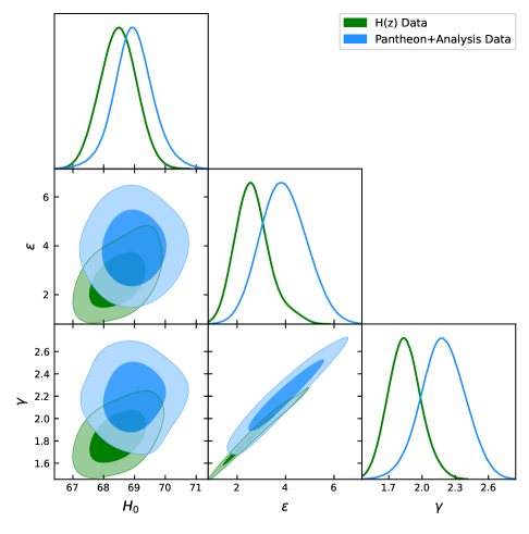
Figure 1: MCMC 1$\sigma$ and 2$\sigma$ confidence contour plot obtained from $H(z)$ data set and $Pantheon+Analysis$ data set (Left panel) and combine $H(z)+Pantheon+Analysis$ data set (Right panel).

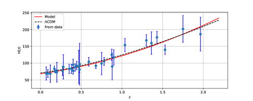
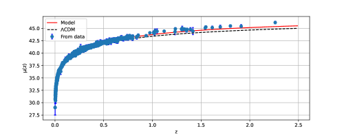
Figure 2: $H(z)$ in redshift from 32 data points of $H(z)$ data (Upper panel). $\mu(z)$ in redshift in $Pantheon+Analysis$ data set (Lower panel). Blue error bars from the data set, red solid line for the model and broken black line for $\Lambda$ CDM.

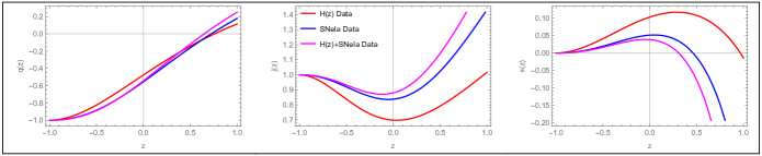
Figure 3: Deceleration parameter (Left panel), jerk parameter (Middle panel), snap parameter(Right panel)

.

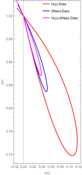
Figure 4: The State finder pair $(j,~{}s)$ is shown for different data sets

.

Once we obtained the range of the free parameters, we can further examine the behaviour of other geometrical parameters. From FIG.- 3, we can observe that $q(z)$ shows the transition from deceleration to acceleration. The transition point for $H(z)$ data set, $Pantheon+Analysis$ data set and combine $H(z)+Pantheon+Analysis$ data set is $z_{t}=0.75$, $z_{t}=0.72$ and $z_{t}=0.65$ respectively. The present value of the deceleration parameter for each data set has been summarized in Table 1. Also the $(j,~{}s)$ values for $H(z)$ data set, $Pantheon+Analysis$ data set and combine $H(z)+Pantheon+Analysis$ data set are $(0.7,0.1)$, $(0.83,0.05)$ and $(0.88,0.03)$ respectively. From $(j,~{}s)$ value, one can infer the quintessence behavior of the model at present time FIG.- 4.

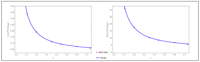
Figure 5: $\frac{r_{s}(z_{d})}{D_{V}(z_{BAO})}$ parameter (Left Panel) and BAO/CMB constraints (Right panel) in redshift.

Further, We have checked the compatibility of our results with the new measurement of $\frac{r_{s}(z_{d})}{D_{V}(z)}$ [Percival et al. [55]] at $z=0.2$ and $z=0.35$, the 6dF Galaxy Survey at $z=0.106$ [56] and the WiggleZ team [57] at $z=0.44$, $z=0.60$ and $z=0.73$ in FIG.-5 [Left panel]. We have used the obtained best-fit values of model parameters to plot the $BAO/CMB$ constraints. One can see from FIG.-5 [Right panel], the model parameter values are well suited to the $BAO/CMB$ data set. Therefore, in the next section, we shall employ the obtained best-fit values of $H(z)$ parameters to test the physical viability of $f(Q)$ models.

VI The $f(Q)$ Gravity Models

In the previous section, the behaviour of the geometrical parameters is obtained with the free parameters constrained from various cosmological data sets. Further, to study the background evolution of the Universe in various evolutionary phases, we consider two forms of the function $f(Q)$ that leads to two cosmological models as

$$\textbf{Model-I~{}\cite[cite]{[\@@bibref{Number}{Capozziello2022}{}{}]}:}~{}~{}~{}f(Q) = \alpha_{1}Q^{n}+\beta_{1}.$$ (35)

$$\textbf{Model-II~{}\cite[cite]{[\@@bibref{Number}{Harko2018}{}{}]}:}~{}~{}~{}f(Q) = \alpha_{2}Q+\frac{\beta_{2}}{Q}.$$ (36)

Here, $\alpha_{1}$, $\beta_{1}$, $n$, $\alpha_{2}$ and $\beta_{2}$ are free parameters. In Model I, $n>1$ is responsible for the accelerating phase in the early universe [58]. Also, it provides small deviations from the $\Lambda CDM$ model at high redshift. For $n=1,\beta_{1}=0$, it reduces to standard $\Lambda$CDM. Model II describes late time acceleration without a need of an exotic component and hence gives rise to late time dark energy [17]. It also reduces to $\Lambda$CDM for $\beta_{2}=0$. Now using the relation $f(Q)=Q+F(Q)$ and Eq. (35), Eq. (21)- Eq. (23) can be written as,

$$p_{\rm eff} =\frac{1}{6}\left(-\frac{\alpha_{1}6^{n}(2n-1)\left((2\gamma n-3)(z+1)^{\gamma}-3\epsilon\right)\left(\xi^{2}\left((z+1)^{\gamma}+\epsilon\right)^{2}\right)^{n}}{(z+1)^{\gamma}+\epsilon}-3\beta_{1}+2\Omega_{r}(z+1)^{4}+6\xi^{2}\left((z+1)^{\gamma}+\epsilon\right)\left((2\gamma-3)(z+1)^{\gamma}-3\epsilon\right)\right),$$

$$\rho_{\rm eff} =\frac{1}{2}\left(\alpha_{1}\left(-6^{n}\right)(2n-1)\left(\xi^{2}\left((z+1)^{\gamma}+\epsilon\right)^{2}\right)^{n}+\beta_{1}+2\Omega_{m}(z+1)^{3}+2\Omega_{r}(z+1)^{4}+6\xi^{2}\left((z+1)^{\gamma}+\epsilon\right)^{2}\right),~{}~{}~{}~{}~{}~{}~{}~{}~{}$$ (38)

$$\omega_{\rm eff} = \frac{-\frac{\alpha_{1}6^{n}(2n-1)\left((2\gamma n-3)(z+1)^{\gamma}-3\epsilon\right)\left(\xi^{2}\left((z+1)^{\gamma}+\epsilon\right)^{2}\right)^{n}}{(z+1)^{\gamma}+\epsilon}-3\beta_{1}+2\Omega_{r}(z+1)^{4}+6\xi^{2}\left((z+1)^{\gamma}+\epsilon\right)\left((2\gamma-3)(z+1)^{\gamma}-3\epsilon\right)}{3\left(\alpha_{1}\left(-6^{n}\right)(2n-1)\left(\xi^{2}\left((z+1)^{\gamma}+\epsilon\right)^{2}\right)^{n}+\beta_{1}+2\Omega_{m}(z+1)^{3}+2\Omega_{r}(z+1)^{4}+6\xi^{2}\left((z+1)^{\gamma}+\epsilon\right)^{2}\right)}~{},$$

with $\Omega_{m}$ and $\Omega_{r}$ representing density parameters for the matter and radiation era, respectively. The graphical representation of energy density as a function of redshift is shown in FIG.- 6. For a physically viable model, cosmic evolution must maintain a positive energy density throughout the history of the Universe. Here, we choose $n=1.36$, where the positive energy density is observed. However, the effective EoS has shown the transition from an early deceleration to a late-time acceleration. At the present time, the effective EoS parameter for this model $(\omega_{\rm eff})_{0}\simeq-0.5273$, $(\omega_{\rm eff})_{0}\simeq-0.5980$ and $(\omega_{\rm eff})_{0}\simeq-0.5882$ for the constrained free parameters from $H(z)$ data set, $Pantheon+Analysis$ data set and combine $H(z)+Pantheon+Analysis$ data set respectively, which gives the quintessence behavior of the Universe [59].

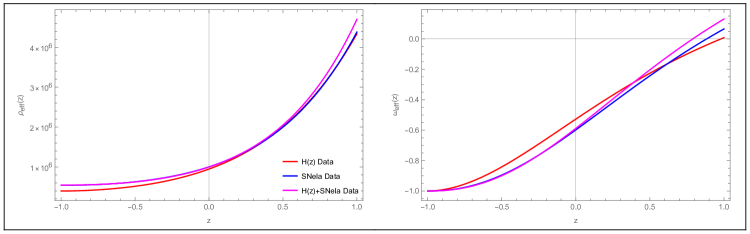
Figure 6: Effective energy density [Left panel] and effective EoS parameter [right panel] in redshift. The parameter scheme: $\alpha_{1}=-1$, $\beta_{1}=1$, $n=1.36$, $\Omega_{m}=0.3$ and $\Omega_{r}=0.00001$.

In a similar note, using Eq. (36), Eq. (21)-Eq.(23) can be written as,

$$p_{\rm eff} = \frac{1}{3}\Omega_{r}(z+1)^{4}-\frac{12(\alpha_{2}-1)\xi^{4}\left((z+1)^{\gamma}+\epsilon\right)^{4}\left((2\gamma-3)(z+1)^{\gamma}-3\epsilon\right)+\beta_{2}(2\gamma+3)(z+1)^{\gamma}+3\beta_{2}\epsilon}{12\xi^{2}\left((z+1)^{\gamma}+\epsilon\right)^{3}},$$ (40)

$$\rho_{\rm eff} = -3(\alpha_{2}-1)\xi^{2}\left((z+1)^{\gamma}+\epsilon\right)^{2}+\frac{\beta_{2}}{4\xi^{2}\left((z+1)^{\gamma}+\epsilon\right)^{2}}+\Omega_{m}(z+1)^{3}+\Omega_{r}(z+1)^{4},$$ (41)

$$\omega_{\rm eff} = \frac{\frac{1}{3}\Omega_{r}(z+1)^{4}-\frac{12(\alpha_{2}-1)\xi^{4}\left((z+1)^{\gamma}+\epsilon\right)^{4}\left((2\gamma-3)(z+1)^{\gamma}-3\epsilon\right)+\beta_{2}(2\gamma+3)(z+1)^{\gamma}+3\beta_{2}\epsilon}{12\xi^{2}\left((z+1)^{\gamma}+\epsilon\right)^{3}}}{-3(\alpha_{2}-1)\xi^{2}\left((z+1)^{\gamma}+\epsilon\right)^{2}+\frac{\beta_{2}}{4\xi^{2}\left((z+1)^{\gamma}+\epsilon\right)^{2}}+\Omega_{m}(z+1)^{3}+\Omega_{r}(z+1)^{4}}~{},$$ (42)

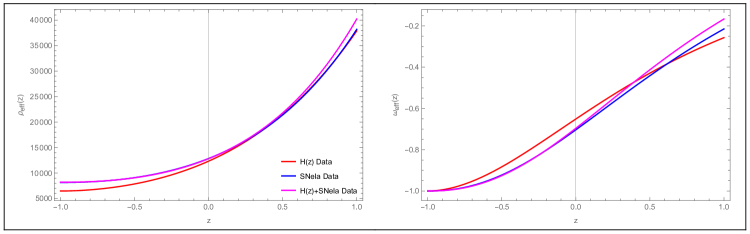
Figure 7: Effective energy density [left panel] and effective EoS parameter [right panel] in redshift. The parameter scheme: $\alpha_{2}=0.1$, $\beta_{2}=0.1$, $\Omega_{m}=0.3$ and $\Omega_{r}=0.00001$.

From FIG.-7, we can observe that the behavior of energy density decreases from early time to late time but does not vanish. The effective EoS parameter gives the present value as $(\omega_{\rm eff})_{0}\simeq-0.6515$, $(\omega_{\rm eff})_{0}\simeq-0.7033$ and $(\omega_{\rm eff})_{0}\simeq-0.6960$ for the constrained free parameters from $H(z)$ data set, $Pantheon+Analysis$ data set and combine $H(z)+Pantheon+Analysis$ data set respectively. The energy density and EoS are only dependent on the value of the coefficients of the model, which control the evolutionary aspects of the dynamical parameters. This model shows the quintessence behavior at the present time of its evolution.

VII Conclusions

In this work, we explored the viability of some symmetric teleparallel gravity-based models against the recent observational data sets such as the $Pantheon+Analysis$ data, $H(z)$ data, $H(z)+Pantheon+Analysis$ data, Baryon Acoustic Oscillations ($BAO$) data and Cosmic Microwave Background ($CMB$) distance priors. It is worth mentioning that the considered observational data are independent of any given cosmological model. Our main goal is to constrain the model parameters with these data and also compare the deviation from the standard $\Lambda$CDM scenario. To meet the goal, we employ the MCMC method with the Scipy optimization technique from the Python library.

After successfully implementing the MCMC process, we could extract the best-fit values of the cosmological free parameters. The obtained parameter values were found to be well-suited to the $BAO/CMB$ data sets. Also for each data set, we have analysed the behaviour of the deceleration parameter, which gives accelerating behaviour of the Universe and the $(j,~{}s)$ values which shows the Universe falls under the quintessence region. The present value of the cosmographic parameters are obtained with the constrained free parameters and are listed in TABLE 1.

Next, we used the best-fit parameters to investigate the physical viability of $f(Q)$ gravity models by analyzing the behavior of the effective energy density. We obtained that the cosmic energy density is non-negative and decreases from the early to the late universe. We also determine the evolution of the effective EoS, which shows a transition from a decelerated to an accelerated phase described by the models. Such feature exhibited by the $f(Q)$ models is appropriate to describe structure formation as well as the present dark energy domination. Moreover, in late time, the effective EoS approaches the cosmological constant limit i.e. $\omega_{\rm eff}=-1$. We wish to note here that DE and effective EoS parameters show similar behaviour in both models. It seems that dark energy EoS is dominating the evolutionary aspects of the models. Finally, we can remark that both the models support the quintessence behaviour at the present time and at late times, it approaches standard $\Lambda$CDM models.

In summary, our work shows that $f(Q)$ models can be considered as an alternative to the standard $\Lambda$CDM. Further, our results allow us to use other physically viable forms of $f(Q)$ to check the evolutionary behaviour of the Universe, which may provide some deep insight into the issue of late-time cosmic acceleration.

Table 2: The observational data sets that was used in [50].

No.	Redshift	H(z)	$\sigma_{H}$	Ref.	No.	Redshift	H(z)	$\sigma_{H}$	Ref.
1.	0.07	69.0	19.6	[60]	17.	0.4783	80.9	9.0	[63]
2.	0.09	69.0	12.0	[61]	18.	0.48	97	62	[65]
3.	0.12	68.6	26.2	[60]	19.	0.593	104	13	[62]
4.	0.17	83	8	[61]	20.	0.68	92	8	[62]
5.	0.179	75.0	4.0	[62]	21.	0.75	98.8	33.6	[66]
6.	0.199	75.0	5.0	[62]	22.	0.781	105	12	[62]
7.	0.200	72.9	29.6	[60]	23.	0.875	125	17	[62]
8.	0.27	77	14	[61]	24.	0.88	90	40	[65]
9.	0.28	88.8	36.6	[60]	25.	0.9	117	23	[61]
10.	0.352	83	14	[62]	26.	1.037	154	20	[62]
11.	0.38	83.0	13.5	[63]	27.	1.3	168	17	[61]
12.	0.4	95	17	[61]	28.	1.363	160	33.6	[67]
13.	0.4004	77	10.2	[63]	29.	1.43	177	18	[61]
14.	0.425	87.1	11.2	[63]	30	1.53	140	14	[61]
15.	0.445	92.8	12.9	[63]	31.	1.75	202	40	[61]
16.	0.47	89	49.6	[64]	32.	1.965	186.5	50.4	[67]

References

- [1] A.G. Riess et al., The Astronomical Journal, 116, 1009 (1998).
- [2] S. Perlmutter et al., The Astronomical Journal, 517, 565 (1999).
- [3] E. Komatsu et al., The Astrophysical Journal Supplement Series, 148, 119 (2003).
- [4] D.J. Eisenstein et al., The Astrophysical Journal, 633, 560 (2005).
- [5] S.F. Daniel et al., Physical Review D, 77, 105513 (2008).
- [6] E. Komatsu et al., The Astrophysical Journal Supplement Series, 192, 18 (2011).
- [7] G. Hinshaw, et al., The Astrophysical Journal Supplement Series, 208, 19 (2013).
- [8] S. Alam, et al., Monthly Notices of the Royal Astronomical Society, 470, 2617 (2016).
- [9] P.A.R. Ade, et al., Astronomy & Astrophysics., A13, 594 (2016).
- [10] N. Aghanim et al., Astronomy & Astrophysics, A1, 641 (2020).
- [11] R. Aldrovandi and J.G. Pereira, Teleparallel Gravity (Springer, Dordrecht, 2013), Vol. 173.
- [12] J.M. Nester et al., arXiv:gr-qc/9809049v2, (1999).
- [13] B. Altschul et al., Advances in Space Research 55, 501 (2015).
- [14] J.B. Jimenez et al., Physical Review D, 98, 044048 (2018).
- [15] J. Lu et al., European Physics Journal C, 79, 530 (2019).
- [16] R. Lazkoz et al., Physical Review D, 100, 104027 (2019).
- [17] J.B. Jimenez et al., Physical Review D, 101, 103507 (2020).
- [18] I. Ayuso et al., Physical Review D, 103, 063505 (2021).
- [19] F. Esposito et al., Physical Review D, 105, 084061 (2022).
- [20] N. Dimakis et al., Physical Review D, 106, 043509 (2022).
- [21] K. Hu et al., Physical Review D, 106, 044025 (2022).
- [22] W. Khyllep et al., Physical Review D, 103, 103521 (2021).
- [23] W. Khyllep et al., Physical Review D 107, 044022 (2023).
- [24] S. Sahlu et al., arXiv:2206.02517, (2022).
- [25] I. Soudi et al., Physical Review D 100, 044008 (2019).
- [26] B.J. Barros et al., Physics of the Dark Universe 30, 100616 (2020).
- [27] F.K. Anagnostopoulos et al., Physics Letters B, 822, 136634 (2021).
- [28] L. Atayde et al., Physical Review D, 104, 064052 (2021).
- [29] N. Frusciante, Physical Review D, 103, 044021 (2021).
- [30] F.K. Anagnostopoulos et al., European Physics Journal C, 83, 58 (2023).
- [31] S.A. Narawade et al., Physics of the Dark Universe, 36, 101020 (2022).
- [32] S.A. Narawade, B. Mishra, arXiv:2211.09701, (2022).
- [33] M. Koussour et al., Classical and Quantum Gravity, 39, 195021 (2022)., Annals of Physics, 445, 169092 (2022).
- [34] S.K. Maurya et al., Progress of Physics, 70, 2200061 (2022).
- [35] T. Harko et al., Physical Review D, 98, 084043 (2018).
- [36] S. Bahamonde et al., Journal of Cosmology and Astroparticle Physics, 08, 082 (2022).
- [37] S. Capozziello et al., Physics Letters B, 832, 137229 (2022).
- [38] L. Jarv et al., Physical Review D, 97, 124025 (2018).
- [39] M. Runkla, O. Vilson, Physical Review D, 98, 084034 (2018).
- [40] Y. Xu et al., European Physics Journal C, 79, 708 (2019).
- [41] T. Ortin, Gravity and Strings (2004).
- [42] R. Amanullah et al., The Astrophysical Journal, 716, 712 (2010).
- [43] N. Banerjee, Sudipta Das, General Relativity and Gravitation, 37, 1695 (2005).
- [44] S. Capozziello et al., Physics Letters B, 664, 12 (2008).
- [45] Y. Yang, Y. Gong, Journal of Cosmology and Astroparticle Physics, 06, 059 (2020).
- [46] S. Capozziello et al., Physical Review D, 90, 044016 (2014).
- [47] V. Sahni et al., Journal of Experimental and Theoretical Physics Letters, 77, 201 (2003).
- [48] U. Alam et al., Monthly Notices of the Royal Astronomical Society, 344, 1057 (2003).
- [49] F. Y. Wang et al., Astronomy and Astrophysics, 507, 53 (2009).
- [50] M. Moresco et al., Living Reviews in Relativity, 25, 6 (2022).
- [51] D. Brout et al., The Astrophysical Journal, 938, 110 (2022).
- [52] D.M. Scolnic et al., The Astrophysical Journal, 859, 101 (2018).
- [53] R. Giostri et al., Journal of Cosmology and Astroparticle Physics, 03, 027 (2012).
- [54] E. Komatsu et al., The Astrophysical Journal Supplement Series, 180, 330 (2009).
- [55] W. Percival et al., Monthly Notices of the Royal Astronomical Society, 401, 4 (2010).
- [56] F. Beutler et al., Monthly Notices of the Royal Astronomical Society, 416, 4 (2011).
- [57] C. Blake et al., Monthly Notices of the Royal Astronomical Society, 418, 3 (2011).
- [58] S. Capozziello, M. Shokri, Physics of the Dark Universe, 37, 101113 (2022).
- [59] M. Koussour et al., International Journal of Modern Physics D, 31, 16 (2022).
- [60] C. Zhang et al., Research in Astronomy and Astrophysics, 14, 1221, (2014).
- [61] J. Simon et al., Physical Review D, 71, 123001 (2005).
- [62] M. Moresco et al. Journal of Cosmology and Astroparticle Physics, 08, 006 (2012).
- [63] M. Moresco et al., Journal of Cosmology and Astroparticle Physics, 05, 014 (2016).
- [64] A.L. Ratsimbazafy et al., Monthly Notices of the Royal Astronomical Society, 467, 3 (2017).
- [65] D. Stern et al., Journal of Cosmology and Astroparticle Physics, 02, 008 (2010).
- [66] N. Borghi et al., The Astrophysical Journal Letters, 928, 1 (2022).
- [67] M. Moresco, Monthly Notices of the Royal Astronomical Society, 450, 1 (2015).