Spring: A High-Resolution High-Detail Dataset and Benchmark
for Scene Flow, Optical Flow and Stereo

Abstract

While recent methods for motion and stereo estimation recover an unprecedented amount of details, such highly detailed structures are neither adequately reflected in the data of existing benchmarks nor their evaluation methodology. Hence, we introduce Spring – a large, high-resolution, high-detail, computer-generated benchmark for scene flow, optical flow, and stereo. Based on rendered scenes from the open-source Blender movie “Spring”, it provides photo-realistic HD datasets with state-of-the-art visual effects and ground truth training data. Furthermore, we provide a website to upload, analyze and compare results. Using a novel evaluation methodology based on a super-resolved UHD ground truth, our Spring benchmark can assess the quality of fine structures and provides further detailed performance statistics on different image regions. Regarding the number of ground truth frames, Spring is 60$\times$ larger than the only scene flow benchmark, KITTI 2015, and 15$\times$ larger than the well-established MPI Sintel optical flow benchmark. Initial results for recent methods on our benchmark show that estimating fine details is indeed challenging, as their accuracy leaves significant room for improvement. The Spring benchmark and the corresponding datasets are available at http://spring-benchmark.org.

Figure 1: Illustration of the high amount of details in the Spring dataset. The dataset consists of HD images with super-resolved UHD ground truth for disparities and optical flow.

Table 1: Overview over recent datasets and benchmarks (BM). Where applicable, we report available image pairs and ground truth frames for motion estimation, i.e. scene flow (SF) or optical flow (OF), and for disparity estimation, i.e. stereo (ST), separately.

Venue SF OF ST BM   #image pairs ​#gt frames #pix scenes source ph.realism motion Spring (ours) CVPR ’23 ✓ ✓ ✓ ✓ 5953 6000 23812 12000 2.1M 47 CGI high realistic KITTI 2015 [30] CVPR ’15 ✓ ✓ ✓ ✓ 400 400 400 400 0.5M n/a real high automotive FlyingThings3D [28]​ CVPR ’16 ✓ ✓ ✓ ✗ 24084^‡ 26760^‡ 96336 53520 0.5M 2676 CGI low random VKITTI 2 [6] arXiv ’20 ✓ ✓ ✓ ✗ 21210 21260 84840 42520 0.5M 5 CGI med. automotive Monkaa [28] CVPR ’16 ✓ ✓ ✓ ✗ 8640^‡ 8664^‡ 34560 17328 0.5M 8 CGI low random Driving [28] CVPR ’16 ✓ ✓ ✓ ✗ 4392^‡ 4400^‡ 17568 8800 0.5M 1 CGI med. automotive KITTI 2012 [10] CVPR ’12 ✗ ✓ ✓ ✓ 389 389 389 389 0.5M n/a real high automotive MPI Sintel [5] ECCV ’12 ✗ ✓ (✓)${}^{*}\!\!\!$ ✓ 1593^‡ 1064^‡ 1593 1064 0.4M 35 CGI high realistic HD1K [22] CVPRW ’16 ✗ ✓ ✗ $\!\!\!{}^{\perp}$(✓)${}^{\dagger}\!\!\!$ 1074 n/a 1074 n/a 2.8M 63 real high automotive VIPER [34] ICCV ’17 ✗ ✓ ✗ ✓ 186285 n/a 372570 n/a 2.1M 184 CGI high automotive Middlebury-OF [2] IJCV ’11 ✗ ✓ ✗ ✓ 16 n/a 16 n/a 0.2M 16 HT/CGI med. small Human OF [33] IJCV ’20 ✗ ✓ ✗ ✗ 238900 n/a 238900 n/a 0.4M 18432 CGI med. rand./human AutoFlow [41] CVPR ’21 ✗ ✓ ✗ ✗ 40000 n/a 40000 n/a 0.3M n/a CGI low random FlyingChairs [8] ICCV ’15 ✗ ✓ ✗ ✗ 22872 n/a 22872 n/a 0.2M n/a CGI low random VKITTI [9] CVPR ’16 ✗ ✓ ✗ ✗ 21210 n/a 21210 n/a 0.5M 5 CGI low automotive Middlebury-ST [35] GCPR ’14 ✗ ✗ ✓ ✓ n/a 33 n/a 66 5.6M 33 real high n/a ETH3D [38] CVPR ’17 ✗ ✗ ✓ ✓ n/a 47 n/a 47 0.4M 11 real high n/a

HT: hidden texture, $\ddagger$: available in clean and final, $*$: not part of the benchmark, $\dagger$: offline

1 Introduction

The estimation of dense correspondences in terms of scene flow, optical flow and disparity is the basis for numerous tasks in computer vision. Amongst others, such tasks include action recognition, driver assistance, robot navigation, visual odometry, medical image registration, video processing, stereo reconstruction and structure-from-motion. Given this multitude of applications and their fundamental importance, datasets and benchmarks that allow quantitative evaluations have ever since driven the improvement of dense matching methods. The introduction of suitable datasets and benchmarks did not only enable the comparison and analysis of novel methods, but also triggered the transition from classical discrete [21, 12, 47] and continuous [13, 3, 4, 15, 31] optimization frameworks to current learning based approaches relying on neural networks [8, 42, 45, 53, 7, 46, 25]. The available benchmarks focus on distinct aspects like automotive scenarios [10, 30, 22, 34], differing complexity of motion [1, 2, 5] or (un)controlled illumination [35, 38]. However, none of these benchmarks provides a combination of high-quality data and a large number of frames, to assess a method’s quality in regions with fine details and to simultaneously satisfy the training needs of current neural networks. Furthermore, with KITTI2015 [30], only a single benchmark that goes back to the pre-deep-learning era is available for image-based scene flow, which currently prevents the development of well-generalizing methods due to lacking dataset variability.

Contributions. To tackle these challenges, we propose the Spring dataset and benchmark, providing a large number of high-quality and high-resolution frames and ground truths to enable the development of even more accurate methods for scene flow, optical flow and stereo estimation. With Spring, we complement existing benchmarks through a focus on high-detail data, while we simultaneously broaden the number of available datasets for the development of well-generalizing methods across data with varying properties. The latter aspect is particularly valuable for image-based scene flow methods. There, we provide the first benchmark with high-resolution, dense ground truth data in the literature. In summary, our contributions are fourfold:

1. New dataset: Based on the open-source Blender movie “Spring”, we rendered 6000 stereo image pairs from 47 sequences with state-of-the-art visual effects in HD resolution (1920$\times$1080px). For those image pairs, we extracted ground truth from Blender in forward and backward direction, both in space and time, amounting to 12000 ground truth frames for stereo and 23812 ground truth frames for motion – 60$\times$ more than KITTI and 15$\times$ more than MPI Sintel.

2. High-detail evaluation methodology: To adequately assess small details at a pixel level, we propose a novel evaluation methodology that relies on an even higher resolved ground truth. All ground truth frames are computed in UHD resolution (3840$\times$2160px).

3. Benchmark: We set up a public benchmark website to upload, analyze and compare novel methods. It provides several widely used error measures and additionally analyzes the results in different types of regions, including high-detail, unmatched, non-rigid, sky and large-displacement areas.

4. Baselines: We evaluated 15 state-of-the-art methods(8 optical flow, 4 stereo, 3 scene flow) as non-finetuned baselines. Results not only show that small details still pose a problem to recent methods, but also hint at significant potential improvements in all tasks.

Figure 2: Ground truth comparison for highly-detailed regions across datasets. From left to right: KITTI 15 [30], MPI Sintel [5], Spring.

2 Related work

In the literature there exists a large number of datasets and benchmarks for dense matching covering scene flow, optical flow and stereo. An overview over the state of the art is given in Tab. 1. Datasets and benchmarks can roughly be divided along two orthogonal axes: The scene axis and the data axis. On one edge of the scene axis, there are datasets focusing on automotive scenes such as KITTI [10, 30], Virtual KITTI [9, 6], HD1K [22], VIPER [34] and Driving [28]. On the other edge are datasets that target general scenes such as Middlebury [1, 35], MPI Sintel [5], ETH3D [38], FlyingThings3D [28], Monkaa [28] and FlyingChairs [8] with the special case of Human OF [33] that addresses human body motion. Along the orthogonal data axis, datasets and benchmarks can be divided into real-world data [10, 30, 22, 35, 38] and synthetic data [5, 34, 28, 8, 9, 33, 41]. In the context of optical flow, Sintel showed that synthetic benchmarks can validly approximate the statistics of natural images and motion, while avoiding ground truth measurements in the real world. This motivates the use of synthetic data for general scenes in our Spring dataset.

Resolution. Most of the benchmarks and datasets are limited to images with QHD resolution (0.5 Mpix) or below [10, 30, 5, 28, 8, 38, 33, 41, 11]. Only in the case of automotive optical flow, full HD resolution (2-3 Mpix) has been considered [22, 34]. Moreover, first attempts with image sizes beyond HD (5.6 Mpix) have been made for real-world stereo, but only for a small number of images [35]. With respect to general optical flow and scene flow, Spring is the first dataset to consider HD resolution and above for input images and ground truth, respectively.

Dataset size. Considering the number of input and ground truth images, most popular benchmarks have at most 1600 frames. This is either due to the use of real-world footage [10, 35, 30, 22, 38] or their creation in the pre-deep-learning era [10, 5, 30]. The only exception is the automotive optical flow benchmark VIPER [34], if we leave aside several large training datasets without benchmark functionality such as FlyingChairs [8], Virtual KITTI [9, 6], FlyingThings3D with Monkaa and Driving [28], Human OF [33], AutoFlow [41] and the dataset generator Kubric  [11]. With respect to the number of frames for stereo and scene flow, however, Spring is the first general-scene benchmark with several thousand samples for training and testing, closing a previously existing gap in the available training data for deep-learning matching methods for those tasks.

Benchmark evaluation. Regarding focused evaluations in particularly important regions, current benchmarks mainly focus on occlusions (unmatched regions) [2, 5, 30, 35, 38], discontinuities [1, 5], large displacements [5] and non-rigid areas [30]. However, recent stereo [23] and optical flow methods [19, 18] achieve highly detailed results due to cascaded recurrent neural networks that process images at larger resolutions and omit a significant upsampling of the final results (e.g. in contrast to [45, 20, 24]). This raises the question how well such high-quality methods can estimate fine-scale details such as grass or hair. In this context, Spring not only provides high-resolution images that contain small-scale details at pixel level, but also provides a novel evaluation methodology that allows to measure the accuracy in the presence of thin structures. Therefore, the Spring benchmark provides focused evaluations for regions with unmatched, high-detail, non-rigid, sky and large-displacement pixels.

Scene flow benchmarking. Finally, with only 400 frames, KITTI 2015 [30] is the only benchmark that, besides optical flow and stereo, also allows the evaluation of scene flow. Moreover, while there are a few datasets and challenges for scene flow from RGB-D [40, 39, 26] and LiDAR [43] data, KITTI 2015 is the only benchmark for image-based scene flow, i.e. scene flow only from stereo image pairs. As a consequence, recent image-based scene flow methods perform well on KITTI 2015 but are likely not robust under other types of data. As shown for optical flow and stereo in context of the Robust Vision Challenge [52], improving the generalization across benchmarks is essential to increase applicability and robustness [37]. Hence, having more specifically tailored benchmarks at hand would not only be beneficial for optical flow and stereo, but in particular for image-based scene flow, where they are indispensable to further advance research. While with FlyingThings3D, Monkaa and Driving [28] as well as VKITTI 2 [6] there are a few datasets available that could also be used for benchmarking, these datasets provide the ground truth for all frames which encourages overfitting. In contrast, Spring offers the full benchmark functionality, i.e. hidden ground truth for the test set, an evaluation protocol, cheating prevention and a website to compare results.

3 Spring dataset

The Spring dataset is a novel, large, computer-generated dataset for training and evaluating scene flow, optical flow and stereo methods. Our dataset consists of stereoscopic video sequences and ground truth scene flow in its standard parametrization with reference frame disparity, target frame disparity and optical flow [15]. We provide ground truth data for all available combinations; for the left and right view as well as motion in temporal forward and backward direction. The Spring dataset is based on the open-source movie “Spring”, which we utilize to generate a large dataset that is suitable for motion and disparity estimation. In the following, we introduce the underlying movie data, give details on the dataset creation process and provide a full overview of our data along with a comparison to other established datasets.

3.1 Open-source movie data

We retrieve our data from an open movie project generated in the open-source 3D software Blender. The core idea of open movies is to make all assets that are required to render the movie available under an open license, which enables anybody to build upon the creative work and to utilize it for research [5, 28, 17]. The “Spring” movie is a recent project showcasing the current progress in Blender 2.80 and the ray tracing engine Cycles and is with its scenes and assets available under the open CC BY 4.0 license. The movie scenes depict a large range of shot sizes from extreme close-ups to very long shots and a large range of motions from animated creatures, flight sequences, chasing motion, plant growth, and physically plausible simulations of pebbles, grass and hair motion. It shows advanced visual effects that work towards a realistic appearance of the computer-generated data, such as 3D motion blur and camera depth of field with focus pulls (changes of the focal plane). Some scenes even contain zooms (changes of the focal length, i.e. frame-dependent camera intrinsics), which makes our dataset the first scene flow dataset [30, 28, 6] with this property. In general, all movie assets are highly detailed, see e.g. Figs. 1 and 2 which provides a good basis for our datasets.

Figure 3: Examples for evaluation maps. Top row: Sky map, detail map, bottom row: unmatched regions map, non-rigid motion map.

Figure 4: Example sequences from the Spring dataset. First row: Left and right images of the stereo camera, second row: Corresponding left and right disparity, third row: Change in disparity for forward left, backward left, forward right and backward right, fourth row: Optical flow visualization for forward left, backward left, forward right and backward right. Please note that we show the disparity change for visualization purposes while the dataset contains the target frame disparity.

3.2 Dataset creation

We consider a set of 47 scenes with 6000 frames covering large parts of the original movie. In each scene, the original monoscopic camera is replaced by a stereoscopic camera with a baseline distance of 6.5 cm. While keeping the original appearance of the scenes, we had to introduce changes to make them suitable for dataset creation: Where applicable, we removed dense volumetric clouds, since Blender cannot generate ground truth for them, but kept ambient haze.

We then generated the data in four steps: First, we rendered the image data in HD resolution with 1920$\times$1080px, including all visual effects. Second, we generated all data that is required for the ground truth computation, where we disabled motion blur and depth of field and set all objects to solid. Third, we considered sky regions separately, since Blender is not able to compute ground truth for these regions. Fourth, we computed additional maps for an improved analysis of results in terms of focused evaluations. For each step, more details are given below.

High-detail structures. Up to now, datasets in the literature were not able to represent very thin structures such as hair, grass, or any objects that are smaller than 1px due to the definition of disparities and optical flow as a single representation per pixel. To mitigate this, [5, 48] proposed to change the rendering data such that hair is at least 2px wide, which significantly changes the visual appearance. We propose a novel solution to this problem by generating all ground truth data with twice the spatial resolution, which yields four ground truth values for each image pixel and a total resolution of 3840$\times$2160px. This way, even fine details like hair or grass are represented in the data, see Fig. 2. We describe how to use this high-resolution data for evaluation in Sec. 4.1.

Ground truth scene flow from Blender. Since it is not possible to directly export 3D motion or scene flow from Blender, we first had to adapt the rendering source code. We modified it such that we were able to output 3D motion vectors relative to the camera coordinate system. Then, we extracted forward and backward 3D motion vectors and depth, for both the left and the right camera. Additionally, we saved the intrinsic and extrinsic camera data as well as the focal distance. From depth, 3D motion and camera data, it is straightforward to compute ground truth scene flow in the standard parametrization with reference disparity, future/past disparity and optical flow [15]. We make the code required to generate our dataset with scene flow ground truth from Blender publicly available.

Sky areas. In several recent datasets, sky areas are not included [34, 30, 10], yielding a sparse ground truth for many sequences. Also, the Blender rendering engine is not capable of determining the correct motion vectors for infinitely distant sky points. Thus, one mitigation strategy is to create a large sphere around the scene [28, 27] to obtain motion results for every pixel. While this provides a reasonable approximation, we opted for an actual computation of the ground truth scene flow in sky regions. For the optical flow, we utilized the relative camera motion to compute the true 2D displacement vectors for pixels of infinite depth, which comes down to considering the rotational part of the relative camera motion only. For the disparities, the ground truth values are given as 0. In order to allow for a separate evaluation, we created binary maps determining sky pixels.

Additional maps. Apart from sky maps, we computed three additional maps to enable a detailed evaluation with our benchmark: high-detail, matching, and rigidity maps; see Fig. 3. In the evaluation, we further distinguished between areas of different displacement vector sizes. In the following, we describe their generation.

A core concept in our dataset is to have the ground truth data available in super-resolution with four ground truth values per pixel. We use this high-resolution data to compute detail maps to identify pixels that belong to areas of high details for all scene flow components, i.e. optical flow and disparities. To this end, we define a point as high-detail if at least one of the four ground truth values deviates from the median of the four ground truth values by more than 1px.

Additionally, we compute matching maps to differentiate pixels that are matched in the corresponding view from those that are occluded. This idea has been frequently used [10, 30, 5, 36, 38] and is especially important to distinguish regions with matching counterparts from regions where values have to be predicted/extrapolated. We computed matching maps for all scene flow components through a forward-backward check [44].

Further, we calculate rigidity maps that segment the data into areas where motion is induced only by the camera and areas where objects move independent of the camera. Instead of computing rigidity maps in 2D [49], we determine them in 3D by comparing the ground truth 3D motion vectors to 3D motion vectors that are computed from the static scene and the camera motion. This 3D strategy prevents errors which are otherwise introduced by comparing projected vectors in 2D. We consider points to be rigid if the 3D motion vectors differ by at most 1mm.

Finally, we also distinguish areas of different displacement sizes for all scene flow components. Following [5] we select regions of small-size displacements with magnitudes up to 10px (s0-10), regions of medium-size displacements with magnitudes of 10-40px (s10-40) and regions of even larger displacements exceeding 40px (s40+).

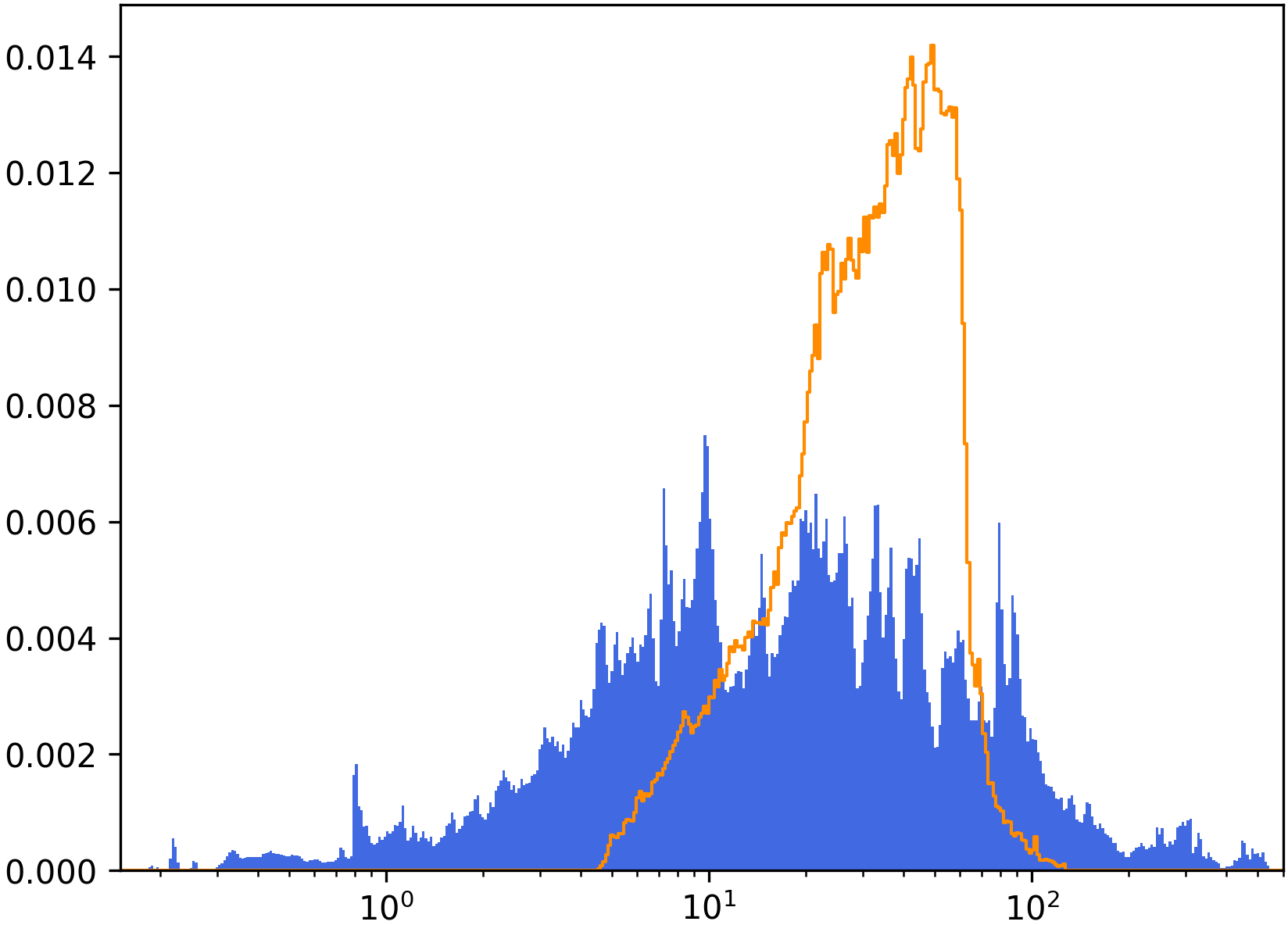
(a) Reference disparity

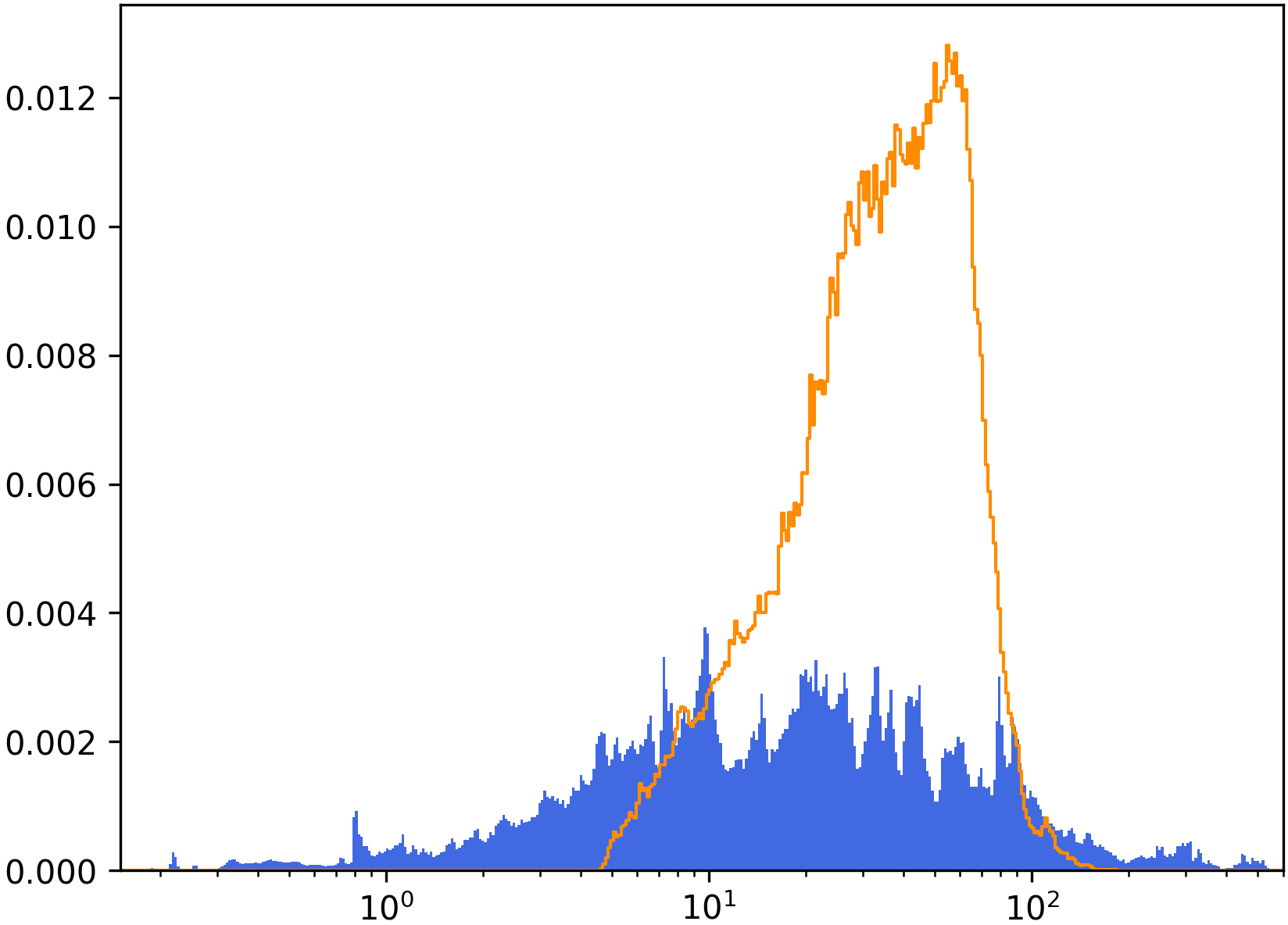
(b) Target disparity

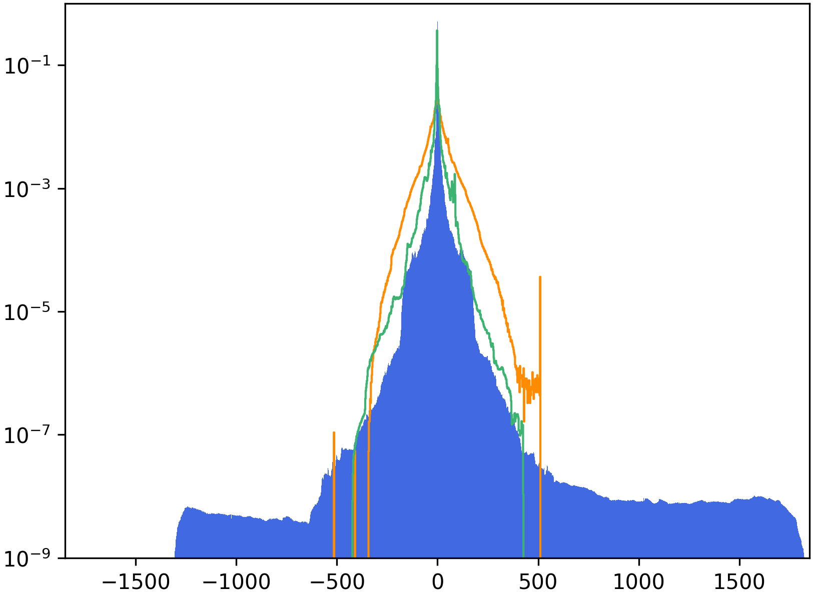
(c) Optical flow $u$ component

(d) Optical flow $v$ component

Figure 5: Comparison of ground truth statistics between the datasets Spring (blue) and KITTI 2015 (orange) and Sintel (green).

3.3 Dataset Overview

Our dataset consists of 47 scenes, which we used to render a total of 6000 stereo frame pairs. For each left and right frame, we generate disparity ground truth as well as forward and backward optical flow and scene flow ground truth. In every sequence, we omit the backward flow at the first frame and the forward flow at the last frame. Thus, considering left/right and forward/backward pairs, our dataset consists of 23812 data samples for scene flow and optical flow and 12000 data samples for stereo estimation. Figure 5 compares the distribution of disparity and optical flow values with the KITTI 15 [30] and MPI Sintel [5] datasets. Regarding optical flow, Spring employs a wider range of motion vectors, including very large displacements. In contrast, for stereo, Spring not only contains larger disparities (very close objects), but also a significant amount of small disparities (far-away objects).

4 Benchmark

We split the 47 sequences of our dataset into 37 train and 10 test sequences, yielding 5000 and 1000 stereo frames, respectively. We make the full data of the train split available, but only publish the images for the test split while withholding the ground truth files, which is a standard practise [2, 34, 30, 10, 5, 36]. In order to allow for a fair comparison, we create a public benchmark website where authors can upload their test split results. The results are automatically evaluated, with optional display in a public ranking. Following other benchmarks [5, 34], we make use of a subsampling strategy to reduce the file size of test split results prior to uploading to the benchmark. We make the entire code of our benchmark website publicly available.

Table 2: Optical flow results on Spring. We show the 1px outlier rate with sub-rankings for low/high-detail, (un)matched, (non-)rigid and (not) sky regions. Additionally, we show the average endpoint error (EPE), the Fl error [30] as well as the WAUC metric [34].

	1px												EPE	Fl	WAUC
Method	total	low-det.	high-det.	matched	unmat.	rigid	non-rig.	not sky	sky	0s0-10	s10-40	s40+0
MS-RAFT+ [19, 18]	05.72	05.37	61.50	05.04	33.95	3.05	25.97	04.84	19.15	02.06	05.02	38.32	0.643	02.19	92.89
FlowFormer [14]	06.51	06.14	64.22	05.77	37.29	3.53	29.08	05.50	21.86	03.38	05.53	35.34	0.723	02.38	91.68
FlowNet2 [16]	06.71	06.35	64.06	05.69	48.89	3.71	29.40	06.04	16.91	01.86	05.82	49.69	1.040	02.82	90.91
RAFT [45]	06.79	06.43	64.09	06.00	39.48	4.11	27.09	05.25	30.18	03.13	05.30	41.40	1.476	03.20	90.92
GMA [20]	07.07	06.70	66.20	06.28	39.89	4.28	28.25	05.61	29.26	03.65	05.39	40.33	0.914	03.08	90.72
GMFlow [51]	10.36	09.93	76.61	09.06	63.95	6.80	37.26	08.95	31.68	05.41	09.90	52.94	0.945	02.95	82.34
SPyNet[32]	29.96	29.66	77.45	28.78	78.77	26.44	56.60	25.83	92.74	24.80	24.20	88.71	4.162	12.87	67.15
PWCNet[42]	82.27	82.27	81.75	82.07	90.40	82.82	78.09	81.57	92.76	81.40	82.19	89.69	2.288	04.89	45.67

Table 3: Stereo results on Spring. We show the 1px outlier rate with sub-rankings for low/high-detail, (un)matched, and (not) sky regions. Additionally, we show the absolute error (Abs), and the D1 error [30].

	1px										Abs	D1
Method	total	low-detail	high-detail	matched	unmatched	not sky	sky	s0-10	s10-40	s40+
ACVNet [50]	14.77	14.43	35.27	12.60	57.89	11.16	69.62	18.39	11.35	18.15	1.52	05.35
RAFT-Stereo [24]	15.27	14.98	32.77	13.39	52.58	09.92	96.57	22.59	10.02	17.09	3.02	08.63
LEAStereo[7]	19.89	19.55	40.40	17.61	65.09	16.73	67.81	19.08	13.86	39.41	3.88	09.19
GANet [53]	23.22	22.91	42.06	20.98	67.88	18.42	96.27	24.29	16.43	41.50	4.59	10.39

Table 4: Scene flow results on Spring. We show the 1px outlier rate with sub-rankings for low/high-detail, (un)matched, (non-)rigid and (not) sky regions. Additionally, we show the SF error [30] as well as individual 1px outlier rates for reference disparity (1px${}^{\text{D1}}$), target disparity (1px${}^{\text{D2}}$) and optical flow (1px${}^{\text{Fl}}$).

	1px												SF	1px${}^{\text{D1}}$	1px${}^{\text{D2}}$	1px${}^{\text{Fl}}$
Method	total	low-det.	high-det.	matched	unmat.	rigid	non-rig.	not sky	sky	s0-10	s10-40	s40+
M-FUSE (F) [29]	34.90	34.30	64.32	32.03	71.94	29.81	73.38	31.36	88.71	29.89	23.91	69.15	16.10	19.89	24.26	20.37
RAFT-3D (K) [46]	37.26	36.80	60.23	34.34	75.02	32.87	70.52	33.23	98.53	43.80	24.55	63.91	17.35	32.31	32.95	13.96
CamLiFlow (F) [25]	50.08	49.64	71.88	47.80	79.64	46.75	75.27	46.85	99.25	31.12	42.70	89.55	34.15	23.22	44.10	24.01
M-FUSE (K) [29]	62.49	62.29	72.31	60.57	87.25	60.39	78.42	60.03	99.85	49.20	75.96	25.23	25.23	52.23	57.03	20.98
RAFT-3D (F) [46]	78.82	78.75	82.20	78.33	85.19	79.62	72.80	77.57	97.84	84.33	81.68	65.48	66.88	23.22	73.43	48.07
CamLiFlow (K) [25]	85.31	85.18	91.67	84.46	96.25	84.18	93.85	84.35	99.96	65.16	87.85	99.86	70.87	32.31	76.32	69.68

Table 5: Influence of the subsampling on the evaluation. We compare optical flow results evaluated using the subsampling of the benchmark with the same results evaluated on the full test split.

	subsampling results				full test split results
	1px	EPE	Fl		1px	EPE	Fl
MS-RAFT+ [19, 18]	05.72	0.643	02.19		04.99	0.620	01.82
FlowFormer [14]	06.51	0.723	02.38		06.12	0.719	02.18
FlowNet2 [16]	06.71	1.040	02.82		05.91	0.968	02.30
RAFT [45]	06.79	1.476	03.20		06.05	1.265	02.72
GMA [20]	07.07	0.914	03.08		06.30	0.918	02.69
GMFlow [51]	10.36	0.945	02.95		09.38	0.928	02.49
SPyNet[32]	29.96	4.162	12.87		28.72	4.036	11.95
PWCNet [42]	82.27	2.288	04.89		82.17	2.295	04.47

4.1 Evaluation metrics

As described in Sec. 3, we generate the ground truth data in double resolution, resulting in four ground truth values per pixel. Out of these, the evaluation always selects the ground truth value closest to the estimated value for calculating the errors. In the case of of thin hair structures against a background, this strategy yields a low error for methods that estimate the hair or the background value, while assigning a larger error when a mixture of both values is predicted.

In the literature, there is a multitude of error measures for scene flow, optical flow and stereo methods. For scene flow, the most established ones are the outlier rates by KITTI. They define pixels as outliers if they deviate by more than 3px and 5% from the ground truth, which is motivated from the limited precision of their data [30]. Considering our high-accuracy data, we adapt the evaluation to the 1px outlier rate. For reference disparity, target disparity and optical flow, the 1px outlier rate defines the percentage of pixels that deviate more than 1px from the ground truth. Following [30], we also employ a union 1px error as the main scene flow measure that defines the percentage of pixels where any of the estimated reference disparity, target disparity and optical flow values deviates more than 1px from the ground truth. Since for scene flow, optical flow and stereo no single error measure is fully established in the community, we also provide multiple error metrics as additional reference. For stereo, we also show the absolute error and the KITTI-D1 and D2 error [30]; for optical flow, we show the end point error, the KITTI-Fl error and the WAUC error [34]; for scene flow, we show all previously mentioned errors as well as the KITTI-SF error [30]. To enable an in-depth analysis, we make use of the maps described in Sec. 3.2 and additionally report sub-errors for different parts of the scene.

4.2 Rules and cheating prevention

Our cheating prevention strategy is threefold. First, we require authors to register on our website giving their affiliation and a brief justification why they need access to the benchmark. After verification of the account, which shall prevent mass-registration, authors are allowed to submit results under upload limits [5, 30]: At most once per hour and three times per 30 days. This way, we prevent overfitting on the test data. Second, we added several sequences with manual adjustment of the camera path [5] in our data generation process to prevent users from utilizing the publicly available movie assets. Third, we make our full benchmark code publicly available, but hide the exact subsampling used for generating the submission files by only providing compiled subsampling executables.

4.3 Initial results

For evaluation on our benchmark, we consider 15 state-of-the-art methods (8 optical flow, 4 stereo, 3 scene flow) whose code is publicly available. The results are given in Tabs. 4, 2 and 3. We selected author-provided checkpoints trained on Sintel for optical flow, on FlyingThings3D for stereo, and on both FlyingThings3D and KITTI for scene flow. We argue that, at the initial stage, an evaluation of methods that are not finetuned on Spring results in a fairer comparison than retraining methods of other authors on the train split of our dataset. Moreover, using non-finetuned methods also gives interesting insights into the generalization performance of existing methods to novel benchmarks. At the same time, it is clear that these results and rankings can only serve as starting point. Hence, we encourage authors to submit finetuned versions of their methods to our benchmark. In the following, we give an initial discussion of our results, which is extended in the supp. material.

Optical flow. For optical flow, we can observe that although recent methods perform generally well, errors in areas with high details are still very large – although our novel evaluation method is quite permissive in those areas. Furthermore, we find that the errors in unmatched, non-rigid, sky and large-displacement areas are also large with the error in the sky being actually the smallest. Among the different methods, MS-RAFT+ [18], which is specifically tailored for high resolutions and single-checkpoint cross-benchmark generalization [52], ranks first. Moreover, the classical FlowNet2 [16] performs surprisingly well which can be attributed to its dedicated module for small displacement estimation (cf. the s0-10 metric). In contrast, the well-established PWCNet [42] ranks last. While it provides reasonable results in terms of the EPE and Fl error, its accuracy seems to be limited by its strategy to operate on 1/4 of the input resolution and subsequently upsample the flow using simple bilinear interpolation. Overall, these observations demonstrate that for Spring, the capability of the underlying architecture to handle high-detail high-resolution input is much more important than for other benchmarks. This in turn outlines the value of Spring when it comes to further pushing the limits of current optical flow methods.

Stereo. For stereo estimation, we can see that results are generally worse compared to optical flow. While surprising at first sight, we attribute this to mainly two reasons. First, most stereo methods consider very clean data, i.e. data without camera defocus and/or motion blur, which stands in contrast to our dataset. Second, stereo disparity is often defined to be strictly positive [10, 30, 28], thus in general stereo methods are not prepared for regions with zero disparity/infinite depth as for the sky in our dataset – which can be seen in the corresponding sub-metric, as well as the s0-10 metric. However, we argue that disparity methods, and subsequently scene flow methods, should be able to predict true dense fields, including sky regions. For reference, we provide a full evaluation solely on non-sky pixels for all methods including optical flow and scene flow in the supp. material. As a final note, previous stereo benchmarks often report results by default in non-occluded (matched) regions only [38, 10, 36, 35], which drives the development of methods that perform especially well in these areas. All in all, these results clearly demonstrate the advantage of the Spring benchmark for the field of stereo estimation.

Scene flow. For scene flow estimation, we evaluated two trained models for each method, corresponding to a pre-training on FlyingThings3D (F) and a subsequent finetuning on KITTI 2015 (K). Since the considered scene flow methods strongly rely on a preceding disparity estimation, the same observations hold as in case of the stereo results. Furthermore, the inconsistent results of all three methods with their two training schedules show that solely focusing on the KITTI 2015 benchmark produces methods that are prone to overfitting and lack a good generalization performance. Hence, the Spring benchmark is also highly beneficial to advance research in the field of scene flow.

4.4 Influence of subsampling

As previously outlined, our benchmark uses a subsampling strategy that evaluates on a reduced set of ground truth pixels from the full test set. In a final experiment, we investigate the influence of this strategy by comparing the subsampling results shown in Tab. 2 to results computed on the full test split. This is the first time in the dense matching literature that the influence of the subsampling evaluation is made transparent. Table 5 shows that evaluating with our subsampling yields similar results to using all ground truth pixels with the same or almost the same ranking – independent of the error measure.

5 Conclusion

With Spring, we present a large, high-resolution, high-detail, computer-generated dataset and benchmark for dense matching. Spring addresses the increasing performance of recent methods in terms of details, by allowing an adequate assessment in high-detail regions during evaluation. To this end, it provides 6000 photo-realistic HD stereo frame pairs with 23812 and 12000 super-resolved UHD ground truth frames for motion and stereo, respectively. Unlike several other benchmarks for matching tasks, Spring not only covers optical flow or disparity estimation: It is the first benchmark in the deep learning era that also evaluates image-based scene flow, which is essential to enable further progress in this field. Initial results of 15 non-finetuned baselines show that Spring is a challenging benchmark for recent methods – particularly with respect to high-detail, non-rigid, unmatched and sky regions.

Acknowledgements. The Spring movie assets by BlenderFoundation $|$ cloud.blender.org/spring are licensed under CC BY 4.0. We thank Andy Goralczyk, Francesco Siddi and the Blender Studio team. Lukas Mehl acknowledges funding by the Deutsche Forschungsgemeinschaft (DFG, German Research Foundation) – Project-ID 251654672 – TRR 161 (B04). Jenny Schmalfuss and Azin Jahedi acknowledge support from the International Max Planck Research School for Intelligent Systems (IMPRS-IS).

References

- [1] Simon Baker, Daniel Scharstein, J. P. Lewis, Stefan Roth, Michael J. Black, and Richard Szeliski. A database and evaluation methodology for optical flow. In Proc. IEEE International Conference on Computer Vision (ICCV), 2007.
- [2] Simon Baker, Daniel Scharstein, J. P. Lewis, Stefan Roth, Michael J. Black, and Richard Szeliski. A database and evaluation methodology for optical flow. International Journal of Computer Vision (IJCV), 92(1):1–31, 2011.
- [3] Michael J. Black and P. Anandan. The robust estimation of multiple motions: parametric and piecewise-smooth flow fields. Computer Vision and Image Understanding (CVIU), 63(1):75–104, 1996.
- [4] Thomas Brox, Andrés Bruhn, Nils Papenberg, and Joachim Weickert. High accuracy optical flow estimation based on a theory for warping. In Proc. European Conference on Computer Vision (ECCV), pages 25–36, 2004.
- [5] Daniel J. Butler, Jonas Wulff, G. B. Stanley, and Michael J. Black. A naturalistic open source movie for optical flow evaluation. In Proc. European Conference on Computer Vision (ECCV), pages 611–625, 2012.
- [6] Yohann Cabon, Naila Murray, and Martin Humenberger. Virtual KITTI 2. In arXiv preprint 2001.10773, 2020.
- [7] Xuelian Cheng, Yiran Zhong, Mehrtash Harandi, Yuchao Dai, Xiaojun Chang, Hongdong Li, Tom Drummond, and Zongyuan Ge. Hierarchical neural architecture search for deep stereo matching. In Proc. Conference on Neural Information Processing Systems (NeurIPS), pages 22158–22169, 2020.
- [8] Alexey Dosovitskiy, Philipp Fischer, Eddy Ilg, Caner Hazirbas, Vladimir Golkov, Patrick van der Smagt, Daniel Cremers, and Thomas Brox. Flownet: Learning optical flow with convolutional networks. In Proc. IEEE/CVF International Conference on Computer Vision (ICCV), pages 2758–2766, 2015.
- [9] Adrien Gaidon, Qiao Wang, Yohann Cabon, and Eleonora Vig. Virtual worlds as proxy for multi-object tracking analysis. In Proc. IEEE/CVF Conference on Computer Vision and Pattern Recognition (CVPR), pages 4340–4349, 2016.
- [10] Andreas Geiger, Philip Lenz, and Raquel Urtasun. Are we ready for autonomous driving? the KITTI vision benchmark suite. In Proc. Conference on Computer Vision and Pattern Recognition (CVPR), pages 3354–3361, 2012.
- [11] Klaus Greff, Francois Belletti, Lucas Beyer, Carl Doersch, Yilun Du, Daniel Duckworth, David J. Fleet, Dan Gnanapragasam, Florian Golemo, Charles Herrmann, Thomas Kipf, Abhijit Kundu, Dmitry Lagun, Issam Laradji, Liu Hsueh-Ti, Henning Meyer, Yishu Miao, Derek Nowrouzezahrai, Cengiz Oztireli, Etienne Pot, Noha Radwan, Daniel Rebain, Sara Sabour, Mehdi S. M. Sajjadi, Matan Sela, Vincent Sitzmann, Austin Stone, Deqing Sun, Suhani Vora, Ziyu Wang, Tianhao Wu, Kwang Moo Yi, Fangcheng Zhong, and Andrea Tagliasacchi. Kubric: A scalable dataset generator. In Proc. IEEE/CVF Conference on Computer Vision and Pattern Recognition (CVPR), 2022.
- [12] Heiko Hirschmueller. Accurate and efficient stereo processing by semi-global matching and mutual information. In Proc. IEEE Conference on Computer Vision and Pattern Recognition (CVPR), 2005.
- [13] Berthold K. P. Horn and Brian G. Schunck. Determining optical flow. In Proc. Techniques and Applications of Image Understanding, volume 0281, pages 319–331. International Society for Optics and Photonics, SPIE, 1981.
- [14] Zhaoyang Huang, Xiaoyu Shi, Chao Zhang, Qiang Wang, Ka Chun Cheung, Hongwei Qin, Jifeng Dai, and Hongsheng Li. FlowFormer: a transformer architecture for optical flow. In Proc. European Conference on Computer Vision (ECCV), 2022.
- [15] Frédéric Huguet and Frédéric Devernay. A variational method for scene flow estimation from stereo sequences. In Proc. IEEE International Conference on Computer Vision (ICCV), pages 1–7, 2007.
- [16] Eddy Ilg, Nikolaus Mayer, Tonmoy Saikia, Margret Keuper, Alexey Dosovitskiy, and Thomas Brox. FlowNet 2.0: Evolution of optical flow estimation with deep networks. In Proc. IEEE/CVF Conference on Computer Vision and Pattern Recognition (CVPR), pages 2462–2470, 2017.
- [17] Woobin Im, Sebin Lee, and Sung-Eui Yoon. Semi-supervised learning of optical flow by flow supervisor. In Proc. European Conference on Computer Vision (ECCV), 2022.
- [18] Azin Jahedi, Maximilian Luz, Lukas Mehl, Marc Rivinius, and Andrés Bruhn. High resolution multi-scale RAFT (Robust Vision Challenge 2022). In arXiv preprint 2210.16900. arXiv, 2022.
- [19] Azin Jahedi, Lukas Mehl, Marc Rivinius, and Andrés Bruhn. Multi-scale RAFT: Combining hierarchical concepts for learning-based optical flow estimation. In Proc. IEEE International Conference on Image Processing (ICIP), pages 1236–1240, 2022.
- [20] Shihao Jiang, Dylan Campbell, Yao Lu, Hongdong Li, and Richard Hartley. Learning to estimate hidden motions with global motion aggregation. In Proc. IEEE/CVF International Conference on Computer Vision (ICCV), 2021.
- [21] Vladimir Kolmogorov and Ramin Zabih. Multi-camera scene reconstruction via graph cuts. In Proc. European Conference on Computer Vision (ECCV), 2002.
- [22] Daniel Kondermann, Rahul Nair, Katrin Honauer, Karsten Krispin, Jonas Andrulis, Alexander Brock, Burkhard Gussefeld, Mohsen Rahimimoghaddam, Sabine Hofmann, Claus Brenner, et al. The HCI benchmark suite: Stereo and flow ground truth with uncertainties for urban autonomous driving. In Proc. IEEE/CVF Conference on Computer Vision and Pattern Recognition Workshops (CVPRW), pages 19–28, 2016.
- [23] Jiankun Li, Peisen Wang, Pengfei Xiong, Tao Cai, Ziwei Yan, Lei Yang, Jiangyu Liu, Haoqiang Fan, and Shuaicheng Liu. Practical stereo matching via cascaded recurrent network with adaptive correlation. In Proc. IEEE/CVF Conference on Computer Vision and Pattern Recognition (CVPR), 2022.
- [24] Lahav Lipson, Zachary Teed, and Jia Deng. RAFT-Stereo: Multilevel recurrent field transforms for stereo matching. In International Conference on 3D Vision (3DV), 2021.
- [25] Haisong Liu, Tao Lu, Yihui Xu, Jia Liu, Wenjie Li, and Lijun Chen. CamLiFlow: Bidirectional camera-LiDAR fusion for joint optical flow and scene flow estimation. In Proc. IEEE/CVF Conference on Computer Vision and Pattern Recognition (CVPR), pages 5791–5801, 2022.
- [26] Zhaoyang Lv, Kihwan Kim, Alejandro Troccoli, Deqing Sun, James M. Rehg, and Jan Kautz. Learning rigidity in dynamic scenes with a moving camera for 3d motion field estimation. In Proc. European Conference on Computer Vision (ECCV), 2018.
- [27] Nikolaus Mayer. Synthetic Training Data for Deep Neural Networks on Visual Correspondence Tasks. PhD thesis, Albert-Ludwigs-Universität Freiburg, 2020.
- [28] Nikolaus Mayer, Eddy Ilg, Philip Hausser, Philipp Fischer, Daniel Cremers, Alexey Dosovitskiy, and Thomas Brox. A large dataset to train convolutional networks for disparity, optical flow, and scene flow estimation. In Proc. IEEE/CVF Conference on Computer Vision and Pattern Recognition (CVPR), pages 4040–4048, 2016.
- [29] Lukas Mehl, Azin Jahedi, Jenny Schmalfuss, and Andrés Bruhn. M-FUSE: Multi-frame fusion for scene flow estimation. In Proc. IEEE/CVF Winter Conference on Applications of Computer Vision (WACV), 2023.
- [30] Moritz Menze and Andreas Geiger. Object scene flow for autonomous vehicles. In Proc. IEEE/CVF Conference on Computer Vision and Pattern Recognition (CVPR), pages 3061–3070. IEEE, 2015.
- [31] René Ranftl, Kristian Bredies, and Thomas Pock. Non-local total generalized variation for optical flow estimation. In Proc. European Conference on Computer Vision (ECCV), pages 439–454, 2014.
- [32] Anurag Ranjan and Michael J. Black. Optical flow estimation using a spatial pyramid network. In Proc. IEEE/CVF Conference on Computer Vision and Pattern Recognition (CVPR), 2017.
- [33] Anurag Ranjan, David T. Hoffmann, Dimitrios Tzionas, Siyu Tang, Javier Romero, and Michael J. Black. Learning multi-human optical flow. International Journal of Computer Vision (IJCV), 128(4):873–890, 2020.
- [34] Stephan Richter, Zeeshan Hayder, and Vladlen Koltun. Playing for benchmarks. In Proc. IEEE/CVF International Conference on Computer Vision (ICCV), pages 2232–2241, 2017.
- [35] Daniel Scharstein, Heiko Hirschmüller, York Kitajima, Greg Krathwohl, Nera Nesic, Xi Wang, and Porter Westling. High-resolution stereo datasets with subpixel-accurate ground truth. In Proc. German Conference on Pattern Recognition (GCPR), 2014.
- [36] Daniel Scharstein and Richard Szeliski. A taxonomy and evaluation of dense two-frame stereo correspondence algorithms. International Journal of Computer Vision (IJCV), 47(1/3):7–42, 2002.
- [37] Jenny Schmalfuss, Philipp Scholze, and Andrés Bruhn. A perturbation-constrained adversarial attack for evaluating the robustness of optical flow. In Proc. European Conference on Computer Vision (ECCV), pages 183–200, 2022.
- [38] Thomas Schöps, Johannes L. Schönberger, Silvano Galliani, Torsten Sattler, Konrad Schindler, Marc Pollefeys, and Andreas Geiger. A multi-view stereo benchmark with high-resolution images and multi-camera videos. In Proc. IEEE/CVF Conference on Computer Vision and Pattern Recognition (CVPR), 2017.
- [39] Lin Shao, Parth Shah, Vikranth Dwaracherla, and Jeannette Bohg. Motion-based object segmentation based on dense RGB-D scene flow. In Proc. IEEE/RSJ International Conference on Intelligent Robots and Systems (IROS), 2018.
- [40] Jürgen Sturm, Nikolas Engelhard, Felixa Endres, Wolfram Burgard, and Daniel Cremers. A benchmark for the evaluation of RGB-D SLAM systems. In Proc. IEEE/RSJ International Conference on Intelligent Robots and Systems (IROS), 2012.
- [41] Deqing Sun, Daniel Vlasic, Charles Herrmann, Varun Jampani, Michael Krainin, Huiwen Chang, Ramin Zabih, William T. Freeman, , and Ce Liu. AutoFlow: Learning a better training set for optical flow. In Proc. IEEE/CVF Conference on Computer Vision and Pattern Recognition (CVPR), 2021.
- [42] Deqing Sun, Xiaodong Yang, Ming-Yu Liu, and Jan Kautz. PWC-Net: CNNs for optical flow using pyramid, warping, and cost volume. In Proc. IEEE/CVF Conference on Computer Vision and Pattern Recognition (CVPR), 2018.
- [43] Pei Sun, Henrik Kretzschmar, Xerxes Dotiwalla, Aurelien Chouard, Vijaysai Patnaik, Paul Tsui, James Guo, Yin Zhou, Yuning Chai, Benjamin Caine, Vijay Vasudevan, Wei Han, Jiquan Ngiam, Hang Zhao, Aleksei Timofeev, Scott Ettinger, Maxim Krivokon, Amy Gao, Aditya Joshi, Yu Zhang, Jonathon Shlens, Zhifeng Chen, and Dragomir Anguelov. Scalability in perception for autonomous driving: Waymo open dataset. In Proc. IEEE/CVF Conference on Computer Vision and Pattern Recognition (CVPR), 2020.
- [44] Narayanan Sundaram, Thomas Brox, and Kurt Keutzer. Dense point trajectories by GPU-accelerated large displacement optical flow. In Proc. European Conference on Computer Vision (ECCV), pages 438–451, 2010.
- [45] Zachary Teed and Jia Deng. RAFT: recurrent all-pairs field transforms for optical flow. In Proc. European Conference on Computer Vision (ECCV), pages 402–419, 2020.
- [46] Zachary Teed and Jia Deng. RAFT-3D: Scene flow using rigid-motion embeddings. In Proc. IEEE/CVF Conference on Computer Vision and Pattern Recognition (CVPR), pages 8375–8384, 2021.
- [47] Oliver J. Woodford, Phil H. S. Torr, Ian D. Reid, and Andrew W. Fitzgibbon. Global stereo reconstruction under second order smoothness priors. In Proc. IEEE Conference on Computer Vision and Pattern Recognition (CVPR), 2008.
- [48] Jonas Wulff, Daniel J. Butler, Garrett B. Stanley, and Michael J. Black. Lessons and insights from creating a synthetic optical flow benchmark. In Proc. European Conference on Computer Vision Workshops (ECCVW), pages 168–177, 2012.
- [49] Jonas Wulff, Laura Sevilla-Lara, and Michael J. Black. Optical flow in mostly rigid scenes. In Proc. IEEE/CVF Conference on Computer Vision and Pattern Recognition (CVPR), pages 6911–6920, 2017.
- [50] Gangwei Xu, Junda Cheng, Peng Guo, and Xin Yang. Attention concatenation volume for accurate and efficient stereo matching. In Proc. IEEE/CVF Conference on Computer Vision and Pattern Recognition (CVPR), 2022.
- [51] Haofei Xu, Jing Zhang, Jianfei Cai, Hamid Rezatofighi, and Dacheng Tao. GMFlow: Learning optical flow via global matching. In Proc. IEEE/CVF Conference on Computer Vision and Pattern Recognition (CVPR), 2022.
- [52] Oliver Zendel, Angela Dai, Xavier Puig Fernandez, Andreas Geiger, Vladen Koltun, Peter Kontschieder, Adam Krtylewski, Alina Kuznetsova, Tsung-Yi Lin, Torsten Sattler, Danierl Scharstein, Hendrik Schilling, Jonas Uhrig, and Jonas Wulff. ECCV Robust Vision Challenge 2022. http://www.robustvision.net.
- [53] Feihu Zhang, Victor Prisacariu, Ruigang Yang, and Philip H. S. Torr. GA-Net: Guided aggregation net for end-to-end stereo matching. In Proc. IEEE/CVF Conference on Computer Vision and Pattern Recognition (CVPR), pages 185–194, 2019.