Features Disentangled Semantic Broadcast Communication Networks

Abstract

Single-user semantic communications have attracted extensive research recently, but multi-user semantic broadcast communication (BC) is still in its infancy. In this paper, we propose a practical robust features-disentangled multi-user semantic BC framework, where the transmitter includes a feature selection module and each user has a feature completion module. Instead of broadcasting all extracted features, the semantic encoder extracts the disentangled semantic features, and then only the users’ intended semantic features are selected for broadcasting, which can further improve the transmission efficiency. Within this framework, we further investigate two information-theoretic metrics, including the ultimate compression rate under both the distortion and perception constraints, and the achievable rate region of the semantic BC. Furthermore, to realize the proposed semantic BC framework, we design a lightweight robust semantic BC network by exploiting a supervised autoencoder (AE), which can controllably disentangle sematic features. Moreover, we design the first hardware proof-of-concept prototype of the semantic BC network, where the proposed semantic BC network can be implemented in real time. Simulations and experiments demonstrate that the proposed robust semantic BC network can significantly improve transmission efficiency.

I Introduction

Due to the increasing quality of service (QoS) demands from the diverse Internet of Things (IoT) devices, next-generation 6G communication networks face significant challenges, such as huge volumes of data traffic, ultra-high speed, and extreme low latency requirements, which are driven by the applications of holographic communications and extremely-high-definition video transmissions[1, 2, 3]. For example, in the scenario of 8K surveillance video analysis, the generated data size is about 12 Terabytes per hour [4]. Collecting such heavy workloads needs nearly three hours at a 5G transmission speed of 1 Gbps. Cisco predicts that by the end of 2023, the number of mobile Internet-enabled devices will reach 29.3 billion, from 18.4 billion in 2018[5], and the wireless data traffic is estimated by the international telecommunication union (ITU) to reach 4394 EB in 2030 [6]. Under the hardware cost and energy consumption limitations, such explosive demand will gradually exceed the capabilities of 5G networks [7, 8].

To extend 5G capabilities, semantic communications, which exploits computing power at the transceivers to alleviate the cost of transmission resources, have emerged as a promising key 6G technology [9, 10, 11, 12, 13]. Specifically, in contrast to conventional bit-level communication systems, semantic communications extract and transmit only task-relevant information, and thus significantly alleviate the data traffic burden over the communication networks. The key challenges in semantic communications are how to precisely extract and efficiently deliver the task-relevant information to the destinations.

I-A Related works

Fortunately, recent advancements of artificial intelligence (AI) pave the way to develop semantic communications for future wireless networks. Specifically, semantic communications have attracted intensive research efforts in text [12, 14, 15, 16, 9, 17], speech/audio [18, 19, 20], video[21, 22], and image transmission [23, 24, 25, 26, 27, 28, 29, 30, 31, 32, 33]. Specifically, a joint semantic-channel coding (JSCC) system was developed in [15] to minimize the semantic errors for text transmission. By combining semantic-channel coding, a hybrid automatic repeat request (HARQ) was proposed in[16] to improve sentence semantic transmission efficiency. An adaptive end-to-end semantic system was designed in [9] to maximize text transmission accuracy. A reinforcement learning (RL) based semantic learning scheme was designed in [17] to maximize the semantic similarity of transmitted messages. Besides, for semantic-aware speech transmission, an attention mechanism-powered module was explored in [18] to enhance robustness against the channel variations. A convolutional neural network (CNN) based federated learning model was designed in [19] for multi-user audio semantic communication networks. In [20], an understanding-based automatic speech recognition architecture was developed for speech transmission with high semantic fidelity. For semantic-aware video transmission, an incremental redundancy hybrid automatic repeat request (IR-HARQ) framework was proposed in [21] for wicked channels in semantic video conferencing. In [22], a deep learning-based JSCC solution for wireless video transmission, called DeepWiVe, was proposed, where the bandwidth allocation is optimized though RL.

For image semantic transmission, a deep-learning-based multiple-description JSCC scheme with adaptive bandwidth was proposed in [23]. To reduce the transmission bandwidth requirement, a retrieval-oriented image compression scheme was investigated [24] for the edge network. Based on the information bottleneck (IB) principle, a variable-length semantic feature encoding method was designed in [25] for image classification. By leveraging deep reinforcement learning (DRL), a semantic image transmission scheme was designed in [26] for scene classification. By utilizing the masked autoencoder, a robust semantic communication system was proposed in [27] to combat the channel noise. A generative adversarial networks (GANs)-based semantic coding scheme was investigated in [28] for low bit-rate image transmission. By leveraging CNNs as the encoder and the decoder, a JSCC scheme architecture was developed in [29] for wireless image transmission. By employing attention mechanisms, a JSCC method was designed to automatically adjust the image compression ratio based channel SNRs[30]. A deep neural network (DNN)-based JSCC coding method that exploits the channel output feedback to improve the reconstruction image quality was investigated in [31]. By mapping the compressed images to OFDM samples, a CNNs based JSCC method was designed in [32] to combat multi-path fading. By employing the Gumbel-Softmax method, a DNN based JSCC structure was proposed in [33] to dynamically assign the rate based on the channel SNR and image content.

I-B Motivations and contributions

It is worth pointing out that most existing works apply DL techniques in the transmission design. The main drawback of the DL-based models lies in the uninterpretability of the operation. Specifically, the extracted semantic features from the source data are encoded and coupled together, which are unexplainable (hidden) representations. Such a black-box issue prevents the application of the specific semantic features. Meanwhile, due to the hidden representations, the unintended semantic features may also be transmitted to the receiver, which may reduce the transmission efficiency.

Another issue is that current research studies mainly focus on single-user point-to-point communication scenarios, while there are few studies on multi-user semantic broadcast communications (BC). In [34], an autoencoder-based deep JSCC scheme was proposed for multi-user broadcast image transmission, where all the receivers wish to recover the same source image with the loss of total mean square error distortion. In fact, for multi-user semantic BC, the users may be interested in different semantic information, and the knowledge base at the users could be also different. Thus, to enable efficient multi-user semantic BCs, one should exploit the variety of users’ intended semantic information, the BC channels properties, and the assistant information at the transmitter and receivers (e.g., knowledge base).

In this paper, we propose a robust features-disentangled semantic BC framework, which incorporates the well-established bit-level communication system. Furthermore, a lightweight robust semantic BC network and the corresponding hardware proof-of-concept prototype are designed and devloped. The main contributions of this paper are summarized as follows:

• To simplify implementation, we propose a features-disentangled broadcast semantic BC framework, which is compatible with existing well-established communications systems. The advantages of our proposed semantic BC framework are three-fold: i) Instead of broadcasting all extracted features, the extracted semantic features are firstly disentangled, and then only the users’ intended semantic features are selected for broadcasting, while the unintended features will not be transmitted, which can further improve the transmission efficiency; ii) The semantic encoder not only compresses the input data to the low-dimensional features as a source encoder, but also improves robustness of the extracted semantic features for both channel fading and channel noise as a channel encoder; iii) it simultaneously takes advantage of the high transmission efficiency of semantic communications and the practical standards and hardware of the existing well-designed communication networks.

• Within the proposed semantic BC framework, we further investigate two information-theoretic metrics: the ultimate compression rate with both the distortion and perception constraints [35], and the achievable rate region of the semantic BC. Specifically, under both squared error distortion and the perception constraints, we propose the optimal distortion allocation scheme for multi-source data compression. Moreover, since the semantic channel noise follows a non-Gaussian distribution, the classical Shannon capacity results can not be directly applied for semantic BC channels. To quantify the semantic information transmission, we derive both inner and outer bounds for the achievable rate region semantic BC channels, which are tight when the semantic channel noise tends to the Gaussian distribution.

• To realize the proposed semantic BC framework, we design a lightweight robust semantic BC network by exploiting a supervised autoencoder (AE), which can controllably disentangle sematic features. Specifically, motivated by the group supervised learning strategy [36], we jointly train the semantic BC encoder and multiple semantic decoders in three steps: self reconstruction, common semantic features exchange, and different semantic features exchange. Moreover, to enhance robust transmission, the channel fading and random channel noise are considered during the proposed semantic BC network training.

• Finally, we design a hardware proof-of-concept prototype for the semantic BC network by utilizing the portable Jetson Nano B01 processors, which include one transmitter and two semantic mobile users. To our best knowledge, this is the first prototype for semantic BC networks. Specifically, the proposed semantic BC network is implemented based on the designed prototype platform in real time, and the extracted intended semantic features are broadcasted via Wi-Fi. The prototype experiments demonstrate that the proposed semantic BC network can significantly reduce transmission time compared to existing benchmarks.

TABLE I: Key Notations and Meanings

Variables	Meanings
$K$	Total number of semantic users
${\mathcal{L}}\buildrel\Delta\over{=}\left\{{1,...,L}\right\}$	Semantic feature index set
$Z={\left\{{{z_{l}}}\right\}_{l\in{\mathcal{L}}}}$	Set of disentangled semantic features
${{{\mathcal{L}}_{i}}}\subseteq{\mathcal{L}}$	Interested feature index set of User $i$
${X_{i,{\rm{s}}}}={\left\{{{z_{l}}}\right\}_{l\in{{\mathcal{L}_{i}}}}}$	Selected semantic features of User $i$
${Y_{i,{\rm{s}}}}={\left\{{{{\widehat{z}}_{l}}}\right\}_{l\in{{\cal L}_{{{i}}}}}}$	Estimated semantic features of User $i$
$\widehat{Z}_{i}$	Completed semantic features of User $i$

The rest of this paper is organized as follows. The features-disentangled semantic BC network framework is presented in Section II. Section III provides the information-theoretic metrics of a semantic BC network. In Section IV, we propose a feasible robust semantic BC network. In Section V, we present the semantic BC network prototype design and implementation. Experimental results and analysis are presented in Section VI. Finally, Section VII provides the conclusions. Table I presents the meaning of the key notations used in this paper.

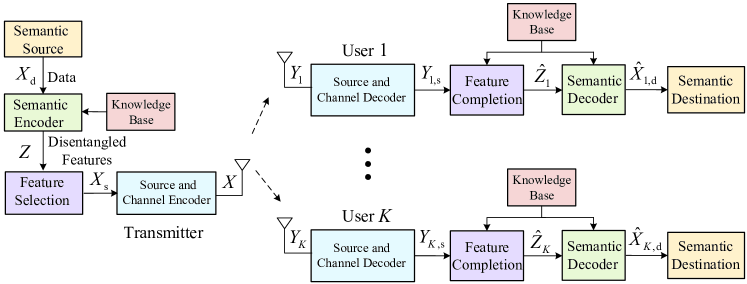
Figure 1: Features disentangled broadcast semantic communications framework

II Features Disentangled Semantic BC Framework

In order to design a practical semantic communication network, we propose a features-disentangled broadcast semantic BC framework, as shown in Fig. 1, which is compatible with existing 5G communication systems. Specifically, one semantic transmitter broadcasts the disentangled features to $K$ semantic users. The proposed semantic broadcast framework can simultaneously take advantage of the high transmission efficiency of semantic communications and the practical standards and hardware of 5G communications systems. In the following, we will introduce the modules of the proposed semantic broadcast framework in details.

II-1 Semantic Source

The semantic source produces original data ${X_{\rm{d}}}$, which generally includes both the intended semantic features and some unintended semantic features. Note that, each user may be interested in different features. Therefore, the semantic transmitter needs to send semantic features according to users’ interests, while the unintended semantic features do not need to be transmitted.

II-2 Semantic Encoder

Based on the knowledge base which involves shared knowledge between the transmitter and receivers, the semantic encoder extracts $L$ disentangled semantic features $Z={\left\{{{z_{l}}}\right\}_{l\in{\mathcal{L}}}}$ from the data ${{X_{\rm{d}}}}$, where ${z_{l}}$ denotes the $l$th semantic feature, and ${\mathcal{L}}\buildrel\Delta\over{=}\left\{{1,...,L}\right\}$. On one hand, the semantic encoder fulfills the function of a source encoder, which compresses the high-dimensional data ${{X_{\rm{d}}}}$ into low-dimensional semantic features $Z$. On the other hand, the semantic encoder also plays the role of channel encoder, which involves redundancy to combat the channel variations. Note that the redundancy added in the semantic encoder is to improve the robustness of transmission in the semantic level, while the conventional channel encoder improves the robustness at the bit level.

II-3 Features Selection

The disentangled semantic features $Z$ could contain multiple semantic features for multiple users, and users’ interested semantic features may be different. Therefore, the features selection module selects the semantic features for each user based on the task’s requirement. Specifically, let ${\{{z_{l}}\}_{l\in{{\mathcal{L}_{i}}}}}$ denote the interested features of User $i$, where ${{{\mathcal{L}}_{i}}}\subseteq{\mathcal{L}}$. Since User $i$ is only interested in the features ${\{{z_{l}}\}_{l\in{{\mathcal{L}_{i}}}}}$, the rest of the features $\{{z_{n}}\}_{n\in{\mathcal{L}\backslash{{\mathcal{L}_{i}}}}}$ can be viewed as the “redundancy” for User $i$. Then, let ${X_{i,{\rm{s}}}}$ denote the selected semantic features of User $i$, which is given as

$${X_{i,{\rm{s}}}}={\left\{{{z_{l}}}\right\}_{l\in{{\mathcal{L}_{i}}}}}.$$ (1)

Furthermore, the selected semantic features of $K$ users ${X_{\rm{s}}}$ are given as

$${X_{\rm{s}}}=\left\{{{X_{i,{\rm{s}}}}}\right\}_{i=1}^{K}.$$ (2)

At last, the selected semantic features ${X_{\rm{s}}}$ are encoded into $X$ through conventional bit-level source coding and channel coding, and then transmitted to the broadcast channel.

II-4 Semantic Broadcast Channel

For User $i$, the received signal $Y_{i}$ is decoded by the bit-level channel decoder and the source decoder, and output the estimated intended feature ${Y_{i,{\rm{s}}}}={\left\{{{{\widehat{z}}_{l}}}\right\}_{l\in{{\cal L}_{{{i}}}}}}$. The semantic broadcast channel with input $X_{s}$ and outputs $({Y_{1,{\rm{s}}}},\ldots,{Y_{K,{\rm{s}}}})$ can be characterized as the conditional probability

$$p\left({{Y_{1,s}},\ldots,{Y_{K,s}}|{X_{s}}}\right)\;{\mkern 1.0mu}= p\left({X|{X_{s}}}\right)P\left({{Y_{1}},\ldots,{Y_{K}}|X}\right)\prod\limits_{k=1}^{K}p\left({{Y_{k,{\rm{s}}}}|{Y_{k}}}\right),$$ (3)

where $P(Y_{1},\ldots,Y_{K}|X)$ is the transitional probability of the broadcast channel with $X$ being the channel input and $Y_{k}$ being the received signal at receiver $k$.

II-5 Feature Completion

Due to the feature selection, the unintended features are not transmitted, and the users only received the interested features. Consider the case that users aim to retrieve the source data based on the interested features. Then, a feature completion module can be used to help the users obtain the unintended features. Specifically, let ${\left\{{{{\overline{z}}_{t}}}\right\}_{l\in{\cal L}\backslash{{\cal L}_{i}}}}$ denote the unintended features obtained from the knowledge base. Based on ${\left\{{{{\overline{z}}_{t}}}\right\}_{l\in{\cal L}\backslash{{\cal L}_{i}}}}$ and the estimated interested features ${\left\{{{{\hat{z}}_{l}}}\right\}_{l\in{{\cal L}_{i}}}}$, User $i$ obtains the completed semantic features ${{\hat{Z}}_{i}}={\left\{{{{\hat{z}}_{l}}}\right\}_{l\in{{\cal L}_{i}}}}\cup{\left\{{{{\overline{z}}_{t}}}\right\}_{t\in{\cal L}\backslash{{\cal L}_{i}}}}$.

For example, considering a semantic BC system for staff clothing images transmission. The intended semantic features of each user may be different, i.e., some users may be interested in the staff’s hat features, while some users may be interested in the staff’s clothing features. There may be also some uninterested semantic features such as staff’s gender, skin color, and hairstyle, and background of the image. Therefore, the users can generate unintended semantic features based on the shared knowledge base, such as the staff’s gender, skin color and hairstyle. Note that, the generated unintended semantic features at the receiver may be different from the corresponding features of the image at the transmitter. Then, the user combines the received clothing features with its own generated unintended features. Moreover, both the simulation and prototype test verification of feature selection and completion will be presented in Table V.

II-6 Semantic Decoder and Semantic Destination

With the completed semantic features $\widehat{Z}_{i}$, the semantic decoder of User $i$ recovers the data ${\widehat{X}_{i,{\rm{d}}}}$ based on the knowledge base, and finally sends it to the semantic destination.

So far, the key modules of the proposed features-disentangled broadcast semantic BC framework have been introduced, and we will further present a feasible realization and prototype verification of this framework in Sections V and VI, respectively.

III Information-Theoretic Metrics of Semantic BCs

In this section, we further investigate two information-theoretic metrics for semantic BC: the ultimate compression rate under both the distortion and perception constraints [35], and the achievable rate region of the semantic BC. Specifically, we propose the optimal distortion allocation scheme for multi-source data semantic compression and derive the achievable rate region for the linear semantic BCs, where the conditional probability $p\left({{Y_{1,{\rm{s}}}},\ldots,{Y_{K,{\rm{s}}}}|{X_{\rm{s}}}}\right)$ satisfies the following relation

$${Y_{i,{\rm{s}}}}={G_{i}}{X_{\rm{s}}}+{N_{i,{\rm{s}}}},~{}i=1,...,K,$$ (4)

where ${G_{i}}$ denotes the effective channel gain of User $i$ from the feature selection module to the feature completion module, and ${N_{i,{\rm{s}}}}$ denotes the received semantic noise. Since the physical channel noise generally follows Gaussian distribution and the source encoder and channel encoder are non-linear mapping functions, the received semantic noise ${N_{i,{\rm{s}}}}$ is assumed to follow a non-Gaussian distribution with variance $\sigma_{i,{\rm{s}}}^{2}$.

III-A Distortion Allocation for Multi-Source Data Semantic Compression

Most of the existing semantic communications focused on a single source data semantic compression. However, in multi-user semantic BC networks, the interested data (or features) of each user may be different, and thus multi-source data compression is the general case in the multi-user semantic communication networks. The question naturally arises as to how we should allot this distortion to the multi-source data to minimize the total distortion under both the distortion and perception constraints.

Hence, we investigate the optimal distortion allocation scheme with ${L_{\rm{d}}}>1$ independent sources data ${\left\{{{X_{i{\rm{,d}}}}}\right\}_{i=1}^{L_{\rm{d}}}}$ for semantic BC networks. We aim to optimize distortion allocation for multi-source data compression with both squared error distortion and the perception constraints. Mathematically, the distortion allocation optimization can be formulated as

$$R\left({D,P}\right)=\mathop{\min}\limits_{\left\{{p\left({{{\widehat{X}}_{i{\rm{,d}}}}|{X_{i{\rm{,d}}}}}\right)}\right\}}~{} {\rm{I}}\left({\left\{{{X_{i{\rm{,d}}}}}\right\}_{i=1}^{L_{\rm{d}}};\left\{{{{\widehat{X}}_{i{\rm{,d}}}}}\right\}_{i=1}^{L_{\rm{d}}}}\right)$$ (5a)

$${\rm{s.t.}}~{} \sum\limits_{i=1}^{L_{\rm{d}}}{{\rm{E}}\left\{{{{\left\|{{X_{i{\rm{,d}}}}-{{\widehat{X}}_{i{\rm{,d}}}}}\right\|}^{2}}}\right\}}\leq D,$$ (5b)

$$\sum\limits_{i=1}^{L_{\rm{d}}}{{d_{{\rm{KL}}}^{\left(i\right)}}\left({{p_{{{\hat{X}}_{i,{\rm{d}}}}}},{p_{{X_{i,{\rm{d}}}}}}}\right)}\leq P,$$ (5c)

where $D$ and $P$ denote the total distortion and Kullback-Leibler (KL) divergence thresholds, respectively.

In this paper, we consider the multiple independent Gaussian distributed data ${\left\{{{X_{i{\rm{,d}}}}}\right\}_{i=1}^{L_{\rm{d}}}}$, i.e., ${X_{i,{\rm{d}}}}\sim\mathcal{N}\left({0,\sigma_{i,{\rm{d}}}^{2}}\right)$. Moreover, let ${{D}_{i}}$ denote the squared-error distortion between ${X_{i,{\rm{d}}}}$ and ${{\hat{X}}_{i,{\rm{d}}}}$, i.e.,

$${{D}_{i}}={\rm{E}}\left\{{{{\left\|{{X_{i,{\rm{d}}}}-{{\hat{X}}_{i,{\rm{d}}}}}\right\|}^{2}}}\right\}.$$ (6)

Then, the mutual information ${\rm{I}}\left({\left\{{{X_{i{\rm{,d}}}}}\right\}_{i=1}^{L_{\rm{d}}};\left\{{{{\widehat{X}}_{i{\rm{,d}}}}}\right\}_{i=1}^{L_{\rm{d}}}}\right)$ can be written as [37]

$${\rm{I}}\left({\left\{{{X_{i,{\rm{d}}}}}\right\}_{i=1}^{{L_{\rm{d}}}};\left\{{{{\hat{X}}_{i,{\rm{d}}}}}\right\}_{i=1}^{{L_{\rm{d}}}}}\right)=\sum\limits_{i=1}^{{L_{\rm{d}}}}{{{\left[{\frac{1}{2}\log\left({\frac{{\sigma_{i,{\rm{d}}}^{2}}}{{{D_{i}}}}}\right)}\right]}^{+}}},$$ (7)

where ${\widehat{X}_{i,{\rm{d}}}}$ follows a Gaussian distribution, i.e., ${\widehat{X}_{i,{\rm{d}}}}\sim\mathcal{N}\left({0,\sigma_{i{\rm{,d}}}^{2}-{D_{i}}}\right)$, and ${\left[x\right]^{+}}=x$ if $x\geq 0$, otherwise, ${\left[x\right]^{+}}=0$.

Thus, for the Gaussian distributed data ${X_{i,{\rm{d}}}}$ and the reconstructed data ${\widehat{X}_{i,{\rm{d}}}}$, the KL-divergence ${d_{{\rm{KL}}}^{\left(i\right)}}\left({{p_{{X_{i{\rm{,d}}}}}},{p_{{{\widehat{X}}_{i{\rm{,d}}}}}}}\right)$ is given as

$${d_{{\rm{KL}}}^{\left(i\right)}}\left({{p_{{{\hat{X}}_{i,{\rm{d}}}}}},{p_{{X_{i,{\rm{d}}}}}}}\right)=\frac{1}{2}\left({\ln\frac{{\sigma_{i,{\rm{d}}}^{2}}}{{\sigma_{i,{\rm{d}}}^{2}-{D_{i}}}}+\frac{{\sigma_{i,{\rm{d}}}^{2}-{D_{i}}}}{{\sigma_{i,{\rm{d}}}^{2}}}-1}\right).$$ (8)

Thus, the optimal distortion allocation problem (5) can be reformulated as

$$R\left({D,P}\right)=\mathop{\min}\limits_{\left\{{{D_{i}}}\right\}_{i=1}^{{L_{\rm{d}}}}} \sum\limits_{i=1}^{{L_{\rm{d}}}}{{{\left[{\frac{1}{2}\log\left({\frac{{\sigma_{i,{\rm{d}}}^{2}}}{{{D_{i}}}}}\right)}\right]}^{+}}}$$ (9a)

$${\rm{s}}.{\rm{t}}. \sum\limits_{i=1}^{L_{\rm{d}}}{{D_{i}}}\leq D,$$ (9b)

$$\sum\limits_{i=1}^{L_{\rm{d}}}{\frac{1}{2}\left({\ln\frac{{\sigma_{i,{\rm{d}}}^{2}}}{{\sigma_{i,{\rm{d}}}^{2}-{D_{i}}}}+\frac{{\sigma_{i,{\rm{d}}}^{2}-{D_{i}}}}{{\sigma_{i,{\rm{d}}}^{2}}}-1}\right)}\leq P.$$ (9c)

Note that, problem (9) is convex in $\left\{{{{{D}}_{i}}}\right\}$, and the Lagrangian function of problem (9) $L\left({\left\{{{D_{i}}}\right\},{\lambda_{D}},{\lambda_{P}}}\right)$ is given as

$$L\left({\left\{{{D_{i}}}\right\},{\lambda_{D}},{\lambda_{P}}}\right)= \sum\limits_{i=1}^{L_{\rm{d}}}{\frac{1}{2}\ln\frac{{{\sigma_{i,{\rm{d}}}^{2}}}}{{{D_{i}}}}+{\lambda_{D}}}\left({\sum\limits_{i=1}^{L_{\rm{d}}}{{D_{i}}}-D}\right)$$

$$+{\lambda_{P}}\left({\frac{1}{2}\sum\limits_{i=1}^{L_{\rm{d}}}{\left({\ln\frac{{{\sigma_{i,{\rm{d}}}^{2}}-{D_{i}}}}{{{\sigma_{i,{\rm{d}}}^{2}}}}+\frac{{{\sigma_{i,{\rm{d}}}^{2}}}}{{{\sigma_{i,{\rm{d}}}^{2}}-{D_{i}}}}-1}\right)}-P}\right),$$ (10)

where ${\lambda_{D}}\geq 0$ and ${\lambda_{P}}\geq 0$ are Lagrange multipliers associated with constraints (9b) and (9c), respectively.

Furthermore, let the first derivative of the function $L\left({\left\{{{D_{i}}}\right\},{\lambda_{D}},{\lambda_{P}}}\right)$ with respect to ${D_{i}}$ be equal to 0, i.e.,

$${-\frac{1}{{2{D_{i}}}}+{\lambda_{D}}+{\lambda_{P}}\frac{1}{2}\frac{{{D_{i}}}}{{{\sigma_{i,{\rm{d}}}^{2}}\left({{\sigma_{i,{\rm{d}}}^{2}}-{D_{i}}}\right)}}=0,~{}i=1,..,{L_{\rm{d}}}}.$$ (11)

Thus, the optimal distortions ${D_{i}}$ are given as

$${D_{i}}=\frac{{{\sigma_{i,{\rm{d}}}^{2}}\left({\sqrt{{{\left({1-2{\lambda_{D}}{\sigma_{i,{\rm{d}}}^{2}}}\right)}^{2}}+4{\lambda_{P}}}-\left({1+2{\lambda_{D}}{\sigma_{i,{\rm{d}}}^{2}}}\right)}\right)}}{{2\left({{\lambda_{P}}-2{\lambda_{D}}{\sigma_{i,{\rm{d}}}^{2}}}\right)}},$$ (12)

where the parameters $\lambda_{D}$ and $\lambda_{P}$ are the solutions of the following equations

$${{\lambda_{D}}\left({\sum\limits_{i=1}^{K}{{D_{i}}}-D}\right)=0},$$ (13a)

$${{\lambda_{P}}\left({\frac{1}{2}\sum\limits_{i=1}^{L_{\rm{d}}}{\left({\ln\frac{{{\sigma_{i,{\rm{d}}}^{2}}-{D_{i}}}}{{{\sigma_{i,{\rm{d}}}^{2}}}}+\frac{{{\sigma_{i,{\rm{d}}}^{2}}}}{{{\sigma_{i,{\rm{d}}}^{2}}-{D_{i}}}}-1}\right)}-P}\right)=0.}$$ (13b)

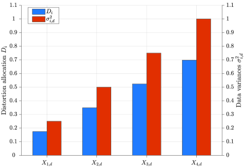
Figure 2: Distortion allocation for Gaussian distributed data $\left\{{{{\rm{X}}_{i,{\rm{d}}}}}\right\}_{i=1}^{4}$ with variances $\sigma_{1,{\rm{d}}}^{2}=0.25$, $\sigma_{i,{\rm{d}}}^{2}=0.5$, $\sigma_{i,{\rm{d}}}^{2}=0.75$,and $\sigma_{i,{\rm{d}}}^{2}=1$, respectively.

Thus, the rate distortion function of the data ${X_{i,{\rm{d}}}}$ is given as

$${R_{i}}={\left[{\frac{1}{2}\ln\frac{{2\left({{\lambda_{P}}-2{\lambda_{D}}\sigma_{i,{\rm{d}}}^{2}}\right)}}{{\sqrt{{{\left({1-2{\lambda_{D}}\sigma_{i,{\rm{d}}}^{2}}\right)}^{2}}+4{\lambda_{P}}}-\left({1+2{\lambda_{D}}\sigma_{i,{\rm{d}}}^{2}}\right)}}}\right]^{+}},$$ (14)

where $i=1,..,{L_{\rm{d}}}$. Fig. 2 shows the optimal distortion allocation for Gaussian distributed data $\left\{{{{\rm{X}}_{i,{\rm{d}}}}}\right\}_{i=1}^{4}$ with variances $\sigma_{1,{\rm{d}}}^{2}=0.25$, $\sigma_{i,{\rm{d}}}^{2}=0.5$, $\sigma_{i,{\rm{d}}}^{2}=0.75$, and $\sigma_{i,{\rm{d}}}^{2}=1$, respectively. From Fig. 2, we observe that with a larger data variance $\sigma_{i,{\rm{d}}}^{2}$, e.g., N = 50, the allocated distortion is more, i.e., the allocated distortion increases with the values of variance of the data.

III-B Achievable Rate Region of 2-Receiver Semantic Broadcast Channel

Due to the non-Gaussian distributed semantic channel noise, the classical Shannon capacity region results of the broadcast channel (based on Gaussian distributed noise) cannot directly be applied in semantic broadcast channels.

In the following, we establish an achievable rate region of the 2-user degraded semantic BCs with $|{G_{1}}|\geq|{G_{2}}|$ and $\sigma_{1,s}=\sigma_{2,s}$, which implies that User 2 observes stronger signals than that of User 1. The main idea is that the broadcast transmitter employs semantic features splitting and superposition, and users employ successive interference cancelation (SIC)[37]. Specifically, since ${G_{1}}>{G_{2}}$, the semantic feature ${X_{{\rm{2}},{\rm{s}}}}$ for user $2$, which can be viewed as common message, is encoded into the cloud center signal, while the semantic feature ${X_{{\rm{1}},{\rm{s}}}}$, which can be viewed as private message, is encoded into the satellite signal. Let ${R_{1,{\rm{s}}}}$ and ${R_{2,{\rm{s}}}}$ denote the information rates from the feature selection module of the transmitter to the feature completion module of Users $1$ and $2$, respectively. A rate pair $\left({{{R_{1,{\rm{s}}}}},{{R_{2,{\rm{s}}}}}}\right)$ is achievable for the 2-user degraded semantic BCs if it satisfies the conditions [37]

$${R_{1,{\rm{s}}}}\leq{\rm{I}}\left({{X_{{\rm{1,s}}}};{Y_{1{\rm{,s}}}}|{X_{{\rm{2,s}}}}}\right),$$ (15a)

$${R_{2,{\rm{s}}}}\leq{\rm{I}}\left({{X_{{\rm{2,s}}}};{Y_{2{\rm{,s}}}}}\right).$$ (15b)

Moreover, let $P$ denote the total transmission power of the transmitter, and ${\alpha}P$ and ${\left({1-\alpha}\right)P}$ denote the allocated power to the semantic feature ${X_{{\rm{1}},{\rm{s}}}}$ and ${\left({1-\alpha}\right)P}$, respectively, where ${\alpha}\in\left[{0,1}\right]$ is a power allocation factor. Thus, the transmitted signal $X$ of the semantic broadcast network is given as

$$X=\sqrt{\alpha P}{X_{{\rm{1}},{\rm{s}}}}+\sqrt{\left({1-\alpha}\right)P}{X_{{\rm{2}},{\rm{s}}}}.$$ (16)

The received signals at User $1$ and User $2$ are, respectively, given as

$${Y_{{\rm{1}},{\rm{s}}}}={G_{1}}\sqrt{\alpha P}{X_{{\rm{1}},{\rm{s}}}}+{G_{1}}\sqrt{\left({1-\alpha}\right)P}{X_{{\rm{2}},{\rm{s}}}}+{N_{{\rm{1}},{\rm{s}}}},$$ (17a)

$${Y_{2,{\rm{s}}}}={G_{2}}\sqrt{\alpha P}{X_{{\rm{1}},{\rm{s}}}}+{G_{2}}\sqrt{\left({1-\alpha}\right)P}{X_{{\rm{2}},{\rm{s}}}}+{N_{{\rm{2}},{\rm{s}}}}.$$ (17b)

User $1$ utilizes SIC to decode the semantic feature ${X_{{\rm{2}},{\rm{s}}}}$ first and cancel ${X_{{\rm{2}},{\rm{s}}}}$ from the received signal. Then, User $1$ decodes the semantic feature ${X_{{\rm{1}},{\rm{s}}}}$. After SIC, the residual received signal of User $1$ is given as

$$Y_{{\rm{1}},{\rm{s}}}^{{\rm{SIC}}}={G_{1}}\sqrt{{\alpha}P}{X_{{\rm{1}},{\rm{s}}}}+{N_{{\rm{1}},{\rm{s}}}}$$ (18)

While User $2$ can only decode the semantic feature ${X_{{\rm{2}},{\rm{s}}}}$, and the semantic feature ${X_{{\rm{1}},{\rm{s}}}}$ is the interference for user $2$.

Lemma 1 (Achievable rate region of degraded semantic broadcast channels).

Consider the degraded semantic broadcast channel, where ${G_{1}}>{G_{2}}$, the achievable rates ${R_{1,{\rm{s}}}}$ and ${R_{2,{\rm{s}}}}$ are bounded by

$$R_{{\rm{1}},{\rm{s}}}^{{\rm{eq}}}\leq{R_{1,{\rm{s}}}}\leq R_{{\rm{1}},{\rm{s}}}^{{\rm{eq}}}+{d_{{\rm{KL}}}}\left({{p_{{N_{{\rm{1}},{\rm{s}}}}}}\left(x\right),{p_{N_{{\rm{1}},{\rm{s}}}^{{\rm{eq}}}}}\left(x\right)}\right),$$ (19a)

$$R_{2,{\rm{s}}}^{{\rm{eq}}}\leq{R_{2,{\rm{s}}}}\leq R_{2,{\rm{s}}}^{{\rm{eq}}}+{d_{{\rm{KL}}}}\left({{p_{{N_{2,{\rm{s}}}}}}\left(x\right),{p_{N_{2,{\rm{s}}}^{{\rm{eq}}}}}\left(x\right)}\right),$$ (19b)

where $N_{1,{\rm{s}}}^{{\rm{eq}}}$ and $N_{2,{\rm{s}}}^{{\rm{eq}}}$ are the equivalent Gaussian distributed noises with the same variances as ${N_{{\rm{1}},{\rm{s}}}}$ and ${N_{{\rm{1}},{\rm{s}}}}$, respectively, i.e., ${\mathop{\rm var}}\left({N_{1,{\rm{s}}}^{{\rm{eq}}}}\right)=\sigma_{1,{\rm{s}}}^{2}$, and ${\mathop{\rm var}}\left({N_{2,{\rm{s}}}^{{\rm{eq}}}}\right)=\sigma_{2,{\rm{s}}}^{2}$, ${d_{{\rm{KL}}}}\left({p\left(x\right),q\left(x\right)}\right)=\int_{-\infty}^{\infty}{p\left(x\right)\log\frac{{p\left(x\right)}}{{q\left(x\right)}}}{\rm{d}}x$, and

$$R_{{\rm{1}},{\rm{s}}}^{{\rm{eq}}}=\frac{1}{2}{\log_{2}}\left({1+\frac{{G_{1}^{2}{\alpha_{1}}P}}{{\sigma_{1,s}^{2}}}}\right),$$ (20a)

$$R_{{\rm{2}},{\rm{s}}}^{{\rm{eq}}}=\frac{1}{2}{\log_{2}}\left({1+\frac{{G_{2}^{2}\left({1-\alpha}\right)P}}{{G_{2}^{2}{\alpha_{1}}P+\sigma_{2,s}^{2}}}}\right).$$ (20b)

Proof: We first introduce the equivalent Gaussian distributed channel noises $N_{1,{\rm{s}}}^{{\rm{eq}}}$ and $N_{2,{\rm{s}}}^{{\rm{eq}}}$ with the same variances as ${N_{{\rm{1}},{\rm{s}}}}$ and ${N_{{{2}},{\rm{s}}}}$, respectively, i.e., ${\mathop{\rm var}}\left({N_{1,{\rm{s}}}^{{\rm{eq}}}}\right)=\sigma_{1,{\rm{s}}}^{2}$, and ${\mathop{\rm var}}\left({N_{2,{\rm{s}}}^{{\rm{eq}}}}\right)=\sigma_{2,{\rm{s}}}^{2}$. The PDFs of $N_{1,{\rm{s}}}^{{\rm{eq}}}$ and $N_{2,{\rm{s}}}^{{\rm{eq}}}$ are, respectively, given as

$${p_{N_{1,{\rm{s}}}^{{\rm{eq}}}}}\left(x\right)=\frac{1}{{\sqrt{\pi}{\sigma_{1,s}}}}\exp\left({-\frac{{{x^{2}}}}{{\sigma_{1,s}^{2}}}}\right),$$ (21a)

$${p_{N_{2,{\rm{s}}}^{{\rm{eq}}}}}\left(x\right)=\frac{1}{{\sqrt{\pi}{\sigma_{2,s}}}}\exp\left({-\frac{{{x^{2}}}}{{\sigma_{2,s}^{2}}}}\right).$$ (21b)

With the equivalent Gaussian distributed channel noise $N_{1,{\rm{s}}}^{{\rm{eq}}}$ and $N_{2,{\rm{s}}}^{{\rm{eq}}}$, the corresponding rates of User $1$ and User $2$ are, respectively, given as

$$R_{{\rm{1}},{\rm{s}}}^{{\rm{eq}}}=\frac{1}{2}{\log_{2}}\left({1+\frac{{G_{1}^{2}{\alpha_{1}}P}}{{\sigma_{1,s}^{2}}}}\right),$$ (22a)

$$R_{{\rm{2}},{\rm{s}}}^{{\rm{eq}}}=\frac{1}{2}{\log_{2}}\left({1+\frac{{G_{2}^{2}\left({1-\alpha}\right)P}}{{G_{2}^{2}{\alpha_{1}}P+\sigma_{2,s}^{2}}}}\right).$$ (22b)

For the non-Gaussian distributed channel noise ${N_{{{1}},{\rm{s}}}}$ and ${N_{{{2}},{\rm{s}}}}$, the semantic communication rates $R_{1}$ and $R_{2}$ are bounded by [38]

$$R_{{\rm{1}},{\rm{s}}}^{{\rm{eq}}}\leq{R_{1,{\rm{s}}}}\leq R_{{{1}},{\rm{s}}}^{{\rm{eq}}}+{d_{{\rm{KL}}}}\left({{p_{{N_{{{1}},{\rm{s}}}}}}\left(x\right),{p_{N_{{{1}},{\rm{s}}}^{{\rm{eq}}}}}\left(x\right)}\right),$$ (23a)

$$R_{2,{\rm{s}}}^{{\rm{eq}}}\leq{R_{2,{\rm{s}}}}\leq R_{2,{\rm{s}}}^{{\rm{eq}}}+{d_{{\rm{KL}}}}\left({{p_{{N_{2,{\rm{s}}}}}}\left(x\right),{p_{N_{2,{\rm{s}}}^{{\rm{eq}}}}}\left(x\right)}\right).$$ (23b)

∎

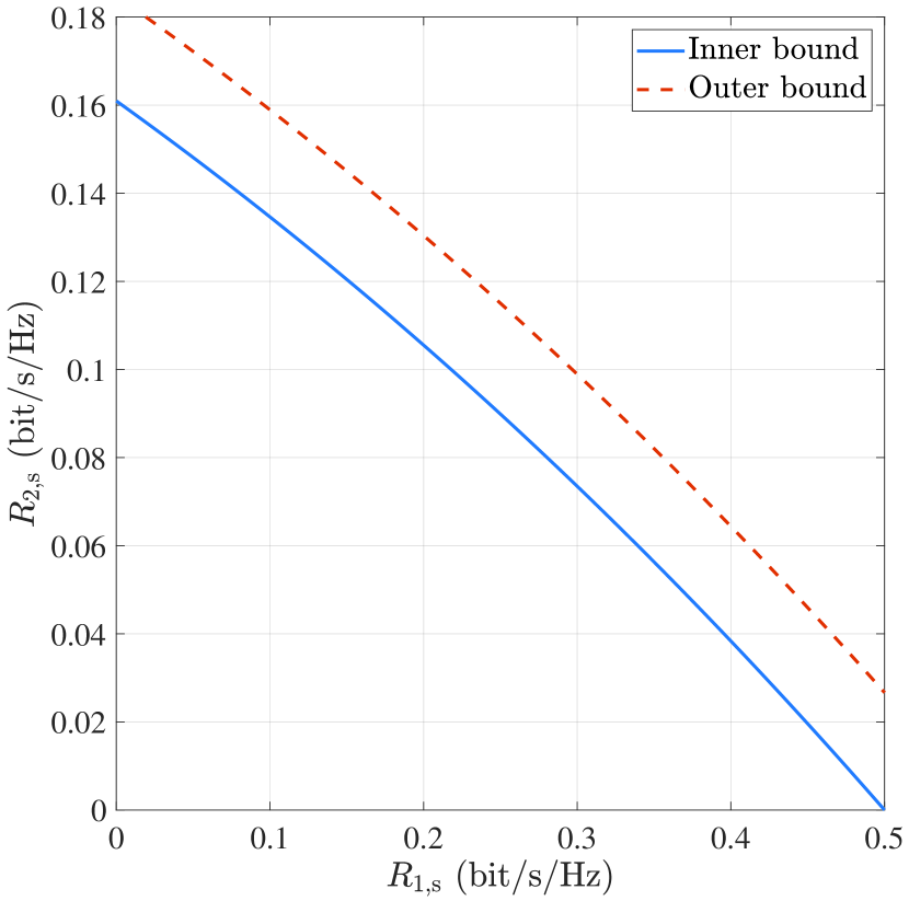
(a)

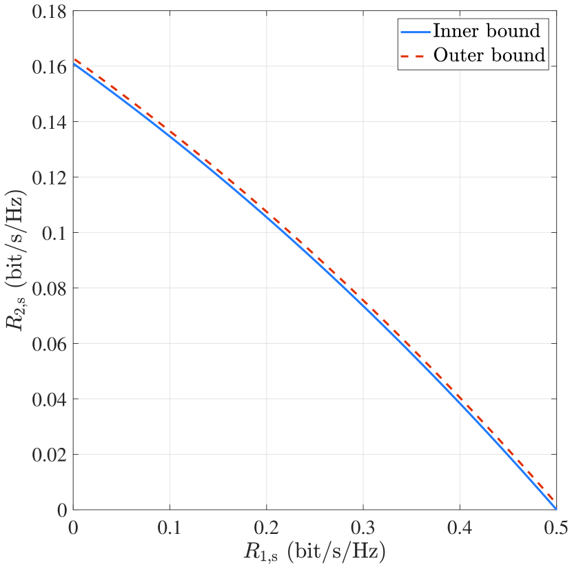
(b)

Figure 3: (a) Inner and outer bounds of semantic broadcast rate region with ${p_{{N_{{\rm{1}},{\rm{s}}}}}}\left(x\right)={p_{{N_{2,{\rm{s}}}}}}\left(x\right)={q_{1}}\left(x\right)$; (b) Inner and outer bounds of semantic broadcast rate region with ${p_{{N_{{\rm{1}},{\rm{s}}}}}}\left(x\right)={p_{{N_{2,{\rm{s}}}}}}\left(x\right)={q_{2}}\left(x\right)$.

In the following, we numerically demonstrate the derived achievable rates region results (19) of the semantic broadcast channel with two different PDFs ${q_{1}}\left(x\right)$ and ${q_{2}}\left(x\right)$ cases with the same variances, i.e., ${q_{1}}\left(x\right)\buildrel\Delta\over{=}\frac{1}{{2\sqrt{3}}}\left({{\rm{erf}}\left({\frac{1}{{\sqrt{2}}}-\sqrt{\frac{2}{3}}x}\right)+{\rm{erf}}\left({\frac{1}{{\sqrt{2}}}+\sqrt{\frac{2}{3}}x}\right)}\right)$ and ${q_{2}}\left(x\right)\buildrel\Delta\over{=}\frac{1}{{2\sqrt{3}}}\left({{\rm{erf}}\left({\frac{{3\sqrt{2}}}{5}-\sqrt{\frac{2}{3}}x}\right)+{\rm{erf}}\left({\frac{{3\sqrt{2}}}{5}+\sqrt{\frac{2}{3}}x}\right)}\right)$. Fig. 3 (a) and (b) depict the inner and outer bounds of the semantic broadcast rate region with ${p_{{N_{{\rm{1}},{\rm{s}}}}}}\left(x\right)={p_{{N_{2,{\rm{s}}}}}}\left(x\right)={q_{1}}\left(x\right)$ and ${p_{{N_{{\rm{1}},{\rm{s}}}}}}\left(x\right)={p_{{N_{2,{\rm{s}}}}}}\left(x\right)={q_{2}}\left(x\right)$ respectively, where ${{{G}}_{1}}=1$ and ${{{G}}_{2}}=0.5$. Comparing Fig. 3 (a) and (b), it can be observed that the gap between the inner bound and outer bound is significantly tighter in Fig. 3 (b). The reason is that the KL ${d_{{\rm{KL}}}}\left({{p_{{N_{{\rm{1}},{\rm{s}}}}}}\left(x\right),{p_{N_{{\rm{1}},{\rm{s}}}^{{\rm{eq}}}}}\left(x\right)}\right)$ is smaller than that in Fig. 3 (a) case, i.e., the distributions ${p_{{N_{{\rm{1}},{\rm{s}}}}}}\left(x\right)={p_{{N_{2,{\rm{s}}}}}}\left(x\right)={q_{2}}\left(x\right)$ are closer to the Gaussian distribution than ${p_{{N_{{\rm{1}},{\rm{s}}}}}}\left(x\right)={p_{{N_{2,{\rm{s}}}}}}\left(x\right)={q_{1}}\left(x\right)$. Moreover, when the KL divergence tends to $0$, i.e., ${d_{{\rm{KL}}}}\left({{p_{{N_{{\rm{1}},{\rm{s}}}}}}\left(x\right),{p_{N_{{\rm{1}},{\rm{s}}}^{{\rm{eq}}}}}\left(x\right)}\right)\to 0$, the gap between the inner bound and the upper bound in (19) tends to 0.

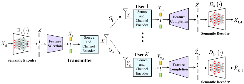
Figure 4: Proposed features-disentangled semantic BC network

Note that, although we have derived two information theoretic metrics for semantic BC, based on some strong prior information, these derivations are based on some strong prior information, such as the probability distribution of the semantic information is assumed known, and the verification of these theories will be explored in the future.

IV Features Disentangled Semantic BC System Design

IV-A Supervised AE Based Semantic Broadcast System Design

Based on the proposed semantic broadcast framework in Fig. 2, we propose a features-disentangled semantic BC network design, as shown in Fig. 4, which includes a single semantic encoder ${{\rm{E}}_{\phi}}\left(\cdot\right)$ with parameters set $\phi$, and $K$ semantic decoders $\left\{{{{\rm{D}}_{{\theta_{i}}}}\left(\cdot\right)}\right\}_{i=1}^{K}$ with parameters sets $\left\{{{\theta_{i}}}\right\}_{i=1}^{K}$. More specifically, the transmitter with the encoder network ${{\rm{E}}_{\phi}}\left(\cdot\right)$ extracts the semantic features from the source data and disentangles them into multiple independent and interpretable semantic features. Then, by applying semantic features selection, the transmitter broadcasts the semantic features to the intended users. After receiving the intended semantic features, User $i$ completes the unintended features with the help of the knowledge base, and decodes the semantic features with the decoder network ${{\rm{D}}_{{\theta_{i}}}}\left(\cdot\right)$, where $i=1,...,K$.

Specifically, to achieve controllable disentangled semantic features learning, we exploit the supervised AE to train the semantic broadcast network in three steps: self reconstruction, exchange common features, and exchange different features, which is motivated by the group-supervised learning strategy [36]. In the following, we will introduce the three training steps in details.

IV-A1 Self Reconstruction

As shown in Fig. 5 (a), the self reconstruction training can be regarded as a regular term to ensure that all the semantic information of the input data can be encoded into latent semantic features to avoid information loss. Specifically, the semantic encoder ${{\rm{E}}_{\phi}}$ compresses the $l$th data sample ${X_{\rm{d}}^{\left(l\right)}}$ into a latent semantic feature vector ${{\rm{Z}}^{\left(l\right)}}$, i.e.,

$${{\rm{Z}}^{\left(l\right)}}={{\rm{E}}_{\phi}}\left({X_{\rm{d}}^{\left(l\right)}}\right),$$ (24)

where $l=1,...,{L_{\rm{s}}}$, and ${L_{\rm{s}}}$ denotes the total amount of the sampled data.

Then, the semantic feature vector ${{\rm{Z}}^{\left(l\right)}}$ is broadcasted to $K$ semantic users. At the user end, the received semantic features of User $i$ are given as

$$\widehat{\rm{Z}}_{i}^{\left(l\right)}={G_{i}}{{\rm{Z}}^{\left(l\right)}}+{N_{i,{\rm{s}}}},~{}i=1,...,K.$$ (25)

Then, User $i$ decodes the received semantic features $\widehat{\rm{Z}}_{i}^{\left(l\right)}$ and obtains the reconstructed data $\widehat{X}_{i{\rm{,d}}}^{\left(l\right)}$ as follows

$$\widehat{X}_{i{\rm{,d}}}^{\left(l\right)}={{\rm{D}}_{{\theta_{i}}}}\left({\widehat{\rm{Z}}_{i}^{\left(l\right)}}\right),~{}i=1,...,K.$$ (26)

Finally, the semantic encoder ${{\rm{E}}_{\phi}}\left(\cdot\right)$ with parameters set $\phi$, and $K$ semantic decoders $\left\{{{{\rm{D}}_{{\theta_{i}}}}\left(\cdot\right)}\right\}_{i=1}^{K}$ with parameters sets $\left\{{{\theta_{i}}}\right\}_{i=1}^{K}$ are jointly optimized based on the standard AE reconstruction loss ${L_{{\rm{SAE,1}}}}$ as follows

$${L_{{\rm{AE}},{\rm{1}}}}=\sum\limits_{l=1}^{{L_{\rm{s}}}}{\sum\limits_{i=1}^{K}{{{\left\|{X_{\rm{d}}^{\left(l\right)}-\hat{X}_{i,{\rm{d}}}^{\left(l\right)}}\right\|}^{2}}}}.$$ (27)

IV-A2 Common Semantic Features Exchange

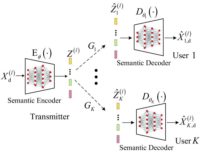
(a)

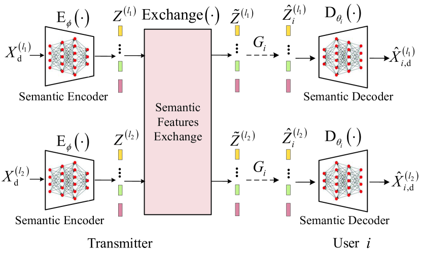
(b)

Figure 5: (a) Self reconstruction training; (b) Semantic features exchange training.

To improve the semantic features extraction ability of the network, we further train the proposed semantic broadcast network by exchanging the common semantic features, and minimize the reconstruction loss of the common semantic features exchange. As shown in Fig. 5 (b), we choose two input data samples ${X_{\rm{d}}^{\left({{l_{1}}}\right)}}$ and ${X_{\rm{d}}^{\left({{l_{2}}}\right)}}$ with common semantic features, and extract the semantic features ${{\rm{Z}}^{\left({{l_{1}}}\right)}}$ and ${{\rm{Z}}^{\left({{l_{2}}}\right)}}$ through the semantic encoder ${{\rm{E}}_{\phi}}$ as follows

$${{\rm{Z}}^{\left({{l_{1}}}\right)}}=\left[{{\rm{z}}_{1}^{\left({{l_{1}}}\right)},...,{\rm{z}}_{K}^{\left({{l_{1}}}\right)}}\right]={{\rm{E}}_{\phi}}\left({X_{\rm{d}}^{\left({{l_{1}}}\right)}}\right),$$ (28a)

$${{\rm{Z}}^{\left({{l_{2}}}\right)}}=\left[{{\rm{z}}_{1}^{\left({{l_{2}}}\right)},...,{\rm{z}}_{K}^{\left({{l_{2}}}\right)}}\right]={{\rm{E}}_{\phi}}\left({X_{\rm{d}}^{\left({{l_{2}}}\right)}}\right),$$ (28b)

where ${l_{1}},{l_{2}}=1,...,{L_{\rm{s}}}$. Assume that the $j$th semantic feature of ${{\rm{Z}}^{\left({{l_{1}}}\right)}}$ and ${{\rm{Z}}^{\left({{l_{2}}}\right)}}$ are the same, i.e., ${{\rm{z}}_{j}^{\left({{l_{1}}}\right)}}$ and ${{\rm{z}}_{j}^{\left({{l_{2}}}\right)}}$ share the common semantic feature. Then, we swap the $j$th semantic feature of ${{\rm{Z}}^{\left({{l_{1}}}\right)}}$ and ${{\rm{Z}}^{\left({{l_{2}}}\right)}}$ as follows

$$\left[\begin{array}[]{l}{\widetilde{\rm{Z}}^{\left({{l_{1}}}\right)}}\\ {\widetilde{\rm{Z}}^{\left({{l_{2}}}\right)}}\end{array}\right] ={\rm{Exchange}}\left({{{\rm{Z}}^{\left({{l_{1}}}\right)}},{{\rm{Z}}^{\left({{l_{2}}}\right)}},j}\right)$$ (29c)

$$=\left[\begin{array}[]{l}{\rm{z}}_{1}^{\left({{l_{1}}}\right)},...,{\rm{z}}_{j}^{\left({{l_{2}}}\right)},...,{\rm{z}}_{K}^{\left({{l_{1}}}\right)}\\ {\rm{z}}_{1}^{\left({{l_{2}}}\right)},...,{\rm{z}}_{j}^{\left({{l_{1}}}\right)},...,{\rm{z}}_{K}^{\left({{l_{2}}}\right)}\end{array}\right],$$ (29f)

where ${\widetilde{\rm{Z}}^{\left({{l_{1}}}\right)}}$ and ${\widetilde{\rm{Z}}^{\left({{l_{2}}}\right)}}$ represent the data samples after feature exchange of ${{\rm{Z}}^{\left({{l_{1}}}\right)}}$ and ${{\rm{Z}}^{\left({{l_{2}}}\right)}}$ respectively, $j=1,...,{L_{\rm{c}}}$, and ${L_{\rm{c}}}$ denotes the total number of the common semantic features. Then, the exchanged common semantic features ${\widetilde{\rm{Z}}^{\left({{l_{1}}}\right)}}$ and ${\widetilde{\rm{Z}}^{\left({{l_{2}}}\right)}}$ are broadcasted to the $K$ users. For User $i$, let $\widehat{\rm{Z}}_{i}^{\left({{l_{1}}}\right)}$ and $\widehat{\rm{Z}}_{i}^{\left({{l_{2}}}\right)}$, respectively, denote the received semantic features of ${\widetilde{\rm{Z}}^{\left({{l_{1}}}\right)}}$ and ${\widetilde{\rm{Z}}^{\left({{l_{2}}}\right)}}$, i.e.,

$$\widehat{\rm{Z}}_{i}^{\left({{l_{1}}}\right)}={{\rm{G}}_{i}}{\widetilde{\rm{Z}}^{\left({{l_{1}}}\right)}}+{N_{i,{\rm{s}}}},$$ (30a)

$$\widehat{\rm{Z}}_{i}^{\left({{l_{2}}}\right)}={G_{i}}{\widetilde{\rm{Z}}^{\left({{l_{2}}}\right)}}+{N_{i,{\rm{s}}}},$$ (30b)

where $i=1,...,K$. Furthermore, by leveraging the semantic decoder ${{\rm{D}}_{{\theta_{i}}}}\left(\cdot\right)$, the reconstructed data $\widehat{X}_{i{\rm{,d}}}^{\left({{l_{1}}}\right)}$ and $\widehat{X}_{i{\rm{,d}}}^{\left({{l_{2}}}\right)}$ are, respectively, given as

$$\widehat{X}_{i{\rm{,d}}}^{\left({{l_{1}}}\right)}={{\rm{D}}_{{\theta_{i}}}}\left({\widehat{\rm{Z}}_{i}^{\left({{l_{1}}}\right)}}\right),$$ (31a)

$$\widehat{X}_{i{\rm{,d}}}^{\left({{l_{2}}}\right)}={{\rm{D}}_{{\theta_{i}}}}\left({\widehat{\rm{Z}}_{i}^{\left({{l_{2}}}\right)}}\right).$$ (31b)

Finally, for the common semantic features exchange training, the reconstruction loss of the semantic broadcast network ${L_{{\rm{AE,2}}}}$ is given as

$${L_{{\rm{AE}},{\rm{2}}}}=\sum\limits_{i=1}^{K}{\sum\limits_{\scriptstyle{l_{1}},{l_{2}}=1,\hfill\atop\scriptstyle{l_{2}}\neq{l_{1}}\hfill}^{{L_{\rm{c}}}}{\left({{{\left\|{\hat{X}_{i,{\rm{d}}}^{\left({{l_{1}}}\right)}-X_{\rm{d}}^{\left({{l_{1}}}\right)}}\right\|}^{2}}+{{\left\|{\hat{X}_{i,{\rm{d}}}^{\left({{l_{2}}}\right)}-X_{\rm{d}}^{\left({{l_{2}}}\right)}}\right\|}^{2}}}\right)}}.$$

IV-A3 Different Semantic Features Exchange

In order to enhance the ability of decoupling different semantic features, we train the semantic BC network by exchanging the different semantic features, and minimizing the reconstruction loss of different semantic features exchanges. Specifically, as shown in Fig. 5 (b), we choose two input data samples ${X_{\rm{d}}^{\left({{l_{1}}}\right)}}$ and ${X_{\rm{d}}^{\left({{l_{3}}}\right)}}$ with different semantic features, and extract the semantic features ${{\rm{Z}}^{\left({{l_{1}}}\right)}}$ and ${{\rm{Z}}^{\left({{l_{3}}}\right)}}$ through the semantic encoder ${{\rm{E}}_{\phi}}$ as follows

$${{\rm{Z}}^{\left({{l_{1}}}\right)}}={{\rm{E}}_{\phi}}\left({X_{\rm{d}}^{\left({{l_{1}}}\right)}}\right),$$ (32a)

$${{\rm{Z}}^{\left({{l_{3}}}\right)}}={{\rm{E}}_{\phi}}\left({X_{\rm{d}}^{\left({{l_{3}}}\right)}},\right)$$ (32b)

where ${l_{1}},{l_{3}}=1,...,{L_{\rm{s}}}$. Assume that the $n$th semantic features of ${{\rm{Z}}^{\left({{l_{1}}}\right)}}$ and ${{\rm{Z}}^{\left({{l_{3}}}\right)}}$ are different, i.e., ${{\rm{z}}_{j}^{\left({{l_{1}}}\right)}}$ and ${{\rm{z}}_{n}^{\left({{l_{3}}}\right)}}$ are different. Then, we swap the $n$th semantic feature of ${{\rm{Z}}^{\left({{l_{1}}}\right)}}$ and ${{\rm{Z}}^{\left({{l_{3}}}\right)}}$ as follows

$$\left[\begin{array}[]{l}{\widetilde{\rm{Z}}^{\left({{l_{1}}}\right)}}\\ {\widetilde{\rm{Z}}^{\left({{l_{3}}}\right)}}\end{array}\right]={\rm{Exchange}}\left({{{\rm{Z}}^{\left({{l_{1}}}\right)}},{{\rm{Z}}^{\left({{l_{3}}}\right)}},n}\right).$$ (35)

where ${\widetilde{\rm{Z}}^{\left({{l_{1}}}\right)}}$ and ${\widetilde{\rm{Z}}^{\left({{l_{3}}}\right)}}$ represent the data samples after feature exchange of ${{\rm{Z}}^{\left({{l_{1}}}\right)}}$ and ${{\rm{Z}}^{\left({{l_{3}}}\right)}}$ respectively, $n=1,...,{L_{\rm{e}}}$, and ${L_{\rm{e}}}$ denotes the total number of the different semantic features.

Then, the exchanged semantic features ${\widetilde{\rm{Z}}^{\left({{l_{1}}}\right)}}$ and ${\widetilde{\rm{Z}}^{\left({{l_{3}}}\right)}}$ are, respectively, broadcasted to the $K$ users. For User $i$, let $\widetilde{\rm{Z}}_{i,{\rm{r}}}^{\left({{l_{1}}}\right)}$ and $\widetilde{\rm{Z}}_{i,{\rm{r}}}^{\left({{l_{3}}}\right)}$, respectively, denote the received semantic features of ${\widetilde{\rm{Z}}^{\left({{l_{1}}}\right)}}$ and ${\widetilde{\rm{Z}}^{\left({{l_{3}}}\right)}}$, i.e.,

$$\widetilde{\rm{Z}}_{i,{\rm{r}}}^{\left({{l_{1}}}\right)}={\alpha_{i}}{\widetilde{\rm{Z}}^{\left({{l_{1}}}\right)}}+{N_{i,{\rm{s}}}},$$ (36a)

$$\widetilde{\rm{Z}}_{i,{\rm{r}}}^{\left({{l_{3}}}\right)}={\alpha_{i}}{\widetilde{\rm{Z}}^{\left({{l_{3}}}\right)}}+{N_{i,{\rm{s}}}},$$ (36b)

where $i=1,...,K$. Furthermore, based the semantic decoder ${{\rm{D}}_{{\theta_{i}}}}\left(\cdot\right)$, the reconstructed data $\widetilde{X}_{i,{\rm{d}}}^{\left({{l_{1}}}\right)}$ and $\widetilde{X}_{i,{\rm{d}}}^{\left({{l_{3}}}\right)}$ of User $i$ are given as

$$\widetilde{X}_{i,{\rm{d}}}^{\left({{l_{1}}}\right)}={{\rm{D}}_{{\theta_{i}}}}\left({\widetilde{\rm{Z}}_{i,{\rm{r}}}^{\left({{l_{1}}}\right)}}\right),$$ (37a)

$$\widetilde{X}_{i,{\rm{d}}}^{\left({{l_{3}}}\right)}={{\rm{D}}_{{\theta_{i}}}}\left({\widetilde{\rm{Z}}_{i,{\rm{r}}}^{\left({{l_{1}}}\right)}}\right).$$ (37b)

Then, by taking the reconstructed samples $\widehat{X}_{i{\rm{,d}}}^{\left({{l_{1}}}\right)}$ and $\widehat{X}_{i{\rm{,d}}}^{\left({{l_{3}}}\right)}$ as input data samples, the semantic broadcast network repeats the semantic encoding in (32), different semantic features exchange in (35), broadcasting the semantic features in (36) and decoding semantic features in (37). For brevity, we omit the details. Note that, both semantic feature exchange the $n$th feature. Hence, after two semantic feature exchanges, the different features exchanged each return to their original data samples.

After two semantic features exchanges, let ${\overline{X}_{i,{\rm{d}}}^{\left({{l_{1}}}\right)}}$ and ${\overline{X}_{i,{\rm{d}}}^{\left({{l_{3}}}\right)}}$ denote the final reconstructed data, respectively, and the corresponding reconstruction loss ${L_{{\rm{AE,3}}}}$ is given as

$${L_{{\rm{AE}},{\rm{3}}}}=\sum\limits_{i=1}^{K}{\sum\limits_{\scriptstyle{l_{1}},{l_{3}}=1,\hfill\atop\scriptstyle{l_{3}}\neq{l_{1}}\hfill}^{{L_{\rm{e}}}}{\left({{{\left\|{\overline{X}_{i,{\rm{d}}}^{\left({{l_{1}}}\right)}-X_{\rm{d}}^{\left({{l_{1}}}\right)}}\right\|}^{2}}+{{\left\|{\overline{X}_{i,{\rm{d}}}^{\left({{l_{3}}}\right)}-X_{\rm{d}}^{\left({{l_{3}}}\right)}}\right\|}^{2}}}\right)}}.$$

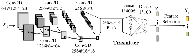
(a)

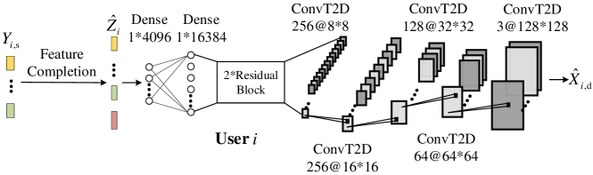
(b)

Figure 6: (a) The semantic transmitter architecture ; (b) Semantic User $i$.

IV-B Proposed Semantic BC Network Architecture

The proposed semantic broadcast network architecture includes a semantic transmitter network and $K$ semantic users network, as shown in Fig. 6, where the notation Conv2D 64$@$64*64 means that the network has 64 2-D convolutional filters with output size 64*64, Dense 1*4096 represents a dense layer with 4096 neurons, and Residual Block represents a convolution block with Conv2D 256$@$8*8 $\to$ Conv2D 256$@$8*8. More specifically, the details of the proposed semantic broadcast network architecture are listed as follows:

IV-B1 The network architecture of the transmitter

${X_{\rm{d}}}$ $\to$ Conv2D 64$@$128*128 $\to$ Conv2D 128$@$64*64 $\to$ Conv2D 256$@$32*32 $\to$ Conv2D 256$@$16*16 $\to$ Conv2D 256$@$8*8 $\to$ 2*Residual Block $\to$ Dense 1*4096 $\to$ Dense 1*100 $\to$ $\left\{{{z_{l}}}\right\}_{l=1}^{100}$ $\to$ ${X_{\rm{s}}}$;

IV-B2 The network architecture of User $i$

${Y_{i,{\rm{d}}}}$ $\to$ $\left\{{{{\widehat{z}}_{l}}}\right\}_{l=1}^{100}$ $\to$ Dense 1*4096 $\to$ Dense 1*16384 $\to$ 2*Residual Block $\to$ ConvT2D 256$@$8*8 $\to$ ConvT2D 256$@$16*16 $\to$ ConvT2D 128$@$32*32 $\to$ ConvT2D 64$@$64*64 $\to$ ConvT2D 3$@$128*128 $\to$ ${\widehat{X}_{i,{\rm{d}}}}$.

V Semantic BC Prototype and Implementations

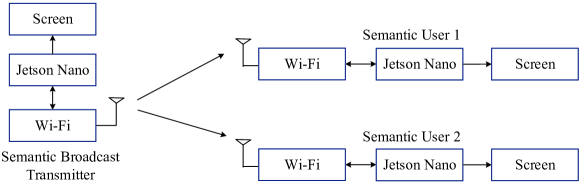
(a)

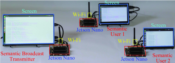
(b)

Figure 7: (a) The architecture of the semantic broadcast network prototype with two users; (b) The hardware platform of the semantic broadcast network prototype with two users.

The proposed semantic broadcast network prototype architecture and the hardware platform design are, respectively, shown in Fig. 7 (a) and (b), which can be used to implement the proposed features-disentangled semantic broadcast network in Fig. 6. The proposed semantic broadcast network prototype includes one transmitter and two semantic mobile users, i.e., User 1 and User 2. The trained semantic broadcast network is implemented using three portable Jetson Nano B01 processors, which represent the transmitter, User $1$ and User $2$. The detailed parameters of the portable Jetson Nano B01 prototype are provided in Table II, which is equipped with NVIDIA Maxwell graphics processing unit (GPU) architecture with 128 NVIDIA A cores, an ARM Cortex - A57 MPcore @quad-core CPU, Wi-Fi, Pytorch-GPU and torch-vision software.

Specifically, the transmitter performs semantic encoding on the input data, and then does feature selection and bit-level source and channel encoding, and finally broadcasts the semantic feature data to User $1$ and $2$ via Wi-Fi. With received data through Wi-Fi, User $1$ first performs bit-level channel and source decoding, and then does feature completion, followed by semantic decoding, and finally the decoded data is displayed. The operation of User $2$ is similar to that of User $1$.

TABLE II: Hardware parameters of the semantic BC network prototype.

GPU	NVIDIA Maxwell architecture
	128-NVIDIA-CUDA-core
CPU	Quad-core Cortex-A57
Memory	4GB LPDDR4
Wi-Fi	2.4GHz IEEE 802.11n$/$g$/$b
Screen	1920*1080px/800*480px display

VI Experiments Results and Analysis

In this section, the experimental performance of the proposed feature disentangled semantic broadcast network is evaluated via both the GPU simulation and the hardware prototype. The GPU experiments in this work have been performed on 502 GB RAM Intel Xeon Gold 6240 CPU, and 24 GB Nvidia GeForce 3090 GTX graphics card with Pytorch powered with CUDA 11.3. We adopt the Adam optimizer[39] with a batch size 16 and an initial learning rate of 0.0001. The experiments are performed through two standard datasets, i.e., Fonts Dataset[36] and ilab-20M Dataset[40].

VI-A Demonstration of Semantic BC Performance via GPU Simulation

The robust transmission performance of the proposed semantic BC scheme is demonstrated over additive non-Gaussian distributed noise channels and slow Rayleigh fading channels. Moreover, four BC transmission schemes are compared, i.e., the JPEG based BC scheme, which uses the JPEG compression in digital communications, non-robust semantic BC scheme, where no channel noise is added to the training process, the proposed robust semantic BC scheme with ${\rm{SNR}}_{{\rm{train}}}=4{\rm{dB}}$, and the proposed robust semantic BC scheme with ${\rm{SNR}}_{{\rm{train}}}=8{\rm{dB}}$, where ${\rm{SNR}}_{{\rm{train}}}$ represents the training SNR of the scheme.

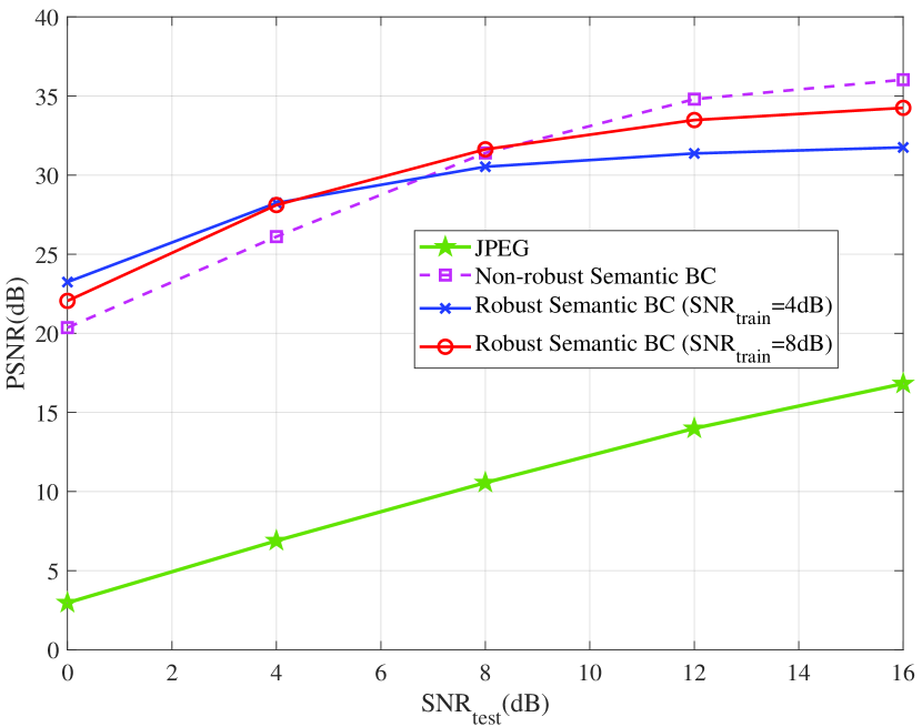
(a)

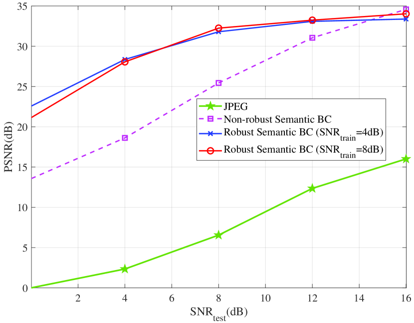
(b)

Figure 8: (a) PSNRs of the four schemes versus ${\rm{SNR}}_{{\rm{test}}}$ over ANGC; (b) PSNRs of the four schemes versus ${\rm{SNR}}_{{\rm{test}}}$ over over Rayleigh fading channels.

Fig. 8 (a) depicts peak signal-to-noise ratios (PSNRs) of the four BC schemes versus test SNRs ${\rm{SNR}}_{{\rm{test}}}$ over ANGC, where the PDFs of the additive non-Gaussian distributed noise ${N_{1,s}}$ and ${N_{2,s}}$ are ${p_{{N_{1,{\rm{s}}}}}}\left(x\right)={p_{{N_{2,{\rm{s}}}}}}\left(x\right)=\frac{5}{2}\left({{\rm{erf}}\left({\frac{{1-10x}}{{10\sqrt{2}}}}\right)-{\rm{erf}}\left({\frac{{-1-10x}}{{10\sqrt{2}}}}\right)}\right)$. As it can be observed, the PSNR of the JPEG compression scheme is significantly lower than those of the other three schemes. In the low SNR region (${\rm{SN}}{{\rm{R}}_{{\rm{test}}}}\leq 4{\rm{dB}}$), the PSNR of the robust semantic BC scheme with ${\rm{SNR}}_{{\rm{train}}}=4{\rm{dB}}$ is the highest, and PSNR of the robust semantic BC scheme with ${\rm{SNR}}_{{\rm{train}}}=8{\rm{dB}}$ is higher than that of the non-robust semantic BC scheme. For the medium SNR region ($4{\rm{dB}}\leq{\rm{SN}}{{\rm{R}}_{{\rm{test}}}}\leq 8{\rm{dB}}$), the PSNR of the robust semantic BC scheme with ${\rm{SNR}}_{{\rm{train}}}=8{\rm{dB}}$ is the highest, which verifies the robustness of the proposed schemes especially for low and medium SNR regions. For the high SNR region (${\rm{SN}}{{\rm{R}}_{{\rm{test}}}}\geq 8{\rm{dB}}$), the PSNR of the non-robust semantic BC scheme is the highest. This is because the influence of noise can be neglected in the high SNR region.

Fig. 8 (b) shows PSNRs of the four BC schemes versus test SNRs (${\rm{SNR}}_{{\rm{test}}}$) over slow Rayleigh fading channels, where ${G_{1}}\sim\mathcal{N}\left({0,1}\right)$ and ${G_{2}}\sim\mathcal{N}\left({0,2}\right)$. Similar to PSNR performance in Fig. 8 (a), JPEG compression has the worst performance among the four schemes. When ${\rm{SN}}{{\rm{R}}_{{\rm{test}}}}\leq 15{\rm{dB}}$, the PSNRs of the proposed robust semantic BC schemes with ${\rm{SNR}}_{{\rm{train}}}=4{\rm{dB}}$ and ${\rm{SNR}}_{{\rm{train}}}=8{\rm{dB}}$ are higher than that of the non-robust semantic BC scheme, which also demonstrates the robustness of the proposed schemes. While for ${\rm{SN}}{{\rm{R}}_{{\rm{test}}}}\geq 15{\rm{dB}}$, the PSNR of the non-robust semantic BC scheme is the highest, because the noise effect can be neglected.

TABLE III: Performance comparison of the semantic BC network over ANGC

Input data ${X_{\rm{d}}}$	Users	Intended feature	Knowledge base	JPEG	Non-robust semantic BC	Robust semantic BC ${\rm{SNR}}_{{\rm{train}}}=4{\rm{dB}}$	Robust semantic BC ${\rm{SNR}}_{{\rm{train}}}=8{\rm{dB}}$
	User 1 ${\rm{SNR}}_{{\rm{test}}}=4{\rm{dB}}$	Content
	User 2 ${\rm{SNR}}_{{\rm{test}}}=8{\rm{dB}}$	Font color
	User 1 ${\rm{SNR}}_{{\rm{test}}}=4{\rm{dB}}$	Content
	User 2 ${\rm{SNR}}_{{\rm{test}}}=8{\rm{dB}}$	Pose

TABLE IV: Performance comparison of the semantic BC network over Rayleigh fading channels

Input data ${X_{\rm{d}}}$	Users	Interest feature	Knowledge base	JPEG	Non-robust semantic BC	Robust semantic BC ${\rm{SNR}}_{{\rm{train}}}=4{\rm{dB}}$	Robust semantic BC ${\rm{SNR}}_{{\rm{train}}}=8{\rm{dB}}$
	User 1 ${\rm{SNR}}_{{\rm{test}}}=4{\rm{dB}}$	Content
	User 2 ${\rm{SNR}}_{{\rm{test}}}=8{\rm{dB}}$	Font color
	User 1 ${\rm{SNR}}_{{\rm{test}}}=4{\rm{dB}}$	Content
	User 2 ${\rm{SNR}}_{{\rm{test}}}=8{\rm{dB}}$	Pose

Table III shows performance comparison of the semantic BC network with two users, i.e., User 1 with ${\rm{SNR}}_{{\rm{test}}}=4{\rm{dB}}$ and User 2 with ${\rm{SNR}}_{{\rm{test}}}=8{\rm{dB}}$, over the ANGC, where the intended features and the knowledge bases of the two users are different. Specifically, as shown in the first two rows, the input data is a red lowercase letter $w$ on blue background image, and the third column shows that the intended features of Users $1$ and $2$ are content and font color, respectively. The fourth column shows that the knowledge bases of Users $1$ and $2$ are a green uppercase letter $U$ on yellow background, and a yellow uppercase letter $E$ on gray background, respectively. The fifth column shows the poor transmission performance of the JPEG compression scheme, where the decoded images cannot be recognized. The sixth to eighth columns are the reconstructed images of the non-robust semantic BC scheme, the robust semantic BC scheme with ${\rm{SNR}}_{{\rm{train}}}=4{\rm{dB}}$, and the robust semantic BC scheme with ${\rm{SNR}}_{{\rm{train}}}=8{\rm{dB}}$, respectively. The reconstructed data of User 1 is a green lowercase letter $w$ on yellow background, and the reconstructed data of User 2 is a red uppercase letter $E$ on gray background, which verifies the effectiveness of the feature selection and feature completion of the proposed semantic BC network.

Moreover, the input data of the last two rows in Table III is a white bus with lower-left-pose image, and the third column shows that the intended features of Users $1$ and $2$ are content and pose, respectively. The fourth column shows that the knowledge bases of Users $1$ and $2$ are a left-pose car with red-white-green color, and a red pickup truck with upper-right-pose, respectively. Similarly, the fifth column shows the decoded images of the JPEG compression scheme cannot be recognized. The sixth to eighth columns show that the reconstructed data of Users 1 and $2$ includes intended features and the features of the users’ knowledge bases, where only the intended features are transmitted. This also verifies the effectiveness of the feature selection and feature completion of the proposed semantic BC network.

Table IV shows performance comparison of the four BC schemes over the Rayleigh fading channels. Similar to Table III, Table IV demonstrates the effectiveness of the feature selection and feature completion of the proposed semantic BC network. Moreover, the sixth column shows that the reconstructed data of User 1 with the non-robust semantic BC scheme is blurry, while the reconstructed data of the robust semantic BC schemes are clear, which validates the added value of the robust semantic BC design.

VI-B Demonstration of Semantic BC Performance Via Prototype Experiment

TABLE V: Feature selection performance of the semantic BC network prototype

Input data ${X_{\rm{d}}}$	Users	Intended feature	Knowledge base	Reconstructed data ${\widehat{X}_{i,{\rm{d}}}}$ (Jetson Nano)
	User 1	Content
	User 2	Style
	User 1	Content
	User 2	Pose

The performance of the features-disentangled semantic BC networks are demonstrated via the proposed semantic BC prototype, which was designed in Section VI,

Table V shows feature selection performance of the semantic BC network, where the intended features and the knowledge bases of Users $1$ and $2$ are different. Specifically, the input data of the first two rows is a small size blue letter $F$ in italics, and the third column shows that the intended features of Users $1$ and $2$ are content and style, respectively. The fourth column shows that the knowledge bases of Users $1$ and $2$ are a large size pink letter $U$ in regular font, and a large size red letter $T$ in regular font, respectively. The fifth column shows that the reconstructed image of User 1 is a large size pink letter $F$ in regular font, and the reconstructed data of User 2 is a small size red letter $T$ in italics. Thus, only the intended semantic features are transmitted to users, and the unintended semantic features are generated based on the knowledge base. Moreover, the input data of the last two rows is a red left pose car. Similarly, column 3 to column 5 also verify the effectiveness of the feature selection and feature completion of the proposed semantic BC network.

TABLE VI: Transmission comparison over the semantic BC network prototype

	Transmission time (ms)	Compression ratio	PSNR	Reconstructed data
Original image	466.44	1	100
JPEG	168.69	21.22	23.72
Non-robust Semantic BC	5	1966.09	27.59
Robust Semantic BC ${\rm{SNR}}_{{\rm{test}}}=8{\rm{dB}}$	5	1966.09	27.32

Finally, in Table VI, we present the transmission time (ms), compression ratio, PSNR and reconstructed data of the original image transmission scheme, JPEG compression scheme, non-robust semantic BC scheme, and robust semantic BC scheme with ${\rm{SNR}}_{{\rm{train}}}=8{\rm{dB}}$. Table VI shows that the transmission time of the non-robust semantic BC scheme, and robust semantic BC scheme are $5$ ms significantly lower than those of the JPEG compression scheme (168.69 ms) and the original image transmission scheme (466.44 ms). Moreover, the compression ratio of the non-robust semantic BC scheme, and the robust semantic BC scheme are $1966.09$ significantly higher than those of the JPEG compression scheme (21.22) and the original image transmission scheme. Therefore, the proposed semantic BC network can significantly reduce the transmission load and transmission time. Moreover, the PSNRs of the robust semantic BC scheme is higher than that of the JPEG compression scheme, and is close to that of the non-robust BC scheme.

VII Conclusions

In this paper, we proposed a practical robust features-disentangled semantic BC framework, which can take advantage of the existing well-designed standards and hardware of bit-level communication networks. In our proposed framework, the semantic information was extracted and decoupled into independent semantic features. Then, by applying features selection, only semantic features of interest to users are selected for transmission, and the remaining semantic features need not be sent, which not only reduces the BC network load, but also enhances the robustness of the semantic features to channel noise. Moreover, we presented the optimal distortions allocation scheme for multi-source data compression, and derived both inner and outer bounds for the achievable rates region semantic broadcast channels. Furthermore, we designed a lightweight robust semantic BC network based on the supervised AE, and developed the corresponding hardware proof-of-concept prototype, which is the first prototype of the semantic BC network. Finally, both GPU simulation and prototype experiments demonstrated that our proposed semantic BC network is robust to both channel noise and channel fading, and can significantly improve transmission efficiency. This paper demonstrates the viability of a semantic BC network design and its practical implementation.

References

- [1] Y. S. J. Z. K. B. Letaief W. Chen. and Y. J. A. Zhang, “The roadmap to 6G: AI empowered wireless networks,” IEEE Commun. Mag., vol. 57, no. 8, pp. 84–90, Aug. 2019.
- [2] P. Zhang, W. Xu, H. Gao, K. Niu, X. Xu, X. Qin, C. Yuan, Z. Qin, H. Zhao, J. Wei, et al., “Toward wisdom-evolutionary and primitive-concise 6G: A new paradigm of semantic communication networks,” Engineering, 2022.
- [3] M. Kountouris and N. Pappas, “Semantics-empowered communication for networked intelligent systems,” IEEE Commun. Mag., vol. 59, no. 6, pp. 96–102, Jan. 2021.
- [4] W. B. M. Furuya R. Sterling. and Y. Inoue, “D-ila full resolution 8k projector,” in SMPTE Annual Tech Conference Expo, 2009.
- [5] Cisco, “Annual internet report (2018-2023) white paper,” 2020.
- [6] I. Union, “IMT traffic estimates for the years 2020 to 2030,” in Report ITU, 2015.
- [7] B. Mao, F. Tang, Y. Kawamoto, and N. Kato, “AI models for green communications towards 6G,” IEEE Commun. Surveys Tuts., vol. 24, no. 1, pp. 210–247, Nov. 2022.
- [8] K. Niu, J. Dai, S. Yao, S. Wang, Z. Si, X. Qin, and P. Zhang, “Towards semantic communications: A paradigm shift,” arXiv preprint arXiv:2203.06692, 2022.
- [9] M. Sana and E. Calvanese Strinati, “Learning semantics: An opportunity for effective 6G communications,” arXiv preprint arXiv:2202.11958, 2021.
- [10] Y. L. G. Shi Y. Xiao. and X. Xie, “From semantic communication to semantic-aware networking: Model, architecture, and open problems,” IEEE Commun. Mag., vol. 59, no. 8, pp. 44–50, Aug. 2021.
- [11] X. Luo, H.-H. Chen, and Q. Guo, “Semantic communications: Overview, open issues, and future research directions,” IEEE Wirel. Commun., pp. 1–10, Jan. 2022.
- [12] J. Bao, P. Basu, M. Dean, C. Partridge, A. Swami, W. Leland, and J. A. Hendler, “Towards a theory of semantic communication,” in Proc. IEEE Netw. Sci. Workshop, pp. 110–117, Jun. 2011.
- [13] A. Y. B. Güler and A. Swami, “The semantic communication game,” IEEE Trans. Cogn. Commun. Netw., vol. 4, no. 4, pp. 787–802, Dec. 2018.
- [14] N. Farsad, M. Rao, and A. Goldsmith, “Deep learning for joint source-channel coding of text,” in Proc.(ICASSP), pp. 2326–2330, Apr. 2018.
- [15] H. Xie, Z. Qin, L. Geoffrey Ye., and B.-H. Juang, “Deep learning enabled semantic communication systems,” IEEE Trans. Signal Process., vol. 69, pp. 2663–2675, Apr. 2021.
- [16] P. Jiang, C.-K. Wen, S. Jin, and G. Y. Li, “Deep source-channel coding for sentence semantic transmission with HARQ,” arXiv preprint arXiv:2106.03009, 2021.
- [17] K. Lu, R. Li, X. Chen, Z. Zhao, and H. Zhang, “Reinforcement learning-powered semantic communication via semantic similarity,” arXiv preprint arXiv:2108.12121, 2021.
- [18] Z. Weng and Z. Qin, “Semantic communication systems for speech transmission,” IEEE J. Sel. Areas Commun., vol. 39, no. 8, pp. 2434–2444, Aug. 2021.
- [19] H. Tong, Z. Yang, S. Wang, Y. Hu, W. Saad, and C. Yin, “Federated learning based audio semantic communication over wireless networks,” in Proc. IEEE Global Commun. Conf. (GLOBECOM), pp. 1–6, Feb. 2021.
- [20] G. Shi, D. Gao, X. Song, J. Chai, M. Yang, X. Xie, L. Li, and X. Li, “A new communication paradigm: from bit accuracy to semantic fidelity,” arXiv preprint arXiv:2101.12649, Jan. 2021.
- [21] P. Jiang, C.-K. Wen, S. Jin, and G. Y. Li, “Wireless semantic communications for video conferencing,” arXiv preprint arXiv:2204.07790, 2022.
- [22] T.-Y. Tung and D. Gündüz, “Deepwive: Deep-learning-aided wireless video transmission,” arXiv preprint arXiv:2111.13034, Nov. 2021.
- [23] D. B. Kurka and D. Gündüz, “Bandwidth-agile image transmission with deep joint source-channel coding,” IEEE Trans. Wireless Commun., vol. 20, no. 12, pp. 8081–8095, Jun. 2021.
- [24] M. Jankowski, D. Gündüz, and K. Mikolajczyk, “Wireless image retrieval at the edge,” IEEE J. Sel. Areas Commun., vol. 39, no. 1, pp. 89–100, Jan. 2021.
- [25] Y. M. J. Shao and J. Zhang, “Learning task-oriented communication for edge inference: An information bottleneck approach,” IEEE J. Sel. Areas Commun., vol. 40, no. 1, pp. 197–211, Jan. 2022.
- [26] X. Kang, B. Song, J. Guo, Z. Qin, and F. R. Yu, “Task-oriented image transmission for scene classification in unmanned aerial systems,” arXiv preprint arXiv:2112.10948, Dec. 2021.
- [27] Q. Hu, G. Zhang, Z. Qin, Y. Cai, and G. Yu, “Robust semantic communications against semantic noise,” arXiv preprint arXiv:2202.03338, Feb. 2022.
- [28] D. Huang, X. Tao, F. Gao, and J. Lu, “Deep learning-based image semantic coding for semantic communications,” in 2021 IEEE Global Communications Conference (GLOBECOM), pp. 1–6, Dec. 2021.
- [29] E. Bourtsoulatze, D. B. Kurka, and D. Gündüz, “Deep joint source-channel coding for wireless image transmission,” IEEE Trans. Cognit.Commun. Netw., vol. 5, no. 3, pp. 567–579, May. 2019.
- [30] J. Xu, B. Ai, W. Chen, A. Yang, P. Sun, and M. Rodrigues, “Wireless image transmission using deep source channel coding with attention modules,” IEEE Trans. Circuits Syst. Video Technol., May. 2021.
- [31] D. B. Kurka and D. Gündüz, “Deepjscc-f: Deep joint source-channel coding of images with feedback,” IEEE J. Sel. Areas Inf. Theory, vol. 1, no. 1, pp. 178–193, Apr. 2020.
- [32] M. Yang, C. Bian, and H.-S. Kim, “OFDM-guided deep joint source channel coding for wireless multipath fading channels,” IEEE Trans. Cognit. Commun. Netw., Feb. 2022.
- [33] M. Yang and H.-S. Kim, “Deep joint source-channel coding for wireless image transmission with adaptive rate control,” arXiv preprint arXiv:2110.04456, 2021.
- [34] M. Ding, J. Li, M. Ma, and X. Fan, “SNR-adaptive deep joint source-channel coding for wireless image transmission,” in Proc. IEEE Int. Conf. Acoust., Speech, Signal Process.(ICASSP), pp. 1555–1559, May. 2021.
- [35] Y. Blau and T. Michaeli, “Rethinking lossy compression: The rate-distortion-perception tradeoff,” in International Conference on Machine Learning. PMLR, pp. 675–685, 2019.
- [36] G. X. L. I. Yunhao Ge Sami Abu-El-Haija., “Zero-shot synthesis with group-supervised learning,” Proc. ICLR, pp. 1–16, 2021.
- [37] T. M. Cover and J. A. Thomas, Elements of information theory, 2nd ed., New York, NY, USA: Wiley, 2006.
- [38] S. Ihara, “On the capacity of channels with additive non-Gaussian noise,” Inform. Contr., vol. 37, no. 1, pp. 34–39, Sep. 1978.
- [39] J. B. Diederik P. Kingma, “Adam: a method for stochastic optimization,” arXiv preprint arXiv:1412.6980, 2014.
- [40] A. Borji, S. Izadi, and L. Itti, “ilab-20m: A large-scale controlled object dataset to investigate deep learning,” in 2016 IEEE Conference on Computer Vision and Pattern Recognition (CVPR), pp. 2221–2230, 2016.