Scale invariant bounds for mixing in the Rayleigh-Taylor instability

Abstract

We study the Rayleigh-Taylor instability for two miscible, incompressible, inviscid fluids. Scale-invariant estimates for the size of the mixing zone and coarsening of internal structures in the fully nonlinear regime are established following techniques introduced for the Saffman-Taylor instability in [11]. These bounds provide optimal scaling laws and reveal the strong role of dissipation in slowing down mixing.

Keywords.

Rayleigh-Taylor instability, Saffman-Taylor instability, fluid mixing.

1 Introduction

We consider an infinite column of two fluids of densities $\rho_{+}>\rho_{-}>0$ in a gravitational field, initially arranged so that the heavy fluid is on top. The interface between the fluids is unstable and any small perturbation leads to turbulent mixing. This stability problem was first studied by Rayleigh [10] and then analyzed again in Taylor’s work [15] (see also [6]). The Rayleigh-Taylor instability occurs in several natural settings (e.g. collapse of massive stars, formation of clouds) and technological applications (e.g. laser and electromagnetic implosions) (see [14, 16, 17] for reviews).

The following three stages of evolution are observed in experiments and numerical simulations. In an early stage, the growth of the instability is determined by linear analysis [15]. This is followed by a fully nonlinear scaling regime where the turbulent mixing zone grows at the rate $\alpha_{\pm}At^{2}$, where $A=(\rho_{+}-\rho_{-})/(\rho_{+}+\rho_{-})$ is the Atwood number and $\alpha_{\pm}$ are empirically determined constants corresponding to the upper and lower edges of the mixing zone. This stage is also characterized by the formation of internal structures that have been termed bubbles and spikes. Finally, there is a late stage dominated by dissipation. In miscible and inviscid fluids, this dissipation is caused by molecular diffusion.

This paper provides rigorous results in the fully nonlinear regime and the late stage of the Rayleigh-Taylor instability that is based on the underlying partial differential equations. We use bulk quantities, energy balance and an interpolation inequality to estimate the size of the mixing zone. Our results also predict the coarsening rate of bubbles and spikes. Finally, a modification of these arguments is used to understand the crossover from the regime of turbulent mixing to the dissipative regime, when molecular diffusion acts to slow down mixing. Our results are consistent with a recent rigorous analysis by Gebhard et al  [7]. However, our work follows methods introduced in [11], whereas the results in [7] rely on convex integration. While there is an extensive literature on the early stage of the instability, to the best of our knowledge, article [7] and this paper are the first rigorous results on the fully nonlinear regime that accord with experiments.

1.1 The main model

We model the evolution of the Rayleigh-Taylor instability for miscible, inviscid, incompressible fluids with the following system of PDEs

$$\rho_{t}+{\mathbf{u}}\cdot\nabla\rho-\Delta\rho=0,$$ (1)

$$\rho({\mathbf{u}}_{t}+({\mathbf{u}}\cdot\nabla){\mathbf{u}})-(\nabla\rho\cdot\nabla){\mathbf{u}}+\nabla p+\rho g\mathbf{e}_{z}=0, \nabla\cdot{\mathbf{u}}=0.$$ (2)

Here $\rho$ is the density, ${\mathbf{u}}$ is the velocity field, $g$ is the acceleration which is normalized to unity, $p$ is the pressure, and $\mathbf{e}_{z}$ is the unit vector in the vertical direction. Equations (1)-(2) are posed in an infinite strip $[0,L]^{d-1}\times\mathbb{R}\ni x=(y,z)$. $L$ plays a role of the Peclet number and quantifies the effect of miscibility. We assume periodic boundary conditions in the transverse direction $y$.

The model consists of an advection-diffusion equation (1) for the density $\rho$ coupled with the incompressible Euler equations (2) for the velocity ${\mathbf{u}}$ and pressure $p$. The diffusion term in equation (1) models miscibility. The inclusion of diffusion in equation (1) also requires the inclusion of an additional term in the momentum equation (2), corresponding to the transport driven by diffusion. This ensures energy balance as a fundamental law, as shown in Lemma 1. Diffusion regularizes the evolution and causes the coarsening of bubbles and spikes as quantified in Theorem 2.

We do not consider the effect of viscosity in this paper. In fact, the interplay between molecular diffusion and viscosity in the Rayleigh-Taylor instability is quite subtle, and several competing models have been proposed such as the variable density model (VDM). The VDM is based on Fickian diffusion which leads to artificial compressibility and, hence, to additional dissipation mechanisms (see [2] for a review and [8] for an analysis).

The steady, perfectly stratified state is

$${\mathbf{u}}_{0}=0,\;\rho_{0}=\begin{cases}\rho_{+},&z\geqslant 0,\\ \rho_{-},&z<0.\end{cases}$$ (3)

This state serves as a reference configuration. Throughout this paper, the initial condition is a small perturbation of this state.

Let us outline our results informally. We obtain $L$-independent estimates on the potential energy, kinetic energy, mixing entropies, and mean perimeter for classical solutions to (1)-(2). These energy estimates may be interpreted as one-sided bounds

$$\alpha_{-}At^{2}\leq a_{-}(t),\quad a_{+}(t)\leq\alpha_{+}At^{2},\quad b_{\pm}(t)\geq\beta_{\pm}\sqrt{t},$$ (4)

where $a_{\pm}(t)$ measures the upper and lower edge of the mixing zone, $b_{\pm}(t)$ measures coarsening of structures within the mixing zone, and $\alpha_{\pm}$ and $\beta_{\pm}$ are universal constants depending on $A$ alone. See Figure 1 for a caricature of $a_{\pm}$ and $b_{\pm}$.

Figure 1: Caricature of the main scales

Explicit formulas for the constants $\alpha_{\pm}$ are derived and compared with experimental and numerical results in the area (see Remark 1). While our scaling laws are comparable with the experiments, the constants $\alpha_{\pm}$ are an order of magnitude below the experimental results. This gap may be due to the turbulent dissipation; the corresponding phenomenon for the Saffman-Taylor instability was termed dissipative slowdown, and sharp results were obtained for a reduced model in [11, 12]. It remains a challenge to obtain sharp bounds on the size of the mixing zone in both the Saffman-Taylor and Rayleigh-Taylor instability.

2 The main results

We state our results in this section.

2.1 Bulk quantities and notations

Let us first introduce notation for averaging and normalization. Given a scalar function $f:[0,L]^{d-1}\times\mathbb{R}\to\mathbb{R}$, we average it over the transverse direction

$$\bar{f}(z)=\frac{1}{L^{d-1}}\int_{[0,L]^{d-1}}f(y,z)\;dy.$$ (5)

In order to ensure $L$-independent estimates, we define normalized integrals

$$\mathchoice{{\vbox{\hbox{$\textstyle-$}}\kern-4.86108pt}}{{\vbox{\hbox{$\scriptstyle-$}}\kern-3.25pt}}{{\vbox{\hbox{$\scriptscriptstyle-$}}\kern-2.29166pt}}{{\vbox{\hbox{$\scriptscriptstyle-$}}\kern-1.875pt}}\!\int f(x)\;dx=\int_{\mathbb{R}}\frac{1}{L^{d-1}}\int_{[0,L]^{d-1}}f(y,z)\;dy\,dz.$$ (6)

The following non-dimensional $L$-independent bulk quantities play the key role in our analysis: the negative of the potential energy

$$E_{p}(t)=\frac{1}{\rho_{+}-\rho_{-}}\mathchoice{{\vbox{\hbox{$\textstyle-$}}\kern-4.86108pt}}{{\vbox{\hbox{$\scriptstyle-$}}\kern-3.25pt}}{{\vbox{\hbox{$\scriptscriptstyle-$}}\kern-2.29166pt}}{{\vbox{\hbox{$\scriptscriptstyle-$}}\kern-1.875pt}}\!\int(\rho_{0}(z)-\rho(x,t))z\;dx$$ (7)

and the kinetic energy of the fluid

$$E_{k}(t)=\frac{1}{2}\frac{1}{\rho_{+}-\rho_{-}}\mathchoice{{\vbox{\hbox{$\textstyle-$}}\kern-4.86108pt}}{{\vbox{\hbox{$\scriptstyle-$}}\kern-3.25pt}}{{\vbox{\hbox{$\scriptscriptstyle-$}}\kern-2.29166pt}}{{\vbox{\hbox{$\scriptscriptstyle-$}}\kern-1.875pt}}\!\int\rho(x,t)|{\mathbf{u}}(x,t)|^{2}\;dx.$$ (8)

We also consider the mixing entropies

$$H(t)=\frac{1}{(\rho_{+}-\rho_{-})^{2}}\mathchoice{{\vbox{\hbox{$\textstyle-$}}\kern-4.86108pt}}{{\vbox{\hbox{$\scriptstyle-$}}\kern-3.25pt}}{{\vbox{\hbox{$\scriptscriptstyle-$}}\kern-2.29166pt}}{{\vbox{\hbox{$\scriptscriptstyle-$}}\kern-1.875pt}}\!\int(\rho_{+}-\rho(x,t))(\rho(x,t)-\rho_{-})\;dx$$ (9)

and

$$S(t)= -\mathchoice{{\vbox{\hbox{$\textstyle-$}}\kern-4.86108pt}}{{\vbox{\hbox{$\scriptstyle-$}}\kern-3.25pt}}{{\vbox{\hbox{$\scriptscriptstyle-$}}\kern-2.29166pt}}{{\vbox{\hbox{$\scriptscriptstyle-$}}\kern-1.875pt}}\!\int\left[\frac{\rho_{+}-\rho(x,t)}{\rho_{+}-\rho_{-}}\log\left(\frac{\rho_{+}-\rho(x,t)}{\rho_{+}-\rho_{-}}\right)+\right.$$ (10)

$$\left.+\frac{\rho(x,t)-\rho_{-}}{\rho_{+}-\rho_{-}}\log\left(\frac{\rho(x,t)-\rho_{-}}{\rho_{+}-\rho_{-}}\right)\right]\;dx,$$

which measure size of ”mushy zones” where $\rho_{-}<\rho<\rho_{+}$. Note that $H(t)$ and $S(t)$ vanishes if $\rho\in\{\rho_{-},\rho_{+}\}$ a.e. By the maximum principle, incorporation of the diffusion term in (1) ensures $\rho\in(\rho_{-},\rho_{+})$ for all $x\in[0,L]^{d-1}\times\mathbb{R}$ and $t>0$. Thus, $H(t)$ is positive for all $t>0$.

Finally, we define the averaged perimeter to measure coarsening

$$P(t)=\frac{1}{\rho_{+}-\rho_{-}}\mathchoice{{\vbox{\hbox{$\textstyle-$}}\kern-4.86108pt}}{{\vbox{\hbox{$\scriptstyle-$}}\kern-3.25pt}}{{\vbox{\hbox{$\scriptscriptstyle-$}}\kern-2.29166pt}}{{\vbox{\hbox{$\scriptscriptstyle-$}}\kern-1.875pt}}\!\int|\nabla\rho(x,t)|\;dx=\frac{1}{\rho_{+}-\rho_{-}}\int_{0}^{1}\mathcal{H}^{n-1}[\rho^{-1}(\eta)]\;d\eta.$$ (11)

Here $\mathcal{H}^{n-1}$ is the $n-1$ Hausdorff measure and the second equality follows from the co-area formula. We add a multiplier $(\rho_{+}-\rho_{-})^{-\alpha}$, $\alpha\in\{1,2\}$ in the definition of the quantities (7)-(11) to make all the estimates non-dimensional.

Throughout the paper, we denote by $\dot{F}(t)$ the time derivative of a bulk quantity $F(t)$ and by $f_{t}(x,t)$, $f_{x}(x,t)$ the partial derivatives of a function $f(x,t)$.

2.2 Uniform bounds on bulk quantities

Theorem 1.

Let $(\rho,{\mathbf{u}})$ be a classical solution to (1)-(2) with initial data such that the initial potential energy $E_{p}(0)$, the mixing entropy $H(0)$, and the mean perimeter $P(0)$ are finite. Then

$$\limsup_{t\to+\infty}\frac{E_{p}(t)}{(At^{2})^{2}}\leqslant\frac{1}{24(1-A^{2})},$$ (12)

$$\limsup_{t\to+\infty}\frac{H(t)}{At^{2}}\leqslant\frac{1}{12\sqrt{1-A^{2}}},$$ (13)

and

$$\limsup_{t\to+\infty}\frac{1}{(At^{2})^{2}}\int_{0}^{t}P^{2}(\tau)\;d\tau\leqslant\frac{\pi}{36(1-A^{2})}.$$ (14)

Remark 1.

Theorem 1 provides a comparison between the bounds of the mixing zone and the Riemann problem, which is described below. Taking the entropy solution yields

$$\alpha_{+}=\frac{1}{1-A}\quad\mathrm{and}\quad\alpha_{-}=-\frac{1}{1+A}.$$ (15)

On the other hand, the weak solution consisting of two shocks suggests (formally)

$$\tilde{\alpha}_{+}=\frac{1}{1-A+\sqrt{1-A^{2}}},\quad\mathrm{and}\quad\tilde{\alpha}_{-}=-\frac{1}{1+A+\sqrt{1-A^{2}}}.$$ (16)

Existence of weak solutions that mix at this rate is established by Gebhard et al provided $A$ is sufficiently close to $1$. The construction in [7] also uses a scalar conservation law, but not the one with flux $g(s)$ defined in (25) below (see Section  3).

Remark 2.

Relation (14) is the integrated analog of the (unproven) asymptotic, pointwise inequality

$$P(t)\leqslant\frac{2\sqrt{\pi}}{3}\frac{A}{\sqrt{(1+A)(1-A)}}t^{3/2}.$$ (17)

It may be interpreted as a coarsening estimate by defining the following non-dimensional transverse length-scales

$$b_{+}(t)=\frac{a_{+}(t)}{P(t)},\quad b_{-}(t)=-\frac{a_{-}(t)}{P(t)}.$$ (18)

We use estimate (29), to obtain the lower bound

$$b_{+}(t)\geqslant\frac{3}{2\sqrt{\pi}}(1+A)t^{1/2},\quad b_{-}(t)\geqslant\frac{3}{2\sqrt{\pi}}(1-A)t^{1/2}.$$ (19)

Physically, this estimate means that we expect the average width of spikes and bubbles growth in time as $\sqrt{t}$. In the Saffman-Taylor instability, these coarsening rates are due to the merging of fingers. By analogy, we expect that in the Rayleigh-Taylor instability, these rates are determined by mergers of bubbles and spikes. The experimental reviews focus on $\alpha_{\pm}$ and the spreading of the mixing zone; coarsening rates appear not to have been measured systematically (see [1] for a broad range of experimental diagnostics).

2.3 A crossover effect

Theorem 1 gives an $L$-independent estimate on the potential energy. A strict use of $L$-independent estimates is necessary to obtain self-similar mixing. Our techniques also admit a natural $L$-dependent modification which describes the late stage of the Rayleigh-Taylor instability.

Theorem 2.

Let $(\rho,{\mathbf{u}})$ be a classical solution to (1)-(2) with initial data such that the initial potential energy $E_{p}(0)$, the mixing entropy $H(0)$, and the mean perimeter $P(0)$ are finite. Then

$$\limsup\limits_{t\to+\infty}\frac{E_{p}(t)}{(At^{3/2})^{2}}\lesssim\frac{L^{2}}{(1-A)^{3/2}}.$$ (20)

Estimate from the Theorem 2 is sharper than the $L$-independent version from Theorem 1 when

$$t\gtrsim\frac{L^{2}}{(1-A)^{1/2}}.$$ (21)

This is the time scale when dissipation dominates convective transport.

3 The Riemann problem and some comparisons

3.1 Connection with scalar conservation laws

Theorem 1 allows to compare the classical solution to (1)-(2) with a solution to a Riemann problem. This idea was introduced in [13] and underlies [11, 12]. In order to simplify the analysis, we define a function $\chi:[0,L]^{d-1}\times\mathbb{R}\to[0,1]$ such that

$$\rho=\rho_{-}\chi+\rho_{+}(1-\chi),$$ (22)

and $s:\mathbb{R}\to[0,1]$ by $s=\bar{\chi}$. Then

$$\bar{\rho}=\rho_{-}s+\rho_{+}(1-s).$$ (23)

The ideal mixing zone corresponds to solutions to the scalar conservation law

$$s_{\tau}+(g(s))_{z}=0,\quad\tau=t^{2}/2,$$ (24)

with the concave flux function $g:[0,1]\to[0,+\infty)$

$$g(s)=(\rho_{+}-\rho_{-})\frac{s(1-s)}{\rho_{+}s+\rho_{-}(1-s)}$$ (25)

and the Riemann initial data

$$s_{0}=\begin{cases}1,&z\leqslant 0,\\ 0,&z>0.\end{cases}$$ (26)

This Riemann problem has no classical solutions, but it has infinitely many weak solutions. Bounds (15) correspond to the rarefaction wave solution, whereas bounds (16) correspond to the two-shock solution. In the theory of scalar conservation laws, it is conventional to single out the rarefaction wave as the unique entropy solution to the Riemann problem [3]. However, in our work the Riemann problem arises through an averaging procedure, and these criterion cannot be naively applied.

We now compute these solutions. The rarefaction wave is self-similar and is given in terms of the similarity variable $\xi=z/\tau$ by

$$s(\xi)=\begin{cases}1,&\xi\leqslant-\frac{2A}{1+A},\\ (g^{\prime})^{-1}(\xi),&-\frac{2A}{1+A}<\xi\leqslant\frac{2A}{1-A},\\ 0,&\xi>\frac{2A}{1-A},\end{cases}$$ (27)

where the rarefaction profile is given by

$$(g^{\prime})^{-1}(\xi)=\frac{1-A}{2A}\left(\sqrt{\frac{1+A}{1-A}}\frac{1}{\sqrt{1+\xi}}-1\right),\;\xi\in\left[-\frac{2A}{1+A},\frac{2A}{1-A}\right].$$ (28)

This profile gives the following bound of the mixing zone

$$a_{+}(t)=\frac{A}{2}\frac{\rho_{+}+\rho_{-}}{\rho_{-}}t^{2}=\frac{At^{2}}{1-A}, a_{-}(t)=-\frac{A}{2}\frac{\rho_{+}+\rho_{-}}{\rho_{+}}t^{2}=-\frac{At^{2}}{1+A}.$$ (29)

The flux function $g(s)$ is concave and has its maximum at $s_{*}=\sqrt{\rho_{-}}/(\sqrt{\rho_{+}}+\sqrt{\rho_{-}})$. Motivated by the proof of Theorem 3 (see Lemma 7 for the details), we also define a two-shock solution connecting the states $1$, $s_{*}$ and $0$ by

$$s(\xi)=\begin{cases}1,&\xi\leqslant-\frac{2A}{1+A+\sqrt{1-A^{2}}},\\ \frac{\sqrt{1-A}}{\sqrt{1+A}+\sqrt{1-A}},&-\frac{2A}{1+A+\sqrt{1-A^{2}}}<\xi\leqslant\frac{2A}{1-A+\sqrt{1-A^{2}}},\\ 0,&\frac{2A}{1-A+\sqrt{1-A^{2}}}<\xi.\end{cases}$$ (30)

This solution provides the following bounds

$$\tilde{a}_{+}=\frac{A}{2}\frac{\rho_{+}+\rho_{-}}{\sqrt{\rho_{-}}(\sqrt{\rho_{+}}+\sqrt{\rho_{-}})}t^{2}=\frac{At^{2}}{1-A+\sqrt{1-A^{2}}},$$ (31)

$$\tilde{a}_{-}=-\frac{A}{2}\frac{\rho_{+}+\rho_{-}}{\sqrt{\rho_{+}}(\sqrt{\rho_{+}}+\sqrt{\rho_{-}})}t^{2}=-\frac{At^{2}}{1+A+\sqrt{1-A^{2}}}.$$ (32)

The rarefaction and shock profiles are compared in Figure 2. It is immediate that the two-shock solutions gives a smaller mixing zone. These two solutions correspond to two different hypotheses on the structure of a homogenized mixing zone. When considering the two-shock solution, we assume that there is a perfectly mixed zone without any $z$ variation. When considering the rarefaction wave we obtain a mixing zone that varies gradually with $z$.

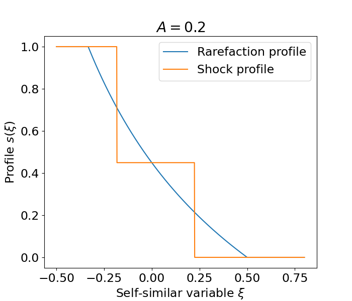
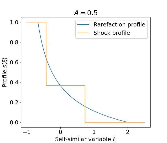
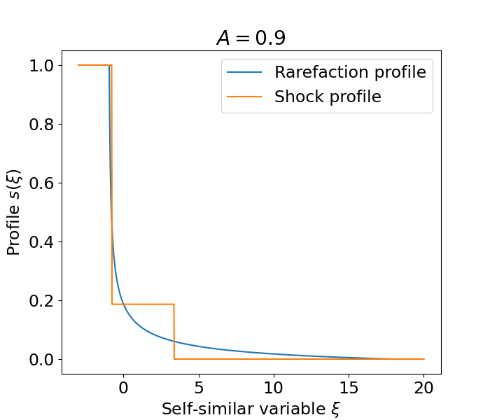
Figure 2: Comparison of the rarefaction (blue) and two-shock (red) profiles in the similarity variable $\xi=x/\tau=2x/t^{2}$ for different values of $A$.

Which, if either, of these two solutions correspond to experimental observations? In the case of the Saffman-Taylor instability, a reduced model was introduced and a maximum principle was established that shows (in effect) that it is the two shock structure that reflects the structure of the mixing zone. This phenomena was termed diffusive slowdown. The Rayleigh-Taylor instability is considerably more complicated. Let us now contrast the results obtained in [7] with Theorem 1.

3.2 Comparison with weak solutions constructed by convex integration

The $L$-independent upper bounds apply to any classical solution satisfying the hypothesis of Theorem 1. In particular, any weak solution to the immiscible problem obtained as a limit of a sequence of $L$-dependent classical solutions as $L\to\infty$ must also satisfy these bounds. In contrast, Gebhard et al [7] use convex integration to construct weak subsolutions to the immiscible equation

$$\rho_{t}+\nabla\cdot(\rho{\mathbf{u}})=0,$$ (33)

$$(\rho{\mathbf{u}})_{t}+\nabla\cdot(\rho{\mathbf{u}}\otimes{\mathbf{u}})+\nabla p+\rho g\mathbf{e}_{z}=0, \nabla\cdot{\mathbf{u}}=0,$$ (34)

for the finite time interval $(0,T)$ with $T>0$ in the finite strip $\Omega=(0,1)\times(-c_{-}(T),c_{+}(T))$. Function $c_{\pm}(t)$ are given by

$$c_{\pm}(t)=\frac{\rho_{+}+\rho_{-}}{2\sqrt{\rho_{\mp}}(\sqrt{\rho_{+}}+\sqrt{\rho_{-}})}Agt^{2},$$ (35)

and the initial condition is given by perturbation of the flat interface (3) such that $\rho(x,0)\in\{\rho_{-},\rho_{+}\}$ a.e. The main result (see [7, Theorems 2.4 and 2.7]) provides existence of infinitely many bounded admissible weak solutions satisfying $\rho\in\{\rho_{-},\rho_{+}\}$ a.e which are mixing within the region $-c_{-}(t)<z<c_{+}(t)$, $t\in(0,T)$.

For such weak solutions to the immiscible system (33)-(34), the transverse averaged profile was obtained. If $\bar{\rho}(z,t)$ is the transverse average and $\tau=t^{2}/2$, $\bar{\rho}$ satisfies

$$\bar{\rho}_{\tau}+(G_{0}(\bar{\rho}))_{z}=0,$$ (36)

with the Riemann initial data. The limiting flux function corresponding to the boundary of the convex hull is given by (see [7, page 1274] for the details)

$$G_{0}(\rho)=-\frac{(\rho_{+}-\rho)(\rho-\rho_{-})}{\rho_{+}+\rho_{-}+\sqrt{\rho_{+}\rho_{-}}-\rho},$$ (37)

and can be easily rewritten in terms of $s$,

$$G_{0}(s)=(\rho_{+}-\rho_{-})\frac{s(1-s)}{\rho_{+}s+\rho_{-}(1-s)+\sqrt{\rho_{+}\rho_{-}}}.$$ (38)

Taking the entropy solution to the Riemann problem with the flux function $G_{0}$ provides the bounds given by $c_{\pm}(t)$ ($\tilde{a}_{\pm}$ in out notation). It also gives the following expression for the (non-dimensionalized) negative part of the potential energy [7, pp. 1277]

$$\begin{split}\frac{E_{p}}{A^{2}t^{4}}&=\frac{1}{24}\frac{(\rho_{+}+\rho_{-})^{2}}{(\sqrt{\rho_{+}}+\sqrt{\rho_{-}})^{2}\sqrt{\rho_{+}\rho_{-}}}\\ &=\frac{1}{24}\frac{2}{\sqrt{1-A^{2}}(1+\sqrt{1-A^{2}})}\leqslant\frac{1}{24}\frac{1}{1-A^{2}},\end{split}$$ (39)

since $A\in(0,1)$. The last inequality provides comparison of bounds from Theorem 1 with the main result from [7].

3.3 Comparison with the experimental data

We present a comparison of the experimental $\alpha_{\pm}$ with coefficients obtained from (29) and (31)-(32) in Table 1 and Table 2. The experimental and numerical data follows the comprehensive recent review [1, Fig. 12]. We have also compared results from earlier reviews [4, 5] with our work.

A	$\alpha_{+}$ from (15)	$\alpha_{+}$ from (16)	Observed $\alpha_{+}$
$0.0025$	$1.0$	$0.5$	$0.065\pm 0.005$
$0.08$	$1.09$	$0.52$	$0.065\pm 0.005$
$0.15$	$1.18$	$0.54$	$0.06$
$0.2$	$1.25$	$0.56$	$0.055$
$0.25$	$1.33$	$0.58$	$0.06$
$0.4$	$1.67$	$0.66$	$0.06$
$0.46$	$1.79$	$0.69$	$0.06\pm 0.005$
$0.6$	$2.5$	$0.83$	$0.06\pm 0.005$
$0.72$	$3.57$	$1.03$	$0.04\pm 0.005$
$0.8$	$5.0$	$1.25$	$0.05$
$0.88$	$8.33$	$1.68$	$0.05$
$0.97$	$33.33$	$3.66$	$0.05$

Table 1: Variation of $\alpha_{+}$ with the Atwood number, $A$.

A	$-\alpha_{-}$ from (15)	$-\alpha_{-}$ from (16)	Observed $-\alpha_{-}$
$0.0025$	$1.0$	$0.5$	$0.065\pm 0.005$
$0.08$	$0.93$	$0.48$	$0.09\pm 0.005$
$0.15$	$0.87$	$0.47$	$0.067\pm 0.005$
$0.2$	$0.83$	$0.46$	$0.05\pm 0.005$
$0.25$	$0.8$	$0.45$	$0.07\pm 0.005$
$0.4$	$0.71$	$0.43$	$0.065$
$0.46$	$0.69$	$0.43$	$0.08\pm 0.01$
$0.6$	$0.62$	$0.42$	$0.09\pm 0.01$
$0.72$	$0.58$	$0.41$	$0.075\pm 0.015$
$0.8$	$0.56$	$0.42$	$0.11$
$0.88$	$0.53$	$0.42$	$0.12$
$0.97$	$0.51$	$0.45$	$0.14$

Table 2: Variation of $-\alpha_{-}$ with the Atwood number, $A$.

The experimental values of $\alpha_{\pm}$ are significantly less than the predictions. This gap reflects the complexity of the Rayleigh-Taylor instability and may arise from turbulent dissipation, as well as physical effects, including viscosity, that are not modeled by equations (1)–(2).

The parameter $\alpha_{+}$ is consistently smaller than the parameter $-\alpha_{-}$. This implies that bubbles tend to ascend more rapidly when the prefactor is smaller. Conversely, our estimations suggest $\alpha_{+}>-\alpha_{-}$. This disparity in asymmetry might arise from the influence of various dissipation mechanisms not accounted for in the current system (1)-(2). Finally, note that $-\alpha_{-}(A)$ converges to $t^{2}/2$ as $A$ approaches $1$. This limiting scenario corresponds to the free fall of liquid within the gravitational field.

4 Differential inequalities on energy and entropies

The first important tool in this paper are differential inequalities for energy and entropies. We start with

Lemma 1 (Energy balance).

Let $(\rho,{\mathbf{u}})$ be a classical solution to (1)-(2) with the potential energy $E_{p}(t)$ and the kinetic energy $E_{k}(t)$ defined in (7) and (8). Then we have

$$\dot{E}_{p}=1-\frac{1}{\rho_{+}-\rho_{-}}\mathchoice{{\vbox{\hbox{$\textstyle-$}}\kern-4.86108pt}}{{\vbox{\hbox{$\scriptstyle-$}}\kern-3.25pt}}{{\vbox{\hbox{$\scriptscriptstyle-$}}\kern-2.29166pt}}{{\vbox{\hbox{$\scriptscriptstyle-$}}\kern-1.875pt}}\!\int\rho({\mathbf{u}}\cdot\mathbf{e}_{z})\;dx,$$ (40)

$$\dot{E}_{k}=-\frac{1}{\rho_{+}-\rho_{-}}\mathchoice{{\vbox{\hbox{$\textstyle-$}}\kern-4.86108pt}}{{\vbox{\hbox{$\scriptstyle-$}}\kern-3.25pt}}{{\vbox{\hbox{$\scriptscriptstyle-$}}\kern-2.29166pt}}{{\vbox{\hbox{$\scriptscriptstyle-$}}\kern-1.875pt}}\!\int\rho({\mathbf{u}}\cdot\mathbf{e}_{z})\;dx,$$ (41)

and

$$E_{p}(t)-E_{k}(t)=t+(E_{p}(0)-E_{k}(0)).$$ (43)

Proof.

We differentiate (7) in time and use (1) to obtain

$$\begin{split}\dot{E}_{p}(t)&=-\frac{1}{\rho_{+}-\rho_{-}}\mathchoice{{\vbox{\hbox{$\textstyle-$}}\kern-4.86108pt}}{{\vbox{\hbox{$\scriptstyle-$}}\kern-3.25pt}}{{\vbox{\hbox{$\scriptscriptstyle-$}}\kern-2.29166pt}}{{\vbox{\hbox{$\scriptscriptstyle-$}}\kern-1.875pt}}\!\int z\rho_{t}\;dx\\ &=-\frac{1}{\rho_{+}-\rho_{-}}\mathchoice{{\vbox{\hbox{$\textstyle-$}}\kern-4.86108pt}}{{\vbox{\hbox{$\scriptstyle-$}}\kern-3.25pt}}{{\vbox{\hbox{$\scriptscriptstyle-$}}\kern-2.29166pt}}{{\vbox{\hbox{$\scriptscriptstyle-$}}\kern-1.875pt}}\!\int z(\Delta\rho-\nabla\cdot(\rho{\mathbf{u}}))\;dx\\ &=1-\frac{1}{\rho_{+}-\rho_{-}}\mathchoice{{\vbox{\hbox{$\textstyle-$}}\kern-4.86108pt}}{{\vbox{\hbox{$\scriptstyle-$}}\kern-3.25pt}}{{\vbox{\hbox{$\scriptscriptstyle-$}}\kern-2.29166pt}}{{\vbox{\hbox{$\scriptscriptstyle-$}}\kern-1.875pt}}\!\int\rho({\mathbf{u}}\cdot\mathbf{e}_{z})\;dx.\end{split}$$ (44)

In the last equality, we use the incompressibility of the velocity field, as well as the periodicity of the boundary conditions with respect to $y$.

Let us now prove (41). Taking the time derivative of the kinetic energy, we obtain

$$\dot{E}_{k}=\frac{1}{2}\frac{1}{\rho_{+}-\rho_{-}}\frac{d}{dt}\mathchoice{{\vbox{\hbox{$\textstyle-$}}\kern-4.86108pt}}{{\vbox{\hbox{$\scriptstyle-$}}\kern-3.25pt}}{{\vbox{\hbox{$\scriptscriptstyle-$}}\kern-2.29166pt}}{{\vbox{\hbox{$\scriptscriptstyle-$}}\kern-1.875pt}}\!\int\rho|{\mathbf{u}}|^{2}\;dx=\frac{1}{\rho_{+}-\rho_{-}}\mathchoice{{\vbox{\hbox{$\textstyle-$}}\kern-4.86108pt}}{{\vbox{\hbox{$\scriptstyle-$}}\kern-3.25pt}}{{\vbox{\hbox{$\scriptscriptstyle-$}}\kern-2.29166pt}}{{\vbox{\hbox{$\scriptscriptstyle-$}}\kern-1.875pt}}\!\int\left(\rho_{t}\frac{|{\mathbf{u}}|^{2}}{2}+\rho{\mathbf{u}}\cdot{\mathbf{u}}_{t}\right)\;dx$$ (45)

Consider

$$\begin{split}\nabla\cdot\left(\frac{\rho|{\mathbf{u}}|^{2}}{2}{\mathbf{u}}\right)&={\mathbf{u}}\cdot\nabla\left(\frac{\rho|{\mathbf{u}}|^{2}}{2}\right)\\ &={\mathbf{u}}\cdot\left(\rho({\mathbf{u}}\cdot\nabla){\mathbf{u}}+\frac{|{\mathbf{u}}|^{2}}{2}\nabla\rho\right)\\ &={\mathbf{u}}\cdot(\rho{\mathbf{u}}\cdot\nabla){\mathbf{u}}+\frac{|{\mathbf{u}}|^{2}}{2}(-\rho_{t}+\Delta\rho).\end{split}$$ (46)

In the last equality, we use that $\rho$ satisfies the transport equation (1). Multiply the momentum equation (2) by ${\mathbf{u}}$ and take the normalized integral,

$$\begin{split}\mathchoice{{\vbox{\hbox{$\textstyle-$}}\kern-4.86108pt}}{{\vbox{\hbox{$\scriptstyle-$}}\kern-3.25pt}}{{\vbox{\hbox{$\scriptscriptstyle-$}}\kern-2.29166pt}}{{\vbox{\hbox{$\scriptscriptstyle-$}}\kern-1.875pt}}\!\int\rho{\mathbf{u}}\cdot{\mathbf{u}}_{t}\;dx&+\mathchoice{{\vbox{\hbox{$\textstyle-$}}\kern-4.86108pt}}{{\vbox{\hbox{$\scriptstyle-$}}\kern-3.25pt}}{{\vbox{\hbox{$\scriptscriptstyle-$}}\kern-2.29166pt}}{{\vbox{\hbox{$\scriptscriptstyle-$}}\kern-1.875pt}}\!\int{\mathbf{u}}\cdot(\rho{\mathbf{u}}\cdot\nabla){\mathbf{u}}\;dx\\ &-\mathchoice{{\vbox{\hbox{$\textstyle-$}}\kern-4.86108pt}}{{\vbox{\hbox{$\scriptstyle-$}}\kern-3.25pt}}{{\vbox{\hbox{$\scriptscriptstyle-$}}\kern-2.29166pt}}{{\vbox{\hbox{$\scriptscriptstyle-$}}\kern-1.875pt}}\!\int(\nabla\rho\cdot\nabla){\mathbf{u}}\cdot{\mathbf{u}}\;dx+\mathchoice{{\vbox{\hbox{$\textstyle-$}}\kern-4.86108pt}}{{\vbox{\hbox{$\scriptstyle-$}}\kern-3.25pt}}{{\vbox{\hbox{$\scriptscriptstyle-$}}\kern-2.29166pt}}{{\vbox{\hbox{$\scriptscriptstyle-$}}\kern-1.875pt}}\!\int{\mathbf{u}}\cdot\nabla p\;dx+\mathchoice{{\vbox{\hbox{$\textstyle-$}}\kern-4.86108pt}}{{\vbox{\hbox{$\scriptstyle-$}}\kern-3.25pt}}{{\vbox{\hbox{$\scriptscriptstyle-$}}\kern-2.29166pt}}{{\vbox{\hbox{$\scriptscriptstyle-$}}\kern-1.875pt}}\!\int\rho({\mathbf{u}}\cdot\mathbf{e}_{z})\;dx=0.\end{split}$$ (47)

Note that the third integral may be reweritten as

$$-\mathchoice{{\vbox{\hbox{$\textstyle-$}}\kern-4.86108pt}}{{\vbox{\hbox{$\scriptstyle-$}}\kern-3.25pt}}{{\vbox{\hbox{$\scriptscriptstyle-$}}\kern-2.29166pt}}{{\vbox{\hbox{$\scriptscriptstyle-$}}\kern-1.875pt}}\!\int(\nabla\rho\cdot\nabla){\mathbf{u}}\cdot{\mathbf{u}}\;dx=-\mathchoice{{\vbox{\hbox{$\textstyle-$}}\kern-4.86108pt}}{{\vbox{\hbox{$\scriptstyle-$}}\kern-3.25pt}}{{\vbox{\hbox{$\scriptscriptstyle-$}}\kern-2.29166pt}}{{\vbox{\hbox{$\scriptscriptstyle-$}}\kern-1.875pt}}\!\int\nabla\rho\cdot\nabla\frac{|{\mathbf{u}}|^{2}}{2}\;dx=\mathchoice{{\vbox{\hbox{$\textstyle-$}}\kern-4.86108pt}}{{\vbox{\hbox{$\scriptstyle-$}}\kern-3.25pt}}{{\vbox{\hbox{$\scriptscriptstyle-$}}\kern-2.29166pt}}{{\vbox{\hbox{$\scriptscriptstyle-$}}\kern-1.875pt}}\!\int\frac{|{\mathbf{u}}|^{2}}{2}\Delta\rho\;dx.$$ (48)

The fourth integral in (47) vanishes due to the incompressibility, and the second integral due to (46) is transformed to

$$\mathchoice{{\vbox{\hbox{$\textstyle-$}}\kern-4.86108pt}}{{\vbox{\hbox{$\scriptstyle-$}}\kern-3.25pt}}{{\vbox{\hbox{$\scriptscriptstyle-$}}\kern-2.29166pt}}{{\vbox{\hbox{$\scriptscriptstyle-$}}\kern-1.875pt}}\!\int{\mathbf{u}}\cdot(\rho{\mathbf{u}}\cdot\nabla){\mathbf{u}}\;dx=-\mathchoice{{\vbox{\hbox{$\textstyle-$}}\kern-4.86108pt}}{{\vbox{\hbox{$\scriptstyle-$}}\kern-3.25pt}}{{\vbox{\hbox{$\scriptscriptstyle-$}}\kern-2.29166pt}}{{\vbox{\hbox{$\scriptscriptstyle-$}}\kern-1.875pt}}\!\int\frac{|{\mathbf{u}}|^{2}}{2}(-\rho_{t}+\Delta\rho)\;dx.$$ (49)

We finally conclude that

$$\mathchoice{{\vbox{\hbox{$\textstyle-$}}\kern-4.86108pt}}{{\vbox{\hbox{$\scriptstyle-$}}\kern-3.25pt}}{{\vbox{\hbox{$\scriptscriptstyle-$}}\kern-2.29166pt}}{{\vbox{\hbox{$\scriptscriptstyle-$}}\kern-1.875pt}}\!\int\rho{\mathbf{u}}\cdot{\mathbf{u}}_{t}\;dx=-\mathchoice{{\vbox{\hbox{$\textstyle-$}}\kern-4.86108pt}}{{\vbox{\hbox{$\scriptstyle-$}}\kern-3.25pt}}{{\vbox{\hbox{$\scriptscriptstyle-$}}\kern-2.29166pt}}{{\vbox{\hbox{$\scriptscriptstyle-$}}\kern-1.875pt}}\!\int\frac{|{\mathbf{u}}|^{2}}{2}\rho_{t}\;dx-\mathchoice{{\vbox{\hbox{$\textstyle-$}}\kern-4.86108pt}}{{\vbox{\hbox{$\scriptstyle-$}}\kern-3.25pt}}{{\vbox{\hbox{$\scriptscriptstyle-$}}\kern-2.29166pt}}{{\vbox{\hbox{$\scriptscriptstyle-$}}\kern-1.875pt}}\!\int\rho({\mathbf{u}}\cdot\mathbf{e}_{z})\;dx,$$ (50)

and plugging (50) to (45) yields (41). ∎

Using the relations above, we can derive the following inequality for the kinetic energy.

Lemma 2.

Let $(\rho,{\mathbf{u}})$ be a classical solution to (1)-(2) with the kinetic energy $E_{k}(t)$ and $\tilde{\rho}:\mathbb{R}\to[\rho_{-},\rho_{+}]$ be an arbitrary background field. Then

$$\dot{E}_{k}\leqslant\sqrt{\frac{2}{\rho_{+}-\rho_{-}}}\left(\mathchoice{{\vbox{\hbox{$\textstyle-$}}\kern-4.86108pt}}{{\vbox{\hbox{$\scriptstyle-$}}\kern-3.25pt}}{{\vbox{\hbox{$\scriptscriptstyle-$}}\kern-2.29166pt}}{{\vbox{\hbox{$\scriptscriptstyle-$}}\kern-1.875pt}}\!\int\frac{(\rho-\tilde{\rho})^{2}}{\rho}\;dx\right)^{\frac{1}{2}}E_{k}^{\frac{1}{2}}.$$ (51)

Proof.

Consider a background field $\tilde{\rho}:\mathbb{R}\to[\rho_{-},\rho_{+}]$ and note that

$$\mathchoice{{\vbox{\hbox{$\textstyle-$}}\kern-4.86108pt}}{{\vbox{\hbox{$\scriptstyle-$}}\kern-3.25pt}}{{\vbox{\hbox{$\scriptscriptstyle-$}}\kern-2.29166pt}}{{\vbox{\hbox{$\scriptscriptstyle-$}}\kern-1.875pt}}\!\int\tilde{\rho}(z)({\mathbf{u}}\cdot\mathbf{e}_{z})\;=0.$$ (52)

Indeed, taking a horizontal average of the incompressibility equation $\nabla\cdot{\mathbf{u}}=0$ and applying periodicity to ${\mathbf{u}}$ with respect to $y$ yields $(\overline{{\mathbf{u}}\cdot\mathbf{e}_{z}})_{z}=0$. However, since $|{\mathbf{u}}|\to 0$ as $z\to\pm\infty$, we have $\overline{({\mathbf{u}}\cdot\mathbf{e}_{z})}=0$ for each $t\geqslant 0$. Let $\tilde{\rho}$ be a background field, i.e $(\rho-\tilde{\rho})/\sqrt{\rho}\in L^{2}$. Using (52), one can add $\tilde{\rho}$ to (41) and then apply the Cauchy-Schwartz inequality,

$$\begin{split}\dot{E}_{k}&=-\frac{1}{\rho_{+}-\rho_{-}}\mathchoice{{\vbox{\hbox{$\textstyle-$}}\kern-4.86108pt}}{{\vbox{\hbox{$\scriptstyle-$}}\kern-3.25pt}}{{\vbox{\hbox{$\scriptscriptstyle-$}}\kern-2.29166pt}}{{\vbox{\hbox{$\scriptscriptstyle-$}}\kern-1.875pt}}\!\int(\rho-\tilde{\rho})({\mathbf{u}}\cdot\mathbf{e}_{z})\;dx\\ &\leqslant\frac{1}{\rho_{+}-\rho_{-}}\left(\mathchoice{{\vbox{\hbox{$\textstyle-$}}\kern-4.86108pt}}{{\vbox{\hbox{$\scriptstyle-$}}\kern-3.25pt}}{{\vbox{\hbox{$\scriptscriptstyle-$}}\kern-2.29166pt}}{{\vbox{\hbox{$\scriptscriptstyle-$}}\kern-1.875pt}}\!\int\frac{(\rho-\tilde{\rho})^{2}}{\rho}\;dx\right)^{\frac{1}{2}}\left(\mathchoice{{\vbox{\hbox{$\textstyle-$}}\kern-4.86108pt}}{{\vbox{\hbox{$\scriptstyle-$}}\kern-3.25pt}}{{\vbox{\hbox{$\scriptscriptstyle-$}}\kern-2.29166pt}}{{\vbox{\hbox{$\scriptscriptstyle-$}}\kern-1.875pt}}\!\int\rho|{\mathbf{u}}|^{2}\;dx\right)^{\frac{1}{2}}.\end{split}$$ (53)

The statement follows directly from the application of the definition of $E_{k}$. ∎

We now identify an optimal background field that yields a sharp form of Lemma 2. Consider

$$\mathchoice{{\vbox{\hbox{$\textstyle-$}}\kern-4.86108pt}}{{\vbox{\hbox{$\scriptstyle-$}}\kern-3.25pt}}{{\vbox{\hbox{$\scriptscriptstyle-$}}\kern-2.29166pt}}{{\vbox{\hbox{$\scriptscriptstyle-$}}\kern-1.875pt}}\!\int\frac{(\rho-\tilde{\rho})^{2}}{\rho}\;dx=\int_{-\infty}^{+\infty}(\bar{\rho}-2\tilde{\rho}+\tilde{\rho}^{2}\overline{\rho^{-1}})\;dz.$$ (54)

The minimum is achieved at the point where $-2\tilde{\rho}+2\tilde{\rho}\overline{\rho^{-1}}=0$. Thus, $\tilde{\rho}=\big{(}\overline{\rho^{-1}}\big{)}^{-1}$.

Lemma 3 (The flux function).

Let $\tilde{\rho}=\big{(}\overline{\rho^{-1}}\big{)}^{-1}$ be the optimal background field. Let $(\rho,{\mathbf{u}})$ be a classical solution to (1)-(2), $\chi:[0,L]^{d-1}\times\mathbb{R}\to[0,1]$ and $s:\mathbb{R}\to[0,1]$ are given by (22) and (23), $g(s):[0,1]\to\mathbb{R}$ is given by (25). Then

$$\frac{1}{\rho_{+}-\rho_{-}}\mathchoice{{\vbox{\hbox{$\textstyle-$}}\kern-4.86108pt}}{{\vbox{\hbox{$\scriptstyle-$}}\kern-3.25pt}}{{\vbox{\hbox{$\scriptscriptstyle-$}}\kern-2.29166pt}}{{\vbox{\hbox{$\scriptscriptstyle-$}}\kern-1.875pt}}\!\int\frac{(\rho-\tilde{\rho})^{2}}{\rho}\;dx\leqslant\int_{\mathbb{R}}g(s(z))\;dz,$$ (55)

Proof.

Let $\rho=\rho_{-}\chi+\rho_{+}(1-\chi)$, and $s=\overline{\chi}$. Applying Jensen’s inequality yields

$$\frac{1}{\rho_{-}\chi+\rho_{+}(1-\chi)}\leqslant\frac{\chi}{\rho_{-}}+\frac{(1-\chi)}{\rho_{+}}.$$ (56)

Consequently,

$$\left(\overline{\rho^{-1}}\right)^{-1}\geqslant\frac{\rho_{+}\rho_{-}}{\rho_{+}s+\rho_{-}(1-s)},$$ (57)

and, hence,

$$\overline{\left(\frac{(\rho-\tilde{\rho})^{2}}{\rho}\right)}=\overline{\rho}-\left(\overline{\rho^{-1}}\right)^{-1}\leqslant(\rho_{+}-\rho_{-})^{2}\frac{s(1-s)}{\rho_{+}s+\rho_{-}(1-s)}.$$ (58)

Divide (58) by $\rho_{+}-\rho_{-}$ and integrate it over $\mathbb{R}$, then we obtain (55). ∎

Remark 3.

In the immiscible case inequality (55) becomes an equality. Indeed, if $\chi\in\{0,1\}$ a.e,

$$\frac{1}{\rho_{-}\chi+(1-\chi)\rho_{+}}=\frac{\chi}{\rho_{+}}+\frac{(1-\chi)}{\rho_{-}}.$$ (59)

The next lemma provides the time derivatives for entropies $S(t)$ and $H(t)$.

Lemma 4 (Growth of mixing entropies).

Let $(\rho,{\mathbf{u}})$ be a classical solution to (1)-(2). Let $H(t)$ and $S(t)$ be the mixing entropies given by (9) and (10). Then

$$\dot{H}=\frac{2}{(\rho_{+}-\rho_{-})^{2}}\mathchoice{{\vbox{\hbox{$\textstyle-$}}\kern-4.86108pt}}{{\vbox{\hbox{$\scriptstyle-$}}\kern-3.25pt}}{{\vbox{\hbox{$\scriptscriptstyle-$}}\kern-2.29166pt}}{{\vbox{\hbox{$\scriptscriptstyle-$}}\kern-1.875pt}}\!\int|\nabla\rho|^{2}\;dx,$$ (60)

$$\dot{S}=\mathchoice{{\vbox{\hbox{$\textstyle-$}}\kern-4.86108pt}}{{\vbox{\hbox{$\scriptstyle-$}}\kern-3.25pt}}{{\vbox{\hbox{$\scriptscriptstyle-$}}\kern-2.29166pt}}{{\vbox{\hbox{$\scriptscriptstyle-$}}\kern-1.875pt}}\!\int\frac{|\nabla\rho|^{2}}{(\rho_{+}-\rho)(\rho-\rho_{-})}\;dx.$$ (61)

Proof.

Let $h:[\rho_{-},\rho_{+}]\to\mathbb{R}$ be a concave function such that $h\in C^{2}(\rho_{-},\rho_{+})$ and $h(\rho_{-})=h(\rho_{+})=0$. Multiply transport equation (1) by $h^{\prime}(\rho)$ and take the normalized integral. Then

$$\frac{d}{dt}\mathchoice{{\vbox{\hbox{$\textstyle-$}}\kern-4.86108pt}}{{\vbox{\hbox{$\scriptstyle-$}}\kern-3.25pt}}{{\vbox{\hbox{$\scriptscriptstyle-$}}\kern-2.29166pt}}{{\vbox{\hbox{$\scriptscriptstyle-$}}\kern-1.875pt}}\!\int h(\rho(x,t))\;dx+\mathchoice{{\vbox{\hbox{$\textstyle-$}}\kern-4.86108pt}}{{\vbox{\hbox{$\scriptstyle-$}}\kern-3.25pt}}{{\vbox{\hbox{$\scriptscriptstyle-$}}\kern-2.29166pt}}{{\vbox{\hbox{$\scriptscriptstyle-$}}\kern-1.875pt}}\!\int{\mathbf{u}}\cdot h^{\prime}(\rho)\nabla\rho\;dx-\mathchoice{{\vbox{\hbox{$\textstyle-$}}\kern-4.86108pt}}{{\vbox{\hbox{$\scriptstyle-$}}\kern-3.25pt}}{{\vbox{\hbox{$\scriptscriptstyle-$}}\kern-2.29166pt}}{{\vbox{\hbox{$\scriptscriptstyle-$}}\kern-1.875pt}}\!\int h^{\prime}(\rho)\Delta\rho\;dx.$$ (62)

The second term vanishes due to the incompressibility. Indeed,

$$\mathchoice{{\vbox{\hbox{$\textstyle-$}}\kern-4.86108pt}}{{\vbox{\hbox{$\scriptstyle-$}}\kern-3.25pt}}{{\vbox{\hbox{$\scriptscriptstyle-$}}\kern-2.29166pt}}{{\vbox{\hbox{$\scriptscriptstyle-$}}\kern-1.875pt}}\!\int{\mathbf{u}}\cdot h^{\prime}(\rho)\nabla\rho\;dx=\mathchoice{{\vbox{\hbox{$\textstyle-$}}\kern-4.86108pt}}{{\vbox{\hbox{$\scriptstyle-$}}\kern-3.25pt}}{{\vbox{\hbox{$\scriptscriptstyle-$}}\kern-2.29166pt}}{{\vbox{\hbox{$\scriptscriptstyle-$}}\kern-1.875pt}}\!\int{\mathbf{u}}\cdot\nabla h(\rho)\;dx=\mathchoice{{\vbox{\hbox{$\textstyle-$}}\kern-4.86108pt}}{{\vbox{\hbox{$\scriptstyle-$}}\kern-3.25pt}}{{\vbox{\hbox{$\scriptscriptstyle-$}}\kern-2.29166pt}}{{\vbox{\hbox{$\scriptscriptstyle-$}}\kern-1.875pt}}\!\int\nabla\cdot(h(\rho){\mathbf{u}})\;dx=0.$$ (63)

After the integration by parts, the third terms is transformed to

$$\mathchoice{{\vbox{\hbox{$\textstyle-$}}\kern-4.86108pt}}{{\vbox{\hbox{$\scriptstyle-$}}\kern-3.25pt}}{{\vbox{\hbox{$\scriptscriptstyle-$}}\kern-2.29166pt}}{{\vbox{\hbox{$\scriptscriptstyle-$}}\kern-1.875pt}}\!\int h^{\prime}(\rho)\Delta\rho\;dx=-\mathchoice{{\vbox{\hbox{$\textstyle-$}}\kern-4.86108pt}}{{\vbox{\hbox{$\scriptstyle-$}}\kern-3.25pt}}{{\vbox{\hbox{$\scriptscriptstyle-$}}\kern-2.29166pt}}{{\vbox{\hbox{$\scriptscriptstyle-$}}\kern-1.875pt}}\!\int h^{\prime\prime}(\rho)|\nabla\rho|^{2}\;dx.$$ (64)

Putting

$$h_{1}(\rho)=\frac{(\rho-\rho_{-})(\rho_{+}-\rho)}{(\rho_{+}-\rho_{-})^{2}},$$ (65)

$$h_{2}(\rho)=-\frac{\rho-\rho_{-}}{\rho_{+}-\rho_{-}}\log\left(\frac{\rho-\rho_{-}}{\rho_{+}-\rho_{-}}\right)-\frac{\rho_{+}-\rho}{\rho_{+}-\rho_{-}}\log\left(\frac{\rho_{+}-\rho}{\rho_{+}-\rho_{-}}\right),$$ (66)

finishes the proof. ∎

5 A general interpolation inequality

In the section, we say $s(z)$ is a profile if $s:\mathbb{R}\to[0,1]$ is measurable satsfying $s(z)\to 1$ as $z\to-\infty$, and $s(z)\to 0$ as $z\to+\infty$. We also denote by $s_{0}$ the “stratified” profile,

$$s_{0}(z)=\begin{cases}1,&z<0,\\ 0,&z\geqslant 0.\end{cases}$$ (67)

The following theorem gives the scale-invariant interpolation.

Theorem 3 (Interpolation).

Let $g:[0,1]\to\mathbb{R}$, $g\in W^{1,2}([0,1])$ be a concave function such that $g(0)=g(1)=0$ and it satisfies the growth condition

$$g(s)\leqslant C_{1}s^{\alpha},\quad g(s)\leqslant C_{2}(1-s)^{\alpha},$$ (68)

with some constants $C_{1},C_{2}>0$ and $\alpha>1/2$. Then if $s$ is a profile, there exists a constant $\mathcal{C}=\mathcal{C}(g)$ such that

$$\int_{\mathbb{R}}g(s(z))\;dz\leqslant\mathcal{C}\left(\int_{\mathbb{R}}(s-s_{0})z\;dz\right)^{1/2}.$$ (69)

The sharp constant $\mathcal{C}$ achieves the optimal value if $s$ is the rarefaction profile of the Riemann problem for the following hyperbolic conservation law

$$s_{\tau}+(g(s))_{z}=0.$$ (70)

The optimal value may be computed explicitly in terms of the function $g$,

$$\mathcal{C}(g)=\left(2\int_{0}^{1}(g^{\prime}(s))^{2}\;ds\right)^{1/2}.$$ (71)

Remark 4.

For the flux function $g$ given by (25), the value of the sharp constant is given by

$$\mathcal{C}(g)=\sqrt{\frac{2}{3}\frac{(\rho_{+}-\rho_{-})^{2}}{\rho_{+}\rho_{-}}}.$$ (72)

5.1 Proof of Theorem 3

Proof of the Theorem 3 is based on several steps. The first step provides the existence the constant.

Lemma 5 (Existence of the constant).

Let $g:[0,1]\to\mathbb{R}$ be a concave function satisfying properties from Theorem 3. Then there exists a constant $C$ such that for any profile $s$,

$$\int_{\mathbb{R}}g(s(z))\;dz\leqslant C\left(\int_{\mathbb{R}}(s-s_{0})z\;dz\right)^{1/2}.$$ (73)

Proof.

Fix $R>0$ and consider the following splitting

$$\int_{\mathbb{R}}g(s)\;dz=\int_{-\infty}^{-R}g(s)\;dz+\int_{-R}^{R}g(s)\;dz+\int_{R}^{+\infty}g(s)\;dz.$$ (74)

Estimate the first integral. It follows from the growth condition,

$$\int_{-\infty}^{R}g(s(z))\;dz\leqslant C_{1}\int_{-\infty}^{R}(1-s)^{\alpha}\;dz=C_{1}\int_{-\infty}^{R}(z(s-1))^{\alpha}(-z)^{-\alpha}\;dz.$$ (75)

Apply the Cauchy-Schwartz inequality and we obtain

$$\begin{split}\int_{-\infty}^{R}g(s)\;dz&\leqslant C_{1}\int_{-\infty}^{R}(1-s)^{\alpha}\;dz\\ &\leqslant C_{1}\left(\int_{-\infty}^{R}z(s-1)\;dz\right)^{\alpha}\left(\int_{-\infty}^{R}(-z)^{\alpha/(1-\alpha)}\;dz\right)^{1-\alpha}\\ &\leqslant C_{1}R^{1-2\alpha}\left(\int(s-s_{0})z\;dz\right)^{\alpha}.\end{split}$$ (76)

Similarly, we obtain the same bound for the third integral. Indeed, if $g(s)<C_{2}s^{\alpha}$ for $\alpha>1/2$, then

$$\int_{R}^{+\infty}g(s)\;dz\leqslant C_{2}R^{1-1/2\alpha}\left(\int_{\mathbb{R}}(s-s_{0})z\;dz\right)^{\alpha}.$$ (77)

The integral over the bounded domain is controlled by the $L^{\infty}$-norm of $g$,

$$\int_{-R}^{R}g(s)\;dz\leqslant 2R\|g\|_{L^{\infty}},$$ (78)

and taking the optimal value of $R$ provides us

$$\int g(s)\;dz\leqslant C_{3}\|g\|_{L^{\infty}}^{1-1/2\alpha}\left(\int(s-s_{0})z\;dz\right)^{1/2}.$$ (79)

∎

The next step is to find the optimal value of $\mathcal{C}$. Consider the following variational problem

$$\mathcal{C}^{2}=\sup_{s}\frac{\left(\int_{\mathbb{R}}g(s)\;dz\right)^{2}}{\int_{\mathbb{R}}(s-s_{0})z\;dz},$$ (80)

over all profiles $s$. It follows from Lemma 5 that the supremum is finite.

First, let us define a rearrangement of a measurable profile $s$. Define functions $s_{+}(z),s_{-}(z):\mathbb{R}\to[0,1]$ by

$$s_{+}(z)=\begin{cases}s(z),\;&z>0,\\ s(-z),\;&z\leqslant 0\end{cases},\quad s_{-}(z)=\begin{cases}1-s(-z),\;&z>0,\\ 1-s(z),\;&z\leqslant 0.\end{cases}$$ (81)

Both of the functions $s_{\pm}(z)$ are measurable and satisfying $s_{\pm}\to 0$ as $z\to\pm\infty$. Let $s_{\pm}^{*}(z)$ be the symmetric decreasing rearrangements of $s_{\pm}(z)$ (see [9], Ch. 3 for definition). Define

$$s_{rearr}(z)=\begin{cases}s^{*}_{+}(z),\;&z>0,\\ 1-s^{*}_{-}(z),\;&z\leqslant 0.\end{cases}$$ (82)

Since $s^{*}_{-}(z)$ are monotone on $(-\infty,0)$ and $(0,+\infty)$, $s_{rearr}$ is also monotone on $(-\infty,0)$ and $(0,+\infty)$. Note that it can still be non-monotone on the whole axis because of the jump at $z=0$.

Lemma 6 (Rearrangement).

Let $s$ be a profile and $s_{rearr}$ be the corresponding rearrangement defined as above. Then

$$\int_{\mathbb{R}}g(s(z))\;dz=\int_{\mathbb{R}}g(s_{rearr}(z))\;dz,$$ (83)

$$\int_{\mathbb{R}}(s-s_{0})z\;dz\geqslant\int_{\mathbb{R}}(s_{rearr}-s_{0})z\;dz.$$ (84)

Proof.

Functions $s_{\pm}$ are symmetric, and the symmetric rearrangement doesn’t change the distribution function. It also preserves the distribution function of $s_{rearr}$, and, hence, preserves $\int_{\mathbb{R}}g(s(z))\;dz$. The second statement follows from the approximation of $s$ by simple functions and applying the rearrangement procedure. ∎

It follows from Lemma 6, that rearrangement of a measurable function $s$ increases the constant. Henceforth, we can assume $s(z)=s_{rearr}(z)$.

Let $s$ be a profile monotone on $(-\infty,0)$ and $(0,+\infty)$. Since $g(s)$ is a strictly convex continuous function, it has a unique maximum in $[0,1]$. Denote $\zeta=\mathrm{argmax}_{\zeta\in[0,1]}\;g(\zeta)$ and define

$$s_{monot}(z)=\begin{cases}\max(s(z),\zeta),&z<0,\\ \min(s(z),\zeta),&z>0,\end{cases}$$ (85)

and we say $s_{monot}(z)$ is a monotonization of $s$. Note that $s_{monot}(z)$ is monotone by definition.

Lemma 7 (Monotonization).

Let $s$ be a profile monotone on $(-\infty,0)$ and $(0,+\infty)$. Let $s_{monot}(z)$ be the corresponding monotonization. Then

$$\int_{\mathbb{R}}g(s(z))\;dz\leqslant\int_{\mathbb{R}}g(s_{monot}(z))\;dz,$$ (86)

$$\int_{\mathbb{R}}(s_{monot}-s_{0})z\;dz\leqslant\int_{\mathbb{R}}(s-s_{0})z\;dz.$$ (87)

Proof.

Since $g(s)$ has a maximum at point $s=\zeta$, for all $z\in\mathbb{R}$,

$$g(\min(s(z),\zeta))\geqslant g(s(z)),\;g(\max(s(z),\zeta))\geqslant g(s(z)),$$ (88)

and after the integration we have

$$\begin{split}\int_{\mathbb{R}}g(s(z))\;dz&=\int_{-\infty}^{0}g(s(z))\;dz+\int_{0}^{+\infty}g(s(z))\;dz\\ &\leqslant\int_{-\infty}^{0}g(\max(s(z),\zeta))\;dz+\int_{0}^{+\infty}g(\min(s(z),\zeta))\;dz\\ &=\int_{\mathbb{R}}g(s_{monot}(z))\;dz.\end{split}$$ (89)

The second statement can be also obtained from the pointwise inequalities (88) after the subtraction of $s_{0}$, multiplying by $z$ and integration. ∎

Now we are able to proof Theorem 3.

Proof.

Due to Lemmas 6 and 7, the optimal profile $s$ should be monotone. Hence, we can realize it as a probability measure. This approach allows us to find the optimal profile explicitly. It follows from the chain rule,

$$\int_{\mathbb{R}}(s-s_{0})z\;dz=\frac{1}{2}\int_{0}^{1}z^{2}(s)\;ds,$$ (90)

$$\int_{\mathbb{R}}g(s)\;dz=-\int_{0}^{1}g^{\prime}(s)z(s)\;ds.$$ (91)

Applying Cauchy-Schwartz inequality in (91) and using (90) yields

$$\begin{split}\int g(s(z))\;dz&=\int_{0}^{1}g^{\prime}(s)z(s)\;dz\\ &\leqslant\left(2\int_{0}^{1}(g^{\prime}(s))^{2}\;ds\right)^{1/2}\left(\frac{1}{2}\int_{0}^{1}z^{2}(s)\;ds\right)^{1/2},\end{split}$$ (92)

and the inequality becomes an equality if and only if

$$\tau g^{\prime}(s(z))=z,$$ (93)

for some $\tau>0$, i.e $s(z)$ is a rarefaction profile of the scalar conservation law. ∎

6 Proofs of the main theorems

6.1 Proof of Theorem 1

It follows from Lemmas 1, 2 and 3,

$$\dot{E}_{p}\leqslant 1+\sqrt{2}\left(\int_{\mathbb{R}}g(s(z))\;dz\right)^{1/2}E^{1/2}_{k},$$ (94)

where $g(s)$ is given by (25). Rewrite $E_{p}$ in terms of $s$,

$$E_{p}=\int_{\mathbb{R}}(s-s_{0})z\;dz.$$ (95)

Apply Theorem 3 and Lemma 1, then

$$\dot{E}_{p}\leqslant 1+(2\mathcal{C})^{1/2}E^{1/4}_{p}(E_{p}-t-E_{p}(0)+E_{k}(0))^{1/2}\leqslant 1+(2\mathcal{C})^{1/2}E_{p}^{3/4},$$ (96)

since $t\geqslant 0$, $E_{p}(t)\geqslant 0$ and $E_{k}(0)=0$. Let $e(t):[0,+\infty)\to\mathbb{R}$ solves the following problem

$$\dot{e}=1+(2\mathcal{C})^{1/2}e^{3/4},\;e(0)=E_{p}(0).$$ (97)

Then for all $t>0$, a poinwise inequality $E_{p}(t)\leqslant e(t)$ holds. The solution to (97) is given by

$$e(t)=\left(\frac{(2\mathcal{C})^{1/2}}{4}t+E_{p}(0)\right)^{4}+t.$$ (98)

Take a limsup of both sides of $E_{p}(t)\leqslant e(t)$ and plug the explicit expression for $e(t)$, then we get (12).

Now let us prove bounds for $H(t)$ and $S(t)$. One may rewrite them in terms of the function $\chi(x)$,

$$H(t)=\mathchoice{{\vbox{\hbox{$\textstyle-$}}\kern-4.86108pt}}{{\vbox{\hbox{$\scriptstyle-$}}\kern-3.25pt}}{{\vbox{\hbox{$\scriptscriptstyle-$}}\kern-2.29166pt}}{{\vbox{\hbox{$\scriptscriptstyle-$}}\kern-1.875pt}}\!\int\chi(1-\chi)\;dx,$$ (99)

$$S(t)=-\mathchoice{{\vbox{\hbox{$\textstyle-$}}\kern-4.86108pt}}{{\vbox{\hbox{$\scriptstyle-$}}\kern-3.25pt}}{{\vbox{\hbox{$\scriptscriptstyle-$}}\kern-2.29166pt}}{{\vbox{\hbox{$\scriptscriptstyle-$}}\kern-1.875pt}}\!\int(\chi\log\chi+(1-\chi)\log(1-\chi))\;dx.$$ (100)

Let $h:[0,1]\to\mathbb{R}_{+}$ be a concave function such that $h(0)=h(1)=0$. By Jensen’s inequality,

$$\mathchoice{{\vbox{\hbox{$\textstyle-$}}\kern-4.86108pt}}{{\vbox{\hbox{$\scriptstyle-$}}\kern-3.25pt}}{{\vbox{\hbox{$\scriptscriptstyle-$}}\kern-2.29166pt}}{{\vbox{\hbox{$\scriptscriptstyle-$}}\kern-1.875pt}}\!\int h(\chi(x))\;dx=\int_{\mathbb{R}}\overline{h(\chi(x))}dx\leqslant\int_{\mathbb{R}}h(s(z))\;dz.$$ (101)

Put $h_{1}(s)=s(1-s)$ and $h_{2}(s)=-(s\log s+(1-s)\log(1-s))$. Hence, we obtain $H(t)\leqslant C_{1}E^{1/2}_{p}$ and $S(t)\leqslant C_{2}E^{1/2}_{p}$ with the sharp constants $\mathcal{C}(h_{1})=\sqrt{2/3}$ and $\mathcal{C}(h_{2})=\pi\sqrt{2/3}$ respectively. Plugging the bound for $E_{p}(t)$ and taking a limsup give bounds for $H(t)$ and $S(t)$.

Now consider the perimeter $P(t)$. Use Cauchy-Schwartz inequality to obtain

$$P(t)=\frac{1}{\rho_{+}-\rho_{-}}\mathchoice{{\vbox{\hbox{$\textstyle-$}}\kern-4.86108pt}}{{\vbox{\hbox{$\scriptstyle-$}}\kern-3.25pt}}{{\vbox{\hbox{$\scriptscriptstyle-$}}\kern-2.29166pt}}{{\vbox{\hbox{$\scriptscriptstyle-$}}\kern-1.875pt}}\!\int|\nabla\rho|\;dx\leqslant\dot{S}^{1/2}H(t).$$ (102)

Since $S(t)$ is monotone, we get

$$\int_{0}^{t}P^{2}(\tau)\;d\tau=\int_{0}^{t}S(\tau)\dot{H}(\tau)\;d\tau\leqslant S(t)H(t).$$ (103)

Combining bounds for $S(t)$ and $H(t)$ and (103) concludes the proof.

6.2 Proof of Theorem 2

In this case, we do not have to choose the optimal background field. Our goal is to find the timescale when the dissipation mechanism dominates. For this reason, we omit the numerical constants in the inequalities.

Put $\tilde{\rho}=\bar{\rho}$ and it follows from Lemma 2,

$$\begin{split}\dot{E}_{k}&\leqslant\sqrt{\frac{2}{\rho_{+}-\rho_{-}}}\left(\mathchoice{{\vbox{\hbox{$\textstyle-$}}\kern-4.86108pt}}{{\vbox{\hbox{$\scriptstyle-$}}\kern-3.25pt}}{{\vbox{\hbox{$\scriptscriptstyle-$}}\kern-2.29166pt}}{{\vbox{\hbox{$\scriptscriptstyle-$}}\kern-1.875pt}}\!\int\frac{(\rho-\bar{\rho})^{2}}{\rho}\right)^{1/2}E_{k}^{1/2}\\ &\lesssim\frac{1}{\sqrt{\rho_{+}-\rho_{-}}}\left(\frac{1}{\rho_{-}}\mathchoice{{\vbox{\hbox{$\textstyle-$}}\kern-4.86108pt}}{{\vbox{\hbox{$\scriptstyle-$}}\kern-3.25pt}}{{\vbox{\hbox{$\scriptscriptstyle-$}}\kern-2.29166pt}}{{\vbox{\hbox{$\scriptscriptstyle-$}}\kern-1.875pt}}\!\int(\rho-\bar{\rho})^{2}\;dx\right)^{1/2}E_{k}^{1/2}.\end{split}$$ (104)

For each $z\in\mathbb{R}$ and $t\geqslant 0$, we have $(\rho-\bar{\rho})(\cdot,z,t)\in L^{2}([0,L]^{d-1})$. Apply the Poincaré inequality pointwise for all $z$. Since $(\rho-\bar{\rho})(y,\cdot,t)\in L^{2}(\mathbb{R})$, we can integrate it over $z$. Hence, we obtain

$$\mathchoice{{\vbox{\hbox{$\textstyle-$}}\kern-4.86108pt}}{{\vbox{\hbox{$\scriptstyle-$}}\kern-3.25pt}}{{\vbox{\hbox{$\scriptscriptstyle-$}}\kern-2.29166pt}}{{\vbox{\hbox{$\scriptscriptstyle-$}}\kern-1.875pt}}\!\int(\rho-\bar{\rho})^{2}\;dx\lesssim L^{2}\mathchoice{{\vbox{\hbox{$\textstyle-$}}\kern-4.86108pt}}{{\vbox{\hbox{$\scriptstyle-$}}\kern-3.25pt}}{{\vbox{\hbox{$\scriptscriptstyle-$}}\kern-2.29166pt}}{{\vbox{\hbox{$\scriptscriptstyle-$}}\kern-1.875pt}}\!\int|\rho_{y}|^{2}\;dx\leqslant L^{2}\mathchoice{{\vbox{\hbox{$\textstyle-$}}\kern-4.86108pt}}{{\vbox{\hbox{$\scriptstyle-$}}\kern-3.25pt}}{{\vbox{\hbox{$\scriptscriptstyle-$}}\kern-2.29166pt}}{{\vbox{\hbox{$\scriptscriptstyle-$}}\kern-1.875pt}}\!\int|\nabla\rho|^{2}\;dx=L^{2}(\rho_{+}-\rho_{-})^{2}\dot{H},$$ (105)

Plug this inequality to (104) and we get

$$\dot{E}_{k}\lesssim L\sqrt{\frac{\rho_{+}}{\rho_{-}}-1}\dot{H}^{1/2}E_{k}^{1/2}=L\sqrt{\frac{2A}{1-A}}\dot{H}^{1/2}E_{k}^{1/2}.$$ (106)

Divide (106) by $E^{1/2}_{k}$ and take the time average. Due to the Jensen’s inequality,

$$\begin{split}\frac{1}{t}E^{1/2}_{k}&\lesssim L\sqrt{\frac{A}{1-A}}\frac{1}{t}\int_{0}^{t}\dot{H}^{1/2}(\tau)\;d\tau\leqslant\\ &\leqslant L\sqrt{\frac{A}{1-A}}\left(\frac{1}{t}\int_{0}^{t}\dot{H}(\tau)\;d\tau\right)^{1/2}=L\sqrt{\frac{A}{1-A}}\frac{H^{1/2}(t)}{t^{1/2}}.\end{split}$$ (107)

Combining with the estimate for $H(t)$ yields

$$E_{k}\lesssim L^{2}\frac{At}{1-A}H\lesssim L^{2}\frac{At}{1-A}\frac{At^{2}}{\sqrt{1-A^{2}}}\lesssim\frac{L^{2}A^{2}t^{3}}{(1-A)^{3/2}}.$$ (108)

Taking $\limsup$ of the both sides and applying Lemma 1 give the same estimate for $E_{p}(t)$.

7 Acknowledgements

The work of GM was supported by NSF grant DMS-2107205.

8 Conflicts of Interest Statement

The authors declare that they have no conflicts of interest related to the work presented in this paper.

References

- [1] A. Banerjee, Rayleigh-Taylor instability: A status review of experimental designs and measurement diagnostics, J. Fluids Eng., 142 (2020), p. 120801.
- [2] A. W. Cook and P. E. Dimotakis, Transition stages of Rayleigh–Taylor instability between miscible fluids, Journal of Fluid Mechanics, 443 (2001), pp. 69–99.
- [3] C. M. Dafermos, Hyperbolic conservation laws in continuum physics, vol. 3, Springer, 2005.
- [4] G. Dimonte and M. Schneider, Density ratio dependence of Rayleigh–Taylor mixing for sustained and impulsive acceleration histories, Phys. Fluids, 12 (2000), pp. 304–321.
- [5] G. Dimonte, D. Youngs, A. Dimits, S. Weber, M. Marinak, S. Wunsch, C. Garasi, A. Robinson, M. Andrews, P. Ramaprabhu, et al., A comparative study of the turbulent Rayleigh–Taylor instability using high-resolution three-dimensional numerical simulations: the Alpha-Group collaboration, Physics of Fluids, 16 (2004), pp. 1668–1693.
- [6] E. Fermi and J. von Neumann, Taylor instability of incompressible liquids. part 1. Taylor instability of an incompressible liquid. part 2. Taylor instability at the boundary of two incompressible liquids, tech. rep., Los Alamos National Lab.(LANL), Los Alamos, NM (United States), 1953.
- [7] B. Gebhard, J. Kolumbán, and L. Székelyhidi, New approach to the Rayleigh–Taylor instability, Arch. Rational Mech. Anal., 241 (2021), p. 1243–1280.
- [8] J. D. Gibbon, Variable density model for the Rayleigh-Taylor instability and its transformation to the diffusive, inhomogeneous, incompressible Navier-Stokes equations, Physical Review Fluids, 6 (2021), p. L082601.
- [9] E. H. Lieb and M. Loss, Analysis, American Mathematical Soc., 2001.
- [10] Lord Rayleigh (J. W. Strutt), Investigation of the character of the equilibrium of an incompressible heavy fluid of variable density, Proceedings of the London Mathematical Society, 14 (1883), pp. 170–177.
- [11] G. Menon and F. Otto, Dynamic scaling in miscible viscous fingering, Commun. Math. Phys., 257 (2005), pp. 303–317.
- [12] , Fast communication: Diffusive slowdown in miscible viscous fingering, Commun. Math. Sci., 4 (2006), pp. 267–273.
- [13] F. Otto, Evolution of microstructure in unstable porous media flow: A relaxational approach, Comm. Pure Appl. Math.,, 52 (1999), pp. 873–915.
- [14] D. H. Sharp, An overview of Rayleigh–Taylor instability, Physica D: Nonlinear Phenomena, 12 (1984), pp. 3–10.
- [15] G. I. Taylor, The instability of liquid surfaces when accelerated in a direction perpendicular to their planes, Royal Society of London. Series A, Mathematical and Physical Sciences, 201 (1950), pp. 192–196.
- [16] Y. Zhou, Rayleigh–Taylor and Richtmyer–Meshkov instability induced flow, turbulence, and mixing. I, Physics Reports, 720-722 (2017), pp. 1–136.
- [17] , Rayleigh–Taylor and Richtmyer–Meshkov instability induced flow, turbulence, and mixing. II, Physics Reports, 723-725 (2017), pp. 1–160.