Fast Forecasting of Unstable Data Streams for On-Demand Service Platforms

On-demand service platforms face a challenging problem of forecasting a large collection of high-frequency regional demand data streams that exhibit instabilities. This paper develops a novel forecast framework that is fast and scalable, and automatically assesses changing environments without human intervention. We empirically test our framework on a large-scale demand data set from a leading on-demand delivery platform in Europe, and find strong performance gains from using our framework against several industry benchmarks, across all geographical regions, loss functions, and both pre- and post-Covid periods. We translate forecast gains to economic impacts for this on-demand service platform by computing financial gains and reductions in computing costs.

JEL Classification: G12

Keywords: E-commerce; Platform econometrics; Streaming data; Forecast breakdown.

1 Introduction

On-demand service platforms have experienced explosive growth in recent years. Well-known examples of such platforms include Uber, Lyft, and Didi for ride hailing, Deliveroo, DoorDash, Uber Eats, and new players such as Getir and Gorillas for food deliveries, or Glamsquad and Zeel for in-home healthcare and beauty services. On-demand service platforms nowadays receive a lot of research attention in economics and management, see e.g., Chen et al., (2019), Guda and Subramanian, (2019), and Barrios et al., (2022). In this paper, we focus on the demand forecasting problem faced by on-demand service platforms. This problem is critically important because such a platform’s success crucially hinges upon its ability of making fast and accurate demand forecasts such that the platform’s service providers are at the right time and location to serve consumer demand promptly. Faster and more accurate demand forecasts can lead to a better matching of demand and supply through smarter order assignment or surge pricing strategies (see e.g., Liu et al.,, 2021).

The demand forecasting problem faced by on-demand service platforms is a one of the wicked problems listed by Hevner et al., (2004) due to the salient features of demand data generated by such platforms. First, it consists of high-frequency streaming time series as data are typically sequentially updated through the frequent release of new data streams. Second, on-demand service platforms divide the marketplace in which they operate into more granular regions, thereby giving rise to a large heterogeneous geographical collection of high-frequency demand series to be managed and forecast. Finally, on-demand service platforms usually operate in unstable, rapidly changing environments and face irregular growth patterns which requires agility when forecasting demand. Slow reactions to such instabilities cause forecast performance to break down. Existing forecast methods only address these three issues (high-frequency streaming time series, large-scale settings, forecast breakdown caused by instabilities) mostly in isolation. Therefore, it is of high practical relevance and research value to design an integral solution tailored towards these notable features of demand data for on-demand service platforms, enabling better and faster decision-making.

This paper takes a design science approach as defined by Hevner et al., (2004); it develops a novel forecast framework that is fast and scalable, and automatically assesses changing environments without human intervention. We collaborate with a leading on-demand delivery platform in Europe that faces the challenge of forecasting high-frequency and unstable demand for many geographical regions. First, we develop an innovative demand forecast framework built on regression models that incorporate seasonality, trends, and autoregressive dynamics that may change throughout the business day. The model is parametric and can be estimated in closed-form with “renewable” estimators so that parameters can be efficiently updated sequentially when new data batches come in, see e.g., Luo and Song, (2020). Given the large heterogeneity across different geographical regions, we estimate a parametric model for each geographical region separately. Computational speed is an issue because, for the purpose of operational planning, each geographical region requires real-time forecasting for the next few hours. Our forecast framework runs very fast and uses the same parametric model structure for each geographic region, thereby allowing deploying it at scale and centralized performance monitoring.

Second, we introduce a novel approach to account for unstable environments in which agile demand forecasts need to be obtained. On-demand service platforms typically operate in a changing environment with shocks such as entry of competitors, external events, or internal campaigns. We demonstrate that our platform demand data show strong evidence of “change-points” (also called “structural breaks”) which have to be taken into account when forecasting demand. Earlier work by, for instance, Kremer et al., (2011) has shown that forecasters typically over-react to forecast errors in stable environments but under-react in unstable environments. We develop an innovative data-driven approach to detect breaks in forecast performance by adapting state-of-the-art, yet fast-to-compute, change-point techniques (Killick et al.,, 2012). We define a forecast breakdown as a break in the streaming forecast error loss. When such a break is detected, we, in the spirit of Pesaran and Timmermann, (2007), combine forecasts from our model based on the full-sample and post-break estimation windows. As such, break information is incorporated into the forecasts but we still use the full historical sample to stabilize the forecasts.

Finally, we name our forecast framework “Fast Forecasting of Unstable Data Streams (FFUDS)” and empirically test our framework on a large-scale demand data set from this leading on-demand delivery platform. This platform faces hourly demand between January 2019 and March 2021 for 294 geographical regions that constitute the UK market. The large amount of regions that we separately model allows for a confident assessment of the method’s performance. As for most companies, the Covid-19 pandemic has a profound impact on the platform and gives rise to a rapidly changing, challenging environment in which forecast performance needs to be optimized. We detect streaming forecast breakdowns and evaluate forecast performance using three loss functions, ranging from popular statistical losses (squared errors and the symmetric absolute percentage error) towards economic losses that penalizes more when actual demand is larger than the forecast. We compare the performance of our framework against the performance of a popular industry benchmark specification that does not require parameter estimation, which we label as the “Naive” model, and the performance of a scalable state-of-the-art forecast method, namely the forecast package Prophet proposed by Facebook (Taylor and Letham,, 2018) which is currently employed as the demand forecast procedure at this platform. As a final benchmark, we also compare against recurrent neural networks of the long-short-term-memory (LSTM) type. It turns out that overall substantial forecast gains are obtained compared to the above industry benchmarks across all geographical regions, loss functions, and both pre- and post-Covid periods. For the post-Covid period in particular, i.e., from April 2020 to March 2021, the benchmarks Naive, Prophet and LSTM perform on average (across all areas) respectively 20%, 15% and 21% worse than our framework, see horizontal axis in Figure 1, which will be further discussed in Section 5. We translate these forecast gains to economic impact across all UK areas by computing monetary differences in cumulative monetary loss between our framework and the industry benchmarks and find major differences up to roughly £3,000,000 per year. In terms of computing cost, measured as the time it takes for one overnight forecast update across all geographical regions, we find that our framework is over 100 and 5,000 times faster than Prophet and LSTM (see vertical axis in Figure 1), thereby freeing up substantial computing resources and/or computing time.

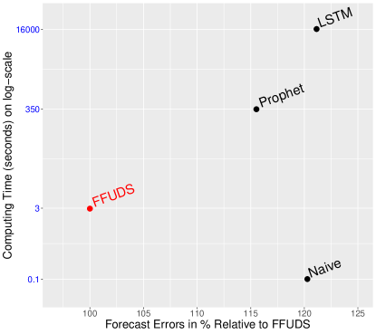
Figure 1: Performance of the new method. Notes: Forecast errors in percentages versus computing time in seconds (in blue) for the four forecasting methods: FFUDS (ours in red), LSTM, Prophet, and the naive method.

This paper makes several contributions. First, there is an emerging literature in information systems that takes a design science approach to solving forecasting problems in various business contexts. We extend this literature to a business context with high-frequency and unstable time series data for many geographical regions, by developing a novel, integral forecasting framework tailored towards the notable features of demand data for on-demand service platforms. The framework developed in this paper performs better than the popular approach in this literature that often uses some components of recurrent neural networks of the LSTM type (e.g., Liu et al.,, 2020, Wang et al.,, 2022, Wu et al.,, 2021).

Second, on-demand service platforms are typically subject to a changing environment due to factors such as expansion, competition, or external events; as a result, their demand data shows strong evidence of “change-points” which must be accounted for when forecasting demand. There is a recent literature in both economics and management on “forecast breakdown” and how to improve the forecasting ability of models in the presence of instabilities (see Rossi,, 2021 for a recent survey of this literature). This paper extends this literature by using a data-driven approach to detect breaks in forecast performance, leading to advantages such as offering a fast and scalable forecast procedure and alleviating the need to rely on human judgment to assess changing environments.

The rest of the paper is organized as follows. Section 2 reviews the relevant literature streams to which we contribute. Section 3 describes the platform demand data. Section 4 describes our proposed forecast framework FFUDS for streaming forecast breakdowns. Section 5 contains the empirical assessment of our approach to all UK delivery areas. Section 6 quantifies economic impact and discusses managerial insights of implementing an enhanced forecast procedure as FFUDS. Section 7 concludes and lays out future research directions.

2 Literature Review

This paper is related to several lines of research. First, there is a burgeoning literature in information systems that takes a design science approach to solving forecasting problems in various business scenarios, as described by Hevner et al., (2004). In this literature, recurrent neural networks for sequential data and in particular Long-Short-Term-Memory (LSTM) models have gained popularity in recent years. For instance, Wang et al., (2022) develops a deep learning model that combines LSTM components and embedding results to forecast passenger flows between pairs of city regions. LSTM models have been applied by Wu et al., (2021) to predict customer misbehavior in social media, by Liu et al., (2020) to identify useful solutions in online knowledge communities. LSTM models, however, require substantial computing time to estimate the model, even more so if hyper-parameter tuning is considered. Moreover, they do not account for breakdowns in forecast performance. As such, they are not tailored towards the above specificities of the forecast problem faced by on-demand service platforms operating in changing environments. This paper contributes to the information systems literature by developing a novel integral forecasting framework tailored towards the forecasting problem faced by on-demand service platforms.

In economics and management, there is a literature on how to detect forecast breakdowns and how to improve the forecasting ability of models in the presence of instabilities (see e.g., Rossi,, 2021 for a literature survey). Giacomini and Rossi, (2009) have pioneered the “forecast breakdown” research by proposing a breakdown test that requires the entire historic time series; however, such a method is not suitable in our streaming data setting in which only part of the time series is observable. More recently, one stream in this literature considers break/regime detection in the original time series (i.e., the demand data time series in our case). For instance, Killick et al., (2012), Fryzlewicz, (2014), and Chen et al., (2022) develop nonparametric change-point tests. Another stream in this literature studies break detection in the parameters modeling the dynamics in time series (see e.g., Dufays and Rombouts,, 2020). Finally, there are also papers such as Chib, (1998) that study Markovian dynamics that regulate the transition between breaks.

In the context of detecting breaks in steaming data, the Facebook Prophet method (Taylor and Letham,, 2018) forms an interesting benchmark method. It is a popular forecasting tool among practitioners that decomposes a time series into a trend, seasonal and holiday parts, handles out-of-sample forecast uncertainty, and in addition offers automatic change-point detection by including a sparse prior on the trend change parameter. These features require, however, Bayesian inference and thereby come at the cost of losing fast (closed-form) streaming estimators as desired in our case. Moreover, as opposed to parameter instability, we are particularly interested in detecting forecast breakdowns, so instability in the forecast performance as measured by a forecast error loss function over time.

We propose an innovative data-driven method to detect breaks in forecast performance. In the spirit of Pesaran and Timmermann, (2007), we combine the forecast based on the full-sample and the forecast based on the post-break estimation window. As such, break information is incorporated into the forecasts, while the full historical sample is utilized to stabilize the forecasts. Therefore, our forecasting framework is both accurate and fast-to-compute, tailored towards the streaming data setting of on-demand service platforms.

3 Data

We collaborate with Stuart, a leading on-demand delivery platform in Europe. We analyze UK demand data provided by this company at the hourly frequency from January 1, 2019 to March 31, 2021. Demand data are measured as the number of parcels to be delivered to 294 delivery areas it serves in the UK. To ease comparisons across areas, we assume that business operates everywhere on a daily basis between 9am and 11pm, which implies $T=12,315$ observations. In Figure 2, we visualize the hourly demand for Milton Keynes Central as an example of a delivery area. Figures 13, 14 and 15 in Appendix A provide additional insights into the demand heterogeneity across delivery areas.

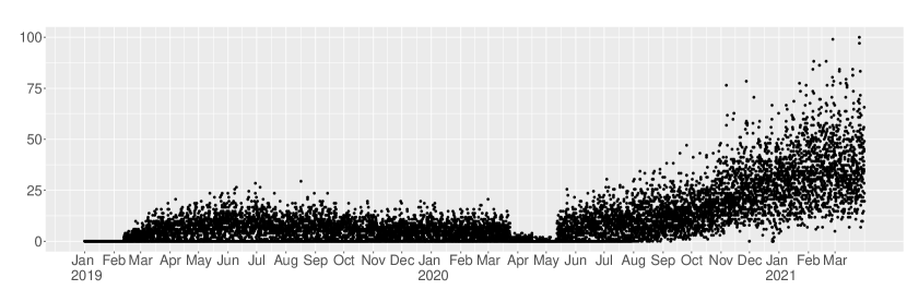
Figure 2: Hourly demand in Milton Keynes from January 1, 2019 until March 31, 2021.

Several distinctive features of this streaming data, representative for all delivery areas, appear. First, demand is highly unstable. In the first few months of 2019, demand grows gradually and then flattens until March 2020. The Covid-19 pandemic and first lockdown result in a huge demand drop for several weeks, but then demand quickly starts to grow at an exponential rate until the end of our sample. The pandemic has accelerated the growth of online shopping to unprecedented and unexpected levels. For instance, the United Nations Conference on Trade and Development (UNCTAD,, 2021) reports that global online retail sales’ share as part of total retail sales rose from 16% to 19% already in 2020. Second, the range of this demand data increases sharply over time. Hence, a modeling approach is needed that can swiftly adapt to these changes and their possibly unpredictable nature. Furthermore, strong intraday and day of the week seasonal demand patterns arise (see Figure 12 in Appendix A for more details). As these seasonal patterns vary across delivery areas, it is important to forecast demand at the area level which we do.

Next, we further investigate the instability in demand over the full sample period (2019-01-01 to 2021-03-31) to gain insights in the occurrence of structural changes (i.e. breaks). To this end, we employ a popular change-point detection method for each delivery area’s hourly demand series, namely the PELT nonparametric multiple change-point test Killick et al., (2012). Although the tests are retrospectively scanning the entire demand series for breaks, we get insights on the frequency and commonality of break dates which motivate the need for a demand forecast method that remains accurate in presence of breaks.

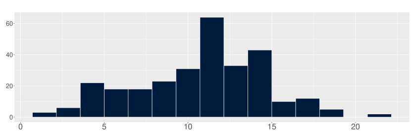
(a) Area count (vertical axis) of number of detected breaks (horizontal axis).

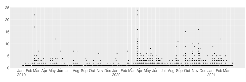
(b) Hourly time series plot of number of detected breaks summed over all areas.

Figure 3: Histogram (top) and time series (bottom) of the number of breaks (bottom) detected by PELT.

Figure 3(a) summarizes the number of detected breaks across delivery areas. On average about eleven breaks in each area are detected, though the range is large with some areas having hardly any break and one area having even 22 breaks. We next investigate the timing of the breaks dates and check if they cluster among delivery areas. Figure 3(b) plots the number of breaks detected hourly across all areas over the full sample period. We find at least one detected break in 15 percent of the day/hour date-stamps of the full sample. Breaks peak on March 22-23, 2020 where we count 181 detected breaks. This clearly points to the demand shifts related to the first Covid-19 lockdown. In addition, we find that between April, 2020 and March, 2021 systematically more breaks are detected than in the pre-Covid period. In fact, in this period, breaks affecting multiple delivery areas take place 35 percent of the time.

Demand in the post-Covid period differs considerably from that in the pre-Covid period. To illustrate this, we compute the daily average demand for the areas active before March 2020 (Pre-Covid) and still in business after May 2020 (Post-Covid). The results are displayed in Figure 4 with the 45 degree dashed line aiding to identify the directional change. Most areas see their demand being boosted to multiple times the pre-pandemic demand. A desirable property of a forecast model should therefore be a quick adaptation to a “new” regime. In the next section, we introduce our novel forecast method called “FFUDS” that enjoys these desirable properties.

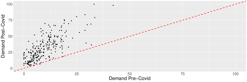
Figure 4: Scatterplot of pre- against post-Covid-19 average daily demand for all UK areas.

4 Model

The role of any data stream forecast system is to provide inputs for optimal decision making. In our particular case, the local decision maker at the delivery platform faces the following problem: every night, the upcoming fleet of required couriers needs to be planned using hourly demand forecasts for the next seven days. An automated procedure built by the central data science unit transfers these forecasts every night to all delivery areas. This procedure has to be quickly updated in case forecast performance deteriorates.

In Section 4.1 we discuss how we detect forecast breakdowns in data streams, in Section 4.2, we introduce our baseline demand model that we use to produce forecasts in a minimal amount of time. Both sections combined give rise to our Fast Forecasting of Unstable Data Streams (FFUDS) forecast framework. Next, in Section 4.3 we discuss our streaming forecast set-up and motivate our choice to use different forecast loss functions. In Section 4.4 we discuss the benchmark demand forecast models against which we compare FFUDS.

4.1 Streaming Forecast Breakdowns

We propose a procedure to detect instability in forecast performance since a sudden increase in forecast error loss signals the need to re-initiate the data set to estimate the model. In the following, in terms of notation, we denote the demand at hourly frequency for one specific delivery area as $d_{t}$ but note that our procedure is designed to apply to all areas simultaneously.

To test for a breakdown in forecast performance at daily frequency, define the forecast loss function on day $s>0$ for hourly horizon $h=1,\ldots,15$ as $L_{s}^{(h)}=L(d_{15(s-1)+h},d_{15(s-1)+h}^{f})$ with $d_{15(s-1)+h}^{f}$ denoting demand forecasts. The daily times series $\hat{L}_{s}^{(h)}$, having estimated $d_{15(s-1)+h}^{f}$, is used for online forecast breakdown detection. While in principle forecasts can be produced by any algorithm or model, for reasons outlined in the next section we take $d_{15(s-1)+h}^{f}=\mbox{E}(d_{15(s-1)+h}\mid I_{15(s-1)})$, where $\mbox{E}(\cdot\mid\cdot)$ is the conditional expectation operator and $I_{15(s-1)}$ the information set of available demand on day $s$ since the last break, if any.

We develop a new forecast breakdown procedure tailored towards the data streaming settings like the one at on-demand service platforms. In particular, we compute the daily time series $\hat{L}_{s}=\sum_{h=1}^{15}\hat{L}_{s}^{(h)}$ and build on the common approach in the change-point literature of detecting break dates through minimizing a cost function over possible numbers and locations of break dates. We use the computationally efficient Pruned Exact Linear Time (PELT) algorithm of Killick et al., (2012), available in the R (R Core Team,, 2022) package changepoint Killick and Eckley, (2014), with a normal likelihood test statistic that allows for changes in both mean and variance.

Once a forecast breakdown is detected, the question then arises how to adjust the demand forecast procedure. On the one hand, ignoring the detected break is likely to lead to inferior forecast performance at some point in time. On the other hand, using post-break data to produce forecasts is not always directly possible due to lack of data available after the detected break to estimate model parameters. In addition, especially in case of small breaks, there is large uncertainty to define the post break period. As documented for macroeconomic data by Marcellino et al., (2006) and Bauwens et al., (2015), incorporating breaks in the model does not lead uniformly to forecast gains, see Boot and Pick, (2020) for a recent theoretical discussion. In our case of hourly platform data, the number of breaks is typically higher than for macroeconomic series and their duration is quite heterogeneous. Given the uncertainty around the break dates and their size, using only data after an estimated break to estimate the model can yield worse forecasts than ignoring the breaks.

In between these two extremes, forecast combinations of full sample and post-break forecasts can be considered. Pesaran and Timmermann,, 2007 show that pooling forecasts from the same model but with different estimation windows, i.e. using both pre-break and post-break data, can improve out-of-sample forecast performance. To produce actual forecasts, Pesaran and Timmermann, (2007) use both weighted and simple average forecast combination. More general results on optimal forecasts and weighting schemes in presence of breaks can be found in Pesaran et al., (2013).

We use a forecast combination approach with equal weight to the full-sample forecast and post-break forecast. We opt for this approach mainly because of its simplicity, ease in implementation and its established track-record of good performance in the forecast combination literature (e.g., Elliott and Timmermann,, 2016, Chapter 14), but more elaborate schemes could be explored in future work. Concretely, we estimate the model parameters with the full historical sample and with the post-break sample, produce multi-step ahead forecasts for both and then average these for each horizon. If the post-break sample is too small to estimate the demand model, the full historical sample-based forecast gets all the weight until sufficient new post-break data has become available. In the next section, we introduce the demand model and how we estimate its parameters.

4.2 A Fast Baseline Demand Model

To employ our streaming forecast breakdown method, we require an approach to model and forecast demand data. Given our setup, a key feature that our demand model calls for is fast estimation. The model is used for optimal fleet planning on an hourly basis and has to be re-estimated at least daily for all areas. Based on the platform data characteristics from Section 3, we therefore propose a demand model whose parameter estimates can be obtained in closed-form, thus permitting real-time updates at large scale. In particular, we use the following parametric demand model:

$$d_{t}=\alpha_{0}+\sum_{j=1}^{M}\alpha_{j}t^{j}+\sum_{j=1}^{7}\gamma_{j}D_{jt}+\sum_{j=1}^{15}\left(\delta_{j}+\sum_{i=1}^{P}\phi_{i,j}d_{t-i}\right)H_{jt}+\varepsilon_{t},$$ (1)

with variables $D_{jt}=1$ if $d_{t}$ is on Day $j$ and 0 otherwise, $H_{jt}=1$ if $d_{t}$ is on Hour $j$ and 0 otherwise. The unknown parameters are the constant term $\alpha_{0}$, the trend parameters $\alpha_{j}$ ($j=1,\ldots,M$), the week-day parameters $\gamma_{j}$ ($j=1,\ldots,7$) , the hourly parameters $\delta_{j}$ ($j=1,\ldots,15$) and the autoregressive parameters $\phi_{i,j}$ (for hour $j$ at lag $i$); $\varepsilon_{t}$ is a zero mean white noise error term. The demand model allows for pronounced trend and seasonality features. Besides, although delivery areas share a similar overall pattern, they are bound to different effects because of their heterogeneous size and geographical location. We therefore use the same model specification for all areas, but allow for heterogeneity across areas by estimating the parameters separately.

Demand model (1) is potentially highly parameterized, which may impact its forecasting performance. For parameter identification purposes, we set $\alpha_{0}=\gamma_{1}=0$. To keep the model parsimonious, we incorporate domain-specific expertise from the delivery platform to impose several restrictions. Since mornings and evenings have different demand levels and therefore perhaps also dynamics, we set $\phi_{i,1}=\ldots=\phi_{i,4}$, $\phi_{i,5}=\ldots=\phi_{i,13}$ and $\phi_{i,14}=\phi_{i,15}$ to permit heterogeneity in the morning (9am-12pm), afternoon (1pm-9pm), and evening (10pm-11pm). We take a linear trend ($M=1$) because it empirically dominates a quadratic trend ($M=2$), set $P=105$ and use the following simple dynamics for the morning/afternoon/evening hours: for the morning hours, we include the demand from the same hour of the previous week ($d_{t-105}$). For the afternoon hours, we include the demand from the last hour ($d_{t-1}$), the demand from the same hour of the previous day ($d_{t-15}$) and the demand from the same hour of the previous week. For the evening hours, we include the demand from the last hour and the demand from the same hour of the previous week. The autoregressive parameters corresponding to all other lags are set to zero. Finally, including specific holiday effects or external data such as weather can easily be handled in this model. For example, December 25 (Christmas) and January 1st (New Year) are typically known for very low demand, and we handle such effects through dummy variables in the model.

Estimation of model (1) can be done using ordinary least squares (OLS). In fact, the model fits within the class of linear regression models and can be written in matrix form as $y=X\beta+\varepsilon$ with the closed form estimator $\hat{\beta}=\left(X^{\prime}X\right)^{-1}X^{\prime}y$ minimizing the squared Euclidean distance between $y$ and $X\beta$. In terms of notation, $y$ contains the to be forecast hourly demand, $X$ collects all predictors namely the deterministic components (trend and seasonal dummies) as well as the lagged demand values, and $\beta$ is the vector of all model parameters $\alpha$, $\gamma$, $\delta$ and $\phi_{ij}$.

To accommodate our streaming data setting, model (1) needs to be continuously re-estimated as new demand data becomes available, namely the 15 hourly demand series after each business day. To this end, we rely on renewable OLS estimation (Luo and Song,, 2020) which requires some additional notation to define the online estimator $\tilde{\beta}$. We denote $\tilde{\beta}_{1}=\hat{\beta}_{1}$ as the OLS estimator for model (1) given a first available sample of time points, and $\hat{\beta}_{b}=\left(X_{b}^{\prime}X_{b}\right)^{-1}X_{b}^{\prime}y_{b}$ as the OLS estimator for the same model on a new single data batch $D_{b}$. Then the renewable estimator based on historical data and incoming batches $b=2,3,\ldots$ can be written as

$$\tilde{\beta}_{b}=\left(\sum_{j=1}^{b-1}X_{j}^{\prime}X_{j}+X_{b}^{\prime}X_{b}\right)^{-1}\left(\sum_{j=1}^{b-1}X_{j}^{\prime}X_{j}\tilde{\beta}_{b-1}+X_{b}^{\prime}X_{b}\hat{\beta}_{b}\right).$$ (2)

In fact, the renewable estimator is equivalent to the Bayesian posterior updating formula for linear regression models with the cumulated historical ($j=1,\ldots,b-1$) information being the prior and $D_{b}$ the data. The size of $D_{b}$ can be different over time so that updated estimators can be computed independently from the frequency of $d_{t}$. In our specific case, we update every night using a new batch of 15 hourly demand observations obtained over the day. Thanks to its recursive updating scheme, such a streaming estimator reduces as much computing time as possible and requires only minimal amounts of data to be stored. Both aspects have direct measurable financial impact for platform businesses which typically operate via a cloud service provider such as Amazon Web Services (AWS) or Microsoft Azure. The renewable estimator above will, however, only work well in case of parameter stability and is therefore no substitute for the FFUDS approach. Next, we discuss the set-up of our streaming forecast exercise.

4.3 Set-Up and Loss Functions

We forecast hourly demand $d_{t}$ (from 9am to 11pm) at the end of every day for the next seven days, implying forecast horizon $h=1,\ldots,105$. This generates a daily stream of forecasts $d_{t}^{f}$ that can be evaluated against the actual demand the day after for $h=1,\ldots,15$, two days after for $h=16,\ldots,30$, etc. The resulting forecast loss functions can be used for (cumulative) performance tracking and detection of forecast breakdowns as explained in Section 4.1. We use several types of loss functions $L$. This allows gaining insights on the sensitivity of our approach with respect to the loss function, and painting a broader picture when comparing its performance against benchmarks. Figure 5 illustrates the differences between the considered loss functions. We now discuss the two statistical loss functions (Squared loss and Sape); the economic loss function, will be discussed in Section 6.1 on economic impact.

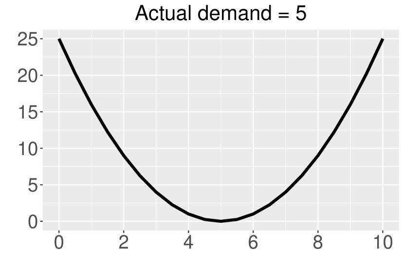
(a) Squared loss

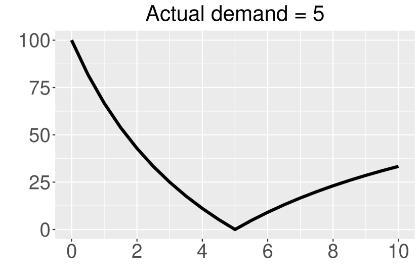
(b) Sape loss

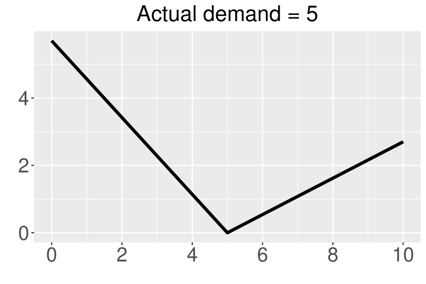
(c) Econ loss

Figure 5: Forecast error loss functions. Notes: Squared, sape and economic loss functions. On the x-axis are forecast values between 0 and 10. On the y-axis are the corresponding values of the respective loss functions for actual demands equal to five.

The first loss function is the classical squared error loss $L^{\mbox{sq}}(d_{t},d_{t}^{f})=(d_{t}-d_{t}^{f})^{2}$ which is symmetric and quadratically increasing away from $d_{t}$, see Figure 5(a). We use the root mean squared error (RMSE) which takes the square root of the average squared error losses when evaluating horizon specific forecasts. For evaluation of out-of-sample forecast accuracy, we average over $L^{\mbox{sq}}(d_{t},d_{t}^{f})$ losses across the different out-of-sample time points, take the square root and call this the RMSE loss function.

Secondly, we study the symmetric absolute percentage error loss $L^{\mbox{sape}}(d_{t},d_{t}^{f})=100\mid d_{t}-d_{t}^{f}\mid/(|d_{t}|+|d_{t}^{f}|)$, a popular metric used at delivery platforms due to its relative nature, thereby facilitating comparisons across delivery areas, and the fact that demand $d_{t}$ in small geographical areas can be zero making the standard absolute percentage error loss $L^{\mbox{ape}}(d_{t},d_{t}^{f})=100\mid(d_{t}-d_{t}^{f})/d_{t}\mid$ not defined. However, the $L^{\mbox{sape}}$ comes with its own peculiarities such as it being undefined when both actual and forecast demand are zero (i.e. perfect forecast setting), or its inability to differentiate forecast accuracy when actual demand is zero, then regardless of the value for $d_{t}^{f}$, a value of 100 is returned. When actual demand is non-zero, Figure 5(b) highlights the asymmetric shape of $L^{\mbox{sape}}$ (for the case of $d_{t}=5$). For evaluation of out-of-sample forecast accuracy, we average over $L^{\mbox{sape}}(d_{t},d_{t}^{f})$ losses across the different out-of-sample time points and call this the SMAPE loss function.

4.4 Benchmark Forecast Models

Finally, we compare the performance of our approach against several benchmarks. The first benchmark model is defined as $d_{t}=d_{t-105}+u_{t}$, with forecast $d^{f}_{t}=d_{t-105}$, which we call the “Naive” model since it implies that the forecast of a specific hour/day is the same value as observed in the previous week hour/day. An advantage of this specification is that it does not require parameter estimation, and it is expected to work well in the case of strong seasonality patterns as observed in our platform demand data.

The second benchmark is Facebook Prophet which implements automatic change-point detection in the parameters and is available in open-source software packages such as R (R Core Team,, 2022) and Python. We use the standard default prophet package in R (Taylor and Letham,, 2021). As a final benchmark, we use the popular Long-Short-Term-Memory (LSTM) network that we re-train at monthly frequency with fixed hyper-parameters throughout the forecasting exercise. We use the keras and tensorflow packages in R (Taylor and Letham,, 2021) in our applications. For a more detailed description on LSTM networks and the Prophet model, we refer to Appendix B.

We further highlight that, though simple at first sight, demand models should accurately capture trend and seasonal effects in the platform data, which is also the starting motivation for Prophet thereby making it a interesting benchmark. To illustrate this, in a preliminary analysis we construct a relatively short 30-day window that we update every night after having observed fifteen new hours of demand. We have 792 such windows between January, 2019 and March, 2021. Using these segments, we fit model (1) with $\phi_{ij}=0$, i.e. only trend and seasonality, for each of the delivery areas. Figure 6(a) shows the resulting rolling window average $R^{2}$s. Strikingly, trend and seasonality explains around 75% of average area demand variation in the beginning of 2019 but then increases oftentimes above 85% until the start of the first Covid-19 lockdown where the average $R^{2}$s drop temporarily back to about 80%. After this first lockdown, the average streaming $R^{2}$s gradually climb to new heights close to 95%. Capturing local trend and seasonality thus becomes increasingly more important towards the end of the sample and is expected to play the dominant role when modeling and forecasting area demand.

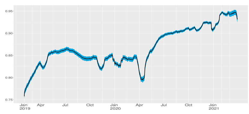
(a) R-squared

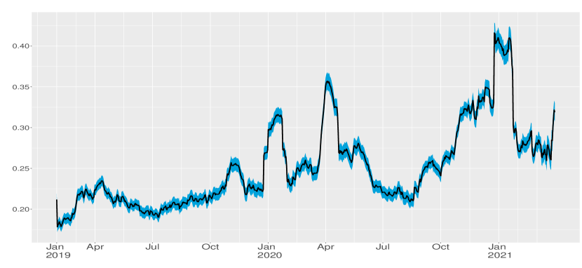
(b) First Order AutoCorrelation Coefficient

Figure 6: Streaming average $R^{2}$ (a) and First Order AutoCorrelation Coefficient (b) for the trend and seasonality model fitted to the delivery areas. One standard error bands are displayed in blue.

If so much variation is explained by trend and seasonality, what is left in terms of dynamic properties in the demand series? We investigate this by computing the amount of autoregressive dynamics after having filtered the trend and seasonality from the demand data. We compute a time series average, over the available delivery areas, of sample first order autocorrelation coefficients. Figure 6(b) reveals that, on average, the delivery areas filtered demand series have overall low autoregressive dynamics. At the start of the sample the average streaming sample autocorrelation coefficient hover around 20%, while they increase to just below 30% at the end of the sample in 2021. Nonetheless, some episodes are characterized by streaming sample autocorrelation coefficients up to 42%. While not being as strong as the trend and seasonal effects, it is therefore still worthwhile to study the presence of autoregressive dynamics in our streaming demand data setup. However, because we observe only short term memory effects, a full autoregressive moving average (ARMA) identification step seems unnecessary so that we can keep low the number of parameters driving autoregressive dynamics in the model.

In sum, demand is largely determined by trend and seasonal effects and little room is left to propose a richer model which exploits the subtle dynamics found in the data. Still, in the next section, we show that our FFUDS approach achieves sizable gains compared to the benchmarks.

5 Results

5.1 Results for All UK Delivery Areas

For all UK delivery areas, we implement a streaming exercise of our approach and benchmarks starting in February, 2019. Parameter estimates are updated, up to next-week-ahead forecasts are produced, forecast losses and next-business-day breakdown tests are implemented on a daily basis until March, 2021. We synthesize the streaming aspect by splitting the time span into pre-Covid and post-Covid periods, running respectively from February, 2019 to March, 2020 and April, 2020 to March 2021. In fact, the in-sample break detection tests reported in Section 3 evinced that after March, 2021 substantially more breaks appear in the delivery areas, making possible comparing our approach in a break-poor and break-rich scenario.

Table 1 summarizes over all delivery areas the SMAPE performance of our approach FFUDS against the three benchmarks. We zoom into the one-day-ahead forecast performance, i.e. one- to fifteen-hour-ahead forecasts, since they are in particularly used by the local area planners to decide on their next day operations, and they enter our forecast breakdown detection procedure. We display forecast errors in percentages relative to FFUDS. For instance, a relative forecast error of 120% indicates that the proposed method FFUDS performs 20% better than the benchmark method.

Table 1: SMAPE forecast performance. Notes: One-day-ahead SMAPE forecast performance of the forecast methods FFUDS, Naive, Prophet and LSTM relative to the proposed method FFUDS, averaged across all delivery areas. Values above 100 indicate the percentage gain in forecast accuracy of FFUDS relative to the benchmark.

						Pre-Covid							Post-Covid
Hours					FFUDS	Naive	Prophet	LSTM				FFUDS	Naive	Prophet	LSTM
All					100.00	125.20	103.68	111.38				100.00	120.28	115.53	121.14

We first examine the pre-Covid period, the relatively calmer period with few disruptions. The proposed FFUDS considerably outperforms the naive model, with an overall gain of 25%. Even a relatively calm period for the platform data requires more than just capturing seasonality effects. The more advanced Prophet package performs better than the naive benchmark across all hours of the day, though our FFUDS approach dominates with an overall gain of 3%. Finally, the LSTM neural network is outperformed by 11% by our FFUDS approach in the pre-Covid period.

Post-Covid period wise, i.e. the period from April 2020 onward, the results are even more in favor of our approach. FFUDS strongly dominates the three benchmarks. In fact, Prophet is now outperformed with 15% compared to 3% pre-Covid. LSTM, ignorant to the presence of breaks, becomes less competitive to FFUDS in the post-Covid period which is characterized by more disruptions and is therefore outperformed by 21%. Overall, we can conclude that the proposed FFUDS approach systematically yields better forecasts than the benchmarks.

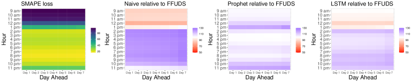
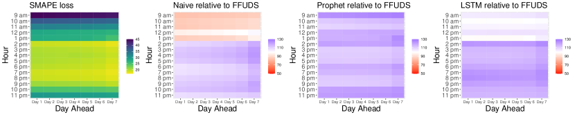
Figure 7: SMAPE forecast performance heat maps. Notes: Heat maps of SMAPE forecast performance averaged across delivery areas for different hours of day (vertical axis) and days-ahead (horizontal axis). Top: Pre-Covid. Bottom: Post-Covid. Column one: Loss for FFUDS. Column two, three, four: Respectively Naive, Prophet and LSTM relative to FFUDS. Values above (below) 100% visualized in blue (red) indicate better (worse) performance of the proposed method FFUDS compared to benchmark. Equal performance is visualized in white.

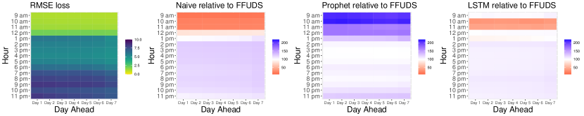
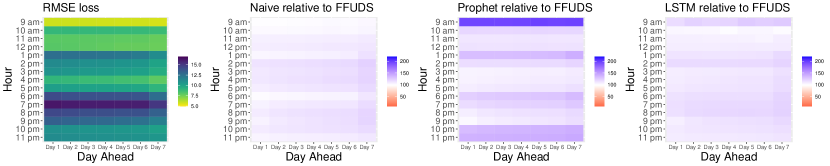
Figure 16: RMSE forecast performance heat maps. Notes: Heat maps of RMSE forecast performance averaged across delivery areas for different hours of day (vertical axis) and days-ahead (horizontal axis). Top: Pre-Covid. Bottom: Post-Covid. Column one: Loss for FFUDS. Column two, three, four: Respectively Naive, Prophet and LSTM relative to FFUDS. Values above (below) 100% visualized in blue (red) indicate better (worse) performance of the proposed method FFUDS compared to benchmark. Equal performance is visualized in white.

Figure 7 provides more disaggregated details about the forecast performance per hour over the seven-day horizon for respectively the pre-Covid (top) and post-Covid (bottom) periods. As before, we use the SMAPE loss function, results on the RMSE loss are available in Figure 16 of Appendix C. It turns out that forecast capacity depends more on the time of day rather than the day-ahead. For example, forecasting 4pm area demand on Day 1 is almost as easy as forecasting 4pm demand on Day 7. The same is true for other business hours. These intraday figures re-emphasize that overall FFUDS largely dominates both in pre- and post-Covid periods. They also show that in the pre-Covid period morning hours are difficult to forecast as indicated by the orange lines. The main reason for this is the systematically recurring close to zero morning demand. In the post-Covid period, our FFUDS approach performs better in this part of the day. This can also be seen in the left column of Figure 7 which quantify for our FFUDS approach the forecast loss in absolute levels per hour over the seven-day horizon. Indeed, the largest values of the SMAPE loss function decrease for the post-Covid period from 80 to 45 percent in this second period of our sample.

5.2 Case Study: Wimbledon

After studying all UK delivery areas together, we focus on one representative area in London, namely Wimbledon, to have a clearer view on where FFUDS finds breaks and how it performs throughout the 2019-2021 sample period.

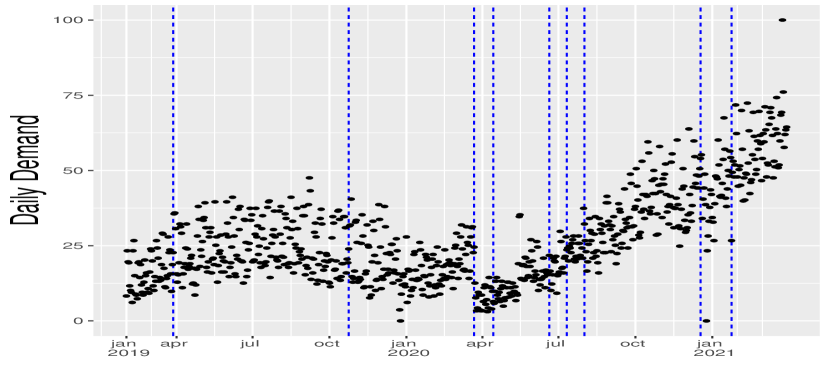
(a) Daily demand

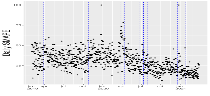
(b) Daily forecast accuracy

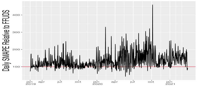
(c) Forecast accuracy Prophet versus FFUDS

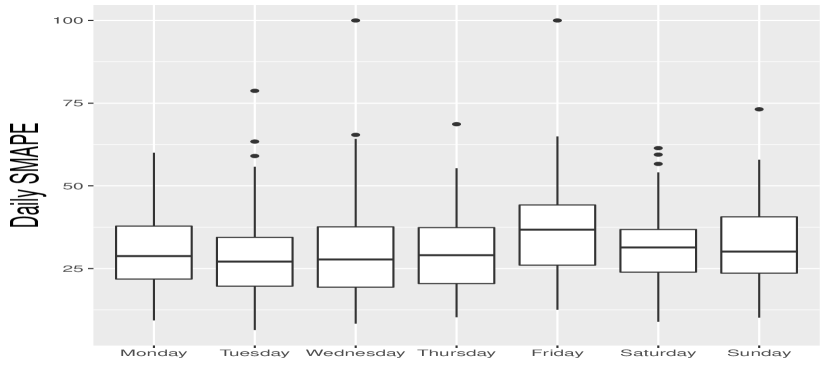
(d) Day of the week forecast accuracy

Figure 8: Wimbledon results.

Figure 8 presents the streaming results for Wimbledon. Figure 8(a) shows demand aggregated to a daily frequency. We clearly see the changes in the local growth patterns, the impact of the Covid-19 first lockdown and the subsequent strong and almost linear growth. The vertical dashed blue lines indicate the nine breaks detected by FFUDS on the streaming SMAPE loss as displayed in Figure 8(b). In fact, the implied break dates from SMAPE loss exhibit clear changes in forecast loss for most changes, especially towards the end of the sample where SMAPE reaches levels between 10-30% compared to 20-60% before Covid-19. Figure 8(c) highlights the streaming relative performance of FFUDS compared to Prophet, the platform’s current forecast method, by simply dividing the respective daily losses over the sample period. In favor of FFUDS, the ratio is above 100% (red line) in extended periods, especially since July 2020. For some specific days, Prophet dominates.

In the previous section, the general results across forecast horizons (over all delivery areas) reveal that forecast accuracy changes most throughout the business day, with small performance differences between next day and further remote weekdays. For Wimbledon, we also look at differences in forecast accuracy over the specific days of the week. Figure 8(d) shows boxplots of SMAPE forecast accuracy from Monday until Sunday. Except for Fridays where the median performance is slightly worse, probably due to higher volume and weekend start effects like non-regular sales, forecast performance is stable across days of the week.

6 Implications

The natural question to ask next is how the enhanced predictive performance of our approach translates in economic gains (Section 6.1) and managerial insights (Section 6.2).

6.1 Economic Impacts

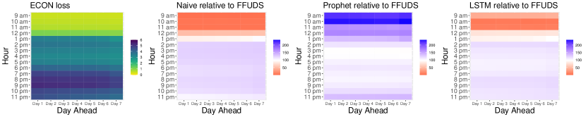
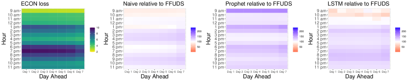
Figure 17: ECON forecast performance heat maps. Notes: Heat maps of ECON forecast performance averaged across delivery areas for different hours of day (vertical axis) and days-ahead (horizontal axis). Top: Pre-Covid. Bottom: Post-Covid. Column one: Loss for FFUDS. Column two, three, four: Respectively Naive, Prophet and LSTM relative to FFUDS. Values above (below) 100% visualized in blue (red) indicate better (worse) performance of the proposed method FFUDS compared to benchmark. Equal performance is visualized in white.

We investigate the economic impact of FFUDS’s superior forecast performance. First, we quantify monetary impact. While the above discussed loss functions are traditional “statistical” choices measuring how far the forecast is from its realization, we now convert forecasts into a business-relevant money implied metric. Such a metric reflects the company’s business operations and strategy, and is therefore by construction company specific. Based on information from Stuart, the monetary loss function we use is measured in British Pounds and given by $L^{\mbox{econ}}(d_{t},d_{t}^{f})=1.14(d_{t}-d_{t}^{f})\mathds{1}_{{d_{t}>d_{t}^{f}}}+0.54(d_{t}^{f}-d_{t})\mathds{1}_{{d_{t}^{f}>d_{t}}}$ where $\mathds{1}_{{(\cdot)}}$ denotes the indicator function. When forecast/planned demand is lower than actual demand, independent couriers are not always available to handle the extra deliveries and business opportunities are missed. A relatively high cost of is associated to this circumstance. In the opposite situation, when forecast/planned demand exceeds actual demand, couriers are potentially paid without having to deliver. The platform evaluates this situation as less costly than the former. The economic loss function is thus asymmetric as illustrated in the right panel of Figure 5. Table 2 is the economic analogue of Table 1 summarizing economic forecast performance. Figure 17 in Appendix C is the economic heat map analogue of Figure 7.

Also in terms of economic forecast performance, FFUDS largely dominates the other benchmark models. To summarize monetary impact, we sum these hour/day specific area monetary losses over 2021-Q1, the last available quarter. Doing this for FFUDS and comparing to the three benchmark methods gives the yearly gains (in UK pounds) displayed in the bottom row of Table 2. Compared to the best performing benchmark, namely the LSTM model, we obtain a striking £1,583,956 gain on a yearly basis. The gains over the other two benchmarks are even larger. Hence, while the statistically measured relative forecast performance against the best benchmark is only a few percentage points, which might appear small at first sight, the economic gains add up considerably.

Table 2: Economic forecast performance. Notes: One-day-ahead economic forecast performance of the forecast methods FFUDS, Naive, Prophet and LSTM, relative to the proposed method FFUDS, across all delivery areas. Values above 100 indicate the percentage gain in forecast accuracy of FFUDS relative to the benchmark. The bottom row summarizes the yearly gain of FFUDS over the three benchmarks in UK Pounds.

Period				FFUDS		Naive		Prophet		LSTM
Pre-Covid				100.00		130.15		120.87		116.46
Post-Covid				100.00		127.07		130.60		123.53
Yearly gain FFUDS (in UK Pounds)				-		1,604,324		3,070,548		1,583,956

Second, we investigate computational cost of our procedure FFUDS compared to the benchmark methods Prophet and LSTM. We measure computing time as the number of seconds it takes to do one daily update of estimating and then forecasting a full week-ahead of hourly demand for all UK areas. Because the sample size is largely different in the beginning of 2019 than at the end of our sample (March, 2021), we measure computing time on both. Table 3 reports computing times (in seconds) on a Microsoft Windows 11 Pro with 16-core AMD Ryzen Threadripper PRO i5 4,3 GHz processor.

For the short sample, FFUDS is roughly 120 times faster than Prophet, and even more than 5,500 times faster than LSTM. For the long sample, FFUDS is a stunning 220 and 27,000 times faster than respectively Prophet and LSTM. LSTM requires over 200 hours computing time across all delivery areas, hence forecasting over-night at the end of the sample is simply impossible in practice (unless parallel programming is used).

These results imply that higher frequency than daily forecast updates, which are becoming increasingly required for on-demand platforms, can become compromisingly slow for Prophet and LSTM, or other packages based on sampling methods. In contrast, our procedure FFUDS estimates and forecasts all areas in less than a minute. This speed is also strategically important because platforms are nowadays challenged on their carbon footprints due to the running of computationally intense algorithms. Importantly, FFUDS’s drastic reduction in computing time does not come at a cost in terms of estimation accuracy. Indeed, Figure 1 summarizes the computing time (vertical axis) and forecast errors (SMAPE, horizontal axis) of the four methods. FFUDS is the only method placed at the bottom left, thereby combining low computing time with high prediction accuracy.

Table 3: Computational metrics. Notes: Computing time (in seconds on a Microsoft Windows 11 Pro with 16-core AMD Ryzen Threadripper PRO i5 4,3 GHz processor) and costs (in US dollars) for FFUDS, and benchmarks Prophet and LSTM.

			Computing Time (seconds)							Computing Costs (US dollars)
	Sample		FFUDS		Prophet		LSTM			FFUDS		Prophet		LSTM
	Short		2.94		346.87		16,287.73			0.13		15.05		706.797
	Long		26.31		5,912.03		725,209.1			1.14		256.55		31,470.05

Finally, beyond the strategically important new services that can be offered to customers and drivers, the speed of our procedure has also direct financial consequences. To illustrate this, we take the example of cloud computing costs. An AWS m5.2xlarge EC2 instance costs at the time of writing approximately 0.428 US Dollar ($) per hour. Table 3 summarizes the yearly costs (in US Dollars) of FFUDS, Prophet and LSTM for forecasts updates done all year around. Yearly costs are drastically lower for FFUDS than for the benchmark methods, especially LSTM. In case of the long estimation sample, for instance, the difference becomes a striking $1.14 for FFUDS compared to $31,470 for LSTM. Note that these costs increase linearly with the number of delivery areas within a given country, and that most on-demand platforms operate internationally.

6.2 Managerial Insights

Opening new delivery areas, merging or splitting existing ones, is together with expected market growth of strategic importance for any on-demand delivery platform. In fact, local demand forecasting accuracy impacts the supply of drivers and their compensation, speed of delivery and therefore customer satisfaction. Figure 9 sheds light on the relationship between market share, market size, market growth for FFUDS’s SMAPE loss function at the delivery area level. Market growth is defined as the ratio of a delivery area’s demand from the last available quarter relative to demand from the first available quarter. Market share of a delivery area is defined as the ratio of total demand of the area relative to total UK demand in 2021-Q1.

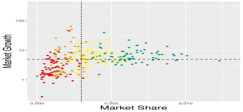
(a) Market share - Market growth

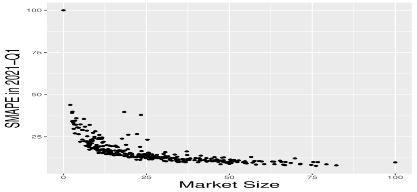
(b) Market size - Forecast accuracy

Figure 9: Performance of the new approach related to market characteristics.

Figure 9 panel (a) displays on a market share - market growth log-scale the SMAPE performance of all areas. The dashed lines indicate the median levels of market share and growth, and we group by quartiles the SMAPE losses decreasing from red (worst), orange, yellow to green (best). The left lower quadrant, containing relatively small and no growth areas turn out to be the most complicated to forecast demand for. Performance improves somewhat for small areas with large market growth, see the left top quadrant. The picture turns yellow and mostly green in the two right quadrants, which constitute larger areas that typically grow between four and twenty percent.

Figure 9 panel (b) emphasizes the effect of delivery area size on forecast performance. Smaller areas are difficult to forecast relative to larger ones. However, this relationship is not linear and the gains of increasing the size of the areas taper off after levels of 30 in terms of total Q1-2021 demand. This finding is important because very large areas are less straightforward to manage in terms of supply and pricing strategies. Areas that grow too large can therefore be re-organized without loss of demand forecast accuracy. On the other hand, forecasting-wise opening new areas that suffer from initial low demand makes sense only if rapid growth is expected.

Another strategically important issue for delivery platforms is scale, requiring wide market coverage to have a large enough volume to cover fixed costs, but also for example to strike deals with nationwide chains. Consequently, understanding the geographical differences in terms of operational efficiency allows prioritizing where to expand. We analyze the forecast performance of FFUDS for all UK delivery areas and look into differences between small and large city regions. Overall, we find that smaller cities with a small amount of delivery areas are more complicated to forecast than larger cities. Figures 11 and 11 illustrate this for the London and Newcastle regions. The size of the circles reflect the size of the SMAPE loss in 2021-Q1. The London region with many delivery areas outperforms Newcastle on average, though one can also see areas in the city center of London that are not that easy to forecast either which might be due to fierce local competition or volatile demand.

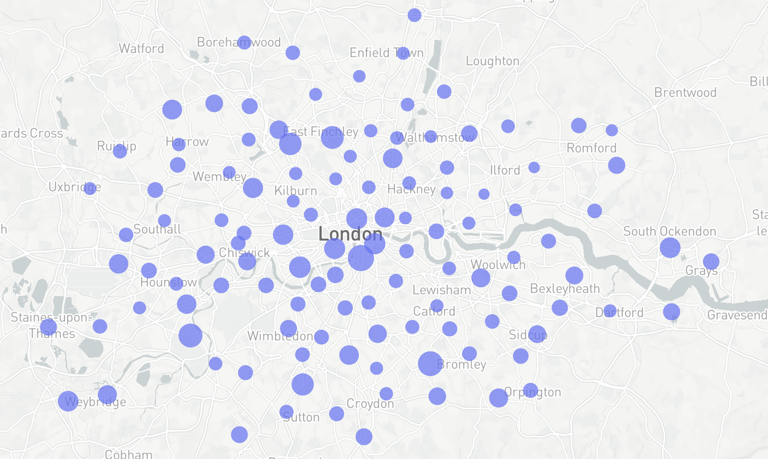
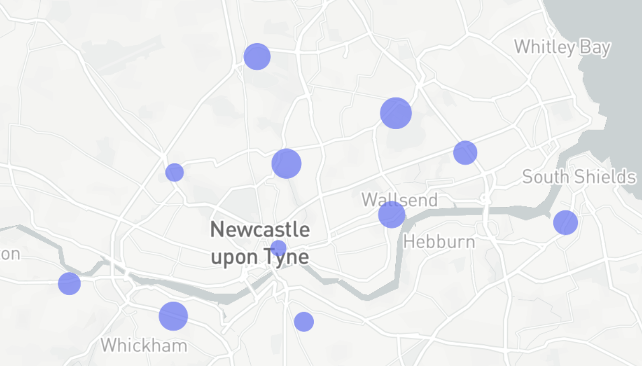
Figure 10: London region SMAPE loss; the larger the circle the larger the loss.

Figure 11: Newcastle region SMAPE loss; the larger the circle the larger the loss.

7 Conclusion

On-demand service platforms are subject to irregular growth. Keeping them operationally efficient is challenging because such data-driven platforms require forecasting at a large scale for decision making. A successful forecast framework must be adaptive to rapidly changing environments, yet because of scale, can typically use own historical data only. Since platform data is streaming and forecasts need to be produced at high-frequency, the approach has to be computationally fast.

A careful examination of platform data characteristics, reveals that, while strong trend and seasonality effects are present, the data streams are heavily impacted by episodes of instability. Therefore, we build Fast Forecasting of Unstable Data Streams (FFUDS), an automated framework that uses historical data and rests on two key components. First, the use of a break detection procedure on streaming forecast losses, which allows dynamically adapting the data weighting scheme used for forecasting. Second, the development of a new model that incorporates seasonality, trends, and nonlinear dynamic effects, that is simple enough to estimate in closed-form thereby permitting a fast streaming data setting. We empirically validate our approach using demand from all UK delivery areas from an on-demand delivery platform, find it to outperform several industry benchmarks, and analyze the strong positive economic and managerial implications of such enhanced forecast performance. Our approach is computationally fast so that it permits efficient forecast updates when new data becomes available, and it is applicable in the large-scale multi-country setting in which platforms typically operate.

Future research will be devoted to geospatial modeling of delivery areas, and the inclusion of supply data of the independent couriers to handle further automation of prescriptive decision making regarding pricing. Of particular interest is surge pricing which platforms use as a signaling device by increasing a worker’s compensation at a given delivery area above the regular price of the entire market place to balance demand and supply in areas with a shortage of workers compared to the demand, see e.g., Guda and Subramanian, (2019) and Garg and Nazerzadeh, (2022) for more details. Another topic on our agenda when considering both demand and supply data is explicitly incorporating the objective function and constraints regarding the optimal decision problem into the estimation problem, along the lines recently provided by Elmachtoub and Grigas, (2022).

The framework we develop has been successfully applied to a on-demand delivery platform, but generalises to any other business setting that encounters unstable data streams. For instance, it has also been applied to the forecasting of hourly consumer traffic at thousands of offline stores of a large technology company. We can think, for example, of hospitality platforms that deliver hotel occupation rate forecasts to their clients for the optimisation of hotel personnel, food and leisure activities, but that face issues of suddenly changing COVID-19 restrictions or of geopolitical events.

Acknowledgements. We are very grateful to Benjamin Wolter for expert advice, to Arnaud Dufays, Sarah Gelper, Harris Kyriakou, Olivier Scaillet for comments and checks provided on earlier versions of the paper and to the participants at the Symposium on Statistical Challenges in Electronic Commerce Research (SCECR 2022), the Conference on Data Science, Statistics & Visualisation (DSSV 2022), the International Symposium on Forecasting (ISF 2022), and the Workshop on Information Technologies and Systems (WITS 2022) for helpful discussions. IW was financially supported by the Dutch Research Council (NWO) under grant number VI.Vidi.211.032.

Appendix A Data Description: Additional Insights

We provide additional insights into the (i) seasonality of the demand data, and (ii) demand heterogeneity across delivery areas.

Figure 12(a) shows intraday UK demand. While demand is aggregated over all product categories (food, fashion, health, etc.), the large majority of deliveries consists of food. This explains why demand starts low at 9am, is moderately high around lunchtime (12-2pm), goes down only mildly between 2-5pm, sharply increases afterwards and peaks around 8pm, after which it decreases again to levels comparable to late afternoon. Apart from a strong intraday demand pattern, pronounced day of the week fluctuations are present as well, see Figure 12(b). Average demand is lowest on Mondays, steadily increases until Thursdays, jumps on Fridays and Saturdays, and lowers on Sundays. These intra-day and weekly demand patterns also arise for the delivery areas albeit some areas have no reduction in late afternoon demand, or peak later than 8pm.

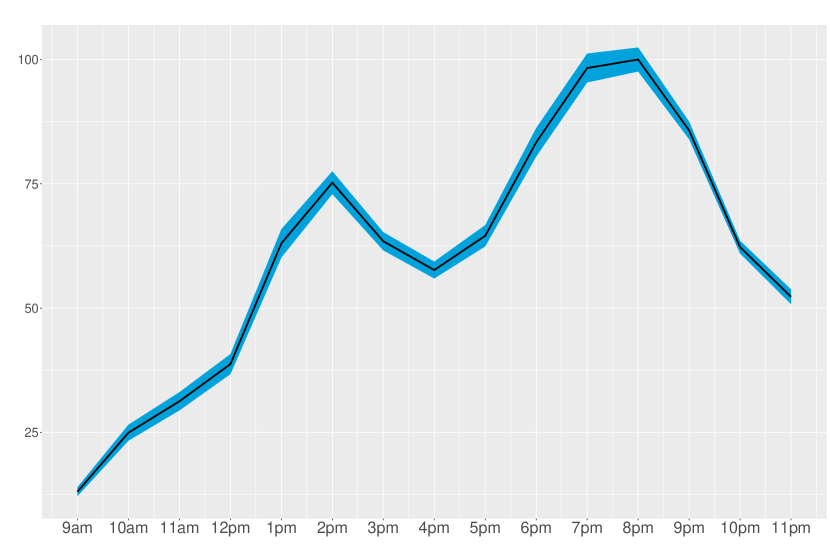
(a) Intraday Demand

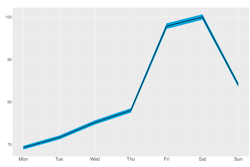
(b) Day of Week Demand

Figure 12: Intraday hourly demand and day of the week average demand for UK. One standard error bands are displayed in blue.

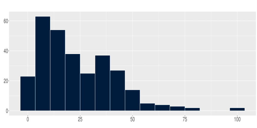
Figure 13: Histogram for aggregated demand in each delivery area of the UK.

Figure 13 shows the histogram of total demand for the delivery areas over the entire sample period. An interesting tri-modal pattern emerges. The first and largest group has total demand of less than 25, the second largest group up to 50. A small third group has high demand of almost 100, the largest delivery area being Bethnal Green in the London region. Figure 14 visualizes the demand on a UK map to highlight the geographical coverage of the delivery areas. Each circle is placed at the center of one out of the 294 areas, giving by its latitude and longitude, and its diameter is proportional to the area’s total demand. Unsurprisingly, most cities are covered with multiple delivery areas, the number of which is directly related to population size. Figure 15 zooms in on the London area and reveals that the delivery area total demand is not uniformly distributed. The main reason for this is that fleet planning is organized with respect to drivers’ availability rather than clients’ demand, thereby giving rise to substantial area-demand heterogeneity ranging from housing over business towards tourist areas.

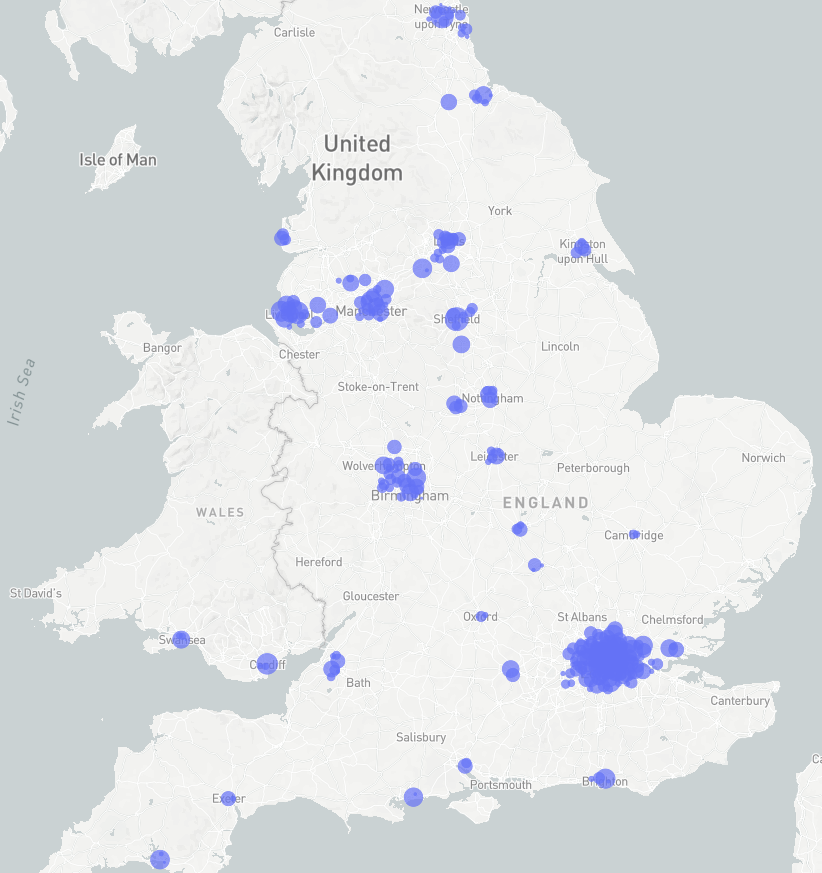
Figure 14: Aggregated demand in each delivery area in the UK.

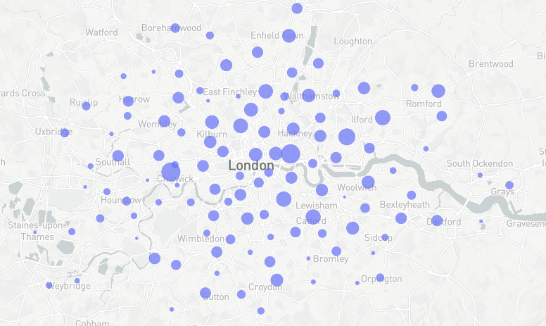
Figure 15: Aggregated demand in each delivery area in the London region.

Appendix B Prophet and LSTM Benchmarks

We provide a brief description of the Prophet and LSTM forecasting approaches. We denote the demand at hourly frequency for one specific delivery area as $d_{t}$. Both approaches rely on historical information up to time $t$ to forecast $d_{t+h}$ where $h$ is the forecast horizon.

B.1 Prophet

The main idea behind Prophet is decomposing $d_{t}$ into the following three deterministic parts:

$$d_{t}=g_{t}+s_{t}+v_{t}+\varepsilon_{t}$$ (3)

with $g_{t}$ the trend, $s_{t}$ and $v_{t}$ the seasonal and holiday parts respectively. The zero mean error term $\varepsilon_{t}$ represents idiosyncratic changes not captured by the three parts. The advantage of this deterministic approach is that the forecast for $d_{t+h}$ can be directly computed as $g_{t+h}+s_{t+h}+v_{t+h}$. The trend part $g_{t}$ is specified by a flexible piece-wise logistic growth model accounting for change-points in the time series at known (specified by the user) or unknown dates (determined by the data only). Growth rate, capacity and offset parameters drive this trend specification. The seasonal part $s_{t}$ is captured by a standard Fourier series yielding smooth effects, and for which parameter coefficients need to be estimated. Finally, holiday effects $v_{t}$ are typically unsmooth and are therefore integrated in the model using indicator functions each of which are multiplied by a parameter representing the specific average effect. Assuming a law for $\varepsilon_{t}$, e.g. Gaussian, the likelihood of model (3) is known and is then combined with uninformative priors for posterior inference on the parameters. This allows integrating model parameter uncertainty and can take care of out-of-sample forecast uncertainty, but these features require additional computation time. See Taylor and Letham, (2018) for more detailed explanations.

B.2 LSTM Neural Network

Long-Short-Term-Memory (LSTM) networks were first introduced by Hochreiter and Schmidhuber, (1997), and have become increasingly popular for time series forecasting. They are part of recurrent neural networks but they do not suffer from the vanishing/exploding gradient problem that arises when minimising the forecast error loss function. An LSTM filters information through an input ($i_{t}$), forget ($f_{t}$), output ($o_{t}$) gate. The forget gate ensures that the input and output gates consider only the important information of the new input and previous time period respectively. A cell state $c_{t}$ introduces some memory to the LSTM in order to remember the past. More formally, the structure of an LSTM to forecast $d_{t+h}$ is a follows:

$$i_{t} = \sigma\left(W_{i}X_{t}+U_{i}h_{t-1}+b_{i}\right)$$

$$f_{t} = \sigma\left(W_{f}X_{t}+U_{f}h_{t-1}+b_{f}\right)$$

$$o_{t} = \sigma\left(W_{o}X_{t}+U_{o}h_{t-1}+b_{0}\right)$$

$$c_{t} = f_{t}\odot c_{t-1}+i_{t}\odot\tanh\left(W_{c}X_{t}+U_{c}h_{t-1}+b_{c}\right)$$

$$h_{t} = o_{t}\odot\tanh(c_{t})$$

$$\hat{d}_{t+h} = W_{d}h_{t}+b_{d}$$

where the weight matrices $W$, $U$, and bias vectors $b$ contain the parameters to be estimated, $X_{t}$ is the historical demand data, $\sigma$ is the sigmoid function, $\odot$ is the element-wise (or Hadamard) product operator. The number of units in the LSTM is for example reflected by the dimension of the input function $i_{t}$. The initial cell state $c_{0}$ and hidden state $h_{0}$ are set to zero. Stochastic gradient descend methods are employed to minimise the squared loss $\Sigma_{t}(d_{t+h}-\hat{d}_{t+h})^{2}$ summed over the available demand data.

Appendix C Forecast Performance: Additional Results

Table 4: RMSE forecast performance. Notes: One-day-ahead RMSE forecast performance of the forecast methods FFUDS, Naive, Prophet and LSTM relative to the proposed method FFUDS, averaged across all delivery areas. Values above 100 indicate the percentage gain in forecast accuracy of FFUDS relative to the benchmark.

						Pre-Covid							Post-Covid
Hours					FFUDS	Naive	Prophet	LSTM				FFUDS	Naive	Prophet	LSTM
All					100.00	128.54	107.74	110.99				100.00	119.07	138.68	116.23

References

- Abhishek et al., (2021) Abhishek, V., Dogan, M., and Jacquillat, A. (2021). Strategic timing and dynamic pricing for online resource allocation. Management Science, 67(8):4880–4907.
- Barrios et al., (2022) Barrios, J. M., Hochberg, Y. V., and Yi, H. (2022). Launching with a parachute: The gig economy and new business formation. Journal of Financial Economics, 144(1):22–43.
- Bauwens et al., (2015) Bauwens, L., Koop, G., Korobilis, D., and Rombouts, J. (2015). The contribution of structural break models to forecasting macroeconomic series. Journal of Applied Econometrics, 30(4):596–620.
- Boot and Pick, (2020) Boot, T. and Pick, A. (2020). Does modeling a structural break improve forecast accuracy? Journal of Econometrics, 215(1):35–59.
- Chen et al., (2019) Chen, M. K., Chevalier, J. A., Rossi, P. E., and Oehlsen, E. (2019). The value of flexible work: Evidence from uber drivers. Journal of Political Economy, 127(6):2735–2794.
- Chen et al., (2022) Chen, Y., Wang, T., and Samworth, R. J. (2022). High-dimensional, multiscale online changepoint detection. Journal of the Royal Statistical Society: Series B (Statistical Methodology), 84(1):234–266.
- Chib, (1998) Chib, S. (1998). Estimation and comparison of multiple change-point models. Journal of Econometrics, 86:221–241.
- Dufays and Rombouts, (2020) Dufays, A. and Rombouts, J. V. (2020). Relevant parameter changes in structural break models. Journal of Econometrics, 217(1):46–78.
- Elliott and Timmermann, (2016) Elliott, G. and Timmermann, A. (2016). Economic Forecasting. Princeton University Press, Princeton, New Jersey.
- Elmachtoub and Grigas, (2022) Elmachtoub, A. N. and Grigas, P. (2022). Smart “predict, then optimize”. Management Science, 68(1):9–26.
- Fryzlewicz, (2014) Fryzlewicz, P. (2014). Wild binary segmentation for multiple change-point detection. The Annals of Statistics, 42(6):2243–2281.
- Garg and Nazerzadeh, (2022) Garg, N. and Nazerzadeh, H. (2022). Driver surge pricing. Management Science, 68(5):3219–3235.
- Giacomini and Rossi, (2009) Giacomini, R. and Rossi, B. (2009). Detecting and Predicting Forecast Breakdowns. The Review of Economic Studies, 76(2):669–705.
- Guda and Subramanian, (2019) Guda, H. and Subramanian, U. (2019). Your uber is arriving: Managing on-demand workers through surge pricing, forecast communication, and worker incentives. Management Science, 65(5):1995–2014.
- Hevner et al., (2004) Hevner, A., March, S., Park, J., and Ram, S. (2004). Design science in information systems research. Management Information Systems Quarterly, 28(1):75–105.
- Hochreiter and Schmidhuber, (1997) Hochreiter, S. and Schmidhuber, J. (1997). Long Short-Term Memory. Neural Computation, 9(8):1735–1780.
- Killick and Eckley, (2014) Killick, R. and Eckley, I. (2014). changepoint: An R package for changepoint analysis. Journal of statistical software, 58(3):1–19.
- Killick et al., (2012) Killick, R., Fearnhead, P., and Eckley, I. A. (2012). Optimal detection of changepoints with a linear computational cost. Journal of the American Statistical Association, 107(500):1590–1598.
- Kremer et al., (2011) Kremer, M., Moritz, B., and Siemsen, E. (2011). Demand forecasting behavior: System neglect and change detection. Management Science, 57(10):1827–1843.
- Liu et al., (2021) Liu, S., He, L., and Shen, M. Z.-J. (2021). On-time last-mile delivery: Order assignment with travel-time predictors. Management Science, 67(7):4095–4119.
- Liu et al., (2020) Liu, X., Wang, G. A., Fan, W., and Zhang, Z. (2020). Finding useful solutions in online knowledge communities: A theory-driven design and multilevel analysis. Information Systems Research, 31(3):731–752.
- Luo and Song, (2020) Luo, L. and Song, P. X.-K. (2020). Renewable estimation and incremental inference in generalized linear models with streaming data sets. Journal of the Royal Statistical Society: Series B (Statistical Methodology), 82(1):69–97.
- Marcellino et al., (2006) Marcellino, M., Stock, J. H., and Watson, M. W. (2006). A comparison of direct and iterated multistep ar methods for forecasting macroeconomic time series. Journal of Econometrics, 135:499–526.
- Parker and Van Alstyne, (2005) Parker, G. G. and Van Alstyne, M. W. (2005). Two-sided network effects: A theory of information product design. Management Science, 51(10):1494–1504.
- Pesaran et al., (2013) Pesaran, M. H., Pick, A., and Pranovich, M. (2013). Optimal forecasts in the presence of structural breaks. Journal of Econometrics, 177(2):134–152.
- Pesaran and Timmermann, (2007) Pesaran, M. H. and Timmermann, A. (2007). Selection of estimation window in the presence of breaks. Journal of Econometrics, 137(1):134–161.
- R Core Team, (2022) R Core Team (2022). R: A Language and Environment for Statistical Computing. R Foundation for Statistical Computing, Vienna, Austria.
- Rochet and Tirole, (2003) Rochet, J.-C. and Tirole, J. (2003). Platform Competition in Two-Sided Markets. Journal of the European Economic Association, 1(4):990–1029.
- Rossi, (2021) Rossi, B. (2021). Forecasting in the presence of instabilities: How do we know whether models predict well and how to improve them. Journal of Economic Literature, 59(4).
- Taylor and Letham, (2021) Taylor, S. and Letham, B. (2021). Prophet: Automatic Forecasting Procedure. R package version 0.1.0.
- Taylor and Letham, (2018) Taylor, S. J. and Letham, B. (2018). Forecasting at scale. The American Statistician, 72(1):37–45.
- UNCTAD, (2021) UNCTAD (2021). Estimates of global e-commerce 2019 and preliminary assessment of covid-19 impact on online retail 2020. United Nations Conference on Trade and Development.
- Wang et al., (2022) Wang, Y., Currim, F., and Ram, S. (2022). Deep learning of spatiotemporal patterns for urban mobility prediction using big data. Information Systems Research, 33(2):579–598.
- Wu et al., (2021) Wu, J., Zheng, Z. E., and Zhao, J. L. (2021). Fairplay: Detecting and deterring online customer misbehavior. Information Systems Research, 32(4):1323–1346.