Constructing High Frequency Economic Indicators by Imputation

Abstract

Monthly and weekly economic indicators are often taken to be the largest common factor estimated from high and low frequency data, either separately or jointly. To incorporate mixed frequency information without directly modeling them, we target a low frequency diffusion index that is already available, and treat high frequency values as missing. We impute these values using multiple factors estimated from the high frequency data. In the empirical examples considered, static matrix completion that does not account for serial correlation in the idiosyncratic errors yields imprecise estimates of the missing values irrespective of how the factors are estimated. Single equation and systems-based dynamic procedures that account for serial correlation yield imputed values that are closer to the observed low frequency ones. This is the case in the counterfactual exercise that imputes the monthly values of consumer sentiment series before 1978 when the data was released only on a quarterly basis. This is also the case for a weekly version of the CFNAI index of economic activity that is imputed using seasonally unadjusted data. The imputed series reveals episodes of increased variability of weekly economic information that are masked by the monthly data, notably around the 2014-15 collapse in oil prices.

Keywords Missing Data, Interpolation, Chow-Lin, Temporal disaggregation, Seasonality.

JEL Classification: C21, C24, C25

1 Introduction

Traditional economic time series are most frequently provided by government agencies on a monthly or quarterly basis, and it is not surprising that empirical work is predominantly conducted at these sampling frequencies. But increasingly available are weekly and daily data collected officially or privately over shorter spans, possibly irregularly spaced. This creates opportunities to explore macroeconomic relations that were previously studied at conventional lower frequencies.

Previous work on harnessing the informational content of weekly macroeconomic variables falls into two broad categories. The first category, as exemplified by the weekly economic index (WEI) of Stock (2013), only uses high frequency data. The WEI, constructed as the first principal component of eight weekly series, proved to be useful during the government shutdown of 2013 when the release of official data was delayed. Using the same methodology, Lewis et al. (2020) expanded the panel of data for monitoring economic activities after the outbreak of COVID-19 in early 2020. Though the WEI is calibrated to quarterly GDP growth, information in monthly or quarterly data is not used.

In the second category, researchers jointly model data at both high and low frequencies in a dynamic factor model such as in Aruoba et al. (2009) (ADS index). Baumeister et al. (2021), for example, estimate a weekly dynamic factor model that allows each state to contribute to a national economic condition indicator (ECI) that is a weighted sum of weekly, monthly, and quarterly data using the factor loadings as weights. Fully specifying the model is useful in many applications, but as is the case with systems estimation, internal coherence comes with the cost that misspecification in one part of the system can have system wide effects. Furthermore, joint estimation of factors from different sampling frequencies necessarily enlarges the state space, and imposing the stock-flow constraints along the lines of Mariano and Murasawa (2003) can be computationally burdensome.

In this paper, we treat the target low frequency series $\{Y_{L,t}\}$, $t=1,\ldots,T_{o}$ as an incompletely observed high frequency series $\{Y_{H,t+j/m_{t}}\},j=1,\ldots,m_{t}$ of length $T=\sum_{t=1}^{T_{o}}m_{t}$. The series has missing values because it is observed only once in the $m_{t}$ sub-periods between $t$ and $t+1$. Here, (L, H) can be (yearly, quarterly) with $m=4$, or (quarterly, monthly) with $m=3$. More challenging is the (monthly, weekly) case when $m_{t}$ varies with month $t$. The problem of estimating the high frequency indicator is then turned into one of estimating the missing values. We use the latent factor structure of the high frequency data to fill in the ‘missing’ values of the low frequency variable. Since we impute the weekly indicator using multiple factors, it is conceptually distinct measure from the WEI and the ADS index that are based on a single factor. Treating high frequency observations as missing is not new, and neither is interpolation between two data releases as we discuss below. However, our $Y$ is itself a summary statistic of economic activity such as the Chicago Fed National Activity Index (CFNAI), and constructing a diffusion index by solving a missing data problem appears to be new. Modeling the problem in this way allows us to use information in both frequencies without modeling a large number of variables at each frequency.

Our aim is to impute the missing high frequency observations. Imputation is concerned with filling in values that are never sampled and hence different from prediction and nowcasting which fills in values that are not yet observed but will eventually be observed. Many static matrix completion algorithms are available to impute missing observations that are assumed to be uniformly sampled, and static in the sense that time dependence in the data can be ignored. A key assumption for successful recovery in such cases is that the complete data have a ’low-rank’ component. In the econometrics literature, the common factors and the loadings that determine the common component can be estimated from incomplete data in two ways. The first estimates the factors jointly with the missing values. Methods in this class include the EM algorithm in Stock and Watson (2002a) for estimation of static factors, and the hybrid procedure in Doz et al. (2011) which also models the factor dynamics, which is extended to allow for missing data in Banbura and Modugno (2014). The second approach separates estimation of factors from imputation of the missing values. For example, the tall-project (tp) procedure in Bai and Ng (2021) first estimates the factors from a tall block of complete data such as by principal components (PC), quasi maximum likelihood (QMLE), or other consistent estimators. Imputation is then based on the factor structure of the series of interest, treating the factor estimates as given. Economic data are time dependent and it is known that the static factor estimates can be made more efficient if their dynamics are modeled. However, while the properties of the factor estimates are well-studied, those of the imputed values, which are usually a by-product of factor estimation, are lesser known.

Given that our interest is on the imputed values themselves, we start by exploring to what extent the imputed values are affected by how the factors are estimated. To this end, we first evaluate several imputation methods on (quarterly, monthly) data when the missing monthly values occur in a systematic way. Specifically, we suppose that the consumer sentiment series (CS) available only on a quarterly basis prior to 1978 was still observed quarterly after 1978 when monthly values were actually reported. We then consider a counterfactual exercise that uses $N=122$ seasonally adjusted monthly FRED-MD data to impute the artificially missing monthly values. We find gains in estimation of the factor space by accounting for heteroskedasticity and the dynamics of the factors but only when $N$ is very small, consistent with theory. Since $N$ in the consumer sentiment analysis is quite large, existing methods yield similar factor estimates, and consequently all impute similar missing values that are unfortunately all bunched around the (normalized) unconditional mean of zero. We suggest that the error in series to be imputed has information that can improve the imputed values.

Serial correlation in the idiosyncratic errors does not affect consistency of the factor estimates but has implications for prediction and imputation. Even though the errors have an unconditional mean of zero, accounting for their persistence can improve conditional prediction. We explore both single equation and systems approaches to dynamic matrix completion. The first single-equation estimator is that of Chow and Lin (1971) which combines an infeasible Generalized Least Squares (GLS) estimate of the mean with an estimate of the error based on the persistent structure of the GLS residuals. Further investigation indicates that this best linear unbiased estimator includes forward looking information in the prediction, akin to the Kalman smoother. This motivates a tp* procedure that only uses the past errors, akin to a filtered estimate, obtained by iteratively estimating an unrestricted autoregressive distributed lag model with incompletely observed data. As for systems approach, there are few methods that account for serial correlation in QMLE estimation with unstructured missing data without enlarging the state space. We combine two state space models in the literature designed to solve two separate problems: serial correlation without missing data, and structured missing values in the presence of serial correlation.

Accounting for the residual correlation delivers more precise imputed values not just in the counterfactual exercise on the consumer sentiment series, but also in our main application that imputes weekly values of the monthly index of economic activity, CFNAI. Analysis of weekly data is more involved because weekly seasonal variations are not strictly periodic. We assume that the seasonal variations are idiosyncratic and hence seasonally unadjusted data suffice for imputation. As in the analysis of the CS series, the single equation procedures compete well with the more involved systems-based alternatives. We identified episodes when the imputed weekly series convey information not in the monthly CFNAI that are consistent with economically-meaningful events that occurred.

The paper proceeds as follows. Section 2 reviews systems and single equation approaches to factor-based imputation. Section 3 provides a counter-factual exercise to evaluate the imputation procedures when the data are missing at in a systematic way. Methods that incorporate dynamics in the idiosyncratic errors are discussed in Section 4. Section 5 turns to imputation of weekly data and the unique issues that arise. Our main message is to pay attention to the treatment of idiosyncratic errors. For some problems, controlling for serial correlation in the errors can be far more important than the choice of the estimator for the factors.

2 Factor Based Imputation

We are eventually interested in filling in, or imputing, the values of a series $Y$ in the $m_{t}$ sub-periods (indexed by $s_{t}$) between $t$ and $t+1$ when information in a large panel of data is also available. Research from various disciplines recognized that a reduced rank structure can facilitate recovery of the missing values. While factor-based imputation exploits the common component, matrix completion problems exploit the low rank structure. So whether one takes an algorithmic or statistical perspective, estimation of the common factors is needed.

We take the factor model as a starting point. In the absence of missing values, the completely observed data matrix is $X$, and $X_{it}$, $i=1,\ldots N,t=1,\ldots T$ admit a factor representation

$$X_{it}=\Lambda_{i}^{\prime}F_{t}+e_{it}.$$

A factor model decomposes the data into a common component $\Lambda_{i}^{\prime}F_{t}$ and an idiosyncratic component $e_{it}$, where $F_{t}$ is a vector of common factors of dimension $r<<N$, and $\Lambda_{i}$ is a $r\times 1$ vector of factor loadings. Classical factor models assume that $e_{it}$ is mutually and serially uncorrelated so that $\Sigma_{e}=\mathbb{E}[e_{t}e_{t}^{\prime}]$ is an $N\times N$ diagonal matrix with $N$ fixed. Following Bai and Li (2012, 2016), we let $\phi_{t}=\mathbb{E}\left(e_{t}e^{\prime}_{t}\right)$ while $\Phi=\text{diag}\left(\frac{1}{T}\sum_{t=1}^{T}\phi_{t}\right)$.

The issues in estimation of classical factor models from incomplete data are similar to covariance structure modeling with missing data for which a larger literature is available. For a scalar series $y$, let $y_{obs}$ denote the observed values and $y_{miss}$ denote the missing values. Corresponding to $y=(y_{obs},y_{mis})^{\prime}$ of length $T$ is an indicator variable $\Omega$, also of length $T$, whose value in the $t$-th position is one if $y_{t}$ is observed and zero otherwise. Suppose that the model parameterized by $\theta$ is $p(y|\theta)$ and the missing data mechanism is characterized by $p(\Omega|y;\phi)$. The distribution of the observables is $p(y_{obs},\Omega|\theta,\phi)=\int p(y_{obs},y_{miss}|\theta)p(\Omega|y_{obs},y_{miss},\phi)dy_{miss}.$ There are two cases when estimation of $\theta$ can proceed without modeling $\Omega$. The case of missing at random (MAR) obtains when $p(\Omega|y_{obs},y_{miss},\phi)=p(\Omega|y_{obs},\phi)$ does not depend on $y_{miss}$. If, in addition, $p(\Omega|y_{obs},\phi)=p(\Omega|\phi)$ so that the density for $\Omega$ does not depend on $y_{obs}$, then $y_{obs}$ is said to be observed at random (OAR) while $y_{miss}$ are missing completely at random (MCAR). Since missingness in the MCAR case is independent of the data whether or not they are observed, all values (observed or missing) are drawn from the same underlying distribution. Hence rebalancing the panel by deleting cases with missing data will yield consistent estimates, albeit inefficient.

If the normality assumption is correct, the maximum likelihood estimates of covariance structures have classical normal properties under MAR. But as discussed in Yuan et al. (2002), the result holds only for MCAR when the data are non-normal. However, Arminger and Sobel (1990) illustrate by means of an example that assuming MCAR could yield biased estimates when the data are actually MAR because systematic differences between the observed and missing data are ignored. The missingness assumption is not innocuous even when the data are independent and identically distributed, and either $N$ or $T$ is fixed. This remains to be the case when $N$ and $T$ are large.

2.1 Joint Estimation of the Factors and the Missing Values

When $N$ and $T$ are both large, a simple estimator of the factors is principal components (PC) whose asymptotic properties in the complete data case are quite well understood. Assuming that the factor structure is strong, Bai and Ng (2002) show that the factor space can be consistently estimated while allowing the idiosyncratic errors to be weakly correlated. Bai (2003) establishes asymptotic normality of the estimated factors, the loadings, and the common component. The EM algorithm suggested in Stock and Watson (2002b) extends PC estimation to allow the data to be incompletely observed. Assuming MAR, the algorithm first estimates the factors from an imputed data matrix by PC, and the estimated factors are then used to predict the missing values. The two steps are repeated until convergence. In spite of the popularity of the algorithm, the statistical properties of the estimates are only recently studied. Jin et al. (2021) formulate the problem by reweighing the data according to the missing propensity and show that though the estimates are consistent, they will not be asymptotically normal without further iteration. Xiong and Pelger (2019) suggest an alternative approach that also re-weighs the data, but iteratively estimates the static factors by cross-section regressions. Their ‘all purpose’ estimator is robust to a variety of missing mechanisms but is less efficient. It is also possible to use mixed frequency data to improve the factor estimates as in the method of targeted principal components recently considered in Duan et al. (2022). These methods all impute missing values as a by-product, while estimation of the factors is the goal.

State space models are set up to handle latent variables and can easily accommodate incomplete data if the errors are serially uncorrelated and missingness is random so that $\Omega$ does not need to be modeled. One typically starts with a parameter driven model in which the mean and variance are correctly specified and that the innovations to the latent state are unrelated to the observation error. This allows the missing values to be replaced by their predicted ones implied by the Kalman filter while setting the Kalman gain of the missing observations to zero. Filtering algorithms are given in Harvey and Pierse (1984), Durbin and Koopman (2012, Chapter 4) and Shumway and Stoffer (2006, Chapter 6), among others. The idea is simple but can be computationally costly as missing values increase the dimension of the state spaces. However, very few studies have considered serially correlated noise in an incomplete data setting.

2.2 Single Equation Imputation by TP

Bai and Ng (2021) suggest a new approach that separates estimation of the factors from estimation of the missing values. It does not assume MAR but instead imposes additional assumptions on the factor model that characterizes the data. It is best understood by looking at the data matrix $X$ of dimension $T\times N$ rearranged into four blocks as shown below. Reorganizing the data is not necessary in practice but helps conceptualize the idea. The tall block of dimension $T\times N_{o}$ consists of data for all $N_{o}$ units with data observed in every time period. The wide block of dimension $T_{o}\times N$ consists of data for each of the $N$ units in a subsample of $T_{o}$ periods. The bal block is the intersection of tall and wide, and the remaining observations are collected into the miss block of dimension $(T-T_{o})\times(N-N_{o})$. As the size of this block is defined by $N_{o}$ and $T_{o}$, there may be observed data inside miss.

Figure 1: Reorganized data matrix of dimension $T\times N$:

tall=A+bal
wide=B+bal

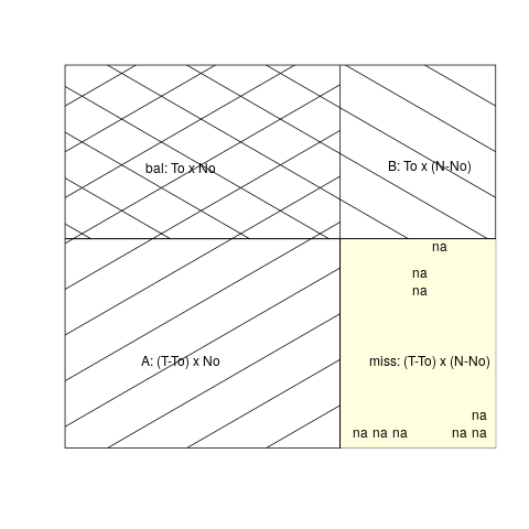
The key insight Bai and Ng (2021) is that $F$ and $\Lambda$ underlying the common component can be estimated from two blocks of completely observed data without reference to the missing data mechanism. In particular, the $T\times r$ matrix of factors can be consistently estimated from the tall block by PC. Since this only involves complete data estimation, PC can be replaced by PC-GLS or other consistent estimators, including maximum-likelihood. As discussed in Bai and Ng (2021), consistency of $\tilde{C}_{it}$ for $C_{it}$ requires that (i) the factor structure is strong in each block and as a whole, (ii) that the blocks are sufficiently similar, and (iii) strict stationarity with the same population moments in all blocks. Though the factor estimates are consistent without iteration, one re-estimation of $F$ and $\Lambda$ by applying PC to $\tilde{X}$ can accelerate the convergence rate of the estimated $C_{it}$ from $(\sqrt{N_{o}},\sqrt{T_{oi}})$ to $\sqrt{N_{ot}},\sqrt{T_{oi}})$ since $N_{o}\leq N_{ot}$. An appeal of the approach is that since $F$ and $\Lambda$ are estimated from completely observed data, a normal distribution theory for the imputed values can be obtained. Treating potential outcomes as missing values and assuming that the errors are serially uncorrelated, Bai and Ng (2021) obtain inferential results for the estimated average treatment effect.

We will apply tp to a mixed-frequency setting where of interest is $Y$, a high frequency series of length $T=\sum_{t=1}^{T_{o}}m_{t}$, $m_{t}$ being the number of sub-periods between $t$ and $t+1$. The observed values of $Y$ correspond to those of the low frequency series $y$ that is $T_{o}\times 1$. Though $Y$ is incompletely observed, it admits a factor representation

$$Y=F\Lambda_{Y}+e_{Y}.$$ (1)

Using $s_{t}=t+j/m_{t}$ for $j\in[1,m_{t}]$ to index the data in the higher frequency, we can also write $Y_{s_{t}}=\Lambda_{Y}^{\prime}F_{s_{t}}+e_{Y,s_{t}}.$ Without loss of generality, we will assume that data are released in the last sub-period between $t$ and $t+1$.

To impute the missing values in $Y$, tp exploits a $T\times N_{o}$ matrix $X_{o}$ assumed to have a factor structure $X_{o}=F\Lambda_{X_{o}}+e_{X_{o}}$. Hence in the tp setup, $X=(X_{o},Y)$. Complete data estimation of $F$ from $X_{o}$ (here, tall) yields $\tilde{F}$. The wide estimation reduces to regressing the low frequency series $y$ on the subvector of $\tilde{F}$ consisting of the last sub-period at every $t$. Assuming that $e_{Y}$ is unpredictable, tp will return

$$\tilde{Y}_{s_{t}}=\begin{cases}y_{t+1}\quad\quad\quad\quad&s_{t}=t+1\\ \tilde{\Lambda}_{Y}^{\prime}\tilde{F}_{s_{t}}&s_{t}=t+j/m_{t},\quad j\in[1,m_{t})\end{cases}.$$ (2)

According to tp, tall and wide suffice for imputation so long as $e_{Y}$ is serially uncorrelated.

3 Imputing Consumer Sentiment using the Static Procedures

We eventually want to interpolate weekly values of a monthly economic indicator. But as weekly data are not regularly spaced and weekly panels are typically smaller in size, we first test the procedures on regularly spaced monthly data which are abundantly available. Evaluating the adequacy of the interpolation methods is challenging when the values of interest were never released. In this section, we take advantage of the change in the release of one series to perform such an evaluation.

We consider a hypothetical exercise using the University of Michigan’s index of consumer sentiment (CS) as target. This series was available on a quarterly basis from 1960 to 1978 (specifically, in February, May, August, and November), but has been released on a monthly basis since 1978. The counterfactual exercise assumes that the CS series remained available on a quarter basis after 1978 and uses the different methods to impute the (2/3)$\times 504$ artificial missing monthly values. We first demean and standardize the CS series and then remove two observations each quarter in the early sample. The only series with missing values in the exercise is CS. The complete data matrix $X_{o}$ is a balanced monthly panel of 122 series taken from the December 2021 vintage of FRED-MD.

For joint estimation of the factors and missing values, we implement a Kalman smoother (KS) and the EM procedure of Stock and Watson (2002b). We also consider several estimators of $F$ for use in tp. To be clear about the exercise, different estimators of $F$ are used in tp, but the second (imputation) step is the same. These five estimators for $F$ are well known, we only summarize them in the Appendix. A detailed review is given in Barigozzi and Luciani (2019).

• the PC estimator $(\tilde{F},\tilde{\Lambda})=(\sqrt{T}U_{r},\sqrt{N}D_{r}V_{r})$ where $U_{r}$ and $V_{r}$ are the left and right singular vectors corresponding to the $r$ largest singular values collected in the diagonal entries of $D_{r}$. The PC estimates minimize $\text{tr}[(X-F\Lambda^{\prime})^{\prime}(X-F\Lambda)]$.

• Assuming joint normality of $X$ and $F$, an infeasible GLS estimator for $F$ which accounts for heteroskedasticity is:

  $$F^{GLS}_{s_{t}}=(\Lambda^{\prime}\Phi^{-1}\Lambda)^{-1}\Lambda^{\prime}\Phi^{-1}X_{s_{t}}.$$ (3)

  The MLE-h replaces $\Lambda$ and $\Phi$ with the maximum likelihood estimates analyzed in Bai and Li (2012).

• Breitung and Tenhofen (2011) use PC-GLS-har to account for both heteroskedasticity and serial correlation. We also consider a PC-GLS-h version that only controls for heteroskedasticity by updating the estimate of $F$ once using the PC estimates of $\Lambda$ and $\Phi$.

• An infeasible projections estimator that improves upon $\tilde{F}$ by using a VAR to model its dynamics is $F^{p}_{t}=\mathbf{U}_{t}^{\prime}\mathcal{F}^{p}$ where $\mathbf{U}_{t}^{\prime}=(\iota_{t}\otimes I_{r})$, $\iota_{t}$ is the $t$-th column of the identity matrix $I_{T}$,

  $$\mathcal{F}^{p}=E_{\Theta}(\mathcal{F}|\mathcal{X}] = \bigg{(}\Sigma_{\mathcal{F}}^{-1}+(I_{T}\otimes\Lambda^{\prime}\Phi^{-1}\Lambda)\bigg{)}^{-1}\bigg{(}(I_{T}\otimes\Lambda^{\prime}\Phi)\bigg{)}\mathcal{X},$$ (4)

  $\mathcal{F}=\text{vec}(F^{\prime})$, $\mathcal{X}=\text{vec}(X)$. The feasible estimator (PC-KS) uses the Kalman smoother to construct the required terms. We use the code implemented in Barigozzi and Luciani (2019).

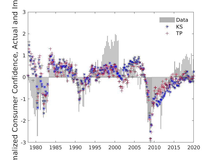
Figure 2: Monthly Consumer Confidence: Static

Figure 2 plots the normalized (demeaned and standardized) actual monthly consumer sentiment series (in grey) along with the series imputed by tp (red plus sign), and ks (blue asterisk). The series using mle-h, pc-gls-h, pc-gls-har, em, and pc-ks are not shown because they are similar to tp and ks. By construction, the imputed values coincide with the observed values once a quarter (hence not displayed as they coincide with the true values in gray). But notably, the imputed values bunched around zero which suggest that the missing values are not well predicted by the factor model. All methods significantly underestimate variability of the series since the imputed series have a standard deviation of only 0.75, much below that of the observed series, which is one. Re-estimation of the factors from the complete data matrix yields no noticeable improvements. Since tp and ks give similar imputed values, the problem appears not to be with joint or separate estimation of the factors and missing values. These results raise two questions. Why do different estimators of $F$ produce very similar results, and why are there episodes when estimates of missing values are bunched around zero?

3.1 A Calibrated Monte Carlo Exercise

We consider two calibrated experiments to understand why the choice of the estimator for the factors does not seem to matter. The first is calibrated to a balanced panel of $T=720$ observations for $N$= 122 series over the sample 1960:1-2019:12 in the 2021-12 vintage of FRED-MD, McCracken and Ng (2016). The parameters used in the simulations are based on PC estimation of $r=3$ factors. In this data, $\tilde{F}_{1}$ loads heavily on real activity variables and account for 0.147 of the total variation in the data, $\tilde{F}_{2}$ loads heavily on interest rates and account for .073, while $\tilde{F}_{3}$ loads heavily on prices and account for 0.070 of the total variation in the data. The implied idiosyncratic error variance $\tilde{\phi}_{i}$ range from 0.065 to 0.984, showing significant heteroskedasticity. The idiosyncratic errors are also serially correlated with $\rho_{i}$ ranging from -0.617 to 0.955. Estimation of a VAR(2) in the three factors finds the residuals to be mutually correlated. While $F_{2}$ has little serial correlation, $F_{1}$ is quite persistent.

The parameter estimates are used to simulate 1000 sets of data each with Nsim series of length $T=720$ by taking at each $t$, (i) $N$ independent normal draws of $e_{it}$, and (ii) $r$ normally distributed common shocks while holding the loadings fixed at the PC estimates. To ensure that the simulated data are representative of the original panel, the original panel is divided in three blocks of size (.4,.3,.3)$\times$ 122. Then (.4,.3, .3)$\times$ Nsim series are simulated from each of the three blocks. We vary Nsim from 10 to 122.

Table 1: DGP 1: $T=720,N=122,r=3$

	$M(F^{*},\hat{F})$
Nsim	10	20	30	40	50	75	122
PC	0.669	0.703	0.868	0.902	0.875	0.923	0.957
MLE-h	0.736	0.755	0.890	0.920	0.901	0.935	0.964
PC-GLS-h	0.774	0.785	0.890	0.921	0.901	0.935	0.964
PC-GLS-har	0.761	0.773	0.883	0.919	0.897	0.934	0.964
KS	0.759	0.789	0.895	0.922	0.909	0.936	0.964

Regression: $F^{*}_{j}=a+b_{1}\hat{F}_{1}+b_{2}\hat{F}_{2}+b_{3}\hat{F}_{3}$+ error Nsim 10 20 30 40 50 75 122 $R^{2}:j=$1 PC 0.736 0.841 0.897 0.936 0.922 0.956 0.971 MLE-h 0.793 0.872 0.919 0.947 0.935 0.962 0.976 PC-GLS-h 0.817 0.874 0.920 0.947 0.935 0.962 0.976 PC-GLS-har 0.790 0.856 0.916 0.946 0.933 0.961 0.976 KS 0.774 0.877 0.926 0.949 0.941 0.962 0.976 $R^{2}:j=$2 PC 0.628 0.614 0.868 0.877 0.861 0.907 0.954 MLE-h 0.713 0.686 0.886 0.903 0.896 0.924 0.962 PC-GLS-h 0.769 0.741 0.885 0.905 0.897 0.924 0.962 PC-GLS-har 0.769 0.740 0.879 0.901 0.893 0.923 0.962 KS 0.770 0.743 0.888 0.905 0.902 0.924 0.962 $R^{2}:j=$3 PC 0.642 0.655 0.837 0.891 0.842 0.905 0.946 MLE-h 0.700 0.706 0.864 0.910 0.870 0.920 0.954 PC-GLS-h 0.736 0.738 0.864 0.911 0.870 0.920 0.954 PC-GLS-har 0.722 0.722 0.853 0.909 0.864 0.919 0.954 KS 0.729 0.745 0.871 0.912 0.883 0.921 0.954

Notes: The top panel reports

$$M(F^{*},\hat{F})=\frac{\text{trace}(F^{*^{\prime}}\hat{F}(\hat{F}^{\prime}\hat{F})^{-1}\hat{F}^{\prime}F^{*})}{\text{trace}(F^{*^{\prime}}F^{*})},$$

which measures the multivariate correlation between $F^{*}$ and their estimates $\hat{F}$. The bottom panel reports the $R^{2}_{j}$ from each $F_{j}^{*}$ regressed on $\hat{F}_{1},\ldots,\hat{F}_{r}$. $F_{j}^{*}$ is estimated according to procedures listed in section 3: (i) PC; (ii) MLE-h; (iii) GLS-h; (iv) GLS-har; (v) KS.

Two sets of results are given in Table 3.1. The top panel reports

$$M(F^{*},\hat{F})=\frac{\text{trace}(F^{*^{\prime}}\hat{F}(\hat{F}^{\prime}\hat{F})^{-1}\hat{F}^{\prime}F^{*})}{\text{trace}(F^{*^{\prime}}F^{*})},$$

which measures the multivariate correlation between $F^{*}$ and their estimates $\hat{F}$. The PC estimates have noticeably larger errors when Nsim is smaller than 50. However, even when Nsim is not small, there is little to gain in modeling dynamics of $F$ or of $e$ over controlling for heteroskedasticity.

Next, each $F_{j}^{*}$ is regressed on $\hat{F}_{1},\ldots,\hat{F}_{r}$ and the regression $R^{2}_{j}$ is used as indicator of how well information in $F^{*}_{j}$ is captured by $\tilde{F}$. These $R^{2}_{j}$s are reported in the bottom panel of Table 3.1. Three results are of note. First, the improvements over PC are larger for estimates of $F_{2}$ and $F_{3}$ than for $F_{1}$. Second, while the improvements in $R^{2}$ are noticeable when Nsim=10, they diminish rapidly when Nsim exceeds 30. Third, and reinforcing the observation made above, the gains of modeling the dynamics of $F$ over a GLS correction for heteroskedasticity are quite small.

We also consider a second experiment that restricts the panel to the first $N=50$ variables in the panel which are all on real activity variables, over a shorter sample that starts in 1978 with $T=420$ observations. This time, the parameters used to simulate data are estimated by maximum likelihood. The first factor in this data is also a real activity factor and all methods estimate it very well. As seen in Table 3.1, the maximum likelihood estimates of $F_{1}$ are only slightly better than the PC estimates when Nsim=10. The efficiency gains in estimating $F_{2}$ are more noticeable. The gains from using the Kalman smoother are large at Nsim=10 but become much smaller when Nsim=30.

Table 2: DGP2: $T=420,N=50$, $r=2$

Regression: $F^{*}_{j}=a+b_{1}\hat{F}_{1}+b_{2}\hat{F}_{2}+b_{3}\hat{F}_{3}$+ error

Notes: The top panel reports

$$M(F^{*},\hat{F})=\frac{\text{trace}(F^{*^{\prime}}\hat{F}(\hat{F}^{\prime}\hat{F})^{-1}\hat{F}^{\prime}F^{*})}{\text{trace}(F^{*^{\prime}}F^{*})},$$

which measures the multivariate correlation between $F^{*}$ and their estimates $\hat{F}$. The bottom panel reports the $R^{2}_{j}$ from each $F_{j}^{*}$ regressed on $\hat{F}_{1},\ldots,\hat{F}_{r}$. $F_{j}^{*}$ is estimated according to procedures listed in section 3: (i) PC; (ii) MLE-h; (iii) GLS-h; (iv) GLS-har; (v) MLE-ks.

To understand why the alternatives to PC perform so similarly, we need to understand the properties of projections estimators. Bai and Li (2012) consider a projections estimator that only controls for heteroskedasticity:

$$F_{t}^{p}=E_{\Theta}[F_{t}|X_{1},\ldots,X_{T}]=\bigg{(}\Sigma^{-1}_{F}+\Lambda^{\prime}\Phi^{-1}\Lambda\bigg{)}^{-1}\Lambda^{\prime}\Phi^{-1}X_{t}.$$ (5)

A Woodbury inversion of $\mathcal{G}=(\Sigma_{F}^{-1}+\Lambda^{\prime}\Phi^{-1}\Lambda)^{-1}$ yields:

$$F_{t}^{p} = (\Lambda^{\prime}\Phi^{-1}\Lambda)^{-1}\Lambda^{\prime}\Phi^{-1}X_{t}-\mathcal{G}\Sigma_{F}^{-1}(\Lambda^{\prime}\Phi^{-1}\Lambda)^{-1}\Phi^{-1}X_{t}.$$

But the first term is simply the infeasible GLS estimator and the second term converges to zero in mean square under the assumptions of a strong factor model. This leads to the result in Doz et al. (2012) and Bai and Li (2016) that

$$F^{p}_{t}=F_{t}^{GLS}+O(N^{-1/2})$$

which is to say that the projections estimator is asymptotically equivalent to the GLS estimator that only controls for heteroskedasticity.

Now consider PC-KS that also accounts for the dynamics of $F$. A Woodbury inversion of $\mathcal{G}=\Sigma_{\mathcal{F}}^{-1}+(I_{T}\otimes\Lambda^{\prime}\Phi^{-1}\Lambda)$ yields

$$F^{p}_{t} = F^{GLS}_{t}-\mathbf{U}_{t}^{\prime}\mathcal{G}\Sigma^{-1}_{\mathcal{F}}\mathcal{F}-\mathbf{U}_{t}^{\prime}\mathcal{G}\Sigma_{F}^{-1}(I_{T}\otimes(\Lambda^{\prime}\Phi^{-1}\Lambda)^{-1})\Lambda^{\prime}\Phi^{-1}\mathcal{E}$$

where $\mathcal{E}=\text{vec}(e)$ is $NT\times 1$. Consistency of the (infeasible) projections estimator for $F_{t}$ follows because $F_{t}^{GLS}\smash{\mathop{\longrightarrow}\limits^{p}}F_{t}$ and the second term vanishes at rate $\sqrt{N}$. The feasible PC-KS estimator is also consistent for $F$. While consistency of the estimator is recognized, less appreciated is that it is asymptotically equivalent to the GLS estimator that only controls for heteroskedasticity. Indeed, Bai and Li (2016) show that $\hat{F}^{PC-KS}_{t}-\hat{F}^{GLS}_{t}=O_{p}(N^{-1/2})+O_{p}(T^{1/2}N^{-2})$ if $T/N^{3}\rightarrow 0$, where $\hat{F}_{t}^{KS}$ and $\hat{F}_{t}^{GLS}$ are the QMLE estimates of $\Lambda$, $\Phi$, $\Sigma_{\mathcal{F}}$.

An overlooked feature of projections estimators is that they are shrinkage estimators that shrink towards $F_{s_{t}}^{GLS}$. The degree of shrinkage depends on the relative importance of each factor and will be larger for factors with smaller variances. As seen from Table 3.1, the less important factors stand to gain more from shrinkage. Furthermore, to the extent that $F_{s_{t}}^{GLS}$ is unbiased, the shrinkage estimators will be biased, but the smaller variance may result in a more favorable mean-squared error. Under the strong factor assumption, $\Lambda^{\prime}\Phi^{-1}\Lambda$ is $O_{p}(N)$ while $\Sigma^{-1}_{F}$ does not increase with $N$. Hence, the shrinkage factor will vanish as $N$ increases. Our calibrated Monte Carlo simulation results are consistent with theory. Controlling for heteroskedasticity in the idiosyncratic errors generates the largest improvements over the PC estimates of $F$.

In summary, whether the idiosyncratic errors are serially correlated or heteroskedastic, estimators more efficient than PC are available. The above Monte Carlo experiments confirm that gains do appear in finite samples. But in the empirical exercise when $N$ is quite large, all consistent estimators of $F$ produce similar imputed values. Though these will be unbiased provided $\mathbb{E}[e_{t}]=0$, they are unfortunately bunched around the normalized unconditional mean of zero. But as Phillips (1979) noted, prediction is made given the final value of the endogenous variable in practice. In the next section, we will argue that the bunching arises when the realized $e_{T}$ is not zero. We then suggest different ways to incorporate the information into the imputation.

4 Dynamic Imputation

This section considers three ways to account for residual serial correlation in imputation given related covariates. The first is the seminal work of Chow and Lin (1971). The second is an iterative algorithm that estimates a factor-augmented autoregressive distributed lag model from incomplete data. The third is joint modelling of the latent factors and missing values while accounting for residual serial correlation in a fully specified state space system. The first and third methods produce smoothed estimates that use information beyond the period that the missing value occurs. The third method is fully specified and can be more efficient but is computationally costly. Thus, each method has some appeal.

4.1 The Chow-Lin Procedure

Chow and Lin (1971) provide a methodology for best linear unbiased extrapolation and interpolation of a time series using a small set of related variables. The analysis is built on the classic result of Goldberger (1962) that analyzes the case when complete data are available for estimation of a linear prediction model $Y=Z\beta+u$ in which the errors are non-spherical. The best linear unbiased prediction (BLUP) of some $Y_{T+\ell}$ when predictors $Z_{T+\ell}$ are available takes the form $\hat{Y}_{T+\ell}=Z_{T+\ell}^{\prime}\hat{\beta}+\mathbb{E}[u_{T+\ell}u^{\prime}]^{\prime}V^{-1}\hat{u}$, where $\hat{u}=Y-Z\hat{\beta}$ is the vector of in-sample residuals, and $\hat{\beta}$ is the GLS estimator. In the AR(1) case when $u_{t}=\rho u_{t-1}+\epsilon_{t}$, the BLUP simplifies to $\hat{Y}_{T+\ell}=Z_{T}^{\prime}\hat{\beta}+\rho^{\ell}u_{T}$. The equivalent representation $\hat{Y}_{T+1}=Z_{T}^{\prime}\hat{\beta}+\rho(y_{T}-Z_{T}\hat{\beta})$ for $\ell=1$ was suggested in Cochrane and Orcutt (1949) as a way to improve prediction efficiency when the errors are correlated. Note that though the omitted term $\rho^{\ell}u_{T}$ does not create unconditional bias so long as $\mathbb{E}[u_{T}]=0$, omitting the second term can induce bias if the $u_{T}$ in the data is non-zero.

The Chow-Lin analysis is more complicated because data of different frequencies are involved and a matrix $C$ is needed to map the data from one frequency to another. The target is a vector of non-sampled values, say, $q_{*}$. For interpolating stock variables, each row of $C$ would have a single non-zero entry to indicate which subperiod is observed, while for flow data, each row of $C$ would have $m_{t}$ non-zero entries to pick the sub-periods that are to be aggregated. The Goldberger (1962) analysis is a special case when $C$ is an identity matrix. To make our point clear, we only consider stock variables which is also notationally simpler.

We will subscript variables by $H$ or $L$ when we are referring to the Chow-Lin procedure. Let $Z_{H}$ be a $T_{H}\times K$ matrix of observed high frequency predictors for $Y_{H}$ modeled as

$$Y_{H}=Z_{H}B+u_{H},\quad\quad u^{H}\sim(0,V_{H}).$$

Multiplying both sides by the $T_{L}\times T_{H}$ predetermined matrix $C$ gives the bridge equation

$$Y_{L}=Z_{L}B+u_{L},\quad\quad u_{L}\sim(0,V_{L})$$ (6)

where $V_{L}=CV_{H}C^{\prime}$, $CY_{H}=Y_{L}$, $CZ_{H}=Z_{L}$ and $u_{L}=Cu_{H}$. The goal is to obtain linear unbiased imputation of $q_{*}$ when $u_{*}=u_{H}$. To do so, Chow and Lin (1971) consider linear predictors of the form by $\hat{q}_{*}=AY_{L}=A(Z_{L}+u_{L})$ where $A$ is $T_{*}\times T_{L}$, and minimize trace(cov$(\hat{q}_{*}q_{*}))$ with respect to $A$ subject to the linear-unbiased constraint that $AZ_{L}-Z_{*}=0$. Though $B$ is identifiable from the low frequency bridge equation, terms do not simplify as in Goldberger (1962) because $C$ is no longer an identity matrix. Nonetheless, the (infeasible) BLUP of $q_{*}$ has a familiar form:

$$\mathbb{E}[q_{*}|Z_{H},Y_{L}]=Z_{H*}^{\prime}\hat{\beta}_{GLS}+\mathbb{E}[u_{*}u_{L}^{\prime}]^{\prime}V_{L}^{-1}\hat{u}_{L}$$ (7)

where $\hat{\beta}_{GLS}$ estimates $\beta=(Z_{L}^{\prime}V_{L}^{-1}Z_{L})^{-1}Z_{L}^{\prime}V_{L}^{-1}Y_{L}$. As in Goldberger (1962), the solution has two components. The first combines the high frequency information $Z_{H}$ as predictors with GLS estimates of $\beta$ as weights to form the conditional mean. When $u_{H}$ is serially correlated, the second distributes the low frequency error $\hat{u}_{L}$ to the sub-periods between $t$ and $t+1$ under an assumed error structure. Chow and Lin (1971) assume an AR(1) model for $u_{H}$ while Fernandez (1981); Litterman (1983) considers higher order persistence. Though the $V_{H}$ matrices differ, the idea is the same.

In spite of the popularity of the Chow-Lin procedure, there is little discussion of how $\hat{u}_{L}$ is actually distributed in the remaining $m_{t}-1$ sub-periods. Note that $q^{*}$ is not sampled and thus unobserved after the fact, which complicates evaluation of procedures. With the help of some symbolic math calculations, we find that for AR(1) errors parameterized by $\rho$, the procedure produces

$$\hat{Y}_{H,s_{t}} = \hat{\beta}_{GLS}^{\prime}Z_{H,s_{t}}+\hat{\theta}_{1,s_{t}}\hat{u}^{L}_{t}+\hat{\theta}_{2,s_{t+1}}\hat{u}^{L}_{t+1}$$

$$= \hat{\beta}_{GLS}^{\prime}Z_{H,s_{t}}+\hat{\theta}_{1,s_{t}}\bigg{(}Y_{L,t}-\hat{\beta}_{GLS}^{\prime}Z_{L,t}\bigg{)}+\hat{\theta}_{2,s_{t+1}}\bigg{(}Y_{L,t+1}-\hat{\beta}_{GLS}^{\prime}Z_{L,t+1}\bigg{)}$$

where the weights $\hat{\theta}_{1,s_{t}}$ and $\hat{\theta}_{2,s_{t+1}}$ depend on $\rho$ and are different at the endpoints from the interior of the sample. The interesting feature is that in the $m_{t}-1$ sub-periods when $Y_{H,s_{t}}$ is missing, $\tilde{Y}_{H,s_{t}}$ will only depend on $\hat{u}_{L,t}$ and $\hat{u}_{L,t+1}$ but not values of $\hat{u}_{L}$ before $t$ or after $t+1$. This is intuitive in retrospect because $s_{t}\in(t,t+1]$. By using information in $t+1$, the Chow-Lin procedure obtains a smoothed estimate of the serially correlated noise. The non-zero weights also imply that the imputed series will be smoother than when $\rho$ is assumed to be zero.

There are variations to the Chow-Lin procedure, many motivated by the unsynchronized release of macroeconomic data towards the end of the sample. The so-called ragged-edge problem noted in Wallis (1986) has generated much interests in extrapolating the target variable using data that are incompletely released, also known as nowcasting. The MIDAS (mixed-data sampling) approach of Ghysels (2006) replaces $Z_{H}B$ by a distributed lag of $Z_{H}$ with parameters $\delta_{H}$ to be jointly estimated with $B$ by constrained non-linear least squares, but without imposing the unbiased constraint. Schumacher (2016) suggests that the difference between MIDAS and Chow-Lin type procedures is akin to direct versus iterative forecasts. The UMIDAS of Foroni and Marcellino (2014) estimates $\delta_{H}$ freely. tp is most closely related to UMIDAS with $Z_{H}$ replaced by $\tilde{F}$.

4.2 TP*

The Chow and Lin (1971) procedure models persistence in the residuals. Santos Silva and Cardoso (2001) rewrite the model in terms of an infinite order distributed lag in $Z_{H}$ that is eventually approximated by a finite number of lags. Ghysels et al. (2005) caution in the context of MIDAS that this way of introducing autoregressive dynamics in mixed frequency estimation can generate spurious periodic responses. To circumvent this problem, Clements and Galvao (2008) add common autoregressive dynamics to both $Y_{L}$ and the predictors in the bridge equation. In the spirit of Chow and Lin (1971), lead and lagged information pertain to those of $Y_{L}$ through the bridge equation.

Why not directly use lags of $Y_{H}$? The challenge is that $Y_{H}$ is incompletely observed. In spite of early contributions from Sargan and Drettakis (1974); Dunsmuir and Robinson (1981); Palm and Nijman (1984), the literature on estimating dynamic models with missing data remains quite small. Palm and Nijman (1984) consider identification issues in estimation of ARMA models with missing data. In the missing data literature developed mostly for i.i.d. data with focus on parameter estimation and not the missing values themselves, the generic procedure is to use sweep operations to first predict the missing values one variable at a time, irrespective of whether the variable is a covariate or dependent variable. The output is then used to adjust the sufficient statistics for bias due to missing values. As illustrated in Little and Rubin (2019, Ch. 11) for the AR(1) model where $y_{1},y_{3},\ldots,y_{T-1}$ are observed but not $y_{2},y_{4},\ldots,y_{T}$, the adjustments require an implicit regression of $y_{t}$ on $y_{t-1},y_{t+1}$. Hence like the Chow-Lin procedure, forward information up to $t+1$ is incorporated without directly using the Kalman filter. However, the bias adjustments are model specific and the sweep operations can be cumbersome to implement.

We consider an approach that is easy to implement but is less efficient because it uses only lagged information. Suppose that $u_{H,s_{t}}=\rho u_{H,s_{t}-1/m_{t}}+\epsilon^{0}_{H,s_{t}}$. Quasi differencing at $\rho$ gives

$$Y_{H,s_{t}}=Z_{H,s_{t}}^{\prime}\beta+\rho(Y_{H,s_{t}-1/m_{t}}-\beta^{\prime}Z_{H,s_{t}-1/m_{t}})+\epsilon^{0}_{H,s_{t}}.$$

When $\rho\neq 0$, the lagged error of the static model, though mean zero, contains information to improve the prediction. The unrestricted form of the above equation is the equation in Durbin (1970)

$$Y_{H,s_{t}}=\rho Y_{H,s_{t}-1/m_{t}}+\beta^{\prime}Z_{H,s_{t}}+\gamma^{\prime}Z_{H,s_{t}-1/m_{t}}+\epsilon_{s_{t}}.$$

The problem is transformed from a bridge regression in completely observed low frequency data with a serially correlated error, to a regression in high frequency data with a serially uncorrelated error, but that the dependent and lagged dependent variable are incompletely observed.

A naive approach is to use deterministic rules to interpolate the missing values between $t$ and $t+1$, such as replacing all missing $y_{s_{t}}$ for $s_{t}\in(t,t+1]$ with the most recently observed value, $y_{t}$. This can conveniently accommodate irregular missing patterns but would not incorporate the available high frequency information between $t$ and $t+1$. We suggest to improve upon the naive approach by iteratively updating the imputed series. Starting at $k=0$, we estimate $\rho^{(k)},\beta^{(k)}$ and $\gamma^{(k)}$ from

$$Y^{(k)}_{H,s_{t}}=\rho Y^{(k)}_{H,s_{t}-1/m_{t}}+\beta^{\prime}Z_{H}+\gamma^{\prime}Z_{H,s_{t}-1/m_{t}}+\epsilon_{s_{t}}.$$

Then for those $s_{t}$ for which $Y_{H,s_{t}}$ are not observed, we set $Y^{(k+1)}$ to $\hat{Y}_{H,s_{t}}=\hat{\rho}^{(k)}Y^{(k)}_{H,s-1}+Z_{H,s-1}^{\prime}\hat{\beta}^{(k)}+Z_{H,s-1}^{\prime}\hat{\gamma}^{(k)}$ and update $k$ to $k+1$. Iteration stops when $|Y^{(k+1)}-Y^{k}|$ is less than some tolerance. Iterative estimation of missing values seems to date back to Healy and Westmacott (1956) but is mainly used in i.i.d. settings. In the two pen-and-pencil cases considered, we can show that the converged estimates are the true values and that a sign restriction on $\rho$ is needed to ensure a unique solution, consistent with the result in Palm and Nijman (1984).

To help understand the difference between Chow-Lin and the iterative procedure, consider a simple example with $m_{t}=m=3$. The iterative procedure would impute $Y_{H,1+2/3}$ as

$$\hat{Y}_{H,t+2/3} = \hat{\alpha}\hat{Y}_{H,t+1/3}+\hat{\gamma}_{1}^{\prime}Z_{H,t+2/3}+\hat{\gamma}_{2}^{\prime}Z_{H,t+1/3}$$

$$= \hat{\alpha}\bigg{(}\hat{\alpha}Y_{H,t}+\hat{\gamma}_{1}^{\prime}Z_{H,t+1/3}+\hat{\gamma}_{2}^{\prime}Z_{H,t}\bigg{)}+\hat{\gamma}_{1}^{\prime}Z_{H,t+2/3}+\hat{\gamma}_{2}^{\prime}Z_{H,t+1/3}$$

$$= \hat{\delta}_{Y}^{\prime}Y_{H,t}+\hat{\delta}_{Z,0}Z_{H,t}+\hat{\delta}_{Z,1}^{\prime}Z_{H,t+1/3}+\hat{\delta}_{Z,2}^{\prime}Z_{H,t+2/3},$$

which is a weighted sum of $Y_{H,t}$, $Z_{H,t},Z_{H,t+2/3},Z_{H,1+t/3}$, and the $\delta$ parameters are estimated by OLS. Using the fact that $Y_{L,t}=Y_{H,t}$, $Z_{L,t}=Z_{H,t}$ and $Z_{L,t+1}=Z_{H,t+1}$, the Chow-Lin procedure returns

$$\hat{Y}_{H,t+2/3}=\hat{\beta}_{GLS}^{\prime}Z_{H,t+2/3}+\hat{\theta}_{1,t}(Y_{H,t}-\hat{\beta}_{GLS}^{\prime}Z_{H,t})+\hat{\theta}_{2,t}(Y_{L,t+1}-\hat{\beta}_{GLS}^{\prime}Z_{L,t+1}),$$

which is a weighted sum of $Y_{H,t},Z_{H,t},Z_{H,t+2/3}$ and $Y_{H,t+1},Z_{H,t+1}$, and the parameters are estimated by GLS. Notably, the iterative procedure does not include $t+1$ information, but it incorporates $Z_{H,t+1/3}$ not used in Chow-Lin.

With this background, we can now modify tp to tp* so that wide step is iterative estimation of an autoregressive distributed lag regression. Starting at $k=0$ with $Y_{s_{t}}^{(0)}=\tilde{Y}_{s_{t}}$ , estimate

$$Y^{(k)}_{s_{t}}=\beta_{0}+\rho Y^{(k)}_{s_{t}-1/m_{t}}+\Gamma_{Y}(L)^{\prime}\tilde{F}_{s_{t}-1/m_{t}}+w_{Y,s_{t}}.$$ (8)

The fit is then used to update $Y^{(k+1)}_{s_{t}}$ if $Y_{s_{t}}$ is missing at $s_{t}$. Separating the task of estimating $F$ from imputation provides a way to control for serial correlation in $e_{Y,s_{t}}$ without changing estimation of $F$. Note that while static tp does not require iteration, tp* does require iteration to ensure that the $Y$ and lagged values used in the regression are internally consistent. It can be used with any estimator of $F$ in the tall step.

4.3 A Modified Kalman Filter

tp* is what Banbura et al. (2013) refer to as partial approach that do not specify a joint model for the variable of interest. A systems approach is more efficient but can be computationally costly. With this approach, we model the data $X_{s_{t}}=(X_{o,s_{t}}^{\prime},Y_{s_{t}})^{\prime}$ as being driven by latent factors $\mathcal{F}_{s_{t}}$ and serially correlated idiosyncratic errors $\tilde{\epsilon}_{is_{t}+1/mt}$

Observation Equation: $$X_{s_{t}} =\Lambda\mathcal{F}_{s_{t}}+\epsilon_{s_{t}}$$

$$\epsilon_{is_{t}} =\tilde{\epsilon}_{is_{t}}+\xi_{is_{t}} \xi_{is_{t}}\sim N\left(0,\sigma^{2}_{\xi i}\right)$$

$$\tilde{\epsilon}_{is_{t}+1/m_{t}} =\rho_{i}\tilde{\epsilon}_{is_{t}}+e_{is_{t}+1/m_{t}} e_{is_{t}}\sim N\left(0,\sigma^{2}_{ei}\right)$$

Transition Equation: $$\mathcal{F}_{s_{t}+1/m_{t}} =\mathcal{A}\mathcal{F}_{s_{t}}+\eta_{s_{t}} \eta_{s_{t}}\sim N\left(0,\Sigma_{\eta}\right)$$

where $\epsilon_{s_{t}}=\left(\epsilon_{1s_{t}},\epsilon_{2s_{t}},\epsilon_{N_{0}s_{t}}\epsilon_{Ys_{t}}\right)^{\prime}$, $e_{s_{t}}$, $\xi_{s_{t}}$, and $\tilde{\epsilon}_{s_{t}}$ are similiarly defined. The issue is that the standard Kalman filter and smoothing equations such as in Durbin and Koopman (2002) cannot be applied because some equations are not standard observation and transition form. Jungbacker et al. (2011) provides a method to account for residual serial correlation in a state-space setup but requires that we observe two sequential values of the target variable. The weekly data that we will subsequently consider are irregularly spaced.

In order to model the residual serial correlation in the presence of missing errors in a tractable manner, we combine two existing techniques of compressing the extra processes: quasi-differencing (Method A), and expanding the state space (Method B). Quasi differencing is computationally tractable for large datasets, but is not appropriate for series with missing data. Expanding the state space is theoretically feasible for datasets with missing data, but empirically impractical because of the computation cost - the number of latent states increases with the number of variables in the dataset. Our proposed approach is to quasi difference series for which data are completely observed, and only add a series-specific predictable component to the state vector for our target variable which has missing values in the high frequency. We briefly review the two methods that are combined before presenting the proposed state space setup. There are $r$ factors in the general case, $\mathcal{F}_{t}=\left(\mathcal{F}_{1t},\mathcal{F}_{2t},\dots,\mathcal{F}_{rt}\right)^{\prime}$. We use a two factor case as an example for Method B and our proposed procedure.

Method A: Accounting for Serial Correlation with Quasi Differencing

This method follows Watson and Engle (1983); Reis and Watson (2010). Define $\rho=\text{diag}\left(\rho_{1},\dots,\rho_{N_{0}},\rho_{Y}\right)$. Quasi differencing both the left and right hand side of the observation equation $X_{s_{t}}=\Lambda\mathcal{F}_{s_{t}}+\epsilon_{s_{t}}$ gives

$$\left(\mathbb{I}-\rho L\right)X_{s_{t}} =\left(\mathbb{I}-\rho L\right)\left(\Lambda\mathcal{F}_{s_{t}}+\epsilon_{s_{t}}\right)$$

$$X_{s_{t}}-\rho X_{s_{t}-1/m_{t}} =\Lambda\mathcal{F}_{s_{t}}-\rho\Lambda\mathcal{F}_{s_{t}-1/m_{t}}+\epsilon_{s_{t}}-\rho\epsilon_{s_{t}-1/m_{t}}$$

Note that $\epsilon_{s_{t}}-\rho\epsilon_{s_{t}-1/m_{t}}=e_{s_{t}}$. Rearranging terms yields

$$X_{s_{t}} =\underset{c_{s_{t}}}{\underbrace{\rho X_{s_{t}-1/m_{t}}}}+\underset{\Lambda^{A}}{\underbrace{\left(\Lambda,-\rho\Lambda\right)}}\underset{\mathcal{F}_{s_{t}}^{A}}{\underbrace{\begin{pmatrix}\mathcal{F}_{s_{t}}\\ \mathcal{F}_{s_{t}-1/m_{t}}\end{pmatrix}}}+e_{s_{t}}$$

In state space formulation, the observation equation can be replaced with

$$X_{s_{t}} =c_{s_{t}}+\Lambda^{A}\mathcal{F}_{s_{t}}^{A}+e_{s_{t}}$$

Where $e_{s_{t}}\sim N\left(0,\text{diag}\left(\sigma^{2}_{e1},\dots\sigma^{2}_{eN_{0}},\sigma^{2}_{eY}\right)\right)$, thus pre-removing serial correlation. The term $c_{s_{t}}$ is known at time $s_{t}$ and can be easily accounted for in the updating equations.

Method B: Accounting for Serial Correlation by Expanding the State Space

This method follows Banbura and Modugno (2014). Consider a two factor model, $\mathcal{F}_{s_{t}}=\left(\mathcal{F}_{1s_{t}},\mathcal{F}_{2s_{t}}\right)^{\prime}$. The transition equation for the factors can be written as

$$\begin{pmatrix}\mathcal{F}_{1s_{t}+1/m_{t}}\\ \mathcal{F}_{2s_{t}+1/m_{t}}\end{pmatrix}=\begin{pmatrix}\mathcal{A}_{11}&\mathcal{A}_{12}\\ \mathcal{A}_{13}&\mathcal{A}_{22}\end{pmatrix}\begin{pmatrix}\mathcal{F}_{1s_{t}}\\ \mathcal{F}_{2s_{t}}\end{pmatrix}+\begin{pmatrix}\eta_{1s_{t}+1/m_{t}}\\ \eta_{2s_{t}+1/m_{t}}\end{pmatrix}$$

The autocorrelated part of the idiosyncratic errors $\tilde{\epsilon}_{is_{t}}$ can be added to the state space for all $N$ variables

$$\underset{\mathcal{F}_{s_{t}+1/m_{t}}^{B}}{\underbrace{\begin{pmatrix}\mathcal{F}_{1s_{t}+1/m_{t}}\\ \mathcal{F}_{2s_{t}+1/m_{t}}\\ \tilde{\epsilon}_{1s_{t}+1/m_{t}}\\ \tilde{\epsilon}_{2s_{t}+1/m_{t}}\\ \vdots\\ \tilde{\epsilon}_{Ys_{t}+1/m_{t}}\end{pmatrix}}}=\underset{\mathcal{A}^{B}}{\underbrace{\begin{pmatrix}\mathcal{A}_{11}&\mathcal{A}_{12}&0&0&\dots&0\\ \mathcal{A}_{21}&\mathcal{A}_{22}&0&0&\dots&0\\ 0&0&\rho_{1}&0&\dots&0\\ 0&0&0&\rho_{2}&\dots&0\\ 0&0&0&0&\ddots&0\\ 0&0&0&0&\dots&\rho_{Y}\end{pmatrix}}}\underset{\mathcal{F}_{s_{t}}^{B}}{\underbrace{\begin{pmatrix}\mathcal{F}_{1s_{t}}\\ \mathcal{F}_{2s_{t}}\\ \tilde{\epsilon}_{1s_{t}}\\ \tilde{\epsilon}_{2s_{t}}\\ \vdots\\ \tilde{\epsilon}_{Ys_{t}}\end{pmatrix}}}+\underset{\eta_{s_{t}}^{B}}{\underbrace{\begin{pmatrix}\eta_{1s_{t}+1/m_{t}}\\ \eta_{2s_{t}+1/m_{t}}\\ e_{1s_{t}+1/m_{t}}\\ e_{2s_{t}+1/m_{t}}\\ \vdots\\ e_{Ys_{t}+1/m_{t}}\end{pmatrix}}}$$

Define:

$$\Lambda^{B}\equiv\begin{pmatrix}\Lambda&\mathbf{0}_{N\times N}\\ \mathbf{0}_{N\times N}&\mathbb{I}_{N}\end{pmatrix}$$

Thus the observation equation can be rewritten in a form of a serially uncorrelated idiosyncratic error

$$X_{s_{t}} =\Lambda^{B}\mathcal{F}^{B}_{s_{t}}+\xi_{s_{t}}$$

where $\xi_{s_{t}}\sim N\left(0,\text{diag}\left(\sigma^{2}_{\xi 1},\dots,\sigma^{2}_{\xi N_{0}},\sigma^{2}_{\xi Y}\right)\right)$.

Proposed KS*

While quasi differencing the data is preferred as it does not increase the estimated state space, it can be applied only if we observe two sequential values of the target variable. As missing values can be irregularly spaced as in the case of weekly data, we write the state space system using a combination of the two methodologies described above: completely observed variables are quasi differenced, and the autocorrelation of the serially correlated error of the target series is included as an additional state. Consider again a two factor model. We can rewrite the transition equation as follows

$$\begin{pmatrix}\mathcal{F}_{1s_{t}+1/m_{t}}\\ \mathcal{F}_{2s_{t}+1/m_{t}}\\ \tilde{\epsilon}_{Ys_{t}+1/m_{t}}\end{pmatrix}=\underset{\mathcal{A}^{*}}{\underbrace{\begin{pmatrix}\mathcal{A}_{11}&\mathcal{A}_{12}&0\\ \mathcal{A}_{21}&\mathcal{A}_{22}&0\\ 0&0&\rho_{Y}\end{pmatrix}}}\begin{pmatrix}\mathcal{F}_{1s_{t}}\\ \mathcal{F}_{2s_{t}}\\ \tilde{\epsilon}_{Ys_{t}}\end{pmatrix}+\underset{\eta_{s_{t}}^{*}}{\underbrace{\begin{pmatrix}\eta_{1s_{t}+1/m_{t}}\\ \eta_{2s_{t}+1/m_{t}}\\ e_{Ys_{t}+1/m_{t}}\end{pmatrix}}}$$

We can then take into account serial correlation of the completely observed series using quasi differencing in the observation equation. In this framework, however, define $\rho^{*}=\text{diag}\left(\rho_{1},\dots,\rho_{N_{0}},0\right)$. The observation equation is then

$$X_{s_{t}} =\underset{c_{s_{t}}}{\underbrace{\rho^{*}X_{s_{t}-1/m_{t}}}}+\underset{\Lambda^{*}}{\underbrace{\left(\Lambda,-\rho^{*}\Lambda,\begin{pmatrix}\mathbf{0}_{N_{0}\times 1}\\ 1\end{pmatrix}\right)}}\begin{pmatrix}\mathcal{F}_{s_{t}}\\ \mathcal{F}_{s_{t}-1/m_{t}}\\ \tilde{\epsilon}_{Ys_{t}}\end{pmatrix}+\begin{pmatrix}e_{1s_{t}}\\ \vdots\\ e_{N_{0}s_{t}}\\ \xi_{Ys_{t}}\end{pmatrix}$$

The state space comprises of the original latent factors, the lags of these factors, and one additional state for the predictable residual component. This combined approach remains computationally tractable for large $N$. In implementation, we modified the code from Barigozzi and Luciani (2019)..

4.4 Re-examining the CS Series

We now return to the example considered earlier where $Y$ is the incompletely observed consumer sentiment series, and show that treatment of the dynamics of the idiosyncratic error is more important than the estimation procedufre for the common factors. The top panel of Figure 3 compares the static tp estimate with the dynamic estimate tp*, where the latter includes one lag of both $F$ and $Y$.

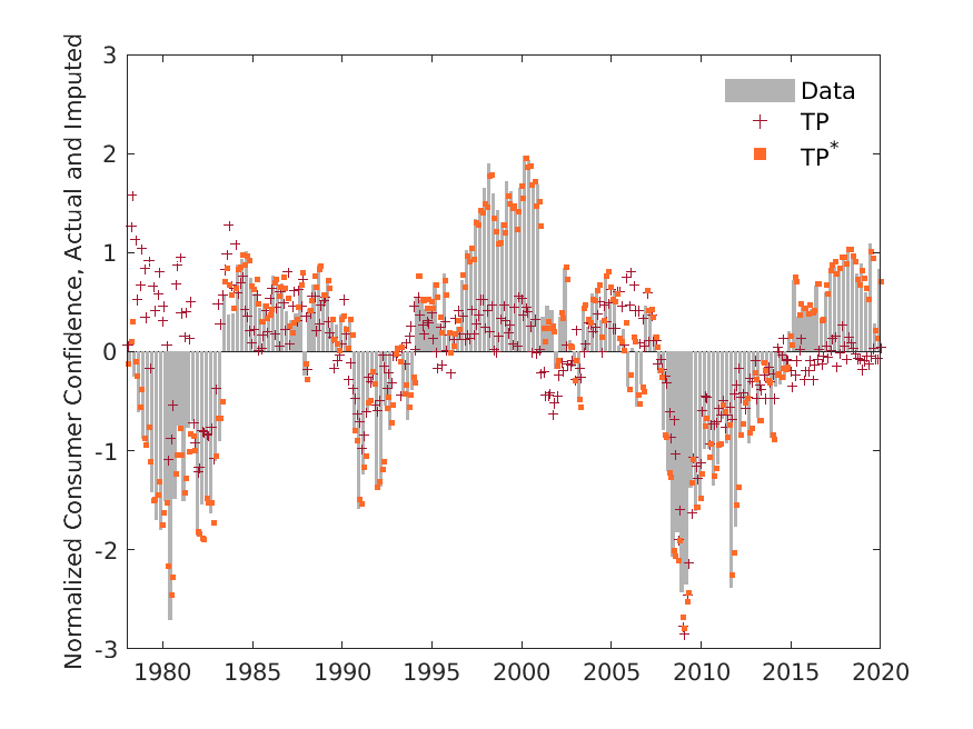
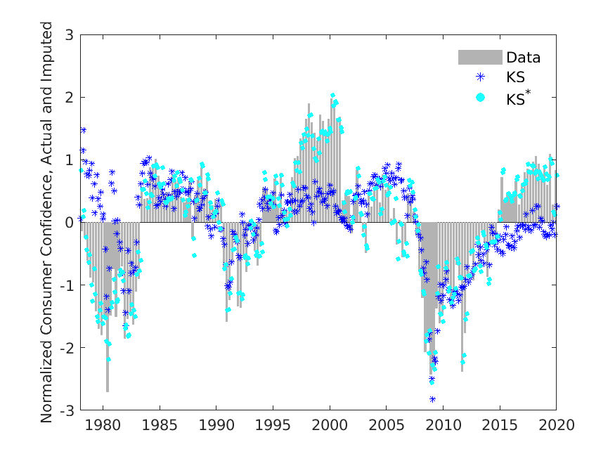
Figure 3: Monthly Consumer Confidence: Dynamic vs Static

The ”Data” bars are the true monthly values of Consumer Confidence. In a hypothetical experiment, it is assumed that quarterly values are missing - the monthly values are imputed. The imputed monthly values using the different procedures are denoted by the markers. The * superscript estimators model serially correlated residuals.

We evaluate imputation errors for the full sample and seven subsamples. van Buuren (2018, Chapter 2.6) emphasizes that imputation is not prediction and that the mean-squared error (MSE) is an uninformative metric for evaluating imputation methods. The argument, made in the context of estimating slope parameters when the data are incompletely observed, is that the evaluation would treat the missing values as random and sampling error should be taken into account. Our interest here is not estimation of the slope parameters but the missing values themselves, and in particular, whether they are centered around the true values. Though the variances of $\tilde{Y}_{H,s_{t}}$ are all downbiased because of omitting the variability of $\epsilon_{s_{t}}$, all procedures omit the same term.

Table 3: Mean-Squared Errors in Imputing Consumer Confidence

Notes: (i) TP: (PC-F,static); (ii) MLE-h (GLS-F, static), (iii) KS (KS), (iv) TP*: (PC-F, dynamic), (v) MLE*: (gls-F,dynamic); (vi) PC-GLS* (GLS-F, dynamic); (vii) KS* (KS, dynamic), (viii) CL (Chow-Lin, dynamic).

With this caveat in mind, Table 4.4 reports the MSE for four static and four dynamic estimates (with a suffix of ‘*’). The last column, ’CL’, refers to the Chow-Lin procedure which we treat as static. Of these, ks and ks* explicitly model the dynamics of $F$, while mle-h only accounts for heteroskedasticity. But the static imputation errors are much larger than the dynamic ones. In the full sample, dynamic imputation reduces the error by half and the difference is particularly pronounced in the subsamples before 2000. Consistent with the simulation results presented earlier, the gains from incorporating lagged information in $e_{Y}$ into the prediction model are much larger than using alternative estimators for $F$ and $\Lambda$. To reinforce this point, the bottom panel of Figure 3 plots ks (which is a filtered estimate) along with ks* (which is a smoothed estimate). Both use (8) for imputation and differ only in the estimator for $F$. The two are very similar, suggesting that the improvements are mainly due to information in lagged $Y$. In retrospect, this is not surprising because $\rho$ in this application is estimated to be well above 0.8.

The monthly data used to estimate the factors are seasonally adjusted. Seasonally unadjusted data are generally more volatile, but monthly seasonal variations are strictly periodic. To anticipate our analysis of seasonally unadjusted weekly data to follow, we add some seasonally unadjusted series to the monthly panel and repeat the counterfactual exercise. The dynamic procedures yield imputed values that closer to the observed values than the static procedures. However, we find that tp*, which does not directly model the idiosyncratic noise, is less sensitive to seasonal variations in the unadjusted data.

5 An Imputed Weekly CFNAI

In this section, we take the low frequency indicator $y$ to be CFNAI, a monthly diffusion index published by the Chicago Fed towards the end of each calendar month. The goal is to impute its weekly values $Y$. To this end, weekly data are collected and detrended for 13 real activity variables and 22 interest rates, exchange rates, and stock market variables from (monday) 01-01-1990 to (monday) 05-31-2021. The financial variables are quite collinear, and we eventually used all 13 real activity variables, consumer credit, two interest rates, a stock market index, and two money supply variables to form a 19 variable weekly panel with details given in the Appendix.

Analysis of weekly data can be challenging for several reasons. First, the sampling frequency is not constant. There are six years in our sample that have 53 weeks (1990, 1996, 2001, 2007, 2012, 2018), and there is at least one month in every year with five mondays. As the number of mondays in a month changes from month to month, $m_{t}$ varies with $t$. The problem is not conceptually difficult, but does require special handling of the details. The second issue is that the size of weekly panel is not only smaller than monthly panels like FRED-MD (McCracken and Ng 2016), but also less complete. In our case, 11 of the 19 variables have some missing values, some from outlier adjustments around the financial crisis. There are also ’ragged-edges’ once the sample is extended to the latest data available. Since the weekly panel is already rather small in size, we use tp to construct a complete data panel $X_{o}$ for the purpose of factor estimation. To focus on the historical weekly values of CFNAI, we exclude observations after COVID-19, giving $T=1566$ from 1990-01-01 to 2019-12-31.

The third issue is that some weekly series display strong seasonalities. The panel of seasonally unadjusted weekly data is better characterized by

$$X_{o}=F\Lambda_{o}^{{}^{\prime}}+\mathbb{S}+e_{X_{o}}$$

where $\mathbb{S}$ is a weekly seasonal component, assumed to be uncorrelated with the non-seasonal series specific noise $e_{X_{o}}$ and with the weekly factors, $F$. A weekly series can be more variable than the corresponding monthly series because of seasonality. An ideal seasonal adjustment would be to first estimate $\mathbb{S}$ and create a seasonally adjusted panel $X_{o}-\mathbb{S}$. But as discussed in Ng (2017); Guha and Ng (2022), off the shelf seasonal adjustment procedures developed for monthly/quarterly data tend not to be adequate for weekly data because the seasonal variations are not strictly periodic. The common approach, also taken in the construction of WEI and ECI, is to remove seasonality by taking 52 week differences when needed. Though this removes a good deal of the seasonal variations, it also creates large spikes because Thanksgiving and Easter in particular do not fall on the same week every year. Systems approaches that jointly model the weekly and monthly data would ideally also model these data irregularities, which is a daunting task.

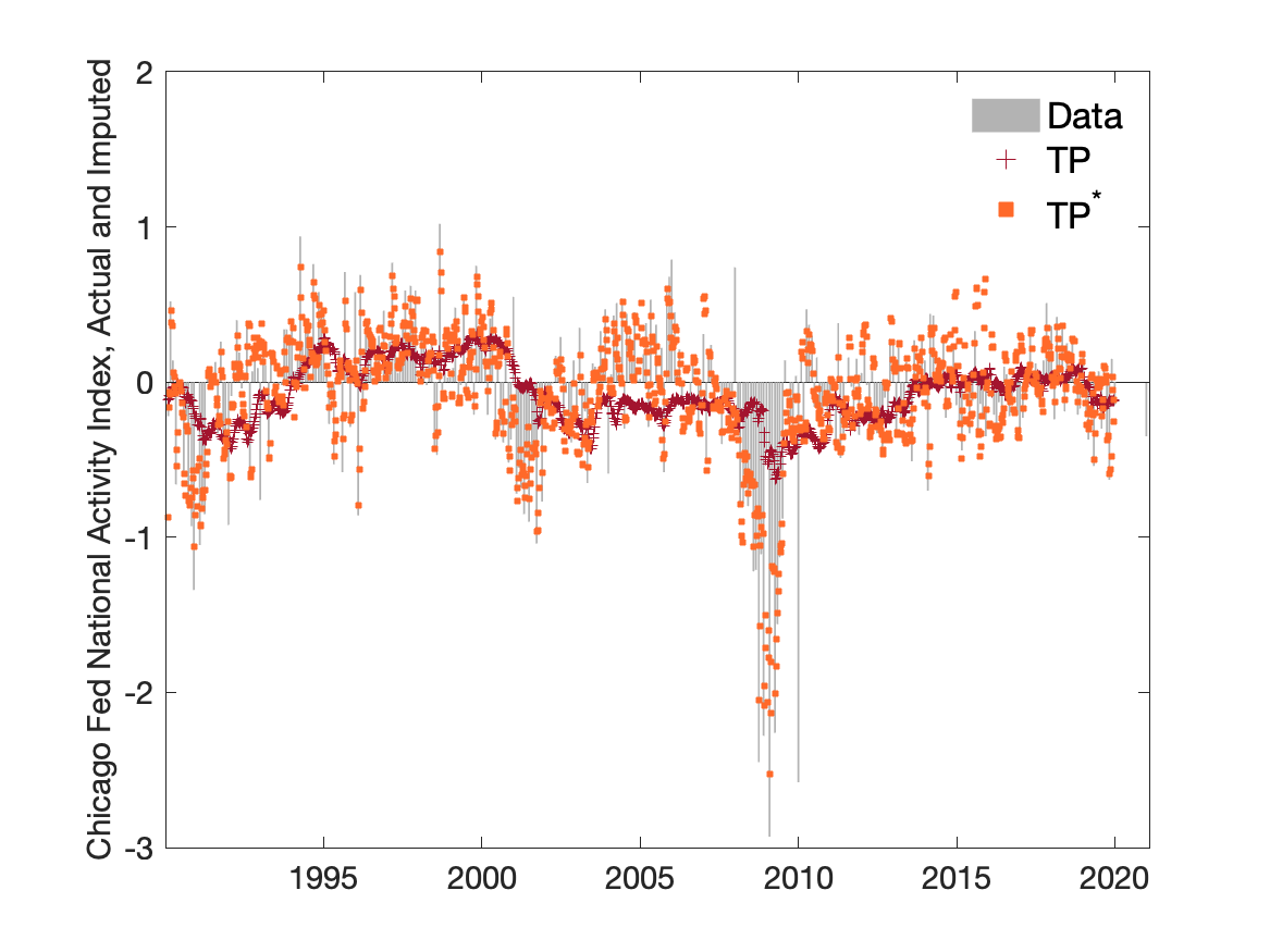
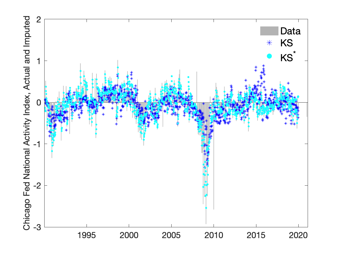
Figure 4: Weekly Chicago Fed National Activity Index: Dynamic vs Static

The ”Data” bars are the true monthly values of the Chicago Fed National Activity Index. Imputed ”missing” weekly values using the different procedures are denoted by the markers. The * superscript estimators model serially correlated residuals.

Our approach takes as starting point that so long as seasonal variations are idiosyncratic and serially uncorrelated, they play no role in imputation. We thus consolidate $\mathbb{S}$ with the idiosyncratic noise $e_{X_{o}}$ into a composite error. To smooth out the seasonal variations on the factor estimates and to make better use of information available, we expand $X_{o}$ to include three lags of each variable, which also increases the size of the panel from 19 to 76 series. The three factors in the expanded panel account for 62% of the variations in the data. The first weekly factor, which explains 35% of the variations in the data, loads most heavily on current and past values of unemployment claims. The second factor loads on current and past consumer credit, while the third factor loads on current and past oil price. Once the factors are estimated, we implement static or dynamic imputation. By construction, the imputed values in the last week of each month are the observed monthly values.

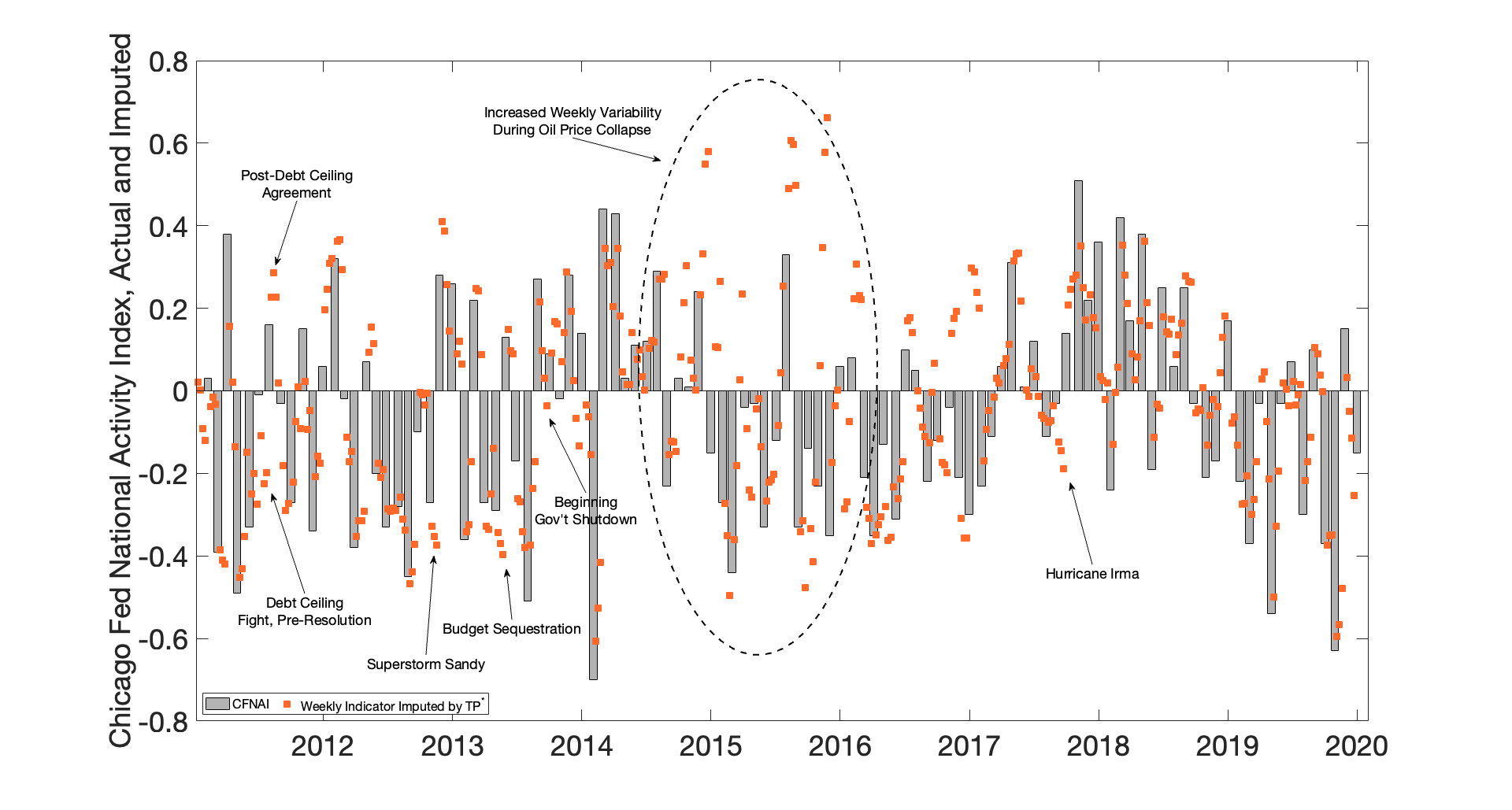
Figure 5: A Closer Look at Weekly Economic Activity 2011-2019

The top panel of Figure 4 compares the static and dynamic tp procedures (tp and tp*, respectively), and the bottom panel compares the static and dynamic ks procedures. The imputed values using the static tp model (dark red plus sign) is clustered closer to zero. The ks method shows only slightly more variation, and additionally appears to pick up some of the seasonal effects from the raw weekly data. Accounting for persistence of idiosyncratic component $Y$ yield significant improvements, as shown by the tp* (orange square) and ks* (light blue circle) procedures. While tp* only needs PC estimation of the factors, ks* also need to model the dynamics of the factors and the idiosyncratic noise. Because the seasonal component is now consolidated into the noise, the error variance is very difficult to estimate.

We obtain seven imputed measures of CFNAI but will focus on tp* and ks* to illustrate the difference between dynamic and static imputation. Our weekly imputed measures in general display lower volatility than the monthly measure, which is perhaps not surprising because the innovation at every $s_{t}$ is still set to the unconditional mean of zero. However, there are instances when the contribution of weekly information is notable. The dynamic estimation procedures pick up weekly readings distinct from the monthly data around a number of short-lived events events such as hurricanes, ice storms, and the collapse of Long-Term Capital Management. Consider for example weekly values of CFNAI in the wake of the 2014-2015 collapse in oil prices. As shown in Figure 5, the imputed weekly measures show greater variability than the monthly values during this time period. Historically such an unexpected decline would be expected to provide a sizable boost to economic activity, but, as documented in Baumeister and Kilian (2016), the boost to consumption was largely offset by the decline of investment in the oil sector. Contrary to previous episodes of oil price decline, the increased importance of shale production to the U.S. economy muddied the effect of the price drop. The monthly series captures the net effects while the imputed weekly values preserve these clashing forces. A similar phenomenon is reflected during pre- and post-debt ceiling debates (2011 and 2013).

6 Conclusion

A by-product of static factor analysis in the presence of missing values is imputation of those missing values. These imputed values are unconditionally unbiased without modeling the persistence of the idiosyncratic errors, accounting for the serial correlation provides better estimates of the target than static imputation. We have considered several ways by which residual serial correlation can be incorporated into imputation. However, the user still has many modeling choices to make: how to estimate the factors, and whether to use parametric state space modeling or a partial approach. Dynamic imputation complicates inference, and an assessment of the sampling uncertainty associated with the dynamic procedures remains a topic for future research. This is studied in Goncalves and Ng (2023) in the context of imputing counterfactual outcomes.

Appendix A: Estimators of Static Factors

OLS and GLS Based Principal Components

The PC estimator for complete data minimizes the objective function $\frac{1}{NT}\sum_{i=1}^{N}\sum_{t=1}^{T}(X_{it}-\Lambda_{i}^{\prime}F_{t})^{2}$ with respect to $F$ and $\Lambda$. Let $U$ and $V$ be singular vectors in the singular value decomposition $\frac{X}{\sqrt{NT}}=UDV^{\prime}$, where $D$ is a diagonal matrix of singular values arranged to be in decreasing order. Under the normalization that $F^{\prime}F/T=I_{r}$ and $\Lambda^{\prime}\Lambda$ is diagonal, the principal component (PC) estimates are defined by

$$(\tilde{F},\tilde{\Lambda})=(\sqrt{T}U_{r},\sqrt{N}V_{r}D_{r})$$

where $U_{r}$ and $V_{r}$ are the left and right singular vectors corresponding to the $r$ largest singular values collected in the diagonal entries of $D_{r}$. The PC estimates repeatedly perform OLS regressions of $X_{t}=(X_{1t},\ldots,X_{Nt})^{\prime}$ on the most recent estimates of $\Lambda=(\Lambda_{1},\ldots,\Lambda_{N})^{\prime}$, and of $X_{i}=(X_{i1},\ldots,X_{iT})^{\prime}$ on the most recent estimates of $F=(F_{1},\ldots,F_{T})^{\prime}$. The properties of $(\tilde{F},\tilde{\Lambda})$ are analyzed in Stock and Watson (2002a); Bai and Ng (2002); Bai (2003), among others.

Improvements to PC can be obtained even if $\Phi$, the misspecified idiosyncratic error variance, is not jointly estimated with $\Lambda$ as in maximum likelihood. One idea, noted in Boivin and Ng (2006) and others, is that PC estimation ignore the non-spherical error structure of the idiosyncratic errors and hence inefficient. Non-sphericalness can arise if the errors are serially correlated or heteroskedastic. Suppose that $e_{it}$ is a first order autoregressive process, $e_{it}=\rho_{i}e_{it-1}+\epsilon_{it}$, $\epsilon_{it}\sim(0,\sigma^{2}_{\epsilon_{i}}).$ If $F$ was observed, the efficient estimator of $\Lambda_{i}$ is a GLS regression of $X_{i}$ on $F$ which amounts to applying OLS to quasi-differenced $X_{it}$ and quasi-differened $F_{t}$:

$$[(1-\rho_{i}L)X_{it}]=[(1-\rho_{i}L)]F_{t}^{\prime}]\Lambda_{i}+\text{error}.$$ (9)

While controlling for serial correlation in $e_{it}$ is useful in estimation of $\Lambda$, accounting for heteroskedasticity by GLS is important for estimation of $F$. Breitung and Tenhofen (2011) suggest to update the PC estimate of $F$ using an estimate of $\Phi$. We will subsequently refer to the PC estimator that only accounts for heteroskedasticty as PC-GLS-h. If the $\Lambda$ estimates are also updated, it will be referred to as PC-GLS-har since it accounts for both heteroskedasticty and serial correlation. See Bai and Li (2012, Section 7) and Doz et al. (2012).

Quasi Maximum Likelihood Estimator

As the name suggests, estimators based on quasi maximum likelihood directly maximize a misspecified likelihood function. Bai and Li (2012, 2016) jointly estimate $\theta=(\Phi,\Sigma_{F},\Lambda)$ by maximizing the quasi-log-likelihood

$$\log L=\frac{1}{2N}\log|\Sigma_{X}(\theta)|-\frac{1}{2N}\text{tr}\bigg{(}S_{X}\Sigma_{X}^{-1}(\theta)\bigg{)}$$

where $\Sigma_{X}(\theta)=\Lambda\Sigma_{F}\Lambda+\Phi$ is the covariance matrix implied by the model, $\Sigma_{F}$ is the $r\times r$ covariance of $F$, and $S_{X}$ is the sample covariance of $X$. The misspecification is that a diagonal $\Phi$ is assumed for $\Sigma_{e}$ even when it is not diagonal. The estimator for $\Lambda$, say $\hat{\Lambda}$, solves the system of first order conditions with respect $\Lambda$, $\Phi=\text{diag}(\Sigma_{e})$, and $\Sigma_{FF}$. Assuming joint normality of $X$ and $F$, an infeasible projections estimator for $F$ under this framework can be defined as:

$$F_{t}^{p}=E_{\Theta}[F_{t}|X_{1},\ldots,X_{T}]=\bigg{(}\Sigma^{-1}_{F}+\Lambda^{\prime}\Phi^{-1}\Lambda\bigg{)}^{-1}\Lambda^{\prime}\Phi^{-1}X_{t}.$$

An alternative is the infeasible GLS estimator:

$$F^{GLS}_{t}=(\Lambda^{\prime}\Phi^{-1}\Lambda)^{-1}\Lambda^{\prime}\Phi^{-1}X_{t}.$$

The feasible analogs are obtained by plugging in MLE estimates for $\Lambda$ and $\Phi$ into (3). When $\Phi$ only allows for heteroskedasticity, we will refer to it as MLE-h. Bai and Li (2012, 2016) show that the estimator is more efficient than PC.

Accounting for Dynamics in $F$.

The static factors are identified in PC estimation by cross-section smoothing and ignores intertemporal information. The QMLE framework can be used to exploit information available in the dynamics of $F$. Let $\mathcal{X}=\text{vec}(X)$ and $\Sigma_{\mathcal{F}}$ be the matrix of autocovariances of the $rT\times 1$ vector $\mathcal{F}=\text{vec}(F^{\prime})$. A projections estimator that takes the dynamics of $F$ into account is $F^{p}_{t}=\mathbf{U}_{t}^{\prime}\mathcal{F}^{p}$ where $\mathbf{U}_{t}^{\prime}=(\iota_{t}\otimes I_{r})$, $\iota_{t}$ is the $t$-th column of $I_{T}$.,

$$\mathcal{F}^{p}=E_{\Theta}(\mathcal{F}|\mathcal{X}] = \bigg{(}\Sigma_{\mathcal{F}}^{-1}+(I_{T}\otimes\Lambda^{\prime}\Phi^{-1}\Lambda)\bigg{)}^{-1}\bigg{(}(I_{T}\otimes\Lambda^{\prime}\Phi)\bigg{)}\mathcal{X}.$$

Computation of of $\Sigma_{\mathcal{F}}$ requires a dynamic model for $\mathcal{F}$. If $\mathcal{F}$ is assumed to be a VAR of order $p$, the state space representation of $X$ is

$$X_{t} =\Lambda\mathcal{F}_{t}+\epsilon_{t} \epsilon_{t}\sim N\left(0,\Sigma_{\epsilon}\right)$$

$$\mathcal{F}_{t+1} =\mathcal{A}_{1}\mathcal{F}_{t}+\mathcal{A}_{2}\mathcal{F}_{t-1}+\dots+\mathcal{A}_{p}\mathcal{F}_{t-p+1}+\eta_{t} \eta_{t}\sim N\left(0,\Sigma_{\eta}\right)$$

Doz et al. (2011) use the Kalman smoother to obtain $\hat{\Sigma}_{\mathcal{F}}$ for an improved estimate of $F$. This, together with the OLS estimates $\hat{\Sigma}_{e}$ and $\hat{\Lambda}$ yields $\hat{F}_{t}=\mathbf{U}_{t}^{\prime}\hat{\mathcal{F}}^{p}$. We will refer to this hybrid estimator as PC-KS. State space models is fully parametric and is efficient if the assumptions are correct. Section 5.2 suggests a way to rewrite the observation and transition equations to accommodate serially correlated idiosyncratic error.

Data Appendix

Variable	Source
Electric Utility Output	Edison Electric Institute, WRDS
Raw Steel Production	American Iron and Steel Institute, WRDS
Rail Traffic: Total	Association of American Railroads, WRDS
Rail Traffic: Class 1 Intermodal Units	Association of American Railroads, WRDS
Rotary Rig Count	Baker Hughes, WRDS
Unemployment Insurance Claims: Initial	U.S. Department of Labor, WRDS
Unemployment Insurance Claims: Cont.	U.S. Department of Labor, WRDS
Redbook, Same Store Sales	Redbook Research Inc., WRDS
WTI Oil Price	Commodity Research Bureau
CRB Commodity Price Index	Commodity Research Bureau
Mortgage Application Survey: Avg Total Loan	Mortgage Bankers Association
Mortgage Application Survey: Market Index	Mortgage Bankers Association
US Fuel Sales to End Users	U.S. Energy Information Administration
Consumer Credit	Board of Governors of FRS
Commercial Paper	Board of Governors of FRS
3-Month Treasury	Board of Governors of FRS
C&I Loans, Large Banks / M1	Board of Governors of FRS
S&P Industrial / M1	Standard and Poor’s / BoG
S&P 500	Standard and Poor’s

References

- Antolin-Diaz et al. (2021) Antolin-Diaz, J., T. Drechsel, and I. Petrella (2021). Advances in nowcasting economic activity: Secular trends, large shocks and new data. mimeo, FRB Philiadelphia.
- Arminger and Sobel (1990) Arminger, G. and M. Sobel (1990). Pseudo-maximum likelihood estimation of mean and covariance stctures with missing data. Journal of the American Statistical Association 85:409, 195–203.
- Aruoba et al. (2009) Aruoba, S. B., F. X. Diebold, and C. Scotti (2009). Real-time measurement of business conditions. Journal of Business and Economic Statistcs 27, 417–247.
- Bai (2003) Bai, J. (2003). Inferential theory for factor models of large dimensions. Econometrica 71:1, 135–172.
- Bai and Li (2012) Bai, J. and K. Li (2012). Statistical analsyis of factor models of high dimension. Annals of Statistics 40, 436–465.
- Bai and Li (2016) Bai, J. and K. Li (2016). Maximum likelihood estimation and inference for approximate factor models of high dimension. Review of Economics and Statistics 98:2, 298–309.
- Bai and Ng (2002) Bai, J. and S. Ng (2002). Determining the number of factors in approximate factor models. Econometrica 70:1, 191–221.
- Bai and Ng (2019) Bai, J. and S. Ng (2019). Rank regularized estimation of approximate factor models. Journal of Econometrics 78-96, 212:1.
- Bai and Ng (2021) Bai, J. and S. Ng (2021). Matrix completion, counterfactuals, and factor analysis of missing data. Journal of the American Statistical Association 116:536, 1746–1763.
- Banbura et al. (2013) Banbura, M., D. Giannone, M. Modugno, and L. Reichlin (2013). Now-casting and the real-time data flow. In Handbook of Forecasting, Volume 2A, pp. 196–233. Elsevier.
- Banbura and Modugno (2014) Banbura, M. and M. Modugno (2014). Maximum likelihood estimation of factor models on datasets with arbitrary pattern of missing data. Journal of Applied Econometrics 29(1), 133–16–.
- Barigozzi and Luciani (2019) Barigozzi, M. and M. Luciani (2019). Quasi maximum likelihood estimation and inference of large approximation dynamic factor models. arXiv:1910.03821.
- Baumeister and Kilian (2016) Baumeister, C. and L. Kilian (2016). Forty years of oil price fluctuations: Why the price of oil may still surprise us. Journal of Economic Perspectives 30:1, 139–160.
- Baumeister et al. (2021) Baumeister, C., D. Levia-León, and E. Sims (2021). Tracking weekly state-level economic conditions. NBER Working Paper 29003.
- Boivin and Ng (2006) Boivin, J. and S. Ng (2006). Are more data always better for factor analysis. Journal of Econometrics 132, 169–194.
- Brave et al. (2019) Brave, S., R. Butters, and A. Justiniano (2019). Forecasting economic activity using mixed frequency bvars. International Journal of Forecasting 35:4, 1692–1707.