Quasilocalized charge approximation approach for the nonlinear structures in strongly coupled Yukawa systems

Abstract

Strongly coupled systems occupying the transitional range between the Wigner crystal and fluid phases are most dynamic constituents of the nature. Highly localized but strongly interacting elements in this phase posses enough thermal energy to trigger the transition between a variety of short to long range order phases. Nonlinear excitations are often the carriers of proliferating structural modifications in the strongly coupled Yukawa systems. Well represented by a laboratory dusty plasma, these systems show explicit propagation of nonlinear shocks and solitary structures both in experiments and in first principle simulations. The shorter scale length contributions remain absent at strong screening in present approximate models which nevertheless prescribe nonlinear solitary solutions that consequently lose their coherence in a numerical evolution of the system under a special implementation of the quasi-localized charge approximation formulation. The stable coherent structures self-consistently emerge following an initial transient in the numerical evolution which adapts QLCA approach to spatiotemporal domain for accessing the nonlinear excitations in the strong screening limit. The present $\kappa\sim 1$ limit of the existing Yukawa fluid models to show agreement with the experiment and MD simulations has therefore been overcome and the coherent nonlinear excitaitons have become characterizable up to $\kappa\sim 2.7$, before they becoming computationally challenging in present implementation.

I Introduction

Physical systems exhibiting a strongly coupled phase in the limit of potential energy of interaction exceeding the kinetic or random energy of particles are very effectively modelled by a highly charged minority dust species immersed in an electron-ion plasma. The deterministic configurational correlation between these highly charged species often dominates their response over the kinetic randomness. This most accessible example of a strongly coupled systems allows quantitative description of the possible solid and gaseous phases by only two parameters, namely, the coupling parameter $\Gamma=Z^{2}e^{2}/ak_{B}T$ and the screening parameter $\kappa=a/\lambda_{D}$, where $\lambda_{D}$ is the plasma Debye length, $a$ is inter-dust separation (Wigner-Seitz radius), $Z$ is dust charge multiplicity of the electronic charge $e$, $T$ is dust kinetic temperature and $k_{\rm B}$ is the Boltzmann constant. A vast range of strongly coupled systems modeled by this include dense astrophysical systems (Peng et al., 2007), warm dense matter, trapped ions (Dantan et al., 2010), ultracold neutral plasma (Killian et al., 2007), etc.

An intermediate state between the so called Wigner crystal (Wang et al., 2001) ($\Gamma>\Gamma_{\rm melting}$) phase and the gaseous phase ($\Gamma\sim 0$) remains the most challenging one. This is evident from the fact that a dynamic mean-free version of the random phase (gaseous) approximation (Hou et al., 2004, 2009; Kaw and Sen, 1998; Kaw, 2001), as well as a solid phase approach acknowledging particle correlation function $g(r)$ (Golden and Kalman, 2000; Donko et al., 2008) have been applied to this intermediate phase with limited success. In accounting for $g(r)$, a considerable localized stay of dust particles in their fragile (piecewise stable) macroscopic potential landscape is acknowledged just below $\Gamma_{\rm melting}$ closely resembling the phonon formulation applicable well above $\Gamma_{\rm melting}$. This Quasi-localized Charge Approximation (QLCA) is thus applied with a considerable success not only in linear perturbative limit (Golden and Kalman, 2000; Kalman et al., 2005) but finite prospects are also explored of its non-perturbative (Golden et al., 2009) applicability to the nonlinear excitations (Lee and Kalman, 2011).

In a laboratory setup, dusty plasmas exhibit both molten and crystelline phases of a strongly coupled system (Morfill and Ivlev, 2009). The linear excitations of the dust, namely the the longitudinal dust acoustic waves, and transverse shear modes are well explored by various theoretical models, such as the Generalized Hydrodynamics (GH)(Kaw and Sen, 1998; Kaw, 2001), thermodynamic approach(Khrapak and Thomas, 2015), $T^{\rm(eff)}$ model(Yaroshenko et al., 2010) and Quasi-localized Charge Approximation (QLCA) (Golden and Kalman, 2000; Khrapak et al., 2016; Kalman et al., 2000). In the weak screening regime $\kappa$ (= a/$\lambda_{D}$) $\leq$ 1 (where $a$ being the lattice constant and $\lambda_{D}$ being the debye length), the GH approach described not only of the longudinal modes but also reproduced the gap at long wavelengths, or the $k$ gap (Kaw and Sen, 1998; Kaw, 2001), of the transverse (shear) acoustic mode dispersion. The excitation in the strong screening limit ($\kappa\gg 1$) accessed by GH model however depart from the MD simulation dispersion (Ohta and Hamaguchi, 2000) as the original One Component Plasma (OCP) version of the GH model requires essential screening specific corrections both in the equation of state and the excess energy $u(\Gamma)$ which enter its phenomenological dispersion relation (Kaw and Sen, 1998; Kaw, 2001). On the other hand, linear dispersions in the strong coupling limit are successfully recovered under the QLCA formulation and the resulting dispersion (Golden and Kalman, 2000; Khrapak et al., 2016; Donko et al., 2008) remains in agreement with experiments (Nunomura et al., 2005) and MD simulations (Ohta and Hamaguchi, 2000; Khrapak et al., 2016; Donko et al., 2008; Kalman et al., 2000). The QLCA formulation, by accounting for a qasi-localized dust structure, omits dust diffusion to work in the infinite relaxation time limit ($\tau_{r}\rightarrow\infty$) of the phenomenological dispersion $\omega^{2}=c^{2}k^{2}-\tau_{r}^{-2}$ (Yang et al., 2017), hence excludes the $k$-gap of the transverse dispersion and access $k\rightarrow 0$ excitations. The nonlinear longitudinal excitations, which are subject of the present paper, are treated for the first time under QLCA formulation which besides being in agreement with GH solutions in weak screening limit Sharma et al. (2014); Boruah et al. (2016), allows access to the presently unexplored strong screening limit of the nonlinear excitations.

Despite its strength in treating the strong screening regime, the application of QLCA formulation to nonlinear excitations is limited by its intrinsically spectral form largely suitable to linear excitations. This barrier is overcome in the present treatment by adopting the recently developed excluded volume approximation (Khrapak et al., 2016) and its numerical implementation for evaluating the QLCA dynamical matrix in the spatiotemporal domain for ready applicability to nonlinear perturbations and exmining their stability with respect to temporal evolution. We have first shown that an analytical approximation of the QLCA dynamic matrix $D_{L}$(Golden and Kalman, 2000; Rosenberg and Kalman, 1997) in terms of excess energy (the OCP implementation), limited to weak screening limit, reproduces results available from the GH prescription. Applying QLCA formulation in its full capacity to the strong screening limit, we subsequently recover a strong departure of the nonlinear excitations from their weak screening counterparts. The nonlinear structures in this limit are shown to be characteristically distinct when compared to the OCP implementation of the formulation when the latter is nevertheless used to produce nonlinear solutions with relatively larger $\kappa$. The access to larger frequency, or shorter wavelength limit, where the OCP based descriptions, including the original GH dispersion as well as its QLCA counterpart, show strong limitation is now available by means of the presented excluded volume approximation of the QLCA dynamical matrix. The corresponding QLCA linear dispersion is shown to closely agree with the results of the MD simulation in this regime. In particular, the $\kappa\sim 1$ limit for the existing Yukawa fluid models to show agreement with the experiment and simulations has been overcome by the present QLCA prescription and agreement is now recoverable up to $\kappa\sim 2.7$.

The article is organized as follows. In Sec. II, the linear QLCA formulation is outlined beginning from a more general rotating frame version of it analyzed recently (Kumar and Sharma, 2021). The nonlinear approach to excitations with localization accounted for by QLCA formulation within the KdV framework as well as in a general pseudospectral nuemrical framework are presented in Sec. II.2 and Se. III, respectively, alongwith a description of isothermal dust compressibility in Sec. II.3. Impact of the localization on linear and nonlinear analytical solutions of the model is analyzed on KdV-prescribed and more general form of coherent perturbations in Sec. III and Sec. IV, respectively. Summary and conclusions are presented in Sec. VI

II Nonlinear QLCA theory for a strongly coupled Yukawa system

The QLCA theory has been successfully applied to study collective excitation of the liquid phase strongly coupled systems in a rotating (Kumar and Sharma, 2021) as well as non-rotating frame(Golden and Kalman, 2000). The microscopic equation of motion of the dust particle in a rotating frame, for the component $r_{i\mu}$ aligned to the direction $\mu~{}(=x,y)$,

$$\begin{split}m_{\rm d}\frac{\partial^{2}{r}_{i\mu}}{\partial t^{2}}=\sum_{j}{K}_{ij\mu\nu}r_{j\nu}-2m_{\rm d}\left[{\bf\Omega}\times\frac{\partial{\bf r}_{i}}{\partial t}\right]_{\mu}\\ -m_{\rm d}[{\bf\Omega}\times({\bf\Omega}\times{\bf r}_{i})]_{\mu}-\frac{\partial V}{\partial r_{\mu}}=0,\end{split}$$ (1)

where the second and third terms in the right-hand side are the Coriolis force and centrifugal force, respectively. The quantity V is the dust confinement potential whose gradient balances the corresponding component of the centrifugal force in the typical equilibrium condition (Kumar and Sharma, 2021). This equation can be reduced, in a non-rotating frame ($\Omega\rightarrow 0$), to a form given as (Golden and Kalman, 2000),

$$\begin{split}m_{\rm d}\frac{\partial^{2}{r}_{i\mu}}{\partial t^{2}}=\sum_{j}{K}_{ij\mu\nu}r_{j\nu},\end{split}$$ (2)

where the non-retarded limit of ${K}_{ij\mu\nu}$ defines the potential energy of the strongly coupled Yukawa fluid. The particles interact with each other through a shielded potential, namely, the Yukawa potential which is provided by the uncorrelated background plasma, given as,

$$\phi(|{\bf r}_{i}-{\bf r}_{j}|)=e^{-\kappa_{b}|{\bf r}_{i}-{\bf r}_{j}|}\frac{Z^{2}e^{2}}{|{\bf r}_{i}-{\bf r}_{j}|},$$ (3)

where the screening parameter $\kappa_{b}$ is defined by the uncorrelated background plasma pressure and self consistent electric field E = $\nabla\phi(|{\bf r}_{i}-{\bf r}_{j}|)$ between the negatively charged dust particles can be derived.

The well known linear QLCA results are recovered from equation for the linear perturbation eigenmodes $\xi_{{\bf k}\nu}(\omega)$ of $r_{i\mu}$ and an ensemble averaging of the collective coordinates Golden and Kalman (2000); Kalman et al. (2005),

$$[\omega^{2}\delta_{\mu\nu}-C_{\mu\nu}({\bf k},\omega)]\xi_{{\bf k}\nu}(\omega)=0,$$

where $C_{\mu\nu}$ contains the mean field and local field effects, produced by the random motion and the dust-dust correlation, respectively,

$$C_{\mu\nu}({\bf k},\omega)=\omega_{\rm pd}^{2}\left[\frac{k_{\mu}k_{\nu}}{k^{2}+\kappa_{b}^{2}}+\cal{D}_{\mu\nu}({\bf k},\omega)\right],$$ (4)

with $\omega_{pd}$ being the dust acoustic frequency. The central quantity in the QLCA, the dynamical matrix in three dimensions, given as,

$$D_{L,T}({\bf k})=\omega_{\rm pd}^{2}\int_{0}^{\infty}dr\frac{e^{-\kappa r}}{r}[g(r)-1]{\cal K}_{L,T}(kr,\kappa r),$$ (5)

includes dust-dust correlation effects, as this is a functional of the equilibrium pair correlation function (PCF). Clearly, in the absence of any correlations $g(r)\rightarrow 1$ at all values of $r$, the linear QLCA approach begins to provide the mean-field, or random-phase approximation results ($\cal{D}_{\mu\nu}$ = 0). Since the desired strong coupling effect enter the formulation predominantly by means of the functional $D_{L,T}$, the nonlinear treatment presented here exploits its adoptation to the spatiotemporal domain while retaining the contributions from the coupling of the individual modes, exclusively achievable under a nonlinear pseudospectral framework(Fornberg, 1998) .

II.1 Strong coupling in explicit QLCA approach

There remain two options for including the strong coupling effects applicable to two different states of the dust medium, namely, the strong coupling without localization ($g(r)=1$) and the stronger coupling with finite localization ($g(r)\neq 1$). While the first is achievable by an ad hoc inclusion of strong coupling effects in the pure fluid approach without invoking the QLCA framework since there is no localization, however the second essentially requires QLCA framework as $g(r)\neq 1$ and it is impossible to reduce QLCA to the fluid theory for finite localization limit without reasonable approximations. This puts a natural limit on applicability of the first kind of approach to strongly coupled systems, since when coupling is sufficiently strong finite localization must emerge and the second kind of approach begins to be applicable (Kalman et al., 2005; Donkó et al., 2003). We have summarized the (linear) dispersions from treatments belonging to the first option in Appendix VII their relation will be discussed with the nonlinear results obtained by us using the explicit QLCA approach ($g(r)\neq 1$) which show distinction with the existing nonlinear results.

In the limit where $D_{L}$ is a function of excluded volume parameter R($\Gamma$,$\kappa$) (Khrapak et al., 2016), it is derived by choosing a simple but reasonable valid approximation on $g(r)$, i.e., $g(r)=1$ for $r>R$ and $g(r)=0$ otherwise, or in a long-wavelength limit, as,

$$D_{L}=-\omega^{2}_{0}(k)+\omega_{\rm pd}^{2}e^{-kR}\left[(1+kR)\left(\frac{1}{3}-\frac{2\cos{kR}}{k^{2}R^{2}}\right.\right.$$

$$\left.\left.+\frac{2\sin{kR}}{k^{3}R^{3}}\right)-\frac{\kappa^{2}}{\kappa^{2}+k^{2}}\left(\cos{kR}+\frac{\kappa}{k}\sin{kR}\right)\right]$$

(6)

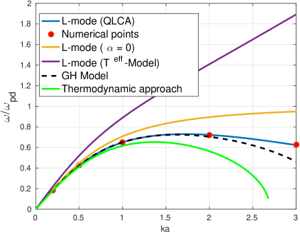
Figure 1: Analytical (blue lines) and numerical (red dot points) longitudinal wave dispersion relation for the charged dust fluid with values $\Gamma$ = 185, $\kappa$ = 1.0, and excluded volume $R(\kappa)$ = 1.1. The dispersion relation represented by the yellow and purple lines are obtained from a weakly coupled limit ($D_{L}$ = 0) and from a $T^{\rm(eff)}$ model, respectively. The green curve and dash line correspond to the dispersion relation calculated using the thermodynamic approach and GH model, respectively, for the parameters $\kappa$ = 1 and $\Gamma$ = 207.

The effective parameter for the excluded volume, $R(\Gamma,\kappa)$, is function of the system state variables, $\kappa$ and $\Gamma$, evaluated using the expression of a system correlation energy. A simple explicit expression for this excluded volume parameter, $R\approx 1+\frac{\kappa}{10}$, has been calculated for a weak screening regime (Khrapak, 2017). In Fig. 1 we have compared the strong-coupling limit linear QLCA dispersion, Eq. (4), with the dispersion in Eq. (41), Eq. (42) and GH model (Kaw, 2001) which admit the strong coupling effects using $T^{\rm(eff)}$, thermodynamic functions and viscoelastic coefficients, respectively, but no explicit localization. The QLCA dispersion relation in Eq. (4) as computed under excluded volume approximation for the case using $\Gamma$ $\approx$ 180, $\kappa$ = 1 and R = 1.1 as in Ref. (Khrapak et al., 2016) is plotted in Fig. 1 using blue line which is in agreement with Ref. (Khrapak et al., 2016). The red dots superimposed on the plot are numerically computed dispersion relation by solving, using pseudo-spectral method, the full nonlinear set of QLCA equations under the same approximation showing excellent agreement with linear model at small amplitudes. While the yellow curve saturating to dust acoustic frequency $\omega_{\rm pd}$ represents the pure random-phase (fluid-limit) dispersion relation, a contrasting behavior with respect to QLCA dispersion is shown by the dispersion plotted with purple line which is the strong coupling dispersion (41) not admitting localization. While the green curve, obtained from the Eq.(42) shows correspondence with the QLCA model (blue curve/red dots) at very long wavelength regime ($ka<$ 1.0), it shows continuous deviation from the QLCA dispersion at relatively higher mode number (k $\geq$ 1.0), as can be seen form the Fig. 1. Note that both the analytical dispersion and the numerical solutions (red dots) obtained from full nonlinear QLCA model implemented by us (red dots in Fig. 1) show agreement also with the Molecular Dynamical(MD) simulations (Donko et al., 2008; Khrapak et al., 2016) as well as the experimental studies (Bandyopadhyay et al., 2007). While the GH model provides good agreement with the QLCA based model at long wavelengths and weak screening limit, it requires presently unavailable corrections for agreement with shorter wavelength and strong screening limit of the dispersion relation recovered in MD simulations Kaw (2001). Access to this limit is additionally shown to be possible by a numerical implementation of $D_{L}$ under the QLCA framework where a more sophisticated form of $g(r)$, derived from MD simulation data, can be used rather than the excluded volume approximation. Results from this implementation are shown to make the comparison with GH model possible up to larger $k$ values in Fig. 2 where

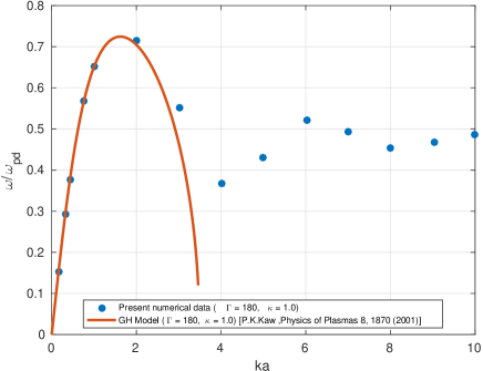
Figure 2: The red curve crossespond to the dispersion relation obtained from the GH model (Kaw, 2001) and the blue dots are plotted using QLCA based model, for same parameter values, $\Gamma$ = 180 and $\kappa$ = 1.0.

the radial pair correlation function $g(r)$ used in our pseudospectral computations is obtained from the MD simulation data adopted from Ref. (Khrapak et al., 2016). This yields the expression for $D_{L}$-matrix,

$$D_{L}(k)=\omega^{2}_{pd}[(-0.568+0.3149\cos(0.431k)+$$

$$0.056\sin(0.431k)+0.187\cos(0.862k)$$

$$+0.058\sin(0.862k)+0.0511\cos(1.293k)$$

$$+0.044\sin(1.293k)-0.00016\cos(1.724k)$$

$$-0.025\sin(1.72k)+0.0079\cos(2.155k)$$

$$-0.0090\sin(2.155k))]$$ (7)

which is also plotted in Fig. 3 with state parameters $\Gamma$ = 180 and $\kappa$ = 1.0.

While, as shown in Fig. 2, the GH Model and QLCA predict an identical dispersion relation in a long-wavelength ($ka\leq$ 2) limit, in a relatively short wavelength limit the present QLCA based numerical simulations successfully reproduce the oscillatory behavior which is characteristically observed in various theoretical studies (Khrapak et al., 2016; Donko et al., 2008), MD simulations (Mokshin et al., 2022) and experiments (Zhdanov et al., 2003; Nunomura et al., 2005). It is therefore clear that the result from the presently available OCP version of the GH model are not a reliable predictor for the short wavelength (high $k$) excitations. The corresponding $D_{L}(k)$ plotted in Fig. 3 shows that in the long wavelength regime (small $k$) the $D_{L}(k)$ has a variation which corresponds to the $g(r>R)\simeq$ 1 as approximated by the excluded volume prescription Khrapak et al. (2016). Under this approximation the large $r$ contribution to the wave dynamics dominates over the local interactions. At sufficiently shorter wavelengths (large $ka$), the strength of $|D_{L}|$ increases considerably, meaning that the structural effect contribution (i.e., $g(r)$ featuring multiple peaks in Ref. Khrapak et al. (2016)) to the wave dynamics increase significantly, an effect uniquely accounted for by the QLCA formulation.

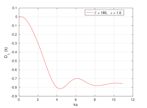
Figure 3: The plot of $D_{L}$-matrix using equation (7) which is obtained from the MD data and dispersion relation given in (Khrapak et al., 2016) with $\kappa$ = 1.

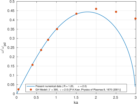
Figure 4: The blue curve crossespond to the dispersion relation obtained from the GH model (Kaw, 2001), $\Gamma$ = 395 and $\kappa$ = 2.0 and the blue dots are plotted using QLCA based model equation (4) for value, R=1.20 and $\kappa$ = 2.0.

For the shorter wavelength excitations, however, the discrepancy between the QLCA simulation based predictions (blue dots) and those of the GH model (solid curve) becomes significant. Remarkably, the excluded volume approximation, which uses a simplified step function like profile for the $g(r)$, still produces reasonably good correction to the linear dispersion, as in Fig. 1, and prescribes frequency values that recover from their steep drop at larger $k$, to instead saturate to the Einstein frequency Wong et al. (2017); Donko et al. (2008). This also remains the reason for a relatively better agreement between even approximate linear QLCA results and the MD simulation data. The comparison between the dispersions from GH and QLCA (excluded volume) for an additional case with higher screening parameter $\kappa=2.0$ is done in Fig. 4. In both cases the QLCA results remain in agreement also with MD simulations (Ohta and Hamaguchi, 2000) (not reproduced here) up to $ka\sim 3$.

II.2 Nonlinear excitations of a strongly coupled localized phase dusty plasma

The central idea of localization involves the macroscopic variables obtained from the ensemble averaged particle equations. For a nonlinear approach it is however required that the averages are done over spatiotemporal functions rather than their Fourier transformations. We therefore let the fluid conservation equations represent the evolution of these ensemble averages. We however acknowledge the presence of a spatial ordering of the dust sites by allowing the dynamical matrix $D_{L,T}$ (determining mechanical response of the system) to be computed via the grain-grain correlation energy which changes based on the strain in spatial ordering, in addition to the routine (random phase) response arising from the associated background plasma compression.

This ensemble averaged (macroscopic) momentum equation has same form as Eq. (LABEL:momentum-balance-rpa),

$$\begin{split}\frac{\partial{u}_{{\rm d}x}}{\partial t}+({\bf u}_{{\rm d}}\cdot\nabla){u}_{{\rm d}x}=\frac{q_{\rm d}}{m_{\rm d}}{E}_{x}-\frac{1}{m_{d}n_{d}}\frac{\partial P_{di}}{\partial x},\end{split}$$ (8)

where the dust kinetic energy is neglected because of being a few orders smaller than the representative strong coupling term $\frac{\partial P_{di}}{\partial x}$. Similarly, the macroscopic particle continuity equation obtained by ensemble averaging over the dust sites is,

$$\frac{\partial n_{dx}}{\partial t}+\frac{\partial}{\partial x}(n_{dx}u_{dx})=0.$$ (9)

Separate from the electric field $E_{x}$ produced by plasma species, the second term in the RHS of Eq. (8) accounts for the electrostatic field produced by the collective shift of the dust particles from their localized positions which must be predominantly restored by the dust structure, rather than purely by $E_{x}$. The term is therefore representable as a product of the density gradient produced and a force per unit density gradient. The latter is a rather sophisticated, localization-based, isothermal dust compressibility, treated further, both analytically and numerically, in Sec. II.3. It can be noted that, by construction, this new contribution must vanish if (i) there is no structured background dust distribution (i.e., if $g(r)\rightarrow 1$) and/or (ii) if these is no dust density perturbation with respect to this uniform structured dust background (i.e., if $\partial n_{d}/\partial x=0$). The Eq. (8) can therefore be written as,

$$\frac{\partial{u}_{dx}}{\partial t}+{u}_{dx}\frac{\partial{u}_{dx}}{\partial x}=-\frac{q_{d}}{m_{d}}\frac{\partial\phi}{\partial x}-\alpha\frac{1}{n_{d}}\frac{\partial n_{d}}{\partial x}.$$ (10)

where $\alpha_{c}=\frac{1}{m_{d}}\frac{\partial P_{di}}{\partial n_{d}}$ is the isothermal compressibility of the dust. Up on normalization, Eq. (10) takes the form,

$$\frac{\partial{u}_{dx}}{\partial t}+{u}_{dx}\frac{\partial{u}_{dx}}{\partial x}=\mu\frac{\partial\phi}{\partial x}-\tilde{\alpha}\frac{1}{n_{d}}\frac{\partial n_{d}}{\partial x},$$ (11)

and the normalized Poisson equation becomes,

$$\frac{\partial^{2}\phi}{\partial x^{2}}=\frac{1}{\mu}\left[n_{d}+n_{e}-n_{i}\right],$$ (12)

are now taken to be normalized. where we have $\mu=\frac{Z_{d}T_{i}}{m_{d}a^{2}\omega^{2}_{pd}}$, $\tilde{\alpha}=\alpha/\omega_{\rm pd}^{2}a^{2}$, $\delta_{e}=n_{e0}/Z_{d}n_{d0}$, $\delta_{i}=n_{i0}/Z_{d}n_{d0}$, $n_{e}=\delta_{e}(\sigma_{i}\phi)$, $n_{i}=\delta_{i}(-\phi)$ and $\sigma_{i}$ = $T_{i}/T_{e}$, while the equilibrium dust density $n_{d0}$, the ratio $T_{i}/e$, inverse dust acoustic frequency $\omega_{\rm pd}^{-1}$, and mean dust separation $a$ are used as normalizations for the density, potential, time and length, respectively. Eq. (11)-(12) along with the continuity Eq. (9) constitute a nonlinear model. Subject to an accurate representation of $\alpha$ in temrs of $D_{L}$, this can either be solved numerically, as done by means of the pseudospectral simulation procedure in the present work, or in a rather approximate (and routine) analytical procedure of the reductive perturbation theory (Davidson, 2012) (duly done in Sec. II.2.1, obtaining the associated KdV equation and its solutions).

The methodology followed here is to first obtain the solutions of the nonlinear KdV equation and use them as initial profiles in our spatiotemporal pseudospectral numerical evolution which covers additional, previously uncovered, parameter regime. More general initial profiles are numerically evolved after this analysis.

II.2.1 Derivation of the KdV equation for a strongly coupled fluid

In order to obtain the KdV equation (Davidson, 2012) for this system, we first introduce slow variable $\zeta$ and $\tau$, given by,

$$\zeta=\epsilon^{1/2}(x-v_{0}t),~{}~{}~{}~{}\tau=\epsilon^{3/2}t,$$ (13)

where $\epsilon$ is a smallness parameter measuring the weakness of the perturbation and $V_{0}$ represent the phase velocity of the DAW. In terms of $\zeta$ and $\tau$ the equations become,

$$\epsilon^{3/2}\frac{\partial n_{d}}{\partial\tau}-V_{0}\epsilon^{1/2}\frac{\partial n_{d}}{\partial\zeta}+\epsilon^{1/2}\frac{\partial n_{d}u_{d}}{\partial\zeta}=0,$$ (14)

$$\begin{split}\epsilon^{3/2}\frac{\partial u_{d}}{\partial\tau}-V_{0}\epsilon^{1/2}\frac{\partial u_{d}}{\partial\zeta}+\epsilon^{1/2}u_{d}\frac{\partial u_{d}}{\partial\zeta}=\mu\epsilon^{1/2}\frac{\partial\phi}{\partial\zeta}\\ -\frac{\alpha}{n_{d}}\frac{\partial n_{d}}{\partial\zeta},\end{split}$$ (15)

and

$$\begin{split}\epsilon^{3/2}\frac{\partial^{2}\phi}{\partial\zeta^{2}}=\frac{1}{\mu}\Bigg{\{}\delta_{e}\left[1+\sigma_{i}\phi+\frac{1}{2}\sigma^{2}_{i}\phi^{2}+..\right]\\ -\delta_{i}\left[1-\phi+\frac{1}{2}\phi^{2}+..\right]+n_{d}\Bigg{\}}.\end{split}$$ (16)

We can now expand the variables $n_{d}$, $u_{d}$ and $\phi$ in the power series of $\epsilon$,

$$\begin{split}n_{d}=1+\epsilon n^{(1)}_{d}+\epsilon^{2}n^{(2)}_{d}+...........\\ u_{d}=\epsilon u^{(1)}_{d}+\epsilon^{2}u^{(2)}_{d}+...........\\ \phi=\epsilon\phi^{(1)}+\epsilon^{2}\phi^{(2)}+...........\end{split}$$ (17)

Substituting Eq. (17) into the Eq. (15), (14) and (16), and equating coefficients of $\epsilon^{3/2}$, we get, to lowest order

$$-V_{0}\frac{\partial n^{(1)}_{d}}{\partial\zeta}+\frac{\partial u^{(1)}_{d}}{\partial\zeta}=0,$$ (18)

$$-V_{0}\frac{\partial u^{(1)}_{d}}{\partial\zeta}+\alpha\frac{\partial n^{(1)}_{d}}{\partial\zeta}-\mu\frac{\partial\phi^{(1)}}{\partial\zeta}=0,$$ (19)

and

$$-\frac{h_{1}}{\mu}\phi-\frac{1}{\mu}n^{(1)}_{d}=0,$$ (20)

where $h_{1}$ = $(\sigma_{i}\delta_{e}+\delta_{i})$ and $\kappa^{2}$ = $\frac{h_{1}}{\mu}$ = $\frac{a^{2}}{\lambda^{2}_{D}}$. Consequently the Eq. (20) becomes,

$$-\kappa^{2}\phi-\frac{1}{\mu}n^{(1)}_{d}=0,$$ (21)

After integrating and re-arranging terms, the following linear expressions are obtained,

$$u^{(1)}_{d}=-\frac{\mu V_{0}}{(V^{2}_{0}-\alpha)}\phi^{(1)},$$ (22)

$$n^{(1)}_{d}=-\frac{\mu}{(V^{2}_{0}-\alpha)}\phi^{(1)},$$ (23)

and

$$V_{0}=\left(\frac{\mu}{h_{1}}+\alpha\right)^{1/2}.$$ (24)

Eq. (24) represents the phase velocity of the dust acoustic wave as a function of $\alpha$.

Similarly, equating coefficients of $\epsilon^{5/2}$ from Eq. (15), (14) and that of $\epsilon^{2}$ from Eq. (16), the following equations are obtained,

$$\frac{\partial n^{(1)}_{d}}{\partial\tau}-V_{0}\frac{\partial n^{(2)}_{d}}{\partial\zeta}+\frac{\partial u^{(2)}_{d}}{\partial\zeta}+\frac{\partial u^{(1)}_{d}n^{(1)}_{d}}{\partial\zeta}=0,$$ (25)

$$\begin{split}\frac{\partial u^{(1)}_{d}}{\partial\tau}-V_{0}\frac{\partial u^{(2)}_{d}}{\partial\zeta}+\alpha\frac{\partial n^{(2)}_{d}}{\partial\zeta}-\alpha n^{(1)}_{d}\frac{\partial n^{(1)}_{d}}{\partial\zeta}\\ +u^{(1)}_{d}\frac{\partial u^{(1)}_{d}}{\partial\zeta}-\frac{\partial\phi^{(2)}}{\partial\zeta}=0,\end{split}$$ (26)

and

$$\begin{split}\frac{\partial^{2}\phi}{\partial\zeta^{2}}-\left(\frac{h_{1}}{\mu}\right)\phi^{(2)}+\left(\frac{h_{2}}{2\mu}\right)(\phi^{(1)})^{2}-\frac{1}{\mu}n^{(2)}_{d}=0,\end{split}$$ (27)

where $h_{2}$ = ($\delta_{i}-\delta_{e}\sigma_{i}^{2}$). Eliminating $u^{(2)}_{d}$, $n^{(2)}_{d}$ and $\phi^{(2)}$ from Eq. (25)-(27) and making use of Eq. (22)-(24), we find that $\phi^{(1)}$ satisfies the well known KdV equation,

$$\begin{split}\frac{\partial\phi^{(1)}}{\partial\tau}+A\phi^{(1)}\frac{\partial\phi^{(1)}}{\partial\zeta}+B\frac{\partial^{3}\phi^{(1)}}{\partial\zeta^{3}}=0,\end{split}$$ (28)

where the nonlinear coefficient $A$ and the dispersion coefficient $B$ are given by,

$$\begin{split}A=\left[\frac{\mu\alpha}{2V_{0}(V^{2}_{0}-\alpha)}-\frac{3\mu V_{0}}{2(V^{2}_{0}-\alpha)}+\frac{(V^{2}_{0}-\alpha)h_{2}}{2V_{0}h_{1}}\right]\end{split}$$ (29)

$$\begin{split}B=\frac{(V^{2}_{0}-\alpha)\mu}{2V_{0}h_{1}}\end{split}$$ (30)

with $h_{1}=(\sigma_{i}\delta_{e}+\delta_{i})$ and $h_{2}=(\delta_{i}-\sigma^{2}_{i}\delta_{e})$.

Eq. (28) can be solved by separation of variables, giving a solution in the laboratory frame as,

$$\begin{split}\phi(x,t)=\phi_{m}\text{sech}^{2}\left[\frac{\eta}{\Delta}\right],\end{split}$$ (31)

where

$$\begin{split}\phi_{m}=\frac{3U_{0}}{A}~{}~{}{\rm and}~{}~{}\Delta=\sqrt{\frac{4B}{U_{0}}},\end{split}$$ (32)

are the amplitude and width of the soliton, respectively, $\eta$ is a coordinate in the laboratory frame, and $U_{0}$ is the normalized velocity of the solitary wave. In the limit of $\alpha$ = 0, these coefficients reduce to well know results, A = $\frac{V^{3}_{0}}{2}\left(h_{2}-\frac{3}{V^{4}_{0}}\right)$, B = $\frac{V^{3}_{0}}{2}$, which correspond to the weak coupling limit of the dusty plasma (Shukla and Mamun, 2015).

II.3 Computation of isothermal dust compressibility from QLCA basics

For treating the general high screening regime of the nonlinear solutions, as central to the present paper, we will be using the more accurate form (6) of the dynamical matrix $D_{L,T}$. However, as presented below, the derivation of $D_{L,T}$ in the analytical form is possible in the weak screening limit to be compared against the nonlinear results from the GH model Sharma et al. (2014) which uses, and is limited to, the weak screening limit. For this purpose, one might use relationship of $\alpha$, for example, with the systems correlation energy (Hou et al., 2004, 2009). In the long-wavelength regime ($ka\leq 2$) as considered in the present case, a model simpler than involving the spectral representations (6) or (7) of $D_{L}$ is adopted here for $\alpha$ which essentially reproduces the more general QLCA results presented further below and therefore is equivalent to it (Hou et al., 2009). This is realizable because $\alpha$ = $\lim_{k\to 0}D_{L}/k^{2}$ (Golden and Kalman, 2000; Hou et al., 2009) and as long as $g(r)$ does not vary significantly with $\kappa$, $D_{L}$ - matrix remains suitably expressible in term of correlation energy and its derivative, given as (Rosenberg and Kalman, 1997; Golden and Kalman, 2000),

$$D_{L}({k\to 0})=\frac{4}{45}\omega^{2}_{pd}\left[1-\kappa\frac{\partial}{\partial\kappa}+\frac{3}{4}\kappa^{2}\frac{\partial}{\partial\kappa^{2}}\right]\frac{E_{c}(\kappa)}{T_{d}\Gamma}k^{2}.$$ (33)

Here $E_{c}$ is the grain-grain correlation energy which can be obtained analytically under the long-wavelength limit (Rosenberg and Kalman, 1997; Golden and Kalman, 2000) for a Yukawa fluid, as,

$$\frac{E_{c}}{T_{d}}=a(\kappa)\Gamma+b(\kappa)\Gamma^{1/3}+c(\kappa)+d(\kappa)\Gamma^{-1/3},$$ (34)

where the coefficient up to order $\kappa^{4}$ are given by,

$$a(\kappa)-\frac{\kappa}{2}=-0.899-0.103\kappa^{2}+0.003\kappa^{4}$$

$$=a_{0}+a_{2}\kappa^{2}+a_{4}\kappa^{4},$$

$$b(\kappa)=0.565-0.026\kappa^{2}-0.003\kappa^{4}=b_{0}+b_{2}\kappa^{2}+b_{4}\kappa^{4},$$

$$c(\kappa)=-0.207-0.086\kappa^{2}+0.018\kappa^{4}=c_{0}+c_{2}\kappa^{2}+c_{4}\kappa^{4},$$

$$d(\kappa)=-0.031-0.042\kappa^{2}-0.008\kappa^{4}=d_{0}+d_{2}\kappa^{2}+d_{4}\kappa^{4},$$

The expression for the $\alpha$ can be obtained by using the value of these coefficients in the equation (34) and then using Eq. (33) (Rosenberg and Kalman, 1997),

$$\alpha(\kappa,\Gamma)=\lim_{k\to 0}D_{L}(k)/k^{2}\approx\frac{4}{45\Gamma}\left[\left(a_{0}+a_{2}\frac{\kappa^{2}}{2}\right.\right.$$

$$\left.\left.+6a_{4}\kappa^{4}\right)\Gamma+\left(b_{0}+b_{2}\frac{\kappa^{2}}{2}+6b_{4}\kappa^{4}\right)\Gamma^{1/3}+\right.$$

$$\left.\left(c_{0}+c_{2}\frac{\kappa^{2}}{2}+6c_{4}\kappa^{4}\right)+\left(d_{0}+d_{2}\frac{\kappa^{2}}{2}+6d_{4}\kappa^{4}\right)\Gamma^{-1/3}\right].$$

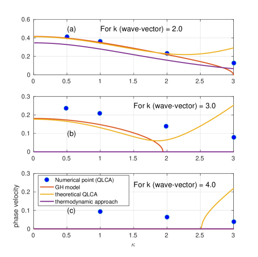
Figure 5: The variation of the linear phase velocity of the DAW with $\kappa$, (a) for fix value of $k$ = 2.0, (b) for fix value of $k$ = 3.0 and (c) for fix value of $k$ = 4.0. The red, yellow and violet curve crossespond to the results of the GH model, analytical QLCA based model and thermodynamic approach, respectively. The numerical blue points are plotted using QLCA based model.

One finds, to leading order in $\Gamma$ (Golden and Kalman, 2000),

$$\alpha(\kappa)=-0.0799-0.0046\kappa^{2}+0.0016\kappa^{4}$$ (36)

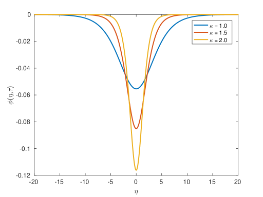
Figure 6: The variation of the negative solitary potential profile with $\kappa$ in the analytical QLCA limit (equivalent to GH results), for $h_{1}$ = 4, $h_{2}$ = 3.9, $U_{0}$ = 0.1 and inidicated $\kappa$ values.

This dependence of $\alpha$ on parameters $\Gamma$ and $\kappa$ defines the effects of dust-dust correlation in a Yukawa system viz. dusty plasma. Since $\alpha(\Gamma,\kappa)<0$, phase velocity of the dust acoustic wave in a strongly coupled limit given by Eq. (24) is reduced (Rosenberg and Kalman, 1997) as presented in Fig. 5. The nonlinear effects in the strongly coupled Yukawa system treated here under the QLCA theory can now enter the KdV equation through the coefficients $A$ and $B$ which are also the functions of $\alpha(\Gamma,\kappa)$.

III Numerical pseudo-spectral computation procedure and nonlinear coherent excitations

The spatiotemporal domain rather than the spectral (Fourier) domain is adopted for computationally solve the full nonlinear model described by the set of fluid equations (9)-(12), via a full nonlinear pseudo-spectral approach in which the spatial and temporal discretization are possible using the independent variables $k$ and $t$, respectively, yet, suitably providing the final solutions in the spatiotemporal domain $x$-$t$. The nonlinear term is calculated by implementing the 2/3-truncate rule in order to avoid the aliasing error (Coutsias et al., 1989). After due verification of the numerical simulation procedure for standard nonlinear problems with known analytic solutions (e.g., in $\alpha=0$ limit of the model), the localization is included via full spectral version of $D_{L}$ (6) and (7) to investigate the evolution of the finite amplitude dust acoustic KdV-like solitons.

First, the phase velocity of low amplitude sinusoidal perturbations evolved by the nonlinear pseudo-spectral computations augmented with (6) is compared in Fig. 5 with that obtained from the GH model, thermodynamic approach as well as from the computations where rather approximated (33) model for $D_{L}$ was used. While the general, full QLCA version of $D_{L}(k)$ used in numerical pseudospectral simulation (blue points) consistently provides estimates at higher $k$, the approximate analytical version (33) (effectively underlying both GH and analytical QLCA) shows disagreement and, moreover, missing solutions over increasingly large range of $\kappa$ values. The red and yellow curves corresponding to phase velocity in GH and analytical QLCA based model, respectively, for the mode $k$ = 2 plotted in Fig. 5(a) show agreement with phase velocity in the general numerical model (6) whereas the thermodynamic approach predicts somewhat distinct value for all value of $\kappa$. For mode $k$ = 3 mode plotted in Fig. 5(b) the phase velocity from GH, analytical QLCA model and thermodynamic approach all begin to show a deviation form the Numerical model (QLCA) results. Moreover, the analytical models do not predict excitable structures beyond $k$ = 4 for nearly full range of $\kappa$, as presented in Fig. 5(c).

The missing response outlined by Fig. 5 at high $k$ values has finite implications for nonlinear solutions which nevertheless remain obtainable in the form of solutions (31) of the KdV equation Sharma et al. (2014), despite a bulk of high $k$ constituents not contributing to their construction owing to the limitations of the underlying approximation. Consequently, the evolution of nonlinear structures indeed shows different physical characteristics and considerably sensitivity to $\kappa$ variation only when obtained by means of the present, more general, numerical QLCA implementation (used for blue dots in Fig. 5) as analyzed below using coherent perturbations.

As presented in Fig. 7, the general present pseudospectral simulations (red) initialized using the solutions (31) of the KdV equation as initial condition (stationary blue profiles) show an initial transient until the solitary structures settle down to newer stably propagating solitary profiles which are distinct from what prescribed by the analytical approximation based high $\kappa$ QLCA solutions (which agree with GH solutions). These newer coherent solitary structures are far steeper than those predicted by the analytical approximation underlying the KdV equation. At relatively higher $\kappa$ values the numerical solution tend to grow extreamly steep and acquire cusp-like spatial profiles showing weaker temporal coherence. The accessibility to their evolution with enough accuracy is thus seen to also depend on the numerical resolution of the computations.

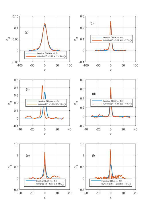
Figure 7: The solitary density profile with, (a) $\kappa$ = 0.5, (b) $\kappa$ = 1.0, (c) $\kappa$ = 1.5, (d) $\kappa$ = 2.0, (e) $\kappa$ = 2.5, (f) $\kappa$ = 2.7, in both the numerical and analytical limit of the QLCA theory, for $h_{1}$ = 4, $h_{2}$ = 3.9, $U_{0}$ =0.1

Remarkably, this initial transient is not produced in preseudospectral numerical evolution in the low $\kappa$, or weak screening, regime and the initial profiles prescribed by the analytical KdV solutions propagate without any significant distortion, indicating that both analytical QLCA and the GH model make a reasonably good prediction of the nonlinear coherent structures, remaining in agreement with the general numerical implementation.

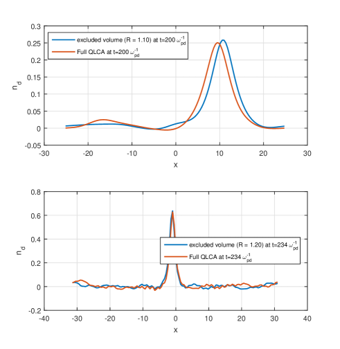
Figure 8: The solitary density profile with, (a) Excluded volume (R) = 1.10, (b) Excluded volume R = 1.20, in both the Excluded volume approximation and Full QLCA $D_{L}$ matrix, for $h_{1}$ = 4, $h_{2}$ = 3.9, $U_{0}$ = 0.1.

Additionally, the numerical approaches using $D_{L}$ based on (6) and (7) were also compared and found to be nearly in agreement with each other. The red and blue curve, in Fig. 8 (a), correspond to the solition structure obtained from the full QLCA $D_{L}$ matrix with $\kappa$ = 1.0 and excluded volume approximation with R = 1.10, respectively. There is no significance difference observed to be developed, accordingly, in the solition structure. Similar behavior of the solition structures can also been seen from Fig. 8(b) at relative higher screening parameter value $\kappa$ = 2.0 in which the solition structures obtained from both the full QLCA $D_{L}$ matrix with $\kappa$ = 2.0 and Excluded volume approximation with R = 1.20, respectively, almost overlap.

The agreement between GH model solutions with the numerical computations in smaller $\kappa$ regime relates, more quantitatively, to the characteristics of linear modes for lower and higher $k$ values, which is analyzed over a range of $\kappa$ values, for example in Fig. 5. Only a moderate variation of $g(k)$ with $\kappa$ for lower $k$ means that $D(k\rightarrow 0)$ can still be derived from the system correlation energy and its derivatives. No analytical approximation is however possible for relatively higher values of $k$ and $\kappa$, and $D_{L}$ remains no longer correctly expressible in terms of the system correlation energy. On the other hand, the general adoptations of $D_{L}$, either (6) or (7), by means of our pseudospectral (spatiotemporal, yet fully resolved in the $k$ values of modes constituting the nonlinear structures) numerical model, accounting for the structural effects continues to describe the smaller wavelengths and relative stronger screened excitations in this limit. Therefore, Numerical simulation accounting for the full structural effects can suitably describe the higher wavelengths and relative stronger screened excitations in such systems.

IV Characterization of analytical nonlinear solitary solutions in weak screening limit

In order to analyze solitary waves in a strongly coupled but weakly screened dusty plasma with finite localization in rather detail, we begin by presenting the amplitude $\phi_{m}$ and width $\Delta$ of the soliton given by Eq. (32) (besides normalized velocity of the $U_{0}$). The amplitude $\phi_{m}$ and width $\Delta$ depend on $\alpha$ and, in turn, on $\kappa$ and $\Gamma$ through factors $A$ and $B$ given by Eq. (29) and (30), respectively. The negative solitary potential profile is plotted in Fig. 6 in the strong coupling (QLCA) limit with different values of screening parameter $\kappa$. For the constant value of $U_{0}$,

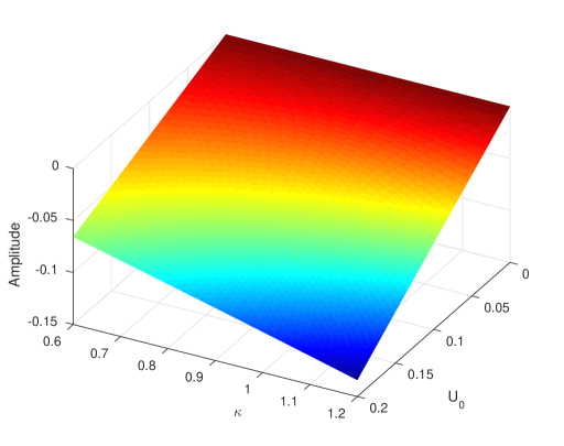
Figure 9: The variation of the amplitude of the negative solitary potential with parameters $\kappa$ and $U_{0}$ for constant value of $h_{1}$ = 4, $h_{2}$ = 3.9 .

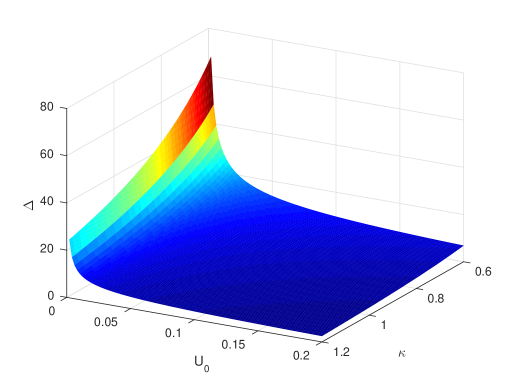
Figure 10: The variation of the width of the negative solitary potential with parameters $\kappa$ and $U_{0}$ for constant value of $h_{1}$ = 4, $h_{2}$ = 3.9.

the amplitude of the solitary wave increases with $\kappa$ in strongly coupled (QLCA) limit since the amplitude has a inverse dependence on with factor $A$ reduces with $\kappa$ in this limit. The width being directly proportional to factor $B$ reduces with $\kappa$ in the strongly coupled (QLCA) limit. This behavior of solitary waves explored for the strongly coupled and localized phase of the dust (adopting QLCA based approach) is in contrast to the effects of strong coupling on a dust solitary wave analyzed in a model where strong-coupling effects are introduced via an effective temperature $T^{\rm(eff)}$ Cousens et al. (2012). A better agreement the soliton solutions recovered in the present treatment is however seen with the Molecular Dynamical (MD) simulation results (Tiwari et al., 2015; Kumar et al., 2017). Moreover, the behavior of solitary waves explored by adopting QLCA based approach is also in contrast to the effects of dust temperature on a dust solitary wave analyzed from the theoretical models (Mamun and Shukla, 2002, 2005) in which the amplitude and width of dust acoustic solitary waves decreases and increases, respectively, with increasing the dust temperature.

The 2D surface plot of the amplitude $\phi_{m}$ and width $\Delta$ of the dust solitary waves are presented in Fig. 9 and 10, respectively, describing their variation with respect to variation of the parameters $U_{0}$ and $\alpha$. For a fix value of $\alpha$, while the amplitude of the dust solitary wave increases with $U_{0}$ its width is shown to decrease, which is a behavior consistent with the well known characteristics of the solitons where the product $|\phi_{m}|\Delta^{2}$ is independent of $U_{0}$.

V Simulations with initial profiles of general form

For simulating more general but initially localized nonlinear perturbations, we have also launched a more general, Gaussian-shaped, initial density perturbations in the pseudospectral simulation procedure given by,

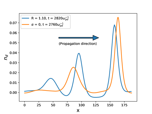
Figure 11: Time evolution profile of an initial Gaussian dust density perturbation in the both weak and strong coupling limit for $\kappa$ = 1.0, $n_{0}$ = 0.05 and $\Delta$ = 20.

$$n_{d}=n_{0}\exp\left[-\left(\frac{x-x_{0}}{\Delta}\right)^{2}\right],$$ (37)

Fig. 11 presents the evolution of the initial Gaussian density perturbation, with $n_{0}$ = 0.05, $\Delta$ = 20 and $x_{0}$ = 64, in both strong ($\alpha\neq 0$, $R=1.1$) and weak ($\alpha=0$) coupling limit of the model, It is evident from the presented evolution that in the weakly coupled limit the perturbation decays into two unequal solitons, whereas it splits in to three unequal amplitude soliton structures when the dust-dust correlations are accommodated in the model with complete localization effects. It can be seen that the taller soliton propagates with a velocity faster than the smaller soliton which remains a well know property of the soliton/solitary wave structures of KdV type.

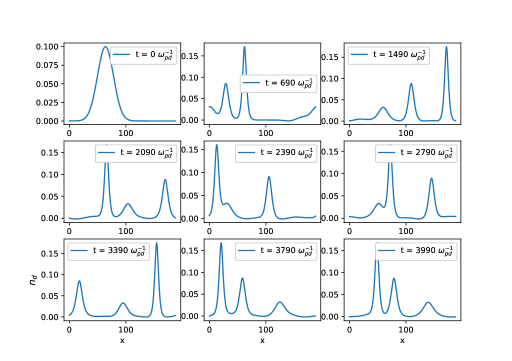
Figure 12: Time evolution of an initial Gaussian dust density perturbation profile in a weakly coupled limit for $\kappa$ = 1.0, $n_{0}$ = 0.1 and $\Delta$ = 20.

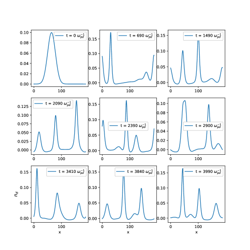
Figure 13: Time evolution of an initial Gaussian dust density perturbation profile in the strongly coupled limit for $\kappa$ = 1.0, R($\kappa$) = 1.10, $n_{0}$ = 0.1 and $\Delta$ = 20.

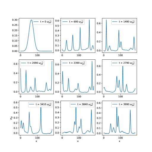
Figure 14: Time evolution of an initial Gaussian dust density perturbation profile in the strongly coupled limit for $\kappa$ = 1.0, R($\kappa$) = 1.10, $n_{0}$ = 0.3 and $\Delta$ = 20.

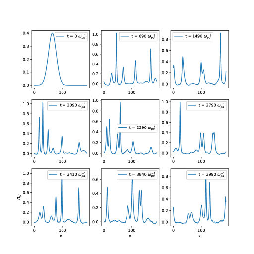
Figure 15: Time evolution of an initial Gaussian dust density perturbation profile in the strongly coupled limit for $\kappa$ = 1.0, R($\kappa$) = 1.10, $n_{0}$ = 0.4 and $\Delta$ = 20.

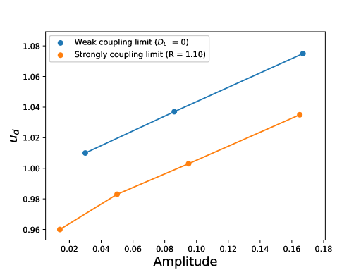
Figure 16: Mach Number ($u_{d}$) of the dust acoustic solitons as a function of their amplitude in the weak and strongly coupling limit for $\kappa$ = 1.0 and $n_{0}$ = 0.1.

A number of more general initial condition structures with a range of initial amplitude are studies further in order to understand the influence, on these excitations, of various initial density perturbation profiles. Fig. 12 presents the evolution of a density perturbation with a relatively higher initial amplitude $n_{0}$ = 0.1 within the weak-coupling limit ($\alpha=0$). The emergence of three unequal height soliton has once again been noted in this case which appears identical to the strong-coupling case presented in Fig. 11. It can therefore be concluded that the effect of strong-coupling is somewhat equivalent to the choice of an increased initial amplitude of the perturbation. The next Fig. 13 presents the evolution of the density perturbation with the initial amplitude $n_{0}=0.1$ however this time in the strong-coupling limit. What is noted is the emergence of a train of four solitons of orderly reducing heights, confirming the equivalence of strong-coupling to the initial amplitude of the perturbation. Since these solitary structures visibly preserve their identities for a considerably longer time (i.e., several orders of inverse dust acoustic frequency) and even after undergoing mutual interaction (or collisions), they indeed represent the dust acoustic soliton structures. Fig. 14 and 15 demonstrate the reasonably consistent solitary evolution of the initial density perturbation with even higher amplitudes, $n_{0}=0.3$ and $n_{0}=0.4$, respectively, up to a sufficiently longer evolution time $\omega_{pd}t=3900$.

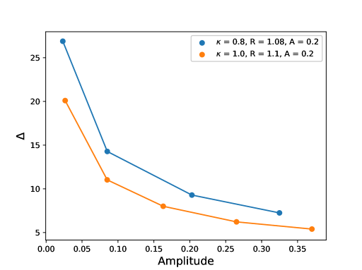
Figure 17: Width ($\Delta$) of the dust acoustic solitons as a function of their amplitude in the strong coupling limit for different value of parameter R($\kappa$).

In order to make a comparison with the theoretical estimates presented in Sec. II, the normalized velocity (to linear dust acoustic velocity) and width of the dust acoustic solitons are presented in Figs. 16 and 17, respectively. These are measured for different excitation amplitudes after the individual solitons appear in both weak and the strong coupling cases. The Mach number $u_{d}$ of the solitary wave increases linearly with amplitude in both strong and weakly coupled limit consistent with the experimental observationsSharma et al. (2014); Nosenko et al. (2002); Bandyopadhyay et al. (2008). The measured Mach number $u_{d}$ of the solitons in the strong-coupling is smaller than in the weak coupling ($\alpha$ = 0) limit of the model. The effect of the strong dust-dust correlation in reducing the phase velocity of the solitons, is consistent with the theoretical predictions of Sec. II. For a fixed value of $R(\Gamma$,$\kappa)$ (the excluded volume parameter) the width of a soliton decreases with increasing the amplitude, as can be seen from Fig. 17. On the other hand, for a fixed value of the soliton amplitude, the width of a soliton decreases with increasing the dust-dust correlation via parameter $\kappa$ or $R(\Gamma$,$\kappa)$. This effect of the dust-dust correlation is also in correspondence with the above theoretical prediction of Sec. II.

Amplitude(A)	Widht($\Delta$)	(A$\Delta^{2}$)
0.0235	26.90	17.040
0.0851	14.28	17.350
0.2029	9.292	17.518
0.3248	7.251	17.077

Table 1: The soliton characteristic property for the parameters $\kappa$ = 0.8, R($\kappa$) = 1.08 and A = 0.2.

Finally, in order to present a more quantitative aspect of the presented numerical soliton solutions we conclude by presenting another well known property of the Kdv solitons, namely, the product of amplitude and squared width, $\phi_{m}\Delta^{2}$, of the solitons which remains independent to the dust acoustic soliton mach number. Our solutions confirm that this property of the dust acoustic soliton is preserved and persists even in the realm of the QLCA approach applied to the soliton formulation, as presented in the form of data in Table 1.

VI Summary and conclusions

To summarize, the nonlinear approach is made to finite amplitude excitations of strongly-coupled fluids such that dust localization effects are present and can not be neglected especially while treating strong screening of localized charges generated by the background plasma, for example in a laboratory dusty plasma. The nonlinear excitations treated under analytical approximations that exclude localization nevertheless prescribe localized solutions with very limited reproducibility by a numerical implementation of more full nonlinear model accounting for the localization by means of the dynamical matrix $D_{L}$ under the quasi-localized charge approximation. Inclusion of the finite dust localization, essentially requiring to account for the structured pair-correlation function $g(r)$, is suitably facilitated by the quasi-localized charge approximation framework. With its present applications remaining limited to spectral domain and hence largely to exploring the linear dispersions, the persisting challenge of inclusion of these effects in a full nonlinear and therefore spatiotemporal formulation is addressed in the present study. This is done by developing and solving an analytical nonlinear model for the localized-phase of a strongly coupled dusty plasma system while incorporating the elements of detailed QLCA formulation. The nonlinear solutions are obtained both by analytical and numerical implementations, in a nonlinear pseudspectral approach, of the dynamical matrix $D_{L}$ duly accounting for a structured pair-correlation function $g(r)$. The characterization of both periodic and coherent solitary nonlinear structures has allowed to identify, in strong screening limit, the contribution over a considerable spectral range spectral which is adequately accounted for by a more general QLCA implementation of the localization by means of nonlinear pseudospectral procedure.

Among main results, we have first shown that an analytical approximation of the QLCA dynamic matrix $D_{L}$(Golden and Kalman, 2000; Rosenberg and Kalman, 1997) in terms of excess energy (the OCP implementation), limited to weak screening limit, reproduces results available from the GH prescription. However, application of the QLCA formulation in its full capacity to the strong screening limit subsequently allows recovery of a strong departure in the evolution of the nonlinear excitations from that of their weak screening counterparts, accessed by OCP limit implementation of the procedure well within QLCA framework. Accordingly, the nonlinear pseudospectral procedure initialized with the analytical coherent solitary solutions of the KdV equation although propagate unmodified in the small $\kappa$ limit, they undergo an initial transient and self-consistently settle down to newer more steeper profiles for large $\kappa$ values. At relatively higher $\kappa$ values the numerical solutions tend to grow extremely steep and acquire cusp-like spatial profiles showing weaker temporal coherence indicating that they are rather governed by a modified KdV equation, as supported by certain recent arguments(Hunter and Saxton, 1991; Kumar Tiwari et al., 2012). The observations that the accessibility to their evolution with enough accuracy is only limited by the numerical resolution of the computations indicate potential applicability of the analysis procedure to rather yet unexplored limits of the parameter space.

In terms of linear structures, the access to larger frequency, or shorter wavelength limit, where the OCP based descriptions, including the original GH dispersion as well as its QLCA counterpart, show strong limitation is now available by means of the presented excluded volume approximation of the QLCA dynamical matrix. The corresponding QLCA linear dispersion is shown to closly agree with the results of the MD simulation in this regime. In essential quantitative terms, the $\kappa\sim 1$ limit for the existing Yukawa fluid models of both periodic linear and coherent nonlinear excitations to show agreement with the experiment and simulations has been overcome by the present QLCA prescription and agreement is now recoverable up to $\kappa\sim 2.7$.

Among its major limitations, the QLCA approach remains unsuitable to an arbitrarily large $\kappa$. It also loses its applicability when approaching the hard sphere interaction limit (Khrapak et al., 2017). The nonlinear processes involving unstable density fluctuations of shorter wavelength, for example, DAW suffer a modulational instability at short wavelengths, can however be captured by the QLCA model and a related nonlinear analysis is being communicated by the authors separately, which also forms a suitable future work to the present study.

VII ACKNOWLEDGMENT

The simulation work presented here is performed on ANTYA cluster at the Institute for Plasma Research (IPR), Gandhinagar, India.

*

Appendix A Incorporation of the strong coupling effects without localization

A.1 Effective strong coupling in random phase limit

While explicit representation of strong coupling by retaining the correlation via dynamical matrix $D_{L,T}$ is central to QLCA approach, a strongly coupled yet random phased state ($g(r)\rightarrow 1$) is treatable by an effective representation of the dust-dust correlation by supplementing the kinetic dust pressure, $P_{dk}$, by an effective pressure, $P_{di}$, or an isothermal dust compressibility  Cousens et al. (2012),

$$\begin{split}\frac{\partial{u}_{{\rm d}x}}{\partial t}+({\bf u}_{{\rm d}}\cdot\nabla){u}_{{\rm d}x}=\frac{q_{\rm d}}{m_{\rm d}}{E}_{x}-\frac{1}{m_{d}n_{d}}\left[\frac{\partial P_{dk}}{\partial x}+\frac{\partial P_{di}}{\partial x}\right].\\ \end{split}$$ (38)

An effective temperature $T_{d}^{\rm(eff)}$, apart from dust kinetic temperature is then used to express the copressibility arising from the correlations,

$$\begin{split}\frac{\partial{u}_{{\rm d}x}}{\partial t}=\frac{q_{\rm d}}{m_{\rm d}}{E}_{x}-\frac{T_{d}^{\rm(eff)}}{m_{d}n_{d}}\frac{\partial n_{d}}{\partial x},\\ \end{split}$$ (39)

where,

$$T_{d}^{\rm(eff)}=\frac{N_{nn}}{3}\Gamma T_{d}(1+\kappa)\exp(-\kappa),$$ (40)

which is a few orders of magnitude higher than the kinetic temperature of the dust.

Eq. (LABEL:momentum-balance-rpa-sc) along with the continuity and Poisson equations produces the linear dispersion relation of the strongly coupled dusty plasma in the random phase limit,

$$\omega^{2}=\left(\frac{d_{1}k^{2}\omega^{2}_{\rm pd}}{1+{k^{2}}}\right)+\beta k^{2},$$ (41)

where $\beta$ and $d_{1}$ are the model parameters defined by the dust and background plasma Cousens et al. (2012).

A.2 Thermodynamic approach to the strong-coupling in random phase limit

One of the simplest approachs to account for the strong coupling effects in this limit has been presented by Khrapak Khrapak and Thomas (2015) in which strong coupling effects are included in the conventional fluid model by supplementing it with the appropriate thermodynamic functions,

$$c^{2}_{s}=\frac{\omega^{2}}{k^{2}}=\omega^{2}_{pd}\left(\frac{1}{\kappa^{2}}+\frac{\gamma\mu}{3\Gamma}\right),$$ (42)

where $\gamma$ and $\mu$ is the adiabatic index and isothermal compresssibility modulus, respectively. To evaluate the effects of strong coupling on the dispersion relation and sound velocity of Yukawa fluid, the parameter $\gamma$ and $\mu$ are represented in term of thermodynamic functions of Yukawa fluid as,

$$\gamma\mu=\mu+\frac{\left[p-\Gamma(\partial p/\partial\Gamma)\right]^{2}}{u-\Gamma(\partial p/\partial\Gamma)},$$ (43)

where u, p and $\mu$ are the internal energy, pressure and isothermal compresssibility modulus, respectively, which account for the both particle-particle correlation and plasma-related effects (Khrapak, 2015). These linear dispersion are compared with the more general linear dispersion generated by QLCA of linear perturbation equation (II), obtained as below. With the isothermal compressiblity having negative sign, at sufficiently strong coupling this results in the loss of solution at large $k$ values, leading to null frequency observed in dispersion relation plotted with a green line in Fig. 1. This issue is effectively resolved by inclusion of localization in QLCA model as discussed further below.

A.3 Generalized hydrodynamic model (GH)

The GH model, based on phenomenological dispersion (Kaw, 2001), incorporates the strongly coupling effects via nonlocal visco-elasticity with memory effects arising from the strong correlation among constituent particles. In a long wavelength limit, the dispersion relation of strongly coupled yukawa system in their kinetic regime can be written as,

$$\omega^{2}(k)=\frac{\omega^{2}_{\rm pd}k^{\rm 2}}{k^{\rm 2}+\kappa^{\rm 2}}+\frac{\omega^{2}_{\rm pd}k^{2}}{\Gamma}\left(\frac{1}{3}+\frac{4}{45}u_{ex}\right),$$ (44)

where $u_{ex}$ is the normalized excess energy given in Ref. (Kaw, 2001).

References

- Peng et al. (2007) F. Peng, E. F. Brown, and J. W. Truran, The Astrophysical Journal 654, 1022 (2007).
- Dantan et al. (2010) A. Dantan, J. Marler, M. Albert, D. Guénot, and M. Drewsen, Physical review letters 105, 103001 (2010).
- Killian et al. (2007) T. C. Killian, T. Pattard, T. Pohl, and J. Rost, Physics reports 449, 77 (2007).
- Wang et al. (2001) X. Wang, A. Bhattacharjee, and S. Hu, Phys. Rev. Lett. 86, 2569 (2001).
- Hou et al. (2004) L.-J. Hou, Y.-N. Wang, and Z. Mišković, Physical Review E 70, 056406 (2004).
- Hou et al. (2009) L.-J. Hou, Z. Mišković, A. Piel, and M. S. Murillo, Physical Review E 79, 046412 (2009).
- Kaw and Sen (1998) P. Kaw and A. Sen, Physics of Plasmas 5, 3552 (1998).
- Kaw (2001) P. Kaw, Physics of Plasmas 8, 1870 (2001).
- Golden and Kalman (2000) K. I. Golden and G. J. Kalman, Physics of Plasmas 7, 14 (2000).
- Donko et al. (2008) Z. Donko, G. J. Kalman, and P. Hartmann, Journal of Physics: Condensed Matter 20, 413101 (2008).
- Kalman et al. (2005) G. J. Kalman, K. I. Golden, Z. Donko, and P. Hartmann, Journal of Physics: Conference Series 11, 254 (2005).
- Golden et al. (2009) K. I. Golden, G. J. Kalman, Z. Donko, and P. Hartmann, Journal of Physics A: Mathematical and Theoretical 42, 214017 (2009).
- Lee and Kalman (2011) C.-J. Lee and G. J. Kalman, Journal of the Korean Physical Society 58, 448 (2011).
- Morfill and Ivlev (2009) G. E. Morfill and A. V. Ivlev, Reviews of modern physics 81, 1353 (2009).
- Khrapak and Thomas (2015) S. A. Khrapak and H. M. Thomas, Physical Review E 91, 033110 (2015).
- Yaroshenko et al. (2010) V. Yaroshenko, V. Nosenko, and G. Morfill, Physics of Plasmas 17, 103709 (2010).
- Khrapak et al. (2016) S. A. Khrapak, B. Klumov, L. Couedel, and H. M. Thomas, Physics of Plasmas 23, 023702 (2016).
- Kalman et al. (2000) G. Kalman, M. Rosenberg, and H. DeWitt, Physical review letters 84, 6030 (2000).
- Ohta and Hamaguchi (2000) H. Ohta and S. Hamaguchi, Physical Review Letters 84, 6026 (2000).
- Nunomura et al. (2005) S. Nunomura, S. Zhdanov, D. Samsonov, and G. Morfill, Physical review letters 94, 045001 (2005).
- Yang et al. (2017) C. Yang, M. Dove, V. Brazhkin, and K. Trachenko, Physical review letters 118, 215502 (2017).
- Sharma et al. (2014) S. Sharma, A. Boruah, and H. Bailung, Physical Review E 89, 013110 (2014).
- Boruah et al. (2016) A. Boruah, S. Sharma, Y. Nakamura, and H. Bailung, Physics of Plasmas 23, 093704 (2016).
- Rosenberg and Kalman (1997) M. Rosenberg and G. Kalman, Physical Review E 56, 7166 (1997).
- Kumar and Sharma (2021) P. Kumar and D. Sharma, Physics of Plasmas 28, 083704 (2021).
- Fornberg (1998) B. Fornberg, A practical guide to pseudospectral methods, 1 (Cambridge university press, 1998).
- Donkó et al. (2003) Z. Donkó, P. Hartmann, and G. Kalman, Physics of Plasmas 10, 1563 (2003).
- Khrapak (2017) S. A. Khrapak, AIP Advances 7, 125026 (2017).
- Bandyopadhyay et al. (2007) P. Bandyopadhyay, G. Prasad, A. Sen, and P. Kaw, Physics Letters A 368, 491 (2007).
- Mokshin et al. (2022) A. V. Mokshin, I. I. Fairushin, and I. M. Tkachenko, Physical Review E 105, 025204 (2022).
- Zhdanov et al. (2003) S. Zhdanov, S. Nunomura, D. Samsonov, and G. Morfill, Physical Review E 68, 035401 (2003).
- Wong et al. (2017) C.-S. Wong, J. Goree, and Z. Haralson, IEEE Transactions on Plasma Science 46, 763 (2017).
- Davidson (2012) R. Davidson, Methods in nonlinear plasma theory (Elsevier, 2012).
- Shukla and Mamun (2015) P. K. Shukla and A. Mamun, Introduction to dusty plasma physics (CRC press, 2015).
- Coutsias et al. (1989) E. Coutsias, F. Hansen, T. Huld, G. Knorr, and J.-P. Lynov, Physica Scripta 40, 270 (1989).
- Cousens et al. (2012) S. E. Cousens, S. Sultana, I. Kourakis, V. V. Yaroshenko, F. Verheest, and M. A. Hellberg, Physical Review E 86, 066404 (2012).
- Tiwari et al. (2015) S. K. Tiwari, A. Das, A. Sen, and P. Kaw, Physics of Plasmas 22, 033706 (2015).
- Kumar et al. (2017) S. Kumar, S. K. Tiwari, and A. Das, Physics of Plasmas 24, 033711 (2017).
- Mamun and Shukla (2002) A. Mamun and P. Shukla, Physica Scripta 2002, 107 (2002).
- Mamun and Shukla (2005) A. Mamun and P. Shukla, Plasma physics and controlled fusion 47, A1 (2005).
- Nosenko et al. (2002) V. Nosenko, S. Nunomura, and J. Goree, Physical review letters 88, 215002 (2002).
- Bandyopadhyay et al. (2008) P. Bandyopadhyay, G. Prasad, A. Sen, and P. Kaw, Physical review letters 101, 065006 (2008).
- Hunter and Saxton (1991) J. K. Hunter and R. Saxton, SIAM Journal on Applied Mathematics 51, 1498 (1991).
- Kumar Tiwari et al. (2012) S. Kumar Tiwari, A. Das, P. Kaw, and A. Sen, Physics of Plasmas 19, 013706 (2012).
- Khrapak et al. (2017) S. Khrapak, B. Klumov, and L. Couëdel, Scientific Reports 7, 1 (2017).
- Khrapak (2015) S. A. Khrapak, Plasma Physics and Controlled Fusion 58, 014022 (2015).