Confidence-driven Bounding Box Localization for Small Object Detection

Abstract

Despite advancements in generic object detection, there remains a performance gap in detecting small objects compared to normal-scale objects. We for the first time observe that existing bounding box regression methods tend to produce distorted gradients for small objects and result in less accurate localization. To address this issue, we present a novel Confidence-driven Bounding Box Localization (C-BBL) method to rectify the gradients. C-BBL quantizes continuous labels into grids and formulates two-hot ground truth labels. In prediction, the bounding box head generates a confidence distribution over the grids. Unlike the bounding box regression paradigms in conventional detectors, we introduce a classification-based localization objective through cross entropy between ground truth and predicted confidence distribution, generating confidence-driven gradients. Additionally, C-BBL describes a uncertainty loss based on distribution entropy in labels and predictions to further reduce the uncertainty in small object localization. The method is evaluated on multiple detectors using three object detection benchmarks and consistently improves baseline detectors, achieving state-of-the-art performance. We also demonstrate the generalizability of C-BBL to different label systems and effectiveness for high-resolution detection, which validates its prospect as a general solution.

1 Introduction

Nowadays, the object detection task [5, 15] has been greatly promoted due to advances in deep convolutional neural networks (DNNs) [8]. Despite the progress, small object detection remains a challenging problem. For instance, Cascade R-CNN [2] achieves 55.8 and 66.7 mAP on medium and large objects but only obtains 35.5 mAP on small objects, i.e., defined as objects with scales less than 32 $\times$ 32 pixels, on the COCO [15] dataset. This significant performance gap between small and normal-sized objects presents a hindrance to the implementation of object detectors in various real-world scenarios.

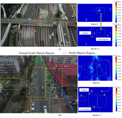
Figure 1: Normalized gradient maps of Faster-RCNN backbone trained with 1$\times$ schedule. The top and bottom maps indicate epoch 0 and epoch 12, respectively. In (a) and (b), normal-scale objects converge in epoch 12 while small objects’ gradients remain salient.

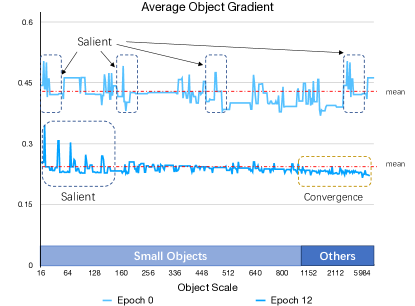
Figure 2: Average object gradient on the saliency maps generated by 50 randomly selected pictures in the VisDrone dataset[28]. The top and bottom curve indicates epoch 0 and epoch 12, together illustrate that normal-scale objects converge in epoch 12 while small objects’ gradients remain salient.

Existing methods for small object detection mainly focus on feature enhancement to improve detection accuracy. As small objects have limited pixel inputs, they are susceptible to insufficient feature representation, particularly in deeper network layers. As a consequence, small objects tends to generate noisy and uncertain predictions, which can also detrimental to small objects as they are more sensitive to offset shifts and even minor perturbations can significantly decrease Intersection over Union (IoU). Recent methods, such as [3, 13, 1, 25], have attempted to address this issue by increasing the resolution of feature maps using the Feature Pyramid Network (FPN) or by slicing high-resolution inputs into patches for improved inference and fine-tuning. To reduce the computation cost, cascaded sparse queries are employed to process high-resolution feature maps while maintaining detection accuracy.

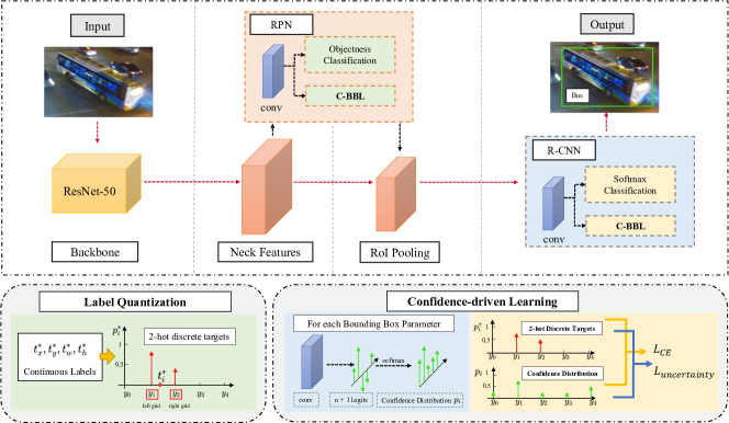
Figure 3: Pipeline of C-BBL with the Faster R-CNN framework.

However, we demonstrate that conventional object regression can cause significant gradient distortion on small objects and thus cause a larger uncertainty for localization, which is overlooked in existing methods [10, 19, 27]. We present the saliency maps generated by Faster R-CNN with a ResNet-18 backbone on the VisDrone dataset[28] in Fig. 1 and the statistical analysis of the average object gradient in Fig. 2. The visualization indicates that the detector is well-converged only for normal-scale objects (yellow area in Fig. 1), while last-epoch gradients remain salient in small object areas (red area in Fig.,1), degrading the detector’s performance on small objects.

We propose a novel Confidence-driven Bounding Box Localization (C-BBL) method to address the issue of localization gradient distortion. Unlike conventional prevailing bounding box regression strategies, we introduce a classification-based localization objective function to generate confidence-driven gradients with a new perspective of reducing uncertainty on localization. The framework of our C-BBL is outlined in Fig. 3. C-BBL first quantizes continuous labels into grids and formulates two-hot ground truth labels. During prediction, the bounding box head generates a confidence distribution over the grids, which can be used to estimate the object location based on its expectation. By utilizing the cross entropy between ground truth and predicted confidence distribution as the objective, our method produces stable and confidence-driven gradients. Furthermore, we design a uncertainty loss based on the entropy in the labels and predictions to further reduce uncertainty in small object prediction. Combining these strategies, our method facilitates a faster training convergence and accurate small object localization. To summarize, our main contributions are three-fold:

1. We propose a novel confidence-driven bounding box localization (C-BBL) method to alleviate gradient distortion problem among small objects.

2. We quantize the continuous labels into interval non-uniform two-hot labels and introduce a confidence-driven objective function to calculate more stable gradients, achieving better convergence for small object detection.

3. Our C-BBL demonstrates superiority over baseline detectors, and achieve state-of-the-art performance with a small-object-oriented detector, validating its prospect as a general solution for the object detection task.

2 Related Work

Object Detection and Localization. Deep Learning based object detectors can be generally classified into two categories: two-stage and single-stage object detectors. Two-stage detectors, such as Faster R-CNN [19], RPN [13], and Cascade R-CNN [2], first generate region proposals and then refine them in a second stage. On the other hand, single-stage detectors, such as RetinaNet [14] and YOLO [18], concurrently classify and regress objects, making them highly efficient, but lower in accuracy. In the object localization branch, R-CNN [7] utilizes the L2 norm between predicted and target offsets as the objective function, which may cause gradient explosions when errors are significant. To address this issue, Fast R-CNN [6] and Faster R-CNN [19] introduced the Smooth L1 loss, which maintains consistent gradients even for large prediction errors. Recent methods, including UnitBox [26], Generalized IoU Loss (GIoU)[20], and Complete IoU Loss (CIoU)[27], aim to improve localization accuracy by utilizing IoU-related (Intersection over Union) values as regression targets. IoU Loss [26] utilized the negative log of IoU as objective functions directly, which incorporates the dependency between box coordinates and adapts to multi-scale training. The GIoU [20] loss extends the IoU Loss to non-overlapping cases by considering the shape properties of the compared objects. CIoU Loss [27] incorporates additional geometric measurements, such as overlap area, central point distance, and aspect ratio, leading to improved convergence.

Small Object Detection. Small object detection, together with recognition and segmentation, is a challenging computer vision task due to the natural bound of pixel input. Challenges in small object detection can be summarized as follows: insufficient feature representation, feature vanish after down-sampling [11], and fewer positive samples assigned due to their sensitivity in IoU (intersection over union) calculation [24]. Works have been proposed to tackle the problems, which can be classified into four categories: features enhancement [3, 13, 4]; data augmentation and oversampling [30, 16]; scale-aware training [12, 22]; reducing IoU sensitivity [24, 23].

Our method is orthogonal to existing detectors from a new perspective of solving the gradient distortion problem for small object localization. To this end, we introduce a classification-based localization objective that generates confidence-driven gradients. C-BBL also introduces a uncertainty loss based on distribution entropy in labels and predictions to reduce uncertainty in small object prediction.

3 Method

Most object detection regression methods utilize the distance between prediction and target box as the object function. However, this approach can generate distorted gradients for small objects and lead to less accurate localization. In this section, we first analyze the gradient distortion problem in norm-based and IoU-based regression methods, then introduces the confidence-driven bounding box localization (C-BBL) method as a solution.

3.1 Preliminaries

We denote $T_{x},T_{y},T_{w},T_{h}$ and $\hat{T}_{x},\hat{T}_{y},\hat{T}_{w},\hat{T}_{h}$ as the predicted offsets from assigned anchors the target offsets respectively, where $(x,y,w,h)$ are the center coordinates, width and height of a bounding box. Following previous detectors [7, 6, 19], the offsets of four coordinates are formulated as:

$$\small\begin{split}\{T_{x},T_{y},T_{w},T_{h}\}&=\{\frac{x-x_{a}}{w_{a}},\frac{y-y_{a}}{h_{a}},\log\frac{w}{w_{a}},\log\frac{h}{h_{a}}\},\\ \{\hat{T}_{x},\hat{T}_{y},\hat{T}_{w},\hat{T}_{h}\}&=\{\frac{\hat{x}-x_{a}}{w_{a}},\frac{\hat{y}-y_{a}}{h_{a}},\log\frac{\hat{w}}{w_{a}},\log\frac{\hat{h}}{h_{a}}\},\end{split}$$ (1)

where $(x,y,w,h),(\hat{x},\hat{y},\hat{w},\hat{y})$ and $(x_{a},y_{a},w_{a},h_{a})$ are generated from the predicted box, ground-truth box and the candidate box, respectively.

3.2 Gradient Distortion in Small Objects

Norm-based Regression. Take $\mathcal{L}_{2}$ loss as an example:

$$\small\begin{split}\mathcal{L}_{2}(T_{x},\hat{T}_{x})=\|T_{x}-\hat{T}_{x}\|_{2}.\end{split}$$ (2)

Note that Eq. 2 is likewise for $y,w,h$. The gradient of offsets is further calculated as:

$$\small\begin{split}\frac{\partial\mathcal{L}_{2}(T_{x},\hat{T}_{x})}{\partial T_{x}}&=2(T_{x}-\hat{T}_{x})=\frac{x-\hat{x}}{w_{a}},\;\;\operatorname{likewise}\operatorname{for}y,\\ \frac{\partial\mathcal{L}_{2}(T_{w},\hat{T}_{w})}{\partial T_{w}}&=2(T_{w}-\hat{T}_{w})=\log w-\log\hat{w},\;\;\operatorname{likewise}\operatorname{for}h.\end{split}$$ (3)

As shown, the gradient of $T_{x}$ and $T_{y}$ are affected by the anchor scales $w_{a}$ and $h_{a}$. Since small objects are assigned with smaller scale anchors, the gradients appear larger even when the absolute prediction gap is the same as that of normal-scale objects, which can lead to uneven learning steps and the gradient distortion phenomenon in the final epochs.

Replacing $\mathcal{L}_{2}$ loss, Fast R-CNN [6] adopts Smooth $\mathcal{L}_{1}$ loss function which is:

$$\small\begin{split}\operatorname{Smooth}\operatorname{-}\mathcal{L}_{1}(T_{x},\hat{T}_{x})=\left\{\begin{matrix}\frac{(T_{x}-\hat{T}_{x})^{2}}{2\beta},&|T_{x}-\hat{T}_{x}|\leq\beta\\ |T_{x}-\hat{T}_{x}|-\frac{\beta}{2},&\operatorname{otherwise}\end{matrix}\right.,\\ \frac{\partial\operatorname{Smooth}\operatorname{-}\mathcal{L}_{1}(T_{x},\hat{T}_{x})}{\partial T_{x}}=\left\{\begin{matrix}\frac{T_{x}-\hat{T}_{x}}{\beta},&|T_{x}-\hat{T}_{x}|\leq\beta\\ {sign}(T_{x}-\hat{T}_{x}),&\operatorname{otherwise},\end{matrix}\right..\end{split}$$ (4)

where $sign(\cdot)$ denotes the symbolic function, and these two equations are likewise for $y,w,h$. The Smooth-$\mathcal{L}1$ loss function exhibits the same distortion when offsets are smaller than the threshold $\beta$. When offsets are larger than $\beta$, gradients are clipped to $sign(T_{x}-\hat{T}_{x})$ to prevent potential numerical instability, but this approach fails to accurately reflect the degree of error. Since small objects hold higher uncertainty in regression, they tend to generate noisy predictions with more significant errors, which cannot be distinguished based on gradient and result in slower convergence.

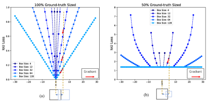
Figure 4: IoU loss on a generic case. (a): prediction is 100% ground-truth sized, (b): prediction is 50% ground-truth sized. The gradient of smaller objects are higher when offset is the same, due to its IoU sensitivity, leading to difficulty distorted gradients. Color indicates different scales of input and ground-truth.

IoU-based Regression. We illustrate gradient distortion in the IoU loss [26] as an example. Let $I$ and $U$ be the insertion and union between the ground truth $(x,y,w,h)$ and predicted box $(\hat{x},\hat{y},\hat{w},\hat{h})$, the IoU loss is calculated as:

$$\mathcal{L}_{\operatorname{IoU}}=-\operatorname{ln}(\frac{I}{U}).$$ (5)

Following [24], we consider a generic scenario where the prediction and the ground truth are square boxes and horizontally aligned. We assume both prediction and the ground truth are the same size in Fig. 4 (a), and prediction is 50% the size of the ground truth in Fig. 4 (b). By shifting their centers with $x$, we observe that smaller objects have higher loss values and steeper gradients (i.e., slope of the loss), leading to distortion in the level of difficulty and more challenging convergence.

3.3 Confidence-driven Bounding Box Localization

To address the gradient distortion problem in small objects, we introduce the Confidence-driven Bounding Box Localization (C-BBL) method, which rectifies the gradients and explores the uncertainty in the regression process. Unlike conventional regression methods that estimate continuous parameters, C-BBL predicts a confidence distribution by discretizing continuous labels into two-hot representations. With a classification-based learning objective, C-BBL generates confidence-driven gradients, resulting in higher localization accuracy for small objects. Additionally, we model the uncertainty in the predicted distribution and minimize it to the lower bound, effectively reducing turbulence in small object predictions. We demonstrate the effectiveness of C-BBL in the Faster R-CNN framework and highlight its generalizability to other label systems.

3.3.1 Label Quantization

Figure 3 illustrates the pipeline of C-BBL. To generate stabler gradient, C-BBL employs a classification-based learning objective and quantizes the labels. Specifically, we first segment the continuous regression range $[-\alpha,\alpha]$ uniformly into $n+1$ grids, resulting in the discrete grid set $Y=\left\{y_{0},y_{1},y_{2},...,y_{n-1},y_{n}\right\}$, with the interval being $\frac{2\alpha}{n+1}$. The representative value of the $i$-th grid can be obtained as follows:

$$y_{i}=-a+i*\frac{2\alpha}{n+1},i\in\left\{0,1,...,n-1,n\right\}.$$ (6)

We cast the continuous ground truth $t^{*}$ to the discrete grid set $Y$ by identifying their left and right grid as $i_{\operatorname{left}}$ and $i_{\operatorname{right}}$:

$$\small\begin{split}y_{i}^{\operatorname{left}}&\leq t^{*}<y_{i}^{\operatorname{right}},\\ y_{i}^{\operatorname{left}}&=-a+i_{\operatorname{left}}*\frac{2\alpha}{n+1},\\ i_{\operatorname{right}}&=i_{\operatorname{left}}+1.\end{split}$$ (7)

The network can learn to localize by predicting the left and right grid. However, the simple quantization fails to retain the precise location within the target interval. To achieve fine-grained quantization, we propose 2-hot discrete targets $p^{*}$ that encode the mid-interval information. Specifically, we calculate the distance between $t^{*}$ to the left and right grid, and then normalize their sum to one, as follows:

$$\small p^{*}_{i}=\left\{\begin{matrix}\frac{n+1}{2\alpha}(y_{i}^{\operatorname{right}}-t^{*}),&i=i_{\operatorname{left}}\\ \\ \frac{n+1}{2\alpha}(t^{*}-y_{i}^{\operatorname{left}}),&i=i_{\operatorname{right}}\\ \\ 0.&\operatorname{otherwise}\end{matrix}\right.$$ (8)

Therefore, the continuous ground truth $t^{*}$ can be fully recovered from discrete target $p^{*}$ by weight averaging the left and right grid as $t^{*}=y_{i}^{\operatorname{left}}*p_{i}^{\operatorname{left}*}+y_{i}^{\operatorname{right}}*p_{i}^{\operatorname{right}*}$.

3.3.2 Interval Non-uniform (IN) Labels

In offset-based label systems, target values decrease with training. As a result, targets are constantly quantized into the same grid interval after some iterations, resulting in ineffective training. To address this issue, we propose interval non-uniform labels that transform the original label representation $y_{i}$ into an exponential form, resulting in interval-increasing grids. The derivation of the interval non-uniform labels is as follows:

$$\small\begin{split}y_{i}^{\prime}=\left\{\begin{matrix}\frac{\alpha}{{e^{\alpha\cdot\beta}-1}}\times(e^{\beta\cdot y_{i}}-1),&y_{i}\geq 0,&\\ \frac{\alpha}{{e^{\alpha*\beta}-1}}\times(1-e^{-\beta\cdot y_{i}}),&y_{i}<0\\ \end{matrix}\right.\\ y_{i}^{\prime}-y_{i-1}^{\prime}=\frac{\alpha}{{e^{\alpha\cdot\beta}-1}}\times(e^{\beta\cdot y_{i+1}}-e^{\beta\cdot y_{i}}).\end{split}$$ (9)

The new label representations $y_{i}^{\prime}$ are symmetrical around zero, ranging from $-\alpha$ to $\alpha$. The length of each interval is controlled by a factor $\beta$, which determines the density of grid points around zero. Higher values of $\beta$ lead to denser grid points. Interval non-uniform labels are well-suited for two-stage and some one-stage detectors, such as the YOLO series, and can be easily integrated into C-BBL training and inference without any additional cost.

3.3.3 Confidence-driven Learning

C-BBL estimates box location by predicting the 2-hot discrete label $p^{*}$. To this end, the bounding box head generates $n+1$ independent logits $l\in R^{n+1}$ for each bounding box parameter. In consistency with the discrete label, we normalize the logits by a softmax layer and obtain the confidence distribution over the grids, where $p_{i}=\frac{exp(l_{i})}{\sum_{i=0}^{n}exp(l_{i})}$.

There are multiple ways to restore the continuous prediction $\hat{t}$ from confidence distribution $p$. An intuitive approach is to select the top-2 scores $p_{1}$ and $p_{2}$ and weight their corresponding grid as $\hat{t}=y_{1}^{\prime}*p_{1}+y_{2}^{\prime}*p_{2}$, which is not numerically stable in the early stages of training when the distribution is flat. Therefore, we utilize the full-band $p$ and calculate the expectation as continuous prediction:

$$\small\hat{t}=\sum_{i=0}^{n}p_{i}*y_{i}^{\prime}.$$ (10)

In optimization, we propose a classification-based learning objective by utilizing the cross entropy between the predicted distribution $p$ and ground truth label $p^{*}$ , illustrated as follows:

$$\small\begin{split}L_{CE}(p,p^{*})&=-\sum_{i=0}^{n}p^{*}_{i}log(p_{i})\\ &=-p^{*}_{i_{left}}log(p_{i_{left}})-p^{*}_{i_{right}}log(p_{i_{right}}).\\ \end{split}$$ (11)

We then demonstrate gradient of the CE Loss is stable and confidence-driven.

$$\frac{\partial L_{CE}(p,p^{*})}{\partial l_{i}} =\frac{\partial L_{CE}(p,p^{*})}{\partial l_{i}}\times\frac{\partial p_{i}}{\partial l_{i}}$$ (12)

$$\;\;\;\;+\sum_{j\neq i}\frac{\partial L_{CE}(p,p^{*})}{\partial p_{j}}\times\frac{\partial p_{j}}{\partial l_{i}}$$

$$=\left\{\begin{matrix}p_{i}-\frac{n+1}{2\alpha}(t_{right}-t^{*}),&i=i_{left}\\ p_{i}-\frac{n+1}{2\alpha}(t^{*}-t_{left}),&i=i_{right}\\ p_{i},&otherwise\end{matrix}\right.$$

$$=p_{i}-p_{i}^{*}.$$

Eq. (12) shows the gradient of CE with respect to logits is the difference between the confidence $p_{i}$ and its ground truth $p^{*}_{i}$. Consequently, the gradient norm of all logits is bounded between zero and one, which is naturally normalized for objects across all scales, resulting in more stable optimization for small objects than L2 and the IoU loss and avoids the distortion problem.

Further, the gradient of CE changes with the confidence difference $p-p^{*}$. Consequently, C-BBL achieves confidence-driven learning, in which bigger confidence difference would enlarge the gradient and descent step, making it easier to escape the sub-optimized locations in the optimization space of the detector.

3.3.4 Uncertainty Minimization

Small objects tends to generate uncertain predictions due to the lack of feature input. To alleviate the issue, we model the uncertainty in the predicted distribution $p$ and minimize it to the lower bound.

$$\begin{split}&L_{\operatorname{uncertainty}}(p,p^{*})=|\mathcal{H}(p^{*})-\mathcal{H}(p)|\\ &=|-\sum_{i=0}^{n}-p^{*}_{i}*log(p^{*}_{i})-\sum_{i=0}^{n}p_{i}*log(p_{i})|.\end{split}$$ (13)

Following Shannon’s information theory [21], C-BBL utilizes entropy to model the uncertainty in $p$. Entropy of $p$ achieves the lowest when some $p_{i}$ is 1, indicating the model is completely sure of the location. Entropy of $p$ achieves the highest when $p$ follows a uniform distribution and all discrete positions are equally alike. In C-BBL, the uncertainty lower bound is the entropy of $p^{*}$ since the discrete targets are two-hot. Consequently, we set up an uncertainty minimization (UM) loss to promote certain and accurate localization, as stated in Eq. (13), which can effectively alleviate the turbulence in small objects prediction.

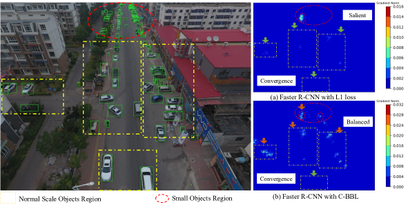
Figure 5: Comparing the normalized gradients of Faster R-CNN backbone in epoch 12. The top contour indicates Faster R-CNN trained with L1 loss and the bottom C-BBL. In (a), normal-scale objects reach convergence while small objects’ gradients remain salient, indicating distortion. In (b), gradients are balanced between normal-scale and small objects while some normal-scale region reach convergence, alleviating the distortion.

4 Experiments

Regression	Stage		mAP	AP50	APs
Loss	RPN	R-CNN
L1	-	-	21.3	36.4	12.8
Smooth-L1	-	-	21.5	36.4	12.7
CE	$\surd$		21.9	37.4	13.2
		$\surd$	22.1	37.1	13.2
	$\surd$	$\surd$	22.1	37.4	13.1
CE + UM	$\surd$	$\surd$	22.7	38.4	13.9
CE + UM + IN Labels	$\surd$	$\surd$	22.9	38.1	14.0

Table 1: Detection performance on the VisDrone validation set with the ResNet-50 Faster R-CNN framework.

In this section, we first provide ablation studies of the C-BBL and compare the method against state-of-the-art object detectors in small object detection. Extensive results reveal that our method outperforms the baselines by a considerable margin and achieve state-of-the-art performance.

4.1 Datasets and Implementation Details

Datasets. We first conduct the ablative study and hyper-parameter selection on drone-shot image specialized VisDrone [28] dataset, in which small objects dominate the scale distribution. We further conduct experiments on the VisDrone [28] dataset, the COCO 2017 [15] object detection track and the PASCAL VOC dataset  [5]. Specifically, we train the models on COCO train2017 and evaluate the models on COCO val2017. For experiments conducted on VOC [5], we use the VOC trainval2012 together with VOC trainval2007 sets to train our model, which contains approximately 16k images, and the VOC test2007 set to evaluate our C-BBL, which contains 4952 images.

Implementation Details. Our C-BBL is trained with the Faster R-CNN [19], Cascade R-CNN [2] and TPH-YOLOv5 [29] framework. For Faster R-CNN [19], we select ResNet-50 and ResNet-101 [9] as backbones. Following default configurations, we adopt 1000$\times$600 as the input resolution on the VOC [5] dataset with total batch size 32, 1333$\times$800 on the VisDrone [28] and COCO [15] dataset with batch size set as 16. For fair comparisons, we utilize default hyper-parameters, 1$\times$ learning schedule (12 epochs) without multi-scale training. We also evaluate C-BBL on a small-object-oriented detector TPH-YOLOv5 [29]. In related experiments, we utilize the default hyper-parameters and weights supplied in  [29] and train 80 epochs. To test the multi-scale functionality, we adopt two sets of input resolution: 640$\times$640 and 1536$\times$1536 on the VisDrone dataset, with the batch size being 16 and 4, respectively. We used PyTorch [17] to implement the C-BBL and ran our experiments on 4 NVIDIA 3090Ti GPUs, each with 24 GB of memory.

Stage	range	grid num ($n$)	mAP	AP50	APs
RPN	2	2	21.8	36.9	12.9
		4	21.9	37.1	13.0
		10	21.9	37.4	13.2
		20	21.8	37.1	13.0
R-CNN	5	5	22.1	37.1	13.2
		10	21.9	37.1	13.1
		20	21.7	37.1	13.1
		40	21.8	36.8	12.8

Table 2: The effect of different grid number $n$ in label quantization with Faster R-CNN.

4.2 Ablation Study and Analysis

In the following experiments, we show that C-BBL leads to consistent performance increase when applied on baseline detectors and explore the best-performed structure of C-BBL by ablating and tuning its parts. We set Faster R-CNN with ResNet-50 [9] as the baseline and perform all tests on VisDrone validation.

Label Quantization and Localization Loss. Label quantization allows us to apply the CE and UM loss in C-BBL, which derives confidence-driven learning. According to Tab. 1, the CE loss achieves $22.1$ mAP when applied on both RPN and R-CNN, $+0.9$ mAP compared to L1 loss and $+0.6$ mAP compared to Smooth-L1 loss, converging to better solution than conventional regression methods. UM loss further increase the detection performance to $22.7$ mAP, validating the effectiveness of uncertainty modeling using entropy. We show in Figure. 5 that C-BBL alleviates the gradient distortion problem as gradients of small object become less salient in epoch 12, compared to L1 loss.

C-BBL Structure Analysis. We apply the CE loss to both stages in Faster R-CNN and show stage-wise ablation performance. As shown in Tab. 1, C-BBL brings +0.4% mAP and +0.5% AP_s to the Region Proposal Network (RPN) and +0.6% mAP and +0.4% AP_s to the R-CNN stage and similar results combined, which is set as the default in C-BBL. We investigate the effect of different grid number $n$ in both stags in Tab. 2. Results demonstrate that C-BBL is not sensitive to the choice of discrete grid number $n$ in both stages. The consistent improvement in both stages indicates C-BBL’s generalization ability to both the dense prediction (RPN) and fine-tuning (R-CNN) localization scenario, demonstrating its prospects to various detection frameworks.

Variant	(range, grid num)	mAP	AP50
Top-2	(5, 5)	20.4	36.4
Full band		22.1	37.1
Top-2	(5, 10)	20.3	36.2
Full band		21.9	37.1

Table 3: Comparing label restoration methods of C-BBL on the VisDrone validation set, under the ResNet-50 Faster R-CNN framework.

Interval Non-uniform (IN) Labels and Restoration. As shown in Tab. 1, utilizing interval non-uniform (IN) labels brings the optimal results of C-BBL and enlarge the margin to +1.4% mAP and +1.3% AP_s, which shows that the non-uniform design is essential in label quantization and can further improve the performance compared to uniform quantization. We compare two methods for continuous label restoration: weight averaging the top-2 labels versus using with the full-band expectation under different grid numbers. Displayed in Tab. 3, full-band expectation shows consistent superiority in all configurations, highlighting the importance of numerical stability for small objects, which are sensitive to IoU.

Backbone	Method	Input Resolution	mAP	AP50	AP75	APs	APm	APl
ResNet-50	RetinaNet	(1333, 800)	13.9	27.7	-	-	-	-
	GFocal		19.5	32.2	20.1	11.2	30.0	35.6
	ATSS		19.9	35.9	19.5	11.6	30.8	35.1
	Faster R-CNN		21.5	36.4	22.3	12.7	32.9	38.9
	Faster R-CNN + C-BBL		22.9	38.1	24.3	14.0	34.6	38.1
	Cascade R-CNN		22.4	37.0	23.7	13.1	34.1	41.2
	Cascade R-CNN + C-BBL		23.0	37.6	24.1	13.8	34.8	40.4
ResNet-101	Faster R-CNN	(1333, 800)	21.9	37.3	22.5	12.8	34.0	37.9
	Faster R-CNN + C-BBL		23.3	38.7	24.5	14.0	35.6	39.6
	Cascade R-CNN		23.0	38.2	24.1	13.5	35.0	43.8
	Cascade R-CNN + C-BBL		23.6	38.7	24.6	13.9	36.0	43.7
CSP-D53	YOLOv4-tiny	(640, 640)	11.2	21.9	-	-	-	-
	YOLOv4-s		18.1	33.0	-	-	-	-
	YOLOv5-x		24.7	41.2	-	-	-	-
	TPH-YOLOv5-x		26.5	43.3	-	-	-	-
	TPH-YOLOv5-x + C-BBL		27.1	44.3	-	-	-	-
	TPH-YOLOv5-x	(1536, 1536)	39.2	60.5	-	-	-	-
	TPH-YOLOv5-x + C-BBL		40.1	60.9	-	-	-	-

Table 4: Detection performance on the VisDrone validation set.

4.3 Two-stage Detection

Settings. We evaluate C-BBL in two stage detectors Faster R-CNN [19] and Cascade R-CNN [2] under R-50 and large-scale R-101 backbones, where hyperparameters $\alpha$, $n$ are tuned to optimal as Tab. 2 and $\beta$ defaults to 1. We configure 1$\times$ schedule with 12 epochs training schedules. We utilize the same SGD optimizer with initial learning rate of 2e-2, decayed by 0.1 at epoch 8 and 11(1$\times$ schedule), and weight decay of 1e-4.

Method	Input Resolution	mAP	AP50
TPH-YOLOv5-x	(640, 640)	21.8	37.7
+ C-BBL		22.2	38.1
TPH-YOLOv5-x	(1536, 1536)	30.8	50.4
+ C-BBL		31.6	50.7
TPH-YOLOv5-x	(2016, 2016)	33.4	53.3
+ C-BBL		33.6	53.6

Table 5: C-BBL with TPH-YOLOv5 [29] on the VisDrone [28] test-dev.

Results. As shown in Tab. 4, C-BBL with Faster R-CNN increases the base with consistent margins across all metrics on the VisDrone validation set. The improvement is also consistent across different backbones, with C-BBL promoting Faster R-CNN with R-101 backbone $+1.4\%$ mAP and $+1.2\%$ AP_s, highlighting its compatibility with backbones of varying volumes. C-BBL with Cascade R-CNN exhibits similar benefits, $+0.6\%$ mAP to the R-50 and R-101 backbones respectively, surpassing many conventional detectors under the $1333\times 800$ input.

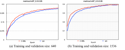
Figure 6: Comparing TPH-YOLOv5 w/o C-BBL under $640^{2}$ and $1536^{2}$ training.

4.4 Label and Resolution Generalization

Settings. To extend our research, we apply C-BBL to TPH-YOLOv5 [29], a proven small-object-oriented detector, by quantizing the YOLO label system and applying the localization losses. In details, regression range $\alpha$ is set to 4 in alignment with the YOLO offset setting, and the grid number defaults to 11. We train the detector under $640^{2}$ and $1536^{2}$ image resolution, where non-uniform label parameter $\beta$ is set to 5 and 3 accordingly. For training, we exclusively used the VisDrone dataset, and evaluated our model on the validation and test-dev datasets.

Label Generalization. Tab. 4 demonstrates C-BBL’s compatibility with the YOLO label system. As shown, C-BBL with TPH-YOLOv5 $+0.6$ and $+0.68$ mAP to the $640^{2}$ and $1536^{2}$ base respectively. C-BBL with TPH-YOLOv5 achieves $40.1$ mAP on the VisDrone validation set without any test-time augmentation, reaching state-of-the-art performance.

Resolution Generalization. C-BBL is generalizable to high-resolution detection inputs, which is the current go-to method in small object detection. On VisDrone validation, C-BBL with TPH-YOLOv5 achieves a $+0.6$ and $+0.68$ mAP improvement on the $640^{2}$ and $1536^{2}$ base, respectively, as shown in Tab. 4. On the test-dev dataset, C-BBL demonstrates consistent improvement, promoting $+0.4$, $+0.8$, and $+0.2$ mAP to the $640^{2}$, $1536^{2}$, and $2016^{2}$ base respectively (see Table 5). We show the mAP curve of $640^{2}$ and $1536^{2}$ training, which demonstrates that C-BBL promotes faster convergence as Fig. 6.

4.5 General Detection

Settings. To demonstrate the merits of C-BBL on general detection benchmark, we evaluate the model on VOC [5] and COCO [15] datasets using a 1$\times$ schedule with 12 epochs of training.

Results. From Tab. 6, C-BBL yields $+1.69\%$ mAP improvement using ResNet 50 and $+0.78\%$ mAP improvement using ResNet 101 over L1 loss on the VOC benchmark. On COCO, C-BBL yields $+0.9\%$ AP_s improvement using ResNet 50 and $+0.8\%$ AP_s improvement using ResNet 101 over the baseline. These results highlight the effectiveness of C-BBL across different network architectures and further emphasize its potential as a versatile and robust solution for various detection tasks.

Back bone	Method	Dataset	mAP	AP50	APs
R50	Faster R-CNN	VOC	78.44	78.40	-
	+ C-BBL		80.13	80.10	-
	Faster R-CNN	COCO	37.4	58.1	21.2
	+ C-BBL		38.0	58.8	22.3
R101	Faster R-CNN	VOC	79.90	80.02	-
	+ C-BBL		80.68	80.70	-
	Faster R-CNN	COCO	39.4	60.1	22.4
	+ C-BBL		40.1	60.7	23.2

Table 6: Experiments with Faster R-CNN on VOC [5] and COCO [15].

5 Conclusions

In this paper, we observe that conventional detectors tend to produce distorted gradients on small objects and introduce a confidence-driven bounding box localization (C-BBL) method to rectify gradients. C-BBL quantizes continuous labels into grids and formulates two-hot ground truth labels. In optimization, C-BBL employs a classification-based learning objective that generates confidence-driven gradient. Further, C-BBL describes a uncertainty loss to reduce the uncertainty in small object prediction. C-BBL exhibits consistent increase on baseline detectors and achieves state-of-the-art performance on a small-object oriented detector, demonstrating the generalizability to different label systems and effectiveness in high-resolution detection, which validates its prospect as a general solution.

References

- [1] Fatih Cagatay Akyon, Sinan Onur Altinuc, and Alptekin Temizel. Slicing aided hyper inference and fine-tuning for small object detection. In 2022 IEEE International Conference on Image Processing (ICIP), pages 966–970. IEEE, 2022.
- [2] Zhaowei Cai and Nuno Vasconcelos. Cascade r-cnn: Delving into high quality object detection. In Proceedings of the IEEE conference on computer vision and pattern recognition, pages 6154–6162, 2018.
- [3] Chenyi Chen, Ming-Yu Liu, Oncel Tuzel, and Jianxiong Xiao. R-cnn for small object detection. In Asian conference on computer vision, pages 214–230. Springer, 2017.
- [4] Liang-Chieh Chen, George Papandreou, Iasonas Kokkinos, Kevin Murphy, and Alan L Yuille. Deeplab: Semantic image segmentation with deep convolutional nets, atrous convolution, and fully connected crfs. IEEE transactions on pattern analysis and machine intelligence, 40(4):834–848, 2017.
- [5] M. Everingham, L. Van Gool, C. K. I. Williams, J. Winn, and A. Zisserman. The pascal visual object classes (voc) challenge. International Journal of Computer Vision, 88(2):303–338, June 2010.
- [6] Ross Girshick. Fast r-cnn. In Proceedings of the IEEE international conference on computer vision, pages 1440–1448, 2015.
- [7] Ross Girshick, Jeff Donahue, Trevor Darrell, and Jitendra Malik. Rich feature hierarchies for accurate object detection and semantic segmentation. In Proceedings of the IEEE conference on computer vision and pattern recognition, pages 580–587, 2014.
- [8] Kaiming He and Jian Sun. Convolutional neural networks at constrained time cost. In Proceedings of the IEEE conference on computer vision and pattern recognition, pages 5353–5360, 2015.
- [9] Kaiming He, Xiangyu Zhang, Shaoqing Ren, and Jian Sun. Deep residual learning for image recognition. In Proceedings of the IEEE conference on computer vision and pattern recognition, pages 770–778, 2016.
- [10] Yihui He, Chenchen Zhu, Jianren Wang, Marios Savvides, and Xiangyu Zhang. Bounding box regression with uncertainty for accurate object detection. In Proceedings of the ieee/cvf conference on computer vision and pattern recognition, pages 2888–2897, 2019.
- [11] Mate Kisantal, Zbigniew Wojna, Jakub Murawski, Jacek Naruniec, and Kyunghyun Cho. Augmentation for small object detection. arXiv preprint arXiv:1902.07296, 2019.
- [12] Yanghao Li, Yuntao Chen, Naiyan Wang, and Zhaoxiang Zhang. Scale-aware trident networks for object detection. In Proceedings of the IEEE/CVF International Conference on Computer Vision, pages 6054–6063, 2019.
- [13] Tsung-Yi Lin, Piotr Dollár, Ross Girshick, Kaiming He, Bharath Hariharan, and Serge Belongie. Feature pyramid networks for object detection. In Proceedings of the IEEE conference on computer vision and pattern recognition, pages 2117–2125, 2017.
- [14] Tsung-Yi Lin, Priya Goyal, Ross Girshick, Kaiming He, and Piotr Dollár. Focal loss for dense object detection. In Proceedings of the IEEE international conference on computer vision, pages 2980–2988, 2017.
- [15] Tsung-Yi Lin, Michael Maire, Serge Belongie, James Hays, Pietro Perona, Deva Ramanan, Piotr Dollár, and C Lawrence Zitnick. Microsoft coco: Common objects in context. In European conference on computer vision, pages 740–755. Springer, 2014.
- [16] Wei Liu, Dragomir Anguelov, Dumitru Erhan, Christian Szegedy, Scott Reed, Cheng-Yang Fu, and Alexander C Berg. Ssd: Single shot multibox detector. In European conference on computer vision, pages 21–37. Springer, 2016.
- [17] Adam Paszke, Sam Gross, Soumith Chintala, Gregory Chanan, Edward Yang, Zachary DeVito, Zeming Lin, Alban Desmaison, Luca Antiga, and Adam Lerer. Automatic differentiation in pytorch. In NIPS-W, 2017.
- [18] Joseph Redmon and Ali Farhadi. Yolov3: An incremental improvement. arXiv preprint arXiv:1804.02767, 2018.
- [19] Shaoqing Ren, Kaiming He, Ross Girshick, and Jian Sun. Faster r-cnn: Towards real-time object detection with region proposal networks. Advances in neural information processing systems, 28, 2015.
- [20] Hamid Rezatofighi, Nathan Tsoi, JunYoung Gwak, Amir Sadeghian, Ian Reid, and Silvio Savarese. Generalized intersection over union: A metric and a loss for bounding box regression. In Proceedings of the IEEE/CVF conference on computer vision and pattern recognition, pages 658–666, 2019.
- [21] Claude E Shannon. A mathematical theory of communication. The Bell system technical journal, 27(3):379–423, 1948.
- [22] Bharat Singh and Larry S Davis. An analysis of scale invariance in object detection snip. In Proceedings of the IEEE conference on computer vision and pattern recognition, pages 3578–3587, 2018.
- [23] Jinwang Wang, Chang Xu, Wen Yang, and Lei Yu. A normalized gaussian wasserstein distance for tiny object detection. arXiv preprint arXiv:2110.13389, 2021.
- [24] Chang Xu, Jinwang Wang, Wen Yang, and Lei Yu. Dot distance for tiny object detection in aerial images. In Proceedings of the IEEE/CVF Conference on Computer Vision and Pattern Recognition, pages 1192–1201, 2021.
- [25] Chenhongyi Yang, Zehao Huang, and Naiyan Wang. Querydet: Cascaded sparse query for accelerating high-resolution small object detection. In Proceedings of the IEEE/CVF Conference on Computer Vision and Pattern Recognition, pages 13668–13677, 2022.
- [26] Jiahui Yu, Yuning Jiang, Zhangyang Wang, Zhimin Cao, and Thomas Huang. Unitbox: An advanced object detection network. In Proceedings of the 24th ACM international conference on Multimedia, pages 516–520, 2016.
- [27] Zhaohui Zheng, Ping Wang, Wei Liu, Jinze Li, Rongguang Ye, and Dongwei Ren. Distance-iou loss: Faster and better learning for bounding box regression. In Proceedings of the AAAI conference on artificial intelligence, volume 34, pages 12993–13000, 2020.
- [28] Pengfei Zhu, Longyin Wen, Dawei Du, Xiao Bian, Haibin Ling, Qinghua Hu, Qinqin Nie, Hao Cheng, Chenfeng Liu, Xiaoyu Liu, et al. Visdrone-det2018: The vision meets drone object detection in image challenge results. In Proceedings of the European Conference on Computer Vision (ECCV) Workshops, pages 0–0, 2018.
- [29] Xingkui Zhu, Shuchang Lyu, Xu Wang, and Qi Zhao. Tph-yolov5: Improved yolov5 based on transformer prediction head for object detection on drone-captured scenarios. In Proceedings of the IEEE/CVF International Conference on Computer Vision, pages 2778–2788, 2021.
- [30] Barret Zoph, Ekin D Cubuk, Golnaz Ghiasi, Tsung-Yi Lin, Jonathon Shlens, and Quoc V Le. Learning data augmentation strategies for object detection. In European conference on computer vision, pages 566–583. Springer, 2020.