An Optimization Study of Diversification Return Portfolios

Abstract

The concept of Diversification Return (DR) was introduced by Booth and Fama in 1990s and it has been well studied in the finance literature mainly focusing on the various sources it may be generated. However, unlike the classical Mean-Variance (MV) model of Markowitz, DR portfolios lack optimization theory for justifying their often outstanding empirical performance. In this paper, we first explain what the DR criterion tries to achieve in terms of portfolio centrality. A consequence of this explanation is that practically imposed norm constraints in fact implicitly enforce constraints on DR. We then derive the maximum DR portfolio under given risk and obtain the efficient DR frontier. We further develop a separation theorem for this frontier and establish a relationship between the DR frontier and Markowitz MV efficient frontier. In the particular case where the variance vector is proportional to the expected return vector of the underlining assets, the two frontiers yield same efficient portfolios. The proof techniques heavily depend on recently developed geometric interpretation of the maximum DR portfolio. Finally, we use DAX30 stock data to illustrate the obtained results and demonstrate an interesting link to the maximum diversification ratio portfolio studied by Choueifaty and Coignard.

Keywords: Diversification return, efficient frontier, separation theorem, Euclidean distance matrix, centrality of portfolio, risk-return graph.

1 Introduction

Diversification Return (DR) of a portfolio was initially studied by Booth and Fama [1]. The main purpose was to understand how much an excess rate of return could be achieved by a portfolio when compared with the simply weighted return of its constituents. Booth and Fama [1] derived the DR using the compound return, while Willenbrock [32] used the geometric return. Recently, the DR was derived by Maseso and Martellini [21] from the stochastic portfolio theory under the name of excess growth rate. The concept of DR as well as its relationships to other diversification concepts have been extensively discussed in finance literature, see [10, 17, 27, 4, 7, 23, 20] and the references therein. In particular, the extensive empirical results reported in [21] shows that maximizing DR of a portfolio may lead to strong out-of-sample performance and hence results in competitive strategy in portfolio construction in certain market conditions. However, compared with the Markowitz mean-variance model DR portfolios lack optimality theory for a deep understanding of their strong performance. This paper is to conduct a systematic theoretical study about DR portfolios and relate the optimal DR portfolios to the efficient frontier of the mean-variance model. We will also illustrate the findings by DAX30 Index portfolios.

To motivate our research, let us consider the three fundamental results that have become standard textbook material on modern portfolio theory [9] about the mean-variance (MV) model. The first result is the efficient frontier (EF) consisting of the portfolios that have the largest returns when the model is parametrized with the standard deviation. The EF starts from the Minimum Variance Portfolio (MVP) and forms a smooth concave curve in the standard deviation and return space. The second result is the separation theorem, which says that any portfolio on the EF can be represented by any two efficient portfolios. For example, MVP and the tangential portfolio are enough to produce the whole EF. The last result is the capital market line (CML) when there is a risk-free asset available to invest. CML yields the largest Sharpe ratio. Moreover, to improve the performance of the mean-variance model, various constraints on the portfolio weights are often added to the model, see [19, 8].

Given DR is one kind of return, we may seek the highest DR of a portfolio when it is parametrized along its standard deviation. In particular, we establish the following results.

• The highest DR portfolios as a function of standard deviation form a concave and smooth curve in the standard deviation and DR space, which is denoted as $(\sigma,q)$ space with $q({\bf w})$ being the DR of a portfolio ${\bf w}$ (see Def. 1). We refer to this curve as the efficient DR frontier. This concavity property is much like that of the efficient frontier of the mean-variance model in the standard deviation and expected return space. A distinctive feature is that the efficient DR curve is strongly concave. Consequently, it has the highest DR along the curve and it is the much studied Maximum Diversification Return Portfolio (MDRP).

• There is also a separation theorem: any efficient DR portfolio is a simple convex combination of the two portfolios: MVP and MDRP. From the perspective of DR principle (the higher DR of a portfolio the better), any portfolio beyond MDRP is discarded as it would have lower DR, but higher risk. This is all due to the strong concavity of the efficient DR curve.

• When there is a risk-free asset available, the efficient DR frontier becomes a standard parabola and is also strongly concave. This means that a line similar to the CML in the $(\sigma,q)$ space does not exist.

Furthermore, we investigate what the MV efficient portfolios would look like when putting in the $(\sigma,q)$ space. We call the resulting curve the DR curve of MV efficient portfolios. It turns out that under certain conditions, it is also strongly concave. In this case, a portfolio that has the highest DR on this curve exists and it is called the Q-portfolio. It is interesting to note that the risk of the Q-portfolio must be less than that of MDRP. This property makes the Q-portfolio useful because otherwise MDRP would be preferred. We will see in the numerical part, Q-portfolio belongs to a cluster of portfolios, whose performance is close to that of a market portfolio. In the special case when the variance vector of all assets are proportional to the vector of their expected returns, the efficient DR curve and the DR curve of the efficient portfolios become the same. Consequently, Q-portfolio becomes MDRP.

Some of the results, the separation theorem in particular, heavily depend on the new geometric interpretation of DR portfolios recently studied in [26], where the concept of portfolio centrality, denoted by $c({\bf w})$, was introduced. In this paper, we establish an important identity

$$q({\bf w})+c^{2}({\bf w})=q_{\max},\ \ \ \mbox{for any portfolio}\ {\bf w},$$ (1)

where $q_{\max}$ is the DR attained by MDRP. This Pythagoras-style relationship once again confirms that the concept of DR is Euclidean. If we use the analogy to conservation energy, we may think the investment universe has a total and constant energy $q_{\max}$ while the potential energy $c^{2}({\bf w})$ and the kinetic energy $q({\bf w})$ can be transferred to each other. In our case, $q({\bf w})$ may be negative. This happens when $c^{2}({\bf w})$ is bigger than $q_{\max}$. This possibility is illustrated in Fig. 1.

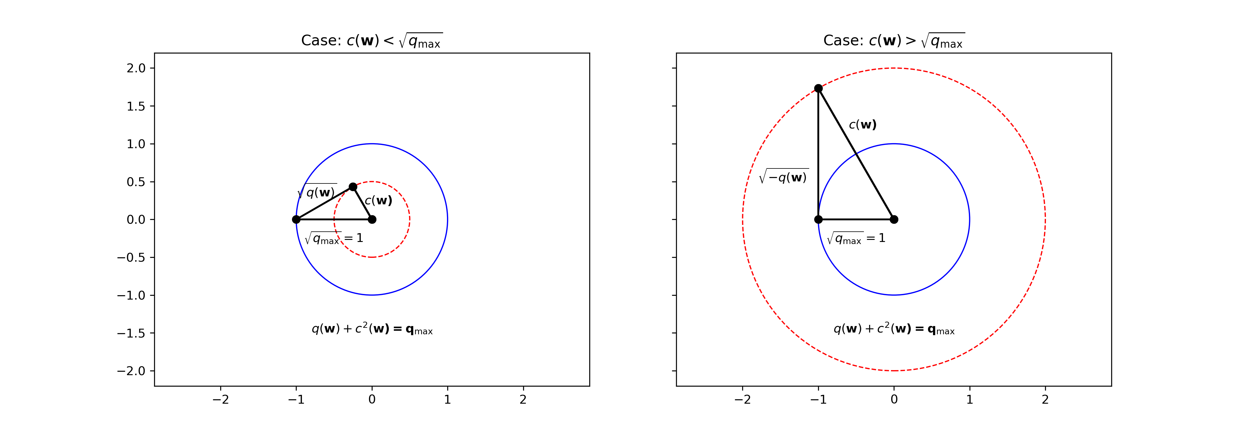
Figure 1: Pythagoras-style relationship between $c^{2}({\bf w})$ and $q({\bf w})$: the total sum is a constant. The blue circle represents embedding sphere of the MDRP and the origin is MDRP (see Thm. 3 for the detail). Its radius is $\sqrt{q_{\max}}$ and it is one in this illustration. The red circle represents those portfolios that have the same centrality $c({\bf w})$. When the red circle is inside the blue circle, the length of the hypotenuse is $\sqrt{q_{\max}}$. Otherwise, the length of the hypotenuse is $c({\bf w})$ in the right-angle triangle.

Moreover, the centrality is related to a weighted norm of ${\bf w}$. This link between the DR of a portfolio and its weighted norm brings out a new perspective of DR based portfolios. To put it another way, norm-weighted portfolios [8, 13] implicitly impose a condition on the diversification return. Hence, the much studied norm-regularized portfolios [8, 13] provide another strong motivation for a systematic study of optimal DR portfolio, echoing the empirical research on MDRP in [21].

The maximum diversification ratio portfolio (MDP) of Choueufaty and Coignard [6], which is behind several FSTE 100 products [3], is often confused with MDRP (their names are very similar). In fact, they are closely related. For the long-only case (portfolio weights are nonnegative), the gap between the objectives of the two portfolios can be quantitatively bounded and the gap can be small. This is well illustrated in the numerical part, where MDP is shown to be one of clustered portfolios.

The paper is organized as follows. The next section formally introduces the DR of a portfolio and provides the new characterization (1) relating the DR to the centrality of the portfolio, see Prop. 5. In Section 3, we study the most efficient DR portfolio under a given risk level and characterize the efficient DR curve as a strongly concave function, see Prop. 7. We further prove the separation theorem (Thm. 9) that states that any portfolio on the efficient DR curve can be represented by a simple mixture of MVP and MDRP. In Section 4, we study the DR representation of Markowitz efficient portfolios and characterize its relationship with the efficient DR curve. The relationship is graphically represented in Fig. 3, very similar to the classical graphical representation of the efficient frontier for the mean-variance model. We also extend this comparison study to the case of including a risk-free asset. We demonstrate the behaviour of the DR portfolios for DAX30 Index stocks in Section 5. The paper concludes in Section 6.

Notation: Through the paper, a boldfaced lower letter denotes a column vector. For example, ${\bf w}\in\Re^{n}$ is a column vector of dimension $n$. Its transpose ${\bf w}^{\top}$ is a row vector. Let $V$ denotes the covariance matrix of the returns of $n$ assets. Let $\eta$ denote its diagonal (column) vector of $V$, i.e., $\eta:=\mbox{diag}(V)$, where “$:=$” means “define”. From $V$, we define a new matrix:

$$D:=\frac{1}{2}\Big{(}\eta^{\top}{\bf 1}_{n}+{\bf 1}_{n}\eta^{\top}\Big{)}-V,$$

where ${\bf 1}_{n}$ is the column vector of all ones of dimension $n$. The $n\times n$ identity matrix is denoted by $I_{n}$. We will see in the next section that the properties of $D$ play an important role in our analysis. When $V$ is nonsingular, so is $D$ by [26, Lemma 2.3]. In this case, we let ${\bf w}_{\mbox{mvp}}$ denote the minimum variance portfolio

$${\bf w}_{\mbox{mvp}}:=\frac{V^{-1}{\bf 1}_{n}}{{\bf 1}_{n}^{\top}V^{-1}{\bf 1}_{n}}\quad\mbox{and}\quad\sigma^{2}_{\mbox{mvp}}=\frac{1}{{\bf 1}_{n}^{\top}V^{-1}{\bf 1}_{n}},$$

where $\sigma^{2}_{\mbox{mvp}}$ is the variance of MVP. Throughout, $\|\cdot\|$ denotes the Euclidean norm.

2 New Perspective of Diversification Return

Let us first recall the definition of DR of a portfolio.

Definition 1

[1] Suppose there are $n$ assets whose covariance matrix of their returns is denoted by $V$. The diversification return of a portfolio ${\bf w}$ satisfying the budget constraint ${\bf 1}_{n}^{\top}{\bf w}=1$ is defined by

$$q_{V}({\bf w}):=\frac{1}{2}\Big{(}\eta^{\top}{\bf w}-{\bf w}^{\top}V{\bf w}\Big{)}\qquad\mbox{with}\ \ \eta:=\mbox{diag}(V).$$

We often drop the dependence of $q$ on $V$ for simplicity.

In words, the diversification return is half of the difference between the weighted-average variance of the assets in the portfolio and the portfolio variance, see also [21, Eq. (9)]. We note that the factor $1/2$ in the definition of the diversification return is important. Mathematically, it results from the second-order Taylor expansion of the expected return of a portfolio, see [1].

In this part, we explain a peculiar phenomenon about DR. Different representation of a portfolio may have different DR depending how the portfolio is decomposed. We then derive an identity relating the centrality of a portfolio to its DR. This identity will explain why and how DR may be negative.

2.1 The matter of size

Let us use an example to demonstrate the fact that DR of a portfolio depends on how many assets are in it.

Example 2

Suppose we have two independent risky assets $S_{1}$ and $S_{2}$, whose covariance matrix is the identity matrix. Suppose there is also a riskfree asset $S_{0}$. We consider a portfolio ${\bf w}_{m}:=(1/2,1/4,1/4)^{\top}$ investing $50\%$ of the wealth to $S_{0}$ and $25\%$ each to the two risky assets. The covariance matrix of the three assets is

$$V=\left[\begin{array}[]{ccc}0&0&0\\ 0&1&0\\ 0&0&1\end{array}\right]\quad\mbox{with}\quad\eta=\left[\begin{array}[]{c}0\\ 1\\ 1\end{array}\right].$$

The DR of the portfolio is $q_{V}({\bf w}_{m})=\frac{1}{2}(1/2-1/8)=\frac{3}{16}$.

Now consider the equal-weight portfolio of the two risky asset ${\bf w}_{\mbox{ew}}=(1/2,1/2)^{\top}$. Its variance is $\sigma^{2}_{\mbox{ew}}=1/2$. Then the portfolio ${\bf w}_{m}$ can be regarded as investing $50\%$ to $S_{0}$ and $50\%$ to ${\bf w}_{\mbox{ew}}$. The new representation of ${\bf w}_{m}$ and its covariance matrix of the assets $S_{0}$ and ${\bf w}_{\mbox{ew}}$ are given below:

$${\bf w}_{m}=\left(\begin{array}[]{c}1/2\\ \frac{1}{2}{\bf w}_{\mbox{ew}}\end{array}\right),\qquad\widetilde{V}=\left[\begin{array}[]{cc}0&0\\ 0&1/2\end{array}\right]\quad\mbox{and}\quad\widetilde{\eta}=\left[\begin{array}[]{c}0\\ 1/2\end{array}\right].$$

Then the DR of ${\bf w}_{m}$ can also be calculated as $q_{\widetilde{V}}({\bf w}_{m})=\frac{1}{2}(1/4-1/8)=\frac{1}{16}$.

On the surface, it seems that two different DRs of the same portfolio ${\bf w}_{m}$ in Example 2 are due to the fact that two different covariance matrices are being used. On a deep level, it is because the DR of a portfolio measures the difference between the expected return of the portfolio and its second-order approximation through the expected returns of its constituents. Hence, the number of its constitutes is vital in computing DR. For $q_{V}({\bf w}_{m})$, there are three assets while $q_{\widetilde{V}}({\bf w}_{m})$ only used two (one is $S_{0}$ and the other is ${\bf w}_{\mbox{ew}}$). Therefore, it is only meaningful to discuss DR after the number of the assets involved has been decided.

2.2 Centrality of portfolio

This part introduces an important concept called the centrality of portfolio and study its relationship with the DR of the portfolio. For any portfolio ${\bf w}$ satisfying the budget constraint ${\bf 1}_{n}^{\top}{\bf w}=1$, its DR can be represented as follows:

$$q({\bf w})=\frac{1}{2}\eta^{\top}{\bf w}-\frac{1}{2}{\bf w}^{\top}V{\bf w}=\frac{1}{2}{\bf w}^{\top}\underbrace{\Big{(}(\eta{\bf 1}_{n}^{\top}+{\bf 1}_{n}\eta^{\top})/2-V\Big{)}}_{=\;D}{\bf w}$$

Recall that $\eta=\mbox{diag}(V)$. This implies that the diagonal of $D$ are zeros and all its elements $D_{ij}\geq 0$. In fact, $D$ is Euclidean Distance Matrix (EDM) [26, Lemma 2.2]. This means that there exist a set of points ${\bf x}_{i}$, $i=1,\ldots,n$ in the Euclidean space $\Re^{k}$ for some $k>0$ such that

$$\|{\bf x}_{i}-{\bf x}_{j}\|^{2}=D_{ij},\qquad i,j=1,\ldots,n.$$

Those points are called the embedding points of $D$ because their pairwise squared Euclidean distances recover the elements in $D$. This embedding result can be traced back to Schoenberg [29] and Young and Householder [34]. Obviously, there exist infinitely many such embedding points because shift and rotation transformations do not change pairwise distances. There is one special set of embedding points that are useful in characterizing the MDRP. We explain how we derive those points.

In [26, Thm. 3.1], it is showed that

$${\bf w}_{\mbox{mdrp}}=\frac{D^{-}{\bf 1}_{n}}{{\bf 1}_{n}^{\top}D^{-}{\bf 1}_{n}},$$

where $D^{-}$ can be chosen as any generalized inverse of $D$ satisfying $DD^{-}D=D$ and $D^{-}DD^{-}=D^{-}$. That is, ${\bf w}_{\mbox{mdrp}}$ does not depend on the choice of $D^{-}$. Let

$${\bf s}:={\bf w}_{\mbox{mdrp}},\quad J_{{\bf s}}:=I_{n}-{\bf s}{\bf 1}_{n}^{\top}\quad\mbox{and}\quad B:=-\frac{1}{2}J_{{\bf s}}^{\top}DJ_{{\bf s}}.$$ (2)

According to the theory of EDM [15], the matrix $B$ is positive semidefinite. Suppose it has the following spectral decomposition:

$$B=[{\bf p}_{1},\ldots,{\bf p}_{k}]\left[\begin{array}[]{ccc}\lambda_{1}&&\\ &\ddots&\\ &&\lambda_{k}\end{array}\right]\left[\begin{array}[]{c}{\bf p}_{1}^{\top}\\ \vdots\\ {\bf p}_{k}^{\top}\end{array}\right],$$ (3)

where $\lambda_{1}\geq\cdots\geq\lambda_{k}>0$ are the positive eigenvalues of $B$ and ${\bf p}_{i}\in\Re^{n}$ are the corresponding orthonormal eigenvectors. Let

$$X:=[{\bf x}_{1},\ldots,{\bf x}_{n}]=\left[\begin{array}[]{ccc}\sqrt{\lambda_{1}}&&\\ &\ddots&\\ &&\sqrt{\lambda_{k}}\end{array}\right]\left[\begin{array}[]{c}{\bf p}_{1}^{\top}\\ \vdots\\ {\bf p}_{k}^{\top}\end{array}\right].$$ (4)

Then $B=X^{\top}X$ and ${\bf x}_{i}$, $i=1,\ldots,n$ are one set of embedding points of $D$. Moreover, the following are proved in [26].

Theorem 3

[26, Thm. 3.1] Let $q_{\max}:=q({\bf w}_{mdrp})$ be the maximum diversification return of MDRP. Let the embedding points ${\bf x}_{i}$, $i=1,\ldots,n$ be obtained by (4). Then $q_{\max}=\frac{1}{2{\bf 1}_{n}^{\top}D^{-}{\bf 1}_{n}}>0$ and those embedding points sit on the sphere of centered at the origin with the radius $\sqrt{q_{\max}}$, i.e.,

$$\|{\bf x}_{i}\|=\sqrt{\frac{1}{2{\bf 1}_{n}^{\top}D^{-}{\bf 1}_{n}}}=\sqrt{q_{\max}},\qquad i=1,\ldots,n.$$

Furthermore, the origin is the ${\bf s}$-weighted center of the embedding points:

$$0=s_{1}{\bf x}_{1}+s_{2}{\bf x}_{2}+\cdots+s_{n}{\bf x}_{n}\quad\mbox{or equivalently}\quad X{\bf s}=0.$$

Geometrically, Thm. 3 means that the origin represents MDRP. For any other portfolio ${\bf w}$, the ${\bf w}$-weighted centre of the embedding points is away from the origin. Its distance from the origin measures how far it is from MDRP. We call the distance portfolio centrality.

Definition 4

(Portfolio centrality) Let the matrix $B$ be defined by (2). For a given portfolio ${\bf w}$, its centrality is defined by

$$c({\bf w}):=\sqrt{{\bf w}^{\top}B{\bf w}}.$$

Remark 1

(Interpretation of centrality) Let us explain why $c({\bf w})$ measures the centrality of portfolio ${\bf w}$ with respect to MDRP. Using (4), we have

$$c^{2}({\bf w})={\bf w}^{\top}B{\bf w}={\bf w}^{\top}X^{\top}X{\bf w}=\|X{\bf w}\|^{2}.$$

Therefore, $c({\bf w})=\|X{\bf w}\|$. From Thm. 3, we have $X{\bf s}=0$, which is the centre of the embedding sphere. On the other hand, $X{\bf w}$ represents the embedding point of portfolio ${\bf w}$ in the embedding space spanned by $\{{\bf x}_{i}\}$. The quantity $\|X{\bf w}\|$ measures how far it is from the origin.

Another interesting interpretation is as follows. The decomposition (3) gives rise to $k$ principle dimensions ${\bf p}_{i}$, $i=1,\ldots,k$. For a given portfolio ${\bf w}$, we may compute its principle coordinates

$$\widetilde{w}_{i}:={\bf p}_{i}^{\top}{\bf w},\quad i=1,\ldots,n.$$

Denote this new point by $\widetilde{{\bf w}}$. Obviously, the length remains the same: $\|\widetilde{{\bf w}}\|=\|{\bf w}\|$. The centrality considers the weighted length by the eigenvalues:

$$c({\bf w})=\sqrt{\lambda_{1}\widetilde{w}_{1}^{2}+\cdots+\lambda_{k}\widetilde{w}_{k}^{2}}.$$

This interpretation is closely related to the principle coordinate analysis, initially studied by Gower [14].

Since the centrality measures how far a portfolio is from the origin and the origin represents the maximum diversification return, we like to know if the higher centrality means lower diversification return. The following result proves it is the case.

Proposition 5

For any portfolio ${\bf w}$ satisfying ${\bf 1}_{n}^{\top}{\bf w}=1$, it holds

$$c^{2}({\bf w})+q({\bf w})=q_{\max}.$$ (5)

Proof. We first note from Thm. 3 that

$$q_{\max}=q({\bf s})=\frac{1}{2}\frac{1}{{\bf 1}^{n}D^{-}{\bf 1}_{n}}.$$

For any portfolio ${\bf w}$, it is easy to see

$$J_{{\bf s}}{\bf w}=\Big{(}I_{n}-{\bf s}{\bf 1}_{n}^{\top}\Big{)}{\bf w}={\bf w}-{\bf s}\qquad(\mbox{using }{\bf 1}_{n}^{\top}{\bf w}=1)$$

and

$${\bf w}^{\top}D{\bf s}=\frac{{\bf w}^{\top}DD^{-}{\bf 1}_{n}}{{\bf 1}_{n}^{\top}D^{-}{\bf 1}}=\frac{{\bf w}^{\top}{\bf 1}_{n}}{{\bf 1}_{n}^{\top}D^{-}{\bf 1}}=\frac{1}{{\bf 1}_{n}^{\top}D^{-}{\bf 1}}=2q({\bf s}),$$

where the second equation used the fact $DD^{-}{\bf 1}_{n}={\bf 1}_{n}$, which was established in [16, Thm. 2] for any Euclidean distance matrix. Using those facts, we compute $c^{2}({\bf w})$ as follows:

$$c^{2}({\bf w}) = {\bf w}^{\top}B{\bf w}=-\frac{1}{2}{\bf w}^{\top}J_{{\bf s}}^{\top}DJ_{{\bf s}}{\bf w}$$

$$= -\frac{1}{2}({\bf w}-{\bf s})^{\top}D({\bf w}-{\bf s})=-\frac{1}{2}{\bf w}^{\top}D{\bf w}+{\bf w}^{\top}D{\bf s}-\frac{1}{2}{\bf s}^{\top}D{\bf s}$$

$$= -q({\bf w})+2q({\bf s})-q({\bf s})=-q({\bf w})+q({\bf s}).$$

Noticing $q({\bf s})=q_{\max}$, we derived the claimed identity. $\Box$

The identity (5) has a significant implication: for a portfolio, if its weighted center is further away from the origin, then its centrality increases and consequently its diversification return decrease. The sum of the diversification return of a portfolio and its squared centrality is a constant, which is the maximum diversification return $q_{\max}$. We recall that the diversification return can be cast as Rao’s quadratic entropy [28, 26], and entropy is generally one kind of energy. In this sense, the considered $n$ risky assets have a constant energy and the energy decomposes into two parts for any portfolio. One part is allocated to the diversification return of the portfolio and the other part is for its centrality (distance from the location of total energy). At any point of state, the two types of energy can transfer to each other. But their total sum remains constant. It becomes an art of portfolio construction to decide which state an investor would like to stay and invest.

2.3 Norm-regularized portfolios are diversified

Since the seminar work of Jaganathan and Ma [19], norm constrained portfolio construction has gained significant attention, see, e.g., [8, 13]. Our key message below is that norm constraints implicitly require the diversification return to be above a certain level. Let us use the global minimum variance portfolio (GMVP) under a general norm constraint studied in [8] to demonstrate this implication.

$$\min\frac{1}{2}{\bf w}^{\top}V{\bf w},\quad\mbox{s.t.}\quad{\bf 1}_{n}^{\top}{\bf w}=1,\ \ \|{\bf w}\|_{A}\leq\tau,$$ (6)

for some $\tau>0$, where $\|{\bf w}\|_{A}$ is the A-norm of ${\bf w}$ defined by $\|{\bf w}\|_{A}:=\sqrt{{\bf w}^{\top}A{\bf w}}$ with $A$ being symmetric and positive definite. In particular, when $A=I_{n}$ (the identity matrix), $\|{\bf w}\|_{A}=\|{\bf w}\|$ becomes the Euclidean norm (also known as the $\ell_{2}$-norm in [33, 35]).

Recall the matrix $B$ is defined by (2). Let $\beta^{2}:=\lambda_{\min}(A)/\lambda_{\max}(B)>0,$ where $\lambda_{\max}(B)$ is the largest eigenvalue of $B$ and $\lambda_{\min}(A)$ is the smallest eigenvalue of $A$. Then the matrix $(A-\beta^{2}B)$ is positive semidefinite. Consequently, we have

$$\|{\bf w}\|_{A}\geq\beta\|{\bf w}\|_{B}=\beta c({\bf w}).$$

Therefore, the norm constraint in (6) implies

$$c({\bf w})\leq\tau/\beta,$$

or equivalently by using the identity (5)

$$q({\bf w})\geq q_{\max}-(\tau/\beta)^{2}.$$

This means that any $A$-norm constraint in (6) actually requires the diversification return of the portfolio be above a threshold. Interestingly, Carmichael et. al. [3] imposed a diversification return constraint of the type $q({\bf w})\geq\tau$ in their portfolio construction and observed strong out-of-sample performance, similar to what has been observed in [8]. The connection between the norm constraint and the diversification return constraint explains why both can lead to similar out-of-sample performance.

We now borrow an example from [26] to illustrate the main results in this section.

Example 6

[26, Example 3.1] Suppose there are three risky assets $S_{i}$, $i=1,2,3$, whose covariance matrix $V$, the corresponding distance matrix $D$ and its inverse $D^{-1}$ are respectively given by

$$V=\frac{1}{9}\left[\begin{array}[]{ccc}11&8&8\\ 8&23&-4\\ 8&-4&23\end{array}\right],\qquad D=\left[\begin{array}[]{ccc}0&1&1\\ 1&0&3\\ 1&3&0\end{array}\right],\qquad D^{-1}=\frac{1}{6}\left[\begin{array}[]{ccc}-9&3&3\\ 3&-1&1\\ 3&1&-1\end{array}\right].$$

We note that $V$ is also nonsingular. It follows from Thm. 3 that the MDRP is ${\bf w}_{\mbox{mdrp}}=(-1,1,1)^{\top}.$ The corresponding embedding points are ${\bf x}_{1}=(1,0)^{\top},$ ${\bf x}_{2}=(1/2,\sqrt{3}/2)^{\top},$ and ${\bf x}_{3}=(1/2,-\sqrt{3}/2)^{\top}.$ They lie on the sphere of radius $R=1$ centred at the origin, see Fig. 2, where we also indicated the minimum variance portfolio ${\bf w}_{\mbox{mvp}}=(1/3,1/3,1/3)^{\top}$ with $c_{\mbox{mvp}}=2/3$ or equivalently $q_{\mbox{mvp}}=1-(2/3)^{2}=5/9$. Outside the unit circle, it holds $c({\bf w})>1$, which implies negative diversification returns for those portfolios. The triangle formed by ${\bf x}_{1}$, ${\bf x}_{2}$ and ${\bf x}_{3}$ is the region of portfolios with nonnegative weights because the region is the convex hull of the three points. Outside of the triangle, there must be at least one negative weight. For example, MDRP is outside the triangle and its first weight is ($-1$). It is also straightforward to impose constraints on the diversification return $q({\bf w})$. For example, if we require the DR to be nonnegative, then we have

$$q({\bf w})\geq 0\quad\Longleftrightarrow\quad c^{2}({\bf w})\leq 1\quad\Longleftrightarrow\quad\|{\bf w}\|_{B}\leq 1\quad\Longleftrightarrow\quad\frac{1}{4}(1+w_{1})^{2}+\frac{3}{4}(w_{2}-w_{3})^{2}\leq 1.$$

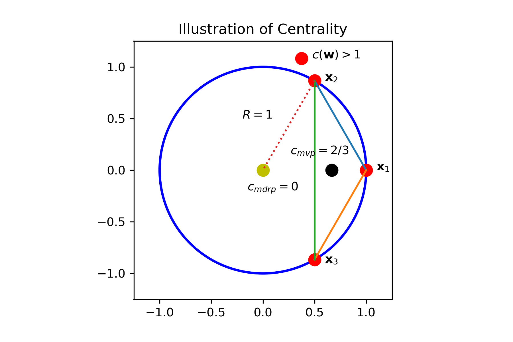
Figure 2: Asset and portfolio representation in the embedding space for the data in Example 6: the sphere is centred at the origin with $R=1$ and the three embedding points on the sphere of the assets are ${\bf x}_{1}$, ${\bf x}_{2}$ and ${\bf x}_{3}$. Three portfolios are: MDRP (the origin), MVP (dot in black with its centrality being $2/3$), a portfolio outside of the sphere ($c({\bf w})>1$).

We will see the identity (5) greatly facilitate our derivation of the separation theorem below.

3 Efficient Frontier of DRP

In the proceeding section, we established the identity (5), which means that maximizing the diversification return is equivalent to minimizing the centrality, which in turn is closely related to norm-regularization of the portfolio weight. In this part, we study the maximum DR portfolio under a given risk level $\sigma^{2}$ and then establish a separation theorem. From now on, we assume that $V$ is nonsingular. Consequently, the Euclidean distance matrix $D$ is also nonsingular. Moreover, the maximum diversification return portfolio has the following closed-form solution:

$${\bf w}_{\mbox{mdrp}}=\frac{D^{-1}{\bf 1}_{n}}{{\bf 1}_{n}^{\top}D^{-1}{\bf 1}_{n}}=\left(1-\frac{{\bf 1}_{n}^{\top}V^{-1}\eta}{2}\right)\frac{V^{-1}{\bf 1}_{n}}{{\bf 1}_{n}^{\top}V^{-1}{\bf 1}_{n}}+\frac{1}{2}V^{-1}\eta.$$ (7)

The first representation above is in terms of $D^{-1}$, and the second is in terms of $V^{-1}$ and is also obtained in [21, Eq (18)].

3.1 The efficient DR curve

The optimization problem we study is defined as follows:

$${\bf w}(\sigma):=\arg\max q({\bf w}),\quad\mbox{s.t.}\quad{\bf 1}_{n}^{\top}{\bf w}=1,\ \ {\bf w}^{\top}V{\bf w}=\sigma^{2}.$$ (8)

In particular, we study the relationship between $q({\bf w}(\sigma))$ and $\sigma$ so that the optimal portfolios ${\bf w}(\sigma)$ form a dominating smooth and concave curve in the $(\sigma,q)$ diagram. This development is much in the spirit of Merton’s classical contribution [22] to the mean-variance model.

Under the condition ${\bf 1}_{n}^{\top}{\bf w}=1$, the objective $q({\bf w})$ becomes

$$q({\bf w})=\frac{1}{2}{\bf w}^{\top}D{\bf w}=\frac{1}{2}\eta^{\top}{\bf w}-\frac{1}{2}{\bf w}^{\top}V{\bf w}=\frac{1}{2}\eta^{\top}{\bf w}-\frac{1}{2}\sigma^{2}.$$ (9)

Problem (8) reduces to

$${\bf w}(\sigma):=\arg\max\frac{1}{2}\eta^{\top}{\bf w},\quad\mbox{s.t.}\quad{\bf 1}_{n}^{\top}{\bf w}=1,\ \ {\bf w}^{\top}V{\bf w}=\sigma^{2}.$$ (10)

This is to maximize a linear function over the surface of an ellipsoid. Therefore, the optimization can be done over the ellipsoid, leading to the following convex optimization problem:

$${\bf w}(\sigma):=\arg\max 2\eta^{\top}{\bf w},\quad\mbox{s.t.}\quad{\bf 1}_{n}^{\top}{\bf w}=1,\ \ {\bf w}^{\top}V{\bf w}\leq\sigma^{2}.$$ (11)

We note the small change in the objective: we used $2\eta^{\top}{\bf w}$ instead of $(\eta^{\top}{\bf w})/2$. This change is a positive scaling of the objective function and hence it won’t change the optimal solution ${\bf w}(\sigma)$. The benefit of this change will become clear when we study the KKT condition of (11). We also note that it is necessary to require $\sigma^{2}\geq\sigma_{\mbox{mvp}}^{2}$ (the variance of the minimum variance portfolio (MVP)) for ${\bf w}(\sigma)$ to be well defined. We have the following result.

Proposition 7

For $\sigma^{2}\geq\sigma_{\mbox{mvp}}^{2}$, we have

$$\eta^{\top}{\bf w}(\sigma)=\rho\sqrt{\sigma^{2}-\sigma_{\mbox{mvp}}^{2}}+\frac{{\bf 1}_{n}^{\top}V^{-1}\eta}{{\bf 1}_{n}^{\top}V^{-1}{\bf 1}_{n}},\ \ \mbox{with}\ \ \rho:=\sqrt{\eta^{\top}V^{-1}\eta-({\bf 1}_{n}^{\top}V^{-1}\eta)^{2}/{\bf 1}_{n}^{\top}V^{-1}{\bf 1}_{n}}.$$ (12)

Moreover, the diversification return of ${\bf w}(\sigma)$, denoted by $q_{\mbox{dr}}(\sigma):=q({\bf w}(\sigma))$ is given by

$$q_{\mbox{dr}}(\sigma)=-\frac{1}{2}\Big{(}\sqrt{\sigma^{2}-\sigma_{\mbox{mvp}}^{2}}-\rho/2\Big{)}^{2}+\frac{1}{8}\rho^{2}+q_{\mbox{mvp}}.$$ (13)

In particular, when $\sigma=\sigma_{\mbox{mvp}}$, the DR of the minimum variance portfolio, denoted by $q_{\mbox{mvp}}$ is given by

$$q_{\mbox{mvp}}=\frac{1}{2}\Big{(}{\bf 1}_{n}^{\top}V^{-1}\eta-1\Big{)}\sigma_{\mbox{mvp}}^{2}.$$ (14)

Proof. For the case $\sigma^{2}=\sigma_{\mbox{mvp}}^{2}$, the feasible region of (11) has only one point, which is ${\bf w}_{\mbox{mvp}}$. The formula (12) is easily versified because ${\bf w}(\sigma)={\bf w}_{\mbox{mvp}}$.

We now consider the case $\sigma^{2}>\sigma_{\mbox{mvp}}^{2}$. For this case, we note that the Slater condition is satisfied. One can verify that ${\bf w}_{\mbox{mvp}}$ is in the relative interior of the feasible region of (11). Therefore, the KKT condition holds at ${\bf w}={\bf w}(\sigma)$:

$$-2\eta-2\lambda{\bf 1}_{n}+2\beta V{\bf w}=0,\quad{\bf 1}_{n}^{\top}{\bf w}=1,\quad\beta\geq 0,\ \ {\bf w}^{\top}V{\bf w}\leq\sigma^{2}\ \ \mbox{and}\ \ \beta({\bf w}^{\top}V{\bf w}-\sigma^{2})=0.$$ (15)

where $(2\lambda)$ is the Lagrange multiplier corresponding to ${\bf 1}_{n}^{\top}{\bf w}=1$ and $\beta\geq 0$ is the Lagrange multiplier for the ellipsoid constraint. We solve the KKT condition (15) below.

We first remove the trivial case that $\eta$ is proportional to ${\bf 1}_{n}$, i.e., $\eta=\gamma{\bf 1}_{n}$ for some $\gamma>0$. In this case, the objective function is constant $2\gamma$ and hence any point in the feasible region of (11) is optimal. It is easy to verify that the formula in (12) gives the correct value for $\eta^{\top}{\bf w}(\sigma)$. Therefore, we assume $\eta\not=\gamma{\bf 1}_{n}$ for any $\gamma>0$. It follows from the first equation in (15) that

$$\beta{\bf w}=V^{-1}(\eta+\lambda{\bf 1}_{n})\not=0\qquad(\mbox{because}\ \eta+\lambda{\bf 1}_{n}\not=0,\ \forall\ \lambda\in\Re).$$

Hence $\beta\not=0$. By using the second equation in (15), we get

$${\bf w}=\frac{1}{\beta}\Big{(}V^{-1}\eta+\lambda V^{-1}{\bf 1}_{n}\Big{)}\quad\mbox{and}\quad\lambda=\frac{1}{{\bf 1}_{n}^{\top}V^{-1}{\bf 1}_{n}}\beta-\frac{{\bf 1}_{n}^{\top}V^{-1}\eta}{{\bf 1}_{n}^{\top}V^{-1}{\bf 1}_{n}}.$$

Since ${\bf w}(\sigma)$ must be on the boundary of the ellipsoid, we substitute ${\bf w}$ into the equation ${\bf w}^{\top}V{\bf w}=\sigma^{2}$ to get after simplification:

$$\left(\sigma^{2}-\sigma_{\mbox{mvp}}^{2}\right)\beta^{2}=\eta^{\top}V^{-1}\eta-\frac{({\bf 1}_{n}^{\top}V^{-1}\eta)^{2}}{{\bf 1}_{n}^{\top}V^{-1}{\bf 1}_{n}}$$

By Cauchy-Schwartz inequality, we have $({\bf 1}_{n}^{\top}V^{-1}\eta)^{2}\leq(\eta^{\top}V^{-1}\eta)({\bf 1}_{n}^{\top}V^{-1}{\bf 1}_{n})$. Therefore, the right-hand side of the above equation is nonnegative. Given $\beta>0$, we have

$$\beta=\sqrt{\frac{\eta^{\top}V^{-1}\eta-({\bf 1}_{n}^{\top}V^{-1}\eta)^{2}/{\bf 1}_{n}^{\top}V^{-1}{\bf 1}_{n}}{\sigma^{2}-\sigma_{\mbox{mvp}}^{2}}}.$$

We then can compute $\lambda$ in terms of $\beta$ and subsequently we get

$$\eta^{\top}{\bf w}(\sigma) = \frac{1}{\beta}\Big{(}\eta^{\top}V^{-1}\eta+\lambda\eta^{\top}V^{-1}{\bf 1}_{n}\Big{)}$$

$$= \frac{1}{\beta}\left(\eta^{\top}V^{-1}\eta+\frac{{\bf 1}_{n}^{\top}V^{-1}\eta}{{\bf 1}_{n}^{\top}V^{-1}{\bf 1}_{n}}\beta-\frac{({\bf 1}_{n}^{\top}V^{-1}\eta)^{2}}{{\bf 1}_{n}^{\top}V^{-1}{\bf 1}_{n}}\right)$$

$$= \frac{1}{\beta}\left(\eta^{\top}V^{-1}\eta-\frac{({\bf 1}_{n}^{\top}V^{-1}\eta)^{2}}{{\bf 1}_{n}^{\top}V^{-1}{\bf 1}_{n}}\right)+\frac{{\bf 1}_{n}^{\top}V^{-1}\eta}{{\bf 1}_{n}^{\top}V^{-1}{\bf 1}_{n}}.$$

Substituting $\beta$ into the last equation above yields the formula (12). We proved it for all cases.

It follows from (12) that

$$\eta^{\top}{\bf w}_{\mbox{mvp}}=\frac{{\bf 1}_{n}^{\top}V^{-1}\eta}{{\bf 1}_{n}^{\top}V^{-1}{\bf 1}_{n}}=({\bf 1}_{n}^{\top}V^{-1}\eta)\sigma^{2}_{\mbox{mvp}}\quad(\mbox{using the fact}\ \sigma^{2}_{\mbox{mvp}}=\frac{1}{{\bf 1}_{n}^{\top}V^{-1}{\bf 1}_{n}}),$$

which, together with (9) yields

$$q_{\mbox{mvp}}=-\frac{1}{2}\sigma^{2}_{\mbox{mvp}}+\frac{1}{2}\eta^{\top}{\bf w}_{\mbox{mvp}}=\frac{1}{2}({\bf 1}_{n}^{\top}V^{-1}\eta-1)\sigma^{2}_{\mbox{mvp}}.$$

This proves (14)). Equation (13) is simple application of (12) by noticing

$$q_{\mbox{dr}}(\sigma) = q({\bf w}(\sigma))=-\frac{1}{2}\sigma^{2}+\frac{1}{2}\eta^{\top}{\bf w}(\sigma)$$

$$= -\frac{1}{2}\sigma^{2}+\frac{1}{2}\rho\sqrt{\sigma^{2}-\sigma_{\mbox{mvp}}^{2}}+\frac{1}{2}\frac{{\bf 1}_{n}^{\top}V^{-1}\eta}{{\bf 1}_{n}^{\top}V^{-1}{\bf 1}_{n}}$$

$$= -\frac{1}{2}\Big{(}\sqrt{\sigma^{2}-\sigma_{\mbox{mvp}}^{2}}-\rho/2\Big{)}^{2}+\frac{1}{8}\rho^{2}+\underbrace{\frac{1}{2}({\bf 1}_{n}^{\top}V^{-1}\eta)\sigma^{2}_{\mbox{mvp}}-\frac{1}{2}\sigma^{2}_{\mbox{mvp}}}_{=\;q_{\mbox{mvp}}\ \mbox{by}\ \eqref{q_mvp}}.$$

$\Box$

We make the following remark, which includes some useful identities.

Remark 2

It is easy to verify that the function

$$f(x):=\left(\sqrt{x^{2}-x_{0}^{2}}-c\right)^{2}$$

is strongly convex for $x\geq x_{0}$ when $x_{0}>0$ and $c\geq 0$. Consequently, the function $q_{\mbox{dr}}(\sigma)$ is strongly concave in $\sigma$ for $\sigma\geq\sigma_{\mbox{mvp}}$. Solving the equation

$$0=q^{\prime}_{\mbox{dr}}(\sigma)=\frac{\rho}{2}\frac{\sigma}{\sqrt{\sigma^{2}-\sigma_{\mbox{mvp}}^{2}}}-\sigma$$ (16)

yields the maximum DR. The corresponding portfolio is ${\bf w}_{\mbox{mdrp}}$. The solution of (16) and the corresponding DR are given by

$$\sigma_{\mbox{mdrp}}^{2}=\sigma_{\mbox{mvp}}^{2}+\frac{\rho^{2}}{4}\quad\mbox{and}\quad q_{\mbox{mdrp}}=\frac{1}{8}\rho^{2}+q_{\mbox{mvp}}.$$ (17)

The concavity of $q_{\mbox{dr}}(\sigma)$ makes the efficient DR portfolios sit on the frontier of the $(\sigma,q)$ diagram, much like the classical efficient frontier of Markowitz Mean-Variance portfolios. Next, we are going to prove that the frontier can be obtained by combining the two portfolios: MVP and MDRP.

3.2 Separation Theorem

The main purpose of this part is to prove that in order to invest on the efficient frontier of DR, one only needs to invest in two portfolios: Minimum Variance Portfolio and Maximum Diversification Return Portfolio via their simple combination by specifying the level $\alpha$,

$${\bf w}_{\alpha}=\alpha{\bf w}_{\mbox{mdrp}}+(1-\alpha){\bf w}_{\mbox{mvp}}={\bf w}_{\mbox{mvp}}+\alpha({\bf w}_{\mbox{mdrp}}-{\bf w}_{\mbox{mvp}}),\quad\alpha\geq 0.$$ (18)

In the classical theory of Markowitz efficient frontier, this is known as the separation theorem [31] and [2, Thm. 5.2.1]. We establish the result by proving that the standard deviation ($\sigma$) and the diversification return ($q$) curve formed by the combined portfolio ${\bf w}(\alpha)$ is the same as $q_{\mbox{dr}}$.

Theorem 8

Let the constant $\rho$ be defined in (12). The optimal diversification return portfolio ${\bf w}(\sigma)$ of Problem (8) is given by

$${\bf w}(\sigma)=\alpha{\bf w}_{\mbox{mdrp}}+(1-\alpha){\bf w}_{\mbox{mvp}},\qquad\mbox{with}\quad\alpha:=\frac{2}{\rho}\sqrt{\sigma^{2}-\sigma^{2}_{\mbox{mvp}}}.$$

Proof. Let us consider the affine combination ${\bf w}_{\alpha}$ of the portfolios ${\bf w}_{\mbox{mdrp}}$ and ${\bf w}_{\mbox{mvp}}$ in (18). We will show once the variance level of ${\bf w}_{\alpha}$ is specified as $\sigma^{2}$, then $\alpha$ is uniquely decided and equals $(2/\rho)\sqrt{\sigma^{2}-\sigma^{2}_{\mbox{mvp}}}$ as stated in the result.

Let

$${\bf d}:={\bf w}_{\mbox{mdrp}}-{\bf w}_{\mbox{mvp}}=\frac{1}{2}V^{-1}\eta-\frac{{\bf 1}_{n}^{\top}V^{-1}\eta}{2}\times\frac{V^{-1}{\bf 1}_{n}}{{\bf 1}_{n}^{\top}V^{-1}{\bf 1}_{n}}$$ (19)

and $\sigma^{2}_{{\bf d}}$ be the variance of ${\bf d}$. It is easy to verify that

$$\sigma^{2}_{{\bf d}}={\bf d}^{\top}V{\bf d} = \left(\frac{1}{2}V^{-1}\eta-\frac{{\bf 1}_{n}^{\top}V^{-1}\eta}{2}\times\frac{V^{-1}{\bf 1}_{n}}{{\bf 1}_{n}^{\top}V^{-1}{\bf 1}_{n}}\right)^{\top}\left(\frac{1}{2}\eta-\frac{{\bf 1}_{n}^{\top}V^{-1}\eta}{2}\times\frac{{\bf 1}_{n}}{{\bf 1}_{n}^{\top}V^{-1}{\bf 1}_{n}}\right)$$ (20)

$$= \frac{1}{4}\rho^{2}$$

and

$${\bf d}^{\top}V{\bf w}_{\mbox{mvp}}=\left(\frac{1}{2}V^{-1}\eta-\frac{{\bf 1}_{n}^{\top}V^{-1}\eta}{2}\times\frac{V^{-1}{\bf 1}_{n}}{{\bf 1}_{n}^{\top}V^{-1}{\bf 1}_{n}}\right)^{\top}\frac{{\bf 1}_{n}}{{\bf 1}_{n}^{\top}V^{-1}{\bf 1}_{n}}=0.$$

Consequently, we have

$$\sigma^{2}={\bf w}_{\alpha}^{\top}V{\bf w}_{\alpha}=\sigma_{\mbox{mvp}}^{2}+\alpha^{2}\sigma^{2}_{{\bf d}}=\sigma_{\mbox{mvp}}^{2}+\frac{1}{4}\rho^{2}\alpha^{2}.$$

Given $\alpha\geq 0$, we have

$$\alpha=\frac{2}{\rho}\sqrt{\sigma^{2}-\sigma^{2}_{\mbox{mvp}}}.$$ (21)

Having established (21), we now compute the DR of ${\bf w}_{\alpha}$ and its centrality. For simplicity, let $q_{\alpha}:=q({\bf w}_{\alpha})$ and $c_{\alpha}:=c({\bf w}_{\alpha})$. We compute $q_{\alpha}$ through $c_{\alpha}$. It is important to note that the matrix $J_{{\bf s}}$ defined in (2) has the following property

$$J_{{\bf s}}{\bf w}_{\mbox{mdrp}}=J_{{\bf s}}{\bf s}=0.$$

This implies $B{\bf w}_{\mbox{mdrp}}=0$. We then have

$$c^{2}_{\alpha} = {\bf w}_{\alpha}^{\top}B{\bf w}_{\alpha}$$ (22)

$$= \alpha^{2}{\bf w}_{\mbox{mdrp}}^{\top}B{\bf w}_{\mbox{mdrp}}+2\alpha(1-\alpha){\bf w}_{\mbox{mvp}}^{\top}B{\bf w}_{\mbox{mdrp}}+(1-\alpha)^{2}{\bf w}_{\mbox{mvp}}^{\top}B{\bf w}_{\mbox{mvp}}$$

$$= (1-\alpha)^{2}{\bf w}_{\mbox{mvp}}^{\top}B{\bf w}_{\mbox{mvp}}=(1-\alpha)^{2}c^{2}_{\mbox{mvp}}$$

We now make use of the identity (5) twice. The first time is on $c_{\mbox{mvp}}$: the identity implies

$$c^{2}_{\mbox{mvp}}+q_{\mbox{mvp}}=q_{\mbox{mdrp}}\qquad\mbox{(note $q_{\mbox{mdrp}}$ is $q_{\max}$)}.$$

It follows from (17) that

$$c^{2}_{\mbox{mvp}}=\frac{1}{8}\rho^{2}.$$ (23)

The second time to use the identity (5) is on $c_{\alpha}$ to get

$$q_{\alpha}=q_{\mbox{mdrp}}-c^{2}_{\alpha}\stackrel{{\scriptstyle(\ref{cw2})}}{{=}}q_{\mbox{mdrp}}-(1-\alpha)^{2}c^{2}_{\mbox{mvp}}\stackrel{{\scriptstyle(\ref{cmvp2})}}{{=}}q_{\mbox{mdrp}}-\frac{\rho^{2}}{8}(1-\alpha)^{2}.$$

Substituting $\alpha$ in (21) and $q_{\mbox{mdrp}}$ in (17) into above equation yields (after some simplification)

$$q_{\alpha}=-\frac{1}{2}\left(\sqrt{\sigma^{2}-\sigma^{2}_{\mbox{mvp}}}-\frac{\rho}{2}\right)^{2}+\frac{1}{8}\rho^{2}+q_{\mbox{mvp}}$$

Using formula (14) for $q_{\mbox{mvp}}$, $q_{\alpha}$ is just $q_{\mbox{dr}}$ in (13). This is to say that the $(\sigma,q)$ curve formed by the portfolio ${\bf w}_{\alpha}$ is same as that of the optimal portfolio ${\bf w}(\sigma)$. The correspondences between $\alpha$ and $\sigma$ is given by (21). This proves the theorem. $\Box$

It is worth noting that the meaningful range for $\alpha$ is $0\leq\alpha\leq 1$. This is because when $\alpha>1$, the corresponding portfolio has larger standard deviation due to (21) than MDRP (i.e., $\sigma>\sigma_{\mbox{mdrp}})$, but with less DR.

4 Relationship of Two Efficient Frontiers

In this part, we answer the interesting question where the classical efficient frontier would fit in the $(\sigma,q)$ diagram and how far it would be from the DR frontier just studied. We also investigate the portfolio that has the highest diversification return on the efficient frontier.

4.1 The $(\sigma,q)$ curve of MV efficient portfolios

Let us briefly review some key facts about the efficient portfolios in Markowitz’s Mean-Variance model. We denote the expected return vector of the $n$ risky assets by $\overline{{\bf r}}$. For a given level of risk $\sigma^{2}$, the MV model seeks the optimal portfolio by solving the following problem:

$${\bf w}_{\mbox{mv}}(\sigma):=\arg\max\;\overline{{\bf r}}^{\top}{\bf w},\qquad\mbox{s.t.}\quad{\bf 1}_{n}^{\top}{\bf w}=1,\quad{\bf w}^{\top}V{\bf w}\leq\sigma^{2}.$$ (24)

To remove the trivial case, we assume that $\overline{{\bf r}}$ is not proportional to ${\bf 1}_{n}$. Otherwise, all risky assets have the same expected returns and as a consequence that all portfolios have the same return. The classical portfolio theory says that all the optimal portfolios ${\bf w}_{\mbox{mv}}$ as $\sigma$ varies form a efficient frontier in the standard deviation and return diagram. Moreover, those portfolios have the following representation [2, Corollary. 4.2.1]:

$${\bf w}_{\mbox{mv}}(\sigma)={\bf w}_{\mbox{mvp}}+\alpha{\bf w}_{o},\quad\mbox{with}\ \ \alpha=\sqrt{\sigma^{2}-\sigma_{mvp}^{2}},$$

where

$${\bf w}_{o}:=\frac{V^{-1}\Big{(}\overline{{\bf r}}-\frac{b}{a}{\bf 1}_{n}\Big{)}}{\sqrt{\Big{(}\overline{{\bf r}}-\frac{b}{a}{\bf 1}_{n}\Big{)}^{\top}V^{-1}\Big{(}\overline{{\bf r}}-\frac{b}{a}{\bf 1}_{n}\Big{)}}},\quad a:={\bf 1}_{n}^{\top}V^{-1}{\bf 1}_{n},\quad b:={\bf 1}_{n}^{\top}V^{-1}\overline{{\bf r}}.$$ (25)

In [2], ${\bf w}_{o}$ is called a self-financing portfolio and is normalized because of the following facts:

$${\bf 1}_{n}^{\top}{\bf w}_{o}=0\qquad\mbox{and}\qquad{\bf w}_{o}^{\top}V{\bf w}_{o}=1.$$ (26)

We denote the diversification return of ${\bf w}_{\mbox{mv}}(\sigma)$ by $q_{\mbox{ef}}(\sigma)$ (here $q_{\mbox{ef}}$ means it is the diversification return on the efficient frontier of the mean-variance model).

We now calculate $q_{\mbox{ef}}$ by using the above facts and the formula (9):

$$q_{\mbox{ef}}(\sigma) = -\frac{1}{2}\sigma^{2}+\frac{1}{2}\eta^{\top}{\bf w}_{\mbox{mv}}(\sigma)$$ (27)

$$= -\frac{1}{2}\sigma^{2}+\frac{1}{2}\eta^{\top}{\bf w}_{\mbox{mvp}}+\frac{\alpha}{2}\eta^{\top}{\bf w}_{o}$$

$$= -\frac{1}{2}\sigma^{2}+\frac{1}{2}\sqrt{\sigma^{2}-\sigma^{2}_{\mbox{mvp}}}(\eta^{\top}{\bf w}_{o})+\frac{1}{2}\eta^{\top}{\bf w}_{\mbox{mvp}}$$

$$= -\frac{1}{2}\Big{(}\sqrt{\sigma^{2}-\sigma_{\mbox{mvp}}^{2}}-\frac{1}{2}\eta^{\top}{\bf w}_{o}\Big{)}^{2}+\frac{1}{8}(\eta^{\top}{\bf w}_{o})^{2}-\frac{1}{2}\sigma^{2}_{\mbox{mvp}}+\frac{1}{2}\eta^{\top}{\bf w}_{\mbox{mvp}}$$

Note that

$$\eta^{\top}{\bf w}_{\mbox{mvp}}=\eta^{\top}\frac{V^{-1}{\bf 1}_{n}}{{\bf 1}_{n}^{\top}V^{-1}{\bf 1}_{n}}=(\eta^{\top}V^{-1}{\bf 1}_{n})\sigma^{2}_{\mbox{mvp}}=2q_{\mbox{mvp}}+\sigma^{2}_{\mbox{mvp}},$$

where the last equality above used the identity in (14). Substituting it into (27)) gives

$$q_{\mbox{ef}}(\sigma)=-\frac{1}{2}\Big{(}\sqrt{\sigma^{2}-\sigma_{\mbox{mvp}}^{2}}-\frac{1}{2}\eta^{\top}{\bf w}_{o}\Big{)}^{2}+\frac{1}{8}(\eta^{\top}{\bf w}_{o})^{2}+q_{\mbox{mvp}}.$$ (28)

The function $q_{\mbox{ef}}(\sigma)$ defines the $(\sigma,q)$ curve of the efficient frontier. Its form is similar to that of $q_{\mbox{dr}}(\sigma)$. Since $q_{\mbox{dr}}$ is the dominating frontier among all portfolios, we must have

$$q_{\mbox{dr}}(\sigma)\geq q_{\mbox{ef}}(\sigma)\qquad\forall\sigma\geq\sigma_{\mbox{mvp}}.$$

However, unlike $q_{\mbox{dr}}$ being concave, the shape of $q_{\mbox{ef}}$ depends on the sign of $\eta^{\top}{\bf w}_{o}$. We also like to understand how far $q_{\mbox{ef}}$ is from $q_{\mbox{dr}}$. We make it precise below.

4.2 The $Q$-portfolio

The quantity difference between $q_{\mbox{dr}}$ and $q_{\mbox{ef}}$ is closely related to the $Q$ portfolio:

$${\bf w}_{Q}:={\bf w}_{\mbox{mvp}}+(\eta^{\top}{\bf w}_{o}/2){\bf w}_{o}.$$

Since ${\bf 1}^{\top}{\bf w}_{o}=0$ by (26), ${\bf w}_{Q}$ is a portfolio satisfying the budget constraint. Let us consider the self-financing portfolio

$${\bf d}_{Q}:={\bf w}_{Q}-{\bf w}_{\mbox{mdrp}}=\frac{1}{2}(\eta^{\top}{\bf w}_{o}){\bf w}_{o}-{\bf d}\quad\mbox{with}\quad{\bf d}={\bf w}_{\mbox{mdrp}}-{\bf w}_{\mbox{mvp}}.$$

It follows from (19) and the fact ${\bf 1}_{n}^{\top}{\bf w}_{o}=0$ that

$${\bf w}_{o}^{\top}V{\bf d}=\frac{1}{2}\eta^{\top}{\bf w}_{o}.$$

Using (20), we can compute the variance of ${\bf d}_{Q}$ by

$$0\leq\sigma^{2}_{{\bf d}_{Q}}=\frac{1}{4}\rho^{2}-(\eta^{\top}{\bf w}_{o}){\bf w}_{o}^{\top}V{\bf d}+\frac{1}{4}(\eta^{\top}{\bf w}_{o})^{2}\underbrace{{\bf w}_{o}^{\top}V{\bf w}_{o}}_{=1}=\frac{1}{4}\rho^{2}-\frac{1}{4}(\eta^{\top}{\bf w}_{o})^{2}.$$

Therefore, we have

$$|\eta^{\top}{\bf w}_{o}|\leq\rho.$$ (29)

Theorem 9

The following results concerning the two efficient frontiers hold.

• The $(\sigma,q)$ curve of $q_{\mbox{dr}}$ dominates that of $q_{\mbox{ef}}$. Moreover,

  $$q_{\mbox{dr}}(\sigma)-q_{\mbox{ef}}(\sigma)=\frac{1}{2}(\rho-\eta^{\top}{\bf w}_{o})\sqrt{\sigma^{2}-\sigma^{2}_{\mbox{mvp}}}\qquad\ \forall\ \sigma\geq\sigma_{\mbox{mvp}}.$$

• Suppose $\eta^{\top}{\bf w}_{o}\geq 0$. Then $q_{\mbox{ef}}(\sigma)$ is strongly concave and the Q-portfolio is the efficient portfolio that has the highest diversification return. Moreover, we have $\sigma_{\mbox{mdrp}}\geq\sigma_{Q},$ where $\sigma_{Q}$ is the standard deviation of the Q-portfolio.

• Suppose $\eta^{\top}{\bf w}_{o}<0$. Let

  $$\tau_{o}:=\sigma_{\mbox{mvp}}\sqrt{1+\frac{(\eta^{\top}{\bf w}_{o})^{4/3}}{\sigma_{\mbox{mvp}}^{2/3}}}.$$

  Then $q_{\mbox{ef}}(\sigma)$ is strictly decreasing. Moreover, $q_{\mbox{ef}}(\sigma)$ is convex over the interval $[\sigma_{\mbox{mvp}},\tau_{o}]$ and concave over $[\tau_{o},\infty)$.

• When the risk vector is proportional to the expected return vector, i.e., $\eta=\gamma\overline{{\bf r}}$ for some $\gamma>0$, we have $\rho=\eta^{\top}{\bf w}_{o}$. This implies $q_{\mbox{dr}}(\sigma)=q_{\mbox{ef}}(\sigma)$ for all $\sigma$.

Proof. (i) follows from the direct subtraction of $q_{\mbox{ef}}$ of (28) from $q_{\mbox{dr}}$ of (13). The dominance is because $(\rho-\eta^{\top}{\bf w}_{o})\geq 0$ due to (29).

For (ii), we notice that the function

$$f(x)=-\frac{1}{2}\Big{(}\sqrt{x^{2}-x_{0}^{2}}-c\Big{)}^{2}$$

is strongly concave when $x\geq x_{0}$, $x_{0}\geq 0$, and $c\geq 0$. Simple application with $x=\sigma$, $x_{0}=\sigma_{\mbox{mvp}}$, and $c=\eta^{\top}{\bf w}_{o}\geq 0$ implies that $q_{\mbox{ef}}(\sigma)$ is strongly concave. In this case, $q_{\mbox{ef}}(\sigma)$ reaches its maximum when

$$\sqrt{\sigma^{2}-\sigma^{2}_{\mbox{mvp}}}=\frac{1}{2}\eta^{\top}{\bf w}_{0}.$$ (30)

This corresponds to the Q-portfolio. Hence (replacing $\sigma$ by $\sigma_{Q}$ in (30))

$$\sigma_{Q}^{2}=\sigma^{2}_{\mbox{mvp}}+\frac{1}{4}(\eta^{\top}{\bf w}_{o})\stackrel{{\scriptstyle\eqref{eta-rho}}}{{\leq}}\sigma^{2}_{\mbox{mvp}}+\frac{1}{4}\rho^{2}\stackrel{{\scriptstyle\eqref{sigma-mdrp}}}{{=}}\sigma^{2}_{\mbox{mdrp}}.$$

This proves $\sigma_{Q}\leq\sigma_{\mbox{mdrp}}$.

For (iii), we simply differentiate the function $q_{\mbox{ef}}(\sigma)$ twice. It is easy to see that its first derivative is always negative. Hence, $q_{\mbox{ef}}(\sigma)$ is decreasing. The second derivative is non-negative over the interval $[\sigma_{\mbox{mvp}},\tau_{o}]$ and non-positive over $[\tau_{o},\infty)$.

The claim in (iv) can be directly verified. $\Box$

We make the following remark regarding the relationship between the two DR curves. The behaviour of the two DR curves and the key portfolios (MVP, MDRP, Q-portfolio) are illustrated in Fig. 3 for both cases ($\eta^{\top}{\bf w}_{o}\geq 0$ or $<0$).

Remark 3

• The result in Thm. 9(i) says that the risk-adjusted difference between the two curves is constant:

  $$\frac{q_{\mbox{dr}}(\sigma)-q_{\mbox{ef}}(\sigma)}{\sqrt{\sigma^{2}-\sigma^{2}_{\mbox{mvp}}}}=\frac{1}{2}(\rho-\eta^{\top}{\bf w}_{o}),\quad\forall\ \sigma>\sigma_{\mbox{mvp}}.$$

  This suggests that in order to retain the best of two worlds (MV efficiency and DR efficiency), one should focus on the region near the minimum variance portfolio. Too far away from it, the two efficient curves may go opposite directions and the gap grows at a constant rate in relation to the adjusted risk. In particular, when $\sigma_{\mbox{mvp}}$ is small and hence the denominator is approximately proportional to $\sigma$, the gap is proportional to $\sigma$.

• Under the condition $\eta^{\top}{\bf w}_{o}\geq 0$, the Q-portfolio has the property that it is efficient and it has the highest DR among all MV efficient portfolios. Moreover, its standard deviation must be strictly less than the standard deviation of MDRP unless the Q-portfolio happens to be MDRP. This is because ${\bf d}_{Q}\not=0$ if $Q$ portfolio is not MDRP and $\sigma_{{\bf d}_{Q}}>0$, forcing $|\eta^{\top}{\bf w}_{o}|$ to be strictly less than $\rho$ in (29). This in turn implies $\sigma_{Q}<\sigma_{\mbox{mdrp}}$. If $\eta^{\top}{\bf w}_{o}<0$, the MVP is the efficient portfolio that has the highest DR among all MV efficient portfolios.

• The result in Thm. 9(iv) generalizes the well known fact that when the variance vector is proportional to the expected return vector, the maximum diversification return portfolio ${\bf w}_{\mbox{mdrp}}$ is efficient, see [3, 21]. The result says that any portfolio on the DR frontier is efficient.

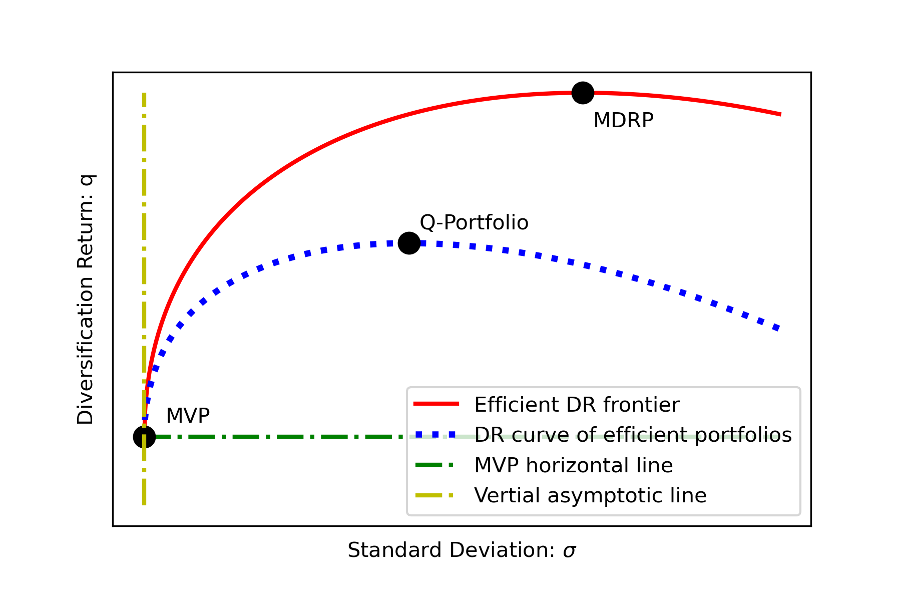
(a)

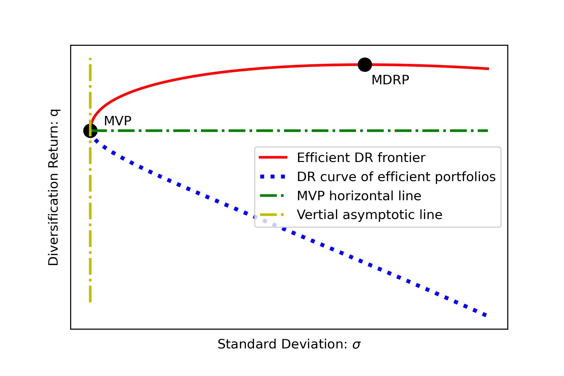
(b)

Figure 3: Graphical representation of the efficient DR frontier in the $(\sigma,q)$ space. Fig. 3(a) is for the case when $\eta^{\top}{\bf w}_{o}\geq 0$. The Q-portfolio is on the curve of the efficient portfolios and has the highest diversification return. It is below and on the left of MDRP. Fig. 3(b) is for $\eta^{\top}{\bf w}_{o}<0$. The efficient portfolio that has the highest diversification return is MVP. In both figures, the efficient DR frontier dominates the DR curve of MV efficient portfolios.

4.3 Comparison when there is a risk-free asset

Our study above can be straightforwardly extended to the important case when there is a risk-free asset. The classical Markowitz theory says the efficient portfolios form the Capital Market Line (CML) [30, 11]. We investigate how CML would look like on the $(\sigma,q)$ diagram. It turns out that it is a parabola with some nice features.

Suppose the risk-free asset has a return $r_{0}$ and it is treated as the $(n+1)$th assets, appended to the $n$ risky assets studied above. Let ${\bf w}_{T}$ denote the tangential portfolio (also known as the market portfolio). Then it is known (see e.g., [2, Section 5.2]):

$${\bf w}_{T}=\frac{1}{b-r_{0}a}V^{-1}\Big{(}\overline{{\bf r}}-r_{0}{\bf 1}_{n}\Big{)},$$

where the quantities $a$ and $b$ are defined in (25). For the tangential portfolio ${\bf w}_{T}$ to exist, the expected return of the minimum variance portfolio ${\bf w}_{\mbox{mvp}}$ must be greater than the risk-free asset return $r_{0}$, see [22]. This is equivalent to require $(b-r_{0}a)>0$.

Let

$$\Pi_{T}:=\left(\begin{array}[]{c}{\bf w}_{T}\\ 0\end{array}\right)\qquad\mbox{and}\qquad\Pi_{0}:=\left(\begin{array}[]{c}0\\ 1\end{array}\right)$$

be the respective representation of the tangential portfolio and the risk-free asset in the $(n+1)$ assets space. The portfolios on the CML can then be represented as

$$\Pi(\beta)=\Pi_{0}+\beta(\Pi_{T}-\Pi_{0}),\quad\beta\geq 0.$$

Let $\widetilde{V}$ denote the covariance matrix of the $(n+1)$ assets and $\widetilde{D}$ be the corresponding Euclidean distance matrix. We have

$$\widetilde{V}=\left[\begin{array}[]{cc}V&0\\ 0&0\end{array}\right]\quad\mbox{and}\quad\widetilde{D}=\left[\begin{array}[]{cc}D&\frac{1}{2}\eta\\[2.58334pt] \frac{1}{2}\eta^{\top}&0\end{array}\right]=\left[\begin{array}[]{cc}\frac{1}{2}(\eta{\bf 1}_{n}^{\top}+{\bf 1}_{n}\eta^{\top})-V&\frac{1}{2}\eta\\[2.58334pt] \frac{1}{2}\eta^{\top}&0\end{array}\right].$$

We compute the DR of the portfolio $\Pi$ using ${\bf 1}_{n}^{\top}{\bf w}_{T}=1$

$$q(\Pi) = \frac{1}{2}\Pi^{\top}\widetilde{D}\Pi$$ (31)

$$= -\frac{1}{2}\beta^{2}{\bf w}_{T}^{\top}V{\bf w}_{T}+\frac{1}{2}\beta^{2}(\eta^{\top}{\bf w}_{T})+\frac{1}{2}\beta(1-\beta)(\eta^{\top}{\bf w}_{T})$$

$$= -\frac{1}{2}\beta^{2}\sigma_{T}^{2}+\frac{1}{2}\beta(\eta^{\top}{\bf w}_{T}),$$

where $\sigma^{2}_{T}$ is the variance of the portfolio ${\bf w}_{T}$. On the other hand, the variance of the portfolio $\Pi$ is a quadratic function of $\beta$:

$$\sigma^{2}_{\Pi}=\beta^{2}\sigma^{2}_{T}.$$

Substituting it into (31), we get

$$q(\Pi)=-\frac{1}{2}\sigma^{2}_{\Pi}+\frac{\eta^{\top}{\bf w}_{T}}{2\sigma_{T}}\sigma_{\Pi}.$$

To indicate its dependence on CML, we denote $q(\Pi)$ by $q_{\mbox{cml}}(\sigma)$. Therefore, we have

$$q_{\mbox{cml}}(\sigma)=-\frac{1}{2}\sigma^{2}+\frac{\eta^{\top}{\bf w}_{T}}{2\sigma_{T}}\sigma=-\frac{1}{2}\left(\sigma-\frac{\eta^{\top}{\bf w}_{T}}{2\sigma_{T}}\right)^{2}+\frac{1}{8}\left(\frac{\eta^{\top}{\bf w}_{T}}{\sigma_{T}}\right)^{2}.$$ (32)

When $\eta^{\top}{\bf w}_{T}>0$, the largest DR portfolio happens at

$$\sigma=\frac{\eta^{\top}{\bf w}_{T}}{2\sigma_{T}}\qquad\mbox{or equivalently at}\qquad\beta=\frac{\eta^{\top}{\bf w}_{T}}{2\sigma^{2}_{T}}.$$

Having computed the DR curve (32) of the CML, we now compute the efficient DR curve for the $(n+1)$ assets. We note that we cannot directly apply the formula (13)) here for the following reasons: (i) there are $(n+1)$ assets here while $q_{\mbox{dr}}$ has only $n$ risky assets, and the DR of a portfolio depends on how many assets it has, see the discussion in Subsection 2.1; and (ii) the covariance matrix $V$ for $q_{\mbox{dr}}$ is assumed nonsingular, while $\widetilde{V}$ is singular. Hence, we need to compute the efficient DR curve from a scratch. Define

$$\widetilde{{\bf w}}(\sigma):=\arg\max\;\widetilde{q}(\widetilde{{\bf w}})=\frac{1}{2}\widetilde{{\bf w}}^{\top}\widetilde{D}\widetilde{{\bf w}},\ \mbox{s.t.}\ \left\{\begin{array}[]{l}{\bf 1}_{n+1}^{\top}\widetilde{{\bf w}}=1\\ {\bf w}^{\top}V{\bf w}=\sigma^{2}\end{array}\right.\quad\mbox{with}\quad\widetilde{{\bf w}}:=\left(\begin{array}[]{c}{\bf w}\\ w_{0}\end{array}\right)\in\Re^{n+1}$$ (33)

where $\sigma^{2}$ is a given level of the risk and $w_{0}$ represents the weight invested in the risk-free asset.

Using the fact that ${\bf 1}_{n}^{\top}{\bf w}=1-w_{0}$, we get $\widetilde{q}(\widetilde{{\bf w}})=q({\bf w}).$ Therefore, Problem (33) is equivalent to the following problem:

$$\widehat{{\bf w}}(\sigma):=\arg\max\;q({\bf w}),\quad\mbox{s.t.}\quad{\bf w}^{\top}V{\bf w}=\sigma^{2}.$$ (34)

The weight vector $\widehat{{\bf w}}(\sigma)$ is the risky part of $\widetilde{{\bf w}}(\sigma)$ and $\widehat{w}_{0}:=1-{\bf 1}_{n}^{\top}\widehat{{\bf w}}(\sigma)$ is the weight invested in the risk-free asset. Hence, $\widetilde{q}(\widetilde{{\bf w}}(\sigma))=q(\widehat{{\bf w}}(\sigma)).$ Repeating the computational procedure for $q_{\mbox{dr}}$ that leads to (13), we can compute for $q(\widehat{{\bf w}}(\sigma))$, which is given below:

$$q(\widehat{{\bf w}}(\sigma))=-\frac{1}{2}\sigma^{2}+\frac{\sigma}{2}\sqrt{\eta^{\top}V^{-1}\eta}=:\widetilde{q}_{\mbox{dr}}(\sigma),$$ (35)

where the optimal DR is denoted by $\widetilde{q}_{\mbox{dr}}(\sigma)$ to indicates it is the optimal DR under the given level of risk $\sigma^{2}$. This is the efficient DR curve for the $(n+1)$ assets. Comparison of (35) with (32) leads to the following two remarks.

• Both curves $\widetilde{q}_{\mbox{dr}}(\sigma)$ and $q_{\mbox{cml}}(\sigma)$ are of standard parabolas, and are much simpler than their counterparts $q_{\mbox{dr}}(\sigma)$ and $q_{\mbox{ef}}(\sigma)$ where only risky assets are considered. The fact that $\widetilde{q}_{\mbox{dr}}(\sigma)\geq q_{\mbox{cml}}(\sigma)$ (the efficient DR curve dominates the DR curve of CML) yields

  $$\sqrt{\eta^{\top}V^{-1}\eta}\sigma_{T}\geq\eta^{\top}{\bf w}_{T}.$$ (36)

  We further note that the quantity $(\eta^{\top}V^{-1}\eta)$ is $1/\sigma^{2}_{\eta}$ defined by

  $$\sigma^{2}_{\eta}:=\min{\bf w}^{\top}V{\bf w},\qquad\mbox{s.t.}\quad\eta^{\top}{\bf w}=1.$$

  Hence,the inequality (36) becomes

  $$\frac{\sigma_{T}}{\sigma_{\eta}}\geq\eta^{\top}{\bf w}_{T}.$$

  This inequality on the tangential portfolio ${\bf w}_{T}$ is new.

• When the variance vector $\eta$ is proportional to the excess rate of return $(\overline{{\bf r}}-r_{0}{\bf 1}_{n})$, i.e., $\eta=\gamma(\overline{{\bf r}}-r_{0}{\bf 1}_{n})$ for some $\gamma>0$, then we can prove $q_{\mbox{cml}}(\sigma)=\widetilde{q}(\sigma)$. In other words, the DR curve of CML becomes the efficient DR portfolio. This result generalizes Thm. 9(iv) to the case a risk-free asset is included. Otherwise, the gap can be measured as follows:

  $$\widetilde{q}(\sigma)-q_{\mbox{cml}}(\sigma)=\frac{\sigma}{2}\Big{(}\sqrt{\eta^{\top}V^{-1}\eta}-\frac{\eta^{\top}{\bf w}_{T}}{\sigma_{T}}\Big{)}\qquad\forall\ \sigma\geq 0.$$

  The gap is a linear function of $\sigma$. The curves of $q_{\mbox{cml}}(\sigma)$ and $\widetilde{q}(\sigma)$ are similar to their counterparts in Fig. 3.

5 A Numerical Illustration

Theoretically, we are largely clear what to expect of the diversification return based portfolios. In this part, we illustrate the behaviour of those portfolios using a real data set and compare them with some existing portfolios. The illustration reveals some interesting observations and enhances our understanding of those portfolios. In particular, we demonstrate the following:

• We illustrate the concerned portfolios in three graphs: $(\sigma,q)$ (standard deviation and diversification return) graph; $(\sigma,c)$ (standard deviation and centrality) graph; and $(\sigma,R)$ (standard deviation and return) graph.

• We also single out some particular portfolios. They include: MVP: Minimum Variance Portfolio; MDRP: Maximum Diversification Return Portfolio; $Q$-portfolio: the efficient mean-variance portfolio that has the largest diversification return; and MDP: Maximum Diversification ratio Portfolio, studied in [6]. This portfolio is explained below.

5.1 Maximum diversification ratio portfolio

Researchers often get confused between the Maximum Diversification Return Portfolio (MDRP) and the Maximum Diversification ratio Portfolio (MDP), which was initially studied by Choueifaty and Coignard [6]:

$${\bf w}_{\mbox{mdp}}:=\arg\max\;\frac{\sqrt{\eta}^{\top}{\bf w}}{\sqrt{{\bf w}^{\top}V{\bf w}}},\quad\mbox{s.t.}\quad{\bf 1}_{n}^{\top}{\bf w}=1.$$ (37)

It would be interesting to study their relationship. Obviously, (37) is equivalent to

$${\bf w}_{\mbox{mdp}}=\arg\max\;\left(\frac{\sqrt{\eta}^{\top}{\bf w}}{\sqrt{{\bf w}^{\top}V{\bf w}}}\right)^{2}=\frac{{\bf w}^{\top}\sqrt{\eta}\sqrt{\eta}^{\top}{\bf w}}{{\bf w}^{\top}V{\bf w}}\quad\mbox{s.t.}\quad{\bf 1}_{n}^{\top}{\bf w}=1.$$

Let us fixed the risk level at ${\bf w}^{\top}V{\bf w}=\sigma^{2}$ and consider the corresponding maximum diversification ratio portfolio:

$${\bf w}_{\mbox{mdp}}(\sigma):=\arg\max\;\frac{1}{2}{\bf w}^{\top}\sqrt{\eta}\sqrt{\eta}^{\top}{\bf w},\quad\mbox{s.t.}\quad{\bf 1}_{n}^{\top}{\bf w}=1,\ \ {\bf w}^{\top}V{\bf w}=\sigma^{2}.$$ (38)

We estimate the difference of the objectives of the two portfolios MDRP (10) and MDP (38):

$$d_{\sigma} := \frac{1}{2}\max_{{\bf w}}\;\eta^{\top}{\bf w}-\frac{1}{2}\max_{{\bf w}}\;{\bf w}^{\top}\sqrt{\eta}\sqrt{\eta}^{\top}{\bf w}$$

$$\leq \frac{1}{2}\max_{{\bf w}}\;\Big{(}\eta^{\top}{\bf w}-{\bf w}^{\top}\sqrt{\eta}\sqrt{\eta}^{\top}{\bf w}\Big{)}$$

$$= \frac{1}{2}\max_{{\bf w}}{\bf w}^{\top}\underbrace{\Big{(}\frac{1}{2}(\eta^{\top}{\bf 1}_{n}+{\bf 1}_{n}\eta^{\top})-\sqrt{\eta}\sqrt{\eta}^{\top}\Big{)}}_{=:D_{\eta}}{\bf w}$$

It is easy to see that

$$\mbox{diag}(D_{\eta})=0\quad\mbox{and}\quad-JD_{\eta}J=J\sqrt{\eta}\sqrt{\eta}^{\top}J\succeq 0,$$

where $J:=I_{n}-\frac{1}{n}{\bf 1}_{n}{\bf 1}_{n}^{\top}$ is the centering matrix. It follows from [16] (see also [24, Eq.(1)]) that $D_{\eta}$ is Euclidean distance matrix. Let us restrict to the long-only portfolio ${\bf w}\geq 0$ and define

$$S_{\sigma}^{+}:=\left\{{\bf w}\;|\;{\bf 1}_{n}^{\top}{\bf w}=1,\ \ {\bf w}^{\top}V{\bf w}=\sigma^{2},\ \ {\bf w}\geq 0\right\}.$$

On one hand,

$$-2d_{\sigma}=\max_{{\bf w}\in S_{\sigma}^{+}}\;{\bf w}^{\top}\sqrt{\eta}\sqrt{\eta}^{\top}{\bf w}-\max_{{\bf w}\in S_{\sigma}^{+}}\;\eta^{\top}{\bf w}\leq\max_{{\bf w}\in S_{\sigma}^{+}}{\bf w}^{\top}(-D_{\eta}){\bf w}\leq 0,$$

where the last inequality used the facts that $D_{\eta}$ is EDM (hence its elements are non-negative) and ${\bf w}\geq 0$. On the other hand,

$$d_{\sigma}\leq\left\{\max_{{\bf w}\geq 0}\frac{1}{2}{\bf w}^{\top}D_{\eta}{\bf w},\quad\mbox{s.t.}\quad{\bf 1}_{n}^{\top}{\bf w}=1\right\}=:d_{\max}.$$ (39)

Hence, for long-only portfolios (see [25]), we must have

$$\max_{{\bf w}\in S_{\sigma}^{+}}\;{\bf w}^{\top}\sqrt{\eta}\sqrt{\eta}^{\top}{\bf w}\leq\max_{{\bf w}\in S_{\sigma}^{+}}\;\eta^{\top}{\bf w}\leq\max_{{\bf w}\in S_{\sigma}^{+}}\;{\bf w}^{\top}\sqrt{\eta}\sqrt{\eta}^{\top}{\bf w}+d_{\max}.$$

We note that $d_{\max}>0$ is independent of the level of $\sigma^{2}$ of the portfolios involved. This means that, given any risk level $\sigma^{2}$, the distance between the two portfolios objectives is uniformly bounded irrelevant to the risk level. In other words, the diversification ratio portfolios should follow the trend of the diversification return portfolios. This is exactly what is observed in the following numerical example.

5.2 Dax30 data

This data set consists of $30$ stocks that have appeared in DAX30 Index (DAX30) and was used in [18, Page 336]. The data period is from January 3, 2017 to December 31, 2021. The mean and the covariance matrix of the daily returns were annualized. The averaged weekly data was also tested and the behaviours of the concerned portfolios are similar to that of the plotted graphs in Fig. 4, Fig. 5, and Fig. 6, and hence are omitted. In all three figures, we plots the portfolios of ${\bf w}_{\mbox{mdrp}}(\sigma)$ in (11), ${\bf w}_{\mbox{mv}}(\sigma)$ in (24) and ${\bf w}_{\mbox{mdp}}(\sigma)$ in (38) as $\sigma$ varies. They respectively represent the optimal diversification return portfolios, the optimal mean-variance portfolios, and the diversification return ratio portfolios. We note that only ${\bf w}_{\mbox{mv}}(\sigma)$ is explicitly related to the stock returns and the other two are only relevant to the covariances of the stocks.

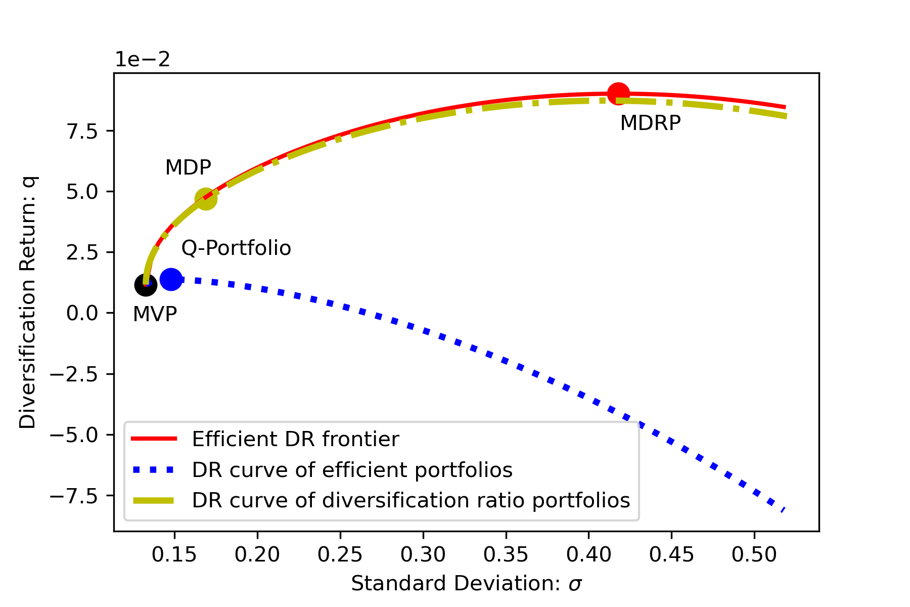
Figure 4: Comparison of portfolios in the $(\sigma,q)$ plane.

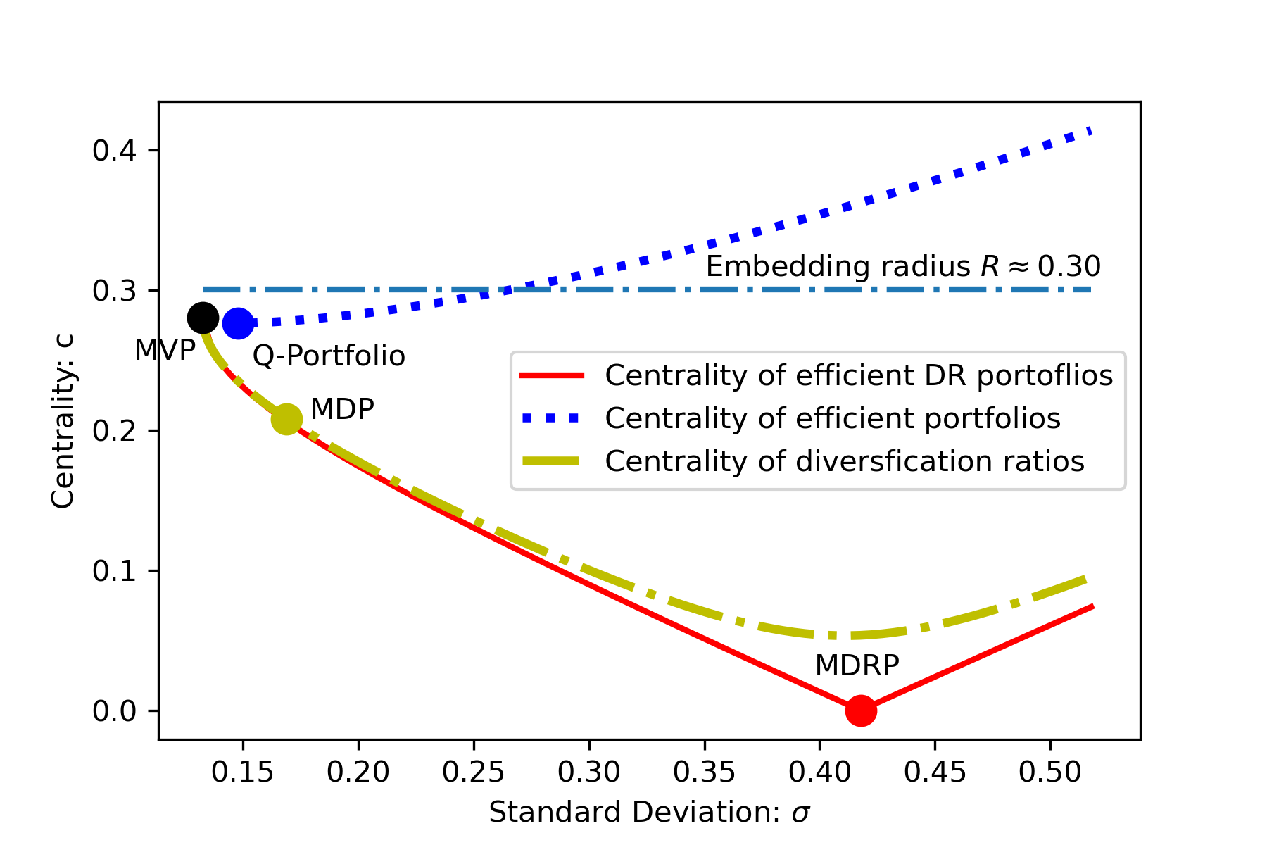
Figure 5: Comparison of portfolios in the $(\sigma,c)$ plane.

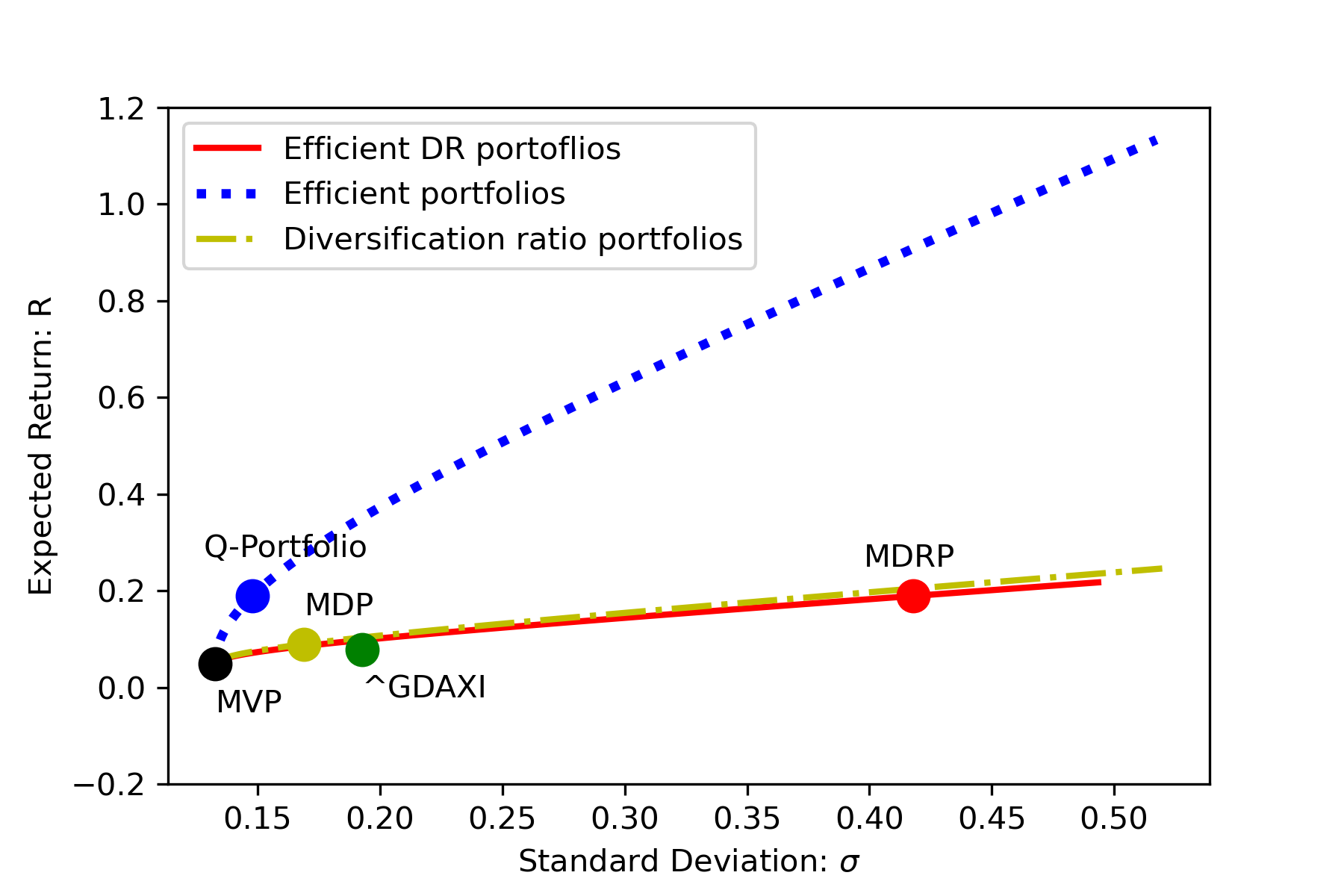
Figure 6: Comparison of portfolios in the $(\sigma,R)$ plane.

We summarized the key observations as follows.

• The efficient DR curve of the optimal diversification return portfolio ${\bf w}_{\mbox{mdrp}}(\sigma)$ and that of the optimal diversification ratio portfolio ${\bf w}_{\mbox{mdp}}(\sigma)$ are surprisingly close, see the standard-deviation and diversification-return $(\sigma,q)$ graph in Fig. 4. It is partially because their respective objectives are not far from each other and the gap is uniformly bounded irrelevant of the risk level involved. Equally surprising is their similar expected returns, as shown in the standard-deviation and return $(\sigma,R)$ graph in Fig. 6. However, their difference was vivid in the standard-deviation and centrality $(\sigma,c)$ graph in Fig. 5. It seems that the centrality curve of MDP is smoother than that of MDRP. Furthermore, the centrality of ${\bf w}_{\mbox{mdp}}(\sigma)$ is strictly above that of ${\bf w}_{\mbox{mdrp}}(\sigma)$. However, a general trend is that they follow each other.

• Contrary to the observation above, the trajectory of the mean-variance portfolio goes the opposite way to that of MDRP and MDP. In particular, the diversification return of efficient MV portfolios quickly went negative, see Fig. 4. This means as the standard deviation $\sigma$ (equivalently, the expected return) is above a certain threshold, they tend to concentrate on few assets leading to less diversified portfolios. This is also reflected on the centrality graph Fig. 5. Any MV portfolios that are above the horizontal line corresponding to the embedding radius $R\approx 0.30$ has negative $q$ according to the formula (5). Another drawback of MV portfolios for this dataset is that its expected return grows too fast, see Fig. 6. We also plotted the Dax index return itself, denoted as ^∧GDAXI (the tick symbol of the index), which is very close to the return curve of efficient diversification return portfolios, and is far below the efficient frontier.

• There is a clear cluster among the interested portfolios. The portfolios of MVP, MDP and Q-portfolio form a cluster in all three figures. Moreover, the market portfolio ^∧GDAXI is also close to this cluster, meaning that portfolios near this cluster tends to follows the market trend. More numerical experiments are needed to see if it is a universal observation. Although the efficient portfolios tend to quickly yield negative DR, the Q-portfolio has positive DR and should be numerically investigated to validate its value. In contrast, MDRP is far away from the cluster. The return of the efficient DR portfolios in Fig. 6 looks flat and this indicates that the increase in return is much slower than that of the standard deviation. This observation confirms once again that MDRP and MDP are based on two very different criteria though they both stay close to one curve in each of the plots.

6 Conclusion

This paper provided a thorough study of the diversification return based portfolio from an optimization perspective. It shows that there is intrinsic connection between the diversification return and the norm-weighted portfolio, and a separation theorem also holds for the efficient diversification return portfolios. The DR curve of those portfolio is strongly concave in the $(\sigma,q)$ space. Consequently, any portfolio beyond MDRP is discarded as it would have higher standard deviation than MDRP, but with less DR. The separation theorem implies that the meaningful portfolios are convex combination of MVP and MDRP. We also derived a formula for the DR curve of the mean-variance efficient portfolios and conducted its comparison with the efficient DR curve. In particular, the Q-portfolio seems to have some advantages than other MV efficient portfolio. We also extend such investigation to the case where a risk free asset is also available. The DR curves for this case are standard parabolas and the risk adjusted gap between the two DR curves is constant. We also investigated the link between MDRP and the maximum diversification ratio portfolio (MDP). Although they are based on different criterion, they tend to follow each other and this is well demonstrated in the numerical example.

The good understanding of the DR portfolios also prompts an important question: how to enhance the DR model under noisy environment. This would naturally lead to robust variants, that have been widely studied for the MV models, see [5, 12]. We plan to investigate this possibility in our next research.

References

- [1] David G Booth and Eugene F Fama. Diversification returns and asset contributions. Financial Analysts Journal, 48(3):26–32, 1992.
- [2] Pierre Brugière. Quantitative portfolio management. Springer Texts in Business and Economics, 2020.
- [3] Benoît Carmichael, Gilles Boevi Koumou, and Kevin Moran. Rao’s quadratic entropy and maximum diversification indexation. Quantitative Finance, 18(6):1017–1031, 2018.
- [4] Donald R Chambers and John S Zdanowicz. The limitations of diversification return. The Journa of Portfolio Management, 40(4):65–76, 2014.
- [5] Li Chen, Simai He, and Shuzhong Zhang. Tight bounds for some risk measures, with applications to robust portfolio selection. Operations Research, 59(4):847–865, 2011.
- [6] Yves Choueifaty and Yves Coignard. Toward maximum diversification. The Journal of Portfolio Management, 35(1):40–51, 2008.
- [7] Keith Cuthbertson, Simon Hayley, Nick Motson, and Dirk Nitzsche. Diversification returns, rebalancing returns and volatility pumping. Rebalancing Returns and Volatility Pumping (January 14, 2015), 2015.
- [8] Victor DeMiguel, Lorenzo Garlappi, Francisco J Nogales, and Raman Uppal. A generalized approach to portfolio optimization: Improving performance by constraining portfolio norms. Management science, 55(5):798–812, 2009.
- [9] Edwin J Elton, Martin J Gruber, Stephen J Brown, and William N Goetzmann. Modern portfolio theory and investment analysis. John Wiley & Sons, 2009.
- [10] Claude B Erb and Campbell R Harvey. The strategic and tactical value of commodity futures. Financial Analysts Journal, 62(2):69–97, 2006.
- [11] Eugene F Fama and Kenneth R French. The capital asset pricing model: Theory and evidence. Journal of economic perspectives, 18(3):25–46, 2004.
- [12] Alireza Ghahtarani, Ahmed Saif, and Alireza Ghasemi. Robust portfolio selection problems: a comprehensive review. Operational Research, 22(4):3203–3264, 2022.
- [13] Jun-ya Gotoh and Akiko Takeda. On the role of norm constraints in portfolio selection. Computational Management Science, 8(4):323–353, 2011.
- [14] John C Gower. Some distance properties of latent root and vector methods used in multivariate analysis. Biometrika, 53(3-4):325–338, 1966.
- [15] John Clifford Gower. Euclidean distance geometry. Math. Sci., 1:1–14, 1982.
- [16] John Clifford Gower. Properties of euclidean and non-euclidean distance matrices. Linear algebra and its applications, 67:81–97, 1985.
- [17] Jason T Greene and David A Rakowski. The sources of portfolio returns: Underlying stock returns and the excess growth rate. Available at SSRN 1802591, 2011.
- [18] Yves Hilpisch. Python for Finance: Analyze big financial data. ” O’Reilly Media, Inc.”, 2014.
- [19] Ravi Jagannathan and Tongshu Ma. Risk reduction in large portfolios: Why imposing the wrong constraints helps. The Journal of Finance, 58(4):1651–1683, 2003.
- [20] Sergiy Lesyk and Andrew Dougan. The role of diversification return in factor portfolios. ftserussell.com, 2021.
- [21] Jean-Michel Maeso and Lionel Martellini. Maximizing an equity portfolio excess growth rate: a new form of smart beta strategy? Quantitative Finance, 20(7):1185–1197, 2020.
- [22] Robert C Merton. An analytic derivation of the efficient portfolio frontier. Journal of financial and quantitative analysis, 7(4):1851–1872, 1972.
- [23] Frieder Meyer-Bullerdiek. Rebalancing and diversification return–evidence from the german stock market. Journal of Finance and Investment Analysis, 6(2):1–28, 2017.
- [24] Hou-Duo Qi. A semismooth newton method for the nearest euclidean distance matrix problem. SIAM Journal on Matrix analysis and applications, 34(1):67–93, 2013.
- [25] Hou-Duo Qi. On the long-only minimum variance portfolio under single factor model. Operations Research Letters, 49(5):795–801, 2021.
- [26] Hou-Duo Qi. Geometric characterization of maximum diversification return portfolio via rao’s quadartic entropy. SIAM Journal on Financial Mathematics (to appear), 2023.
- [27] Edward Qian. Diversification return and leveraged portfolios. The Journal of Portfolio Management, 38(4):14–25, 2012.
- [28] C Radhakrishna Rao. Diversity: Its measurement, decomposition, apportionment and analysis. Sankhyā: The Indian Journal of Statistics, Series A, 44(1):1–22, 1982.
- [29] IJ Schoenberg. Remarks to maurice frechet’s article” sur la definition axiomatique d’une classe d’espace distancies vector-! ellement applicable sur l’espace de hilbertl. Ann. of Math, 36:724–732, 1935.
- [30] William F Sharpe. Capital asset prices: A theory of market equilibrium under conditions of risk. The journal of finance, 19(3):425–442, 1964.
- [31] James Tobin. Liquidity preference as behavior towards risk. The review of economic studies, 25(2):65–86, 1958.
- [32] Scott Willenbrock. Diversification return, portfolio rebalancing, and the commodity return puzzle. Financial Analysts Journal, 67(4):42–49, 2011.
- [33] Yu-Min Yen and Tso-Jung Yen. Solving norm constrained portfolio optimization via coordinate-wise descent algorithms. Computational Statistics & Data Analysis, 76:737–759, 2014.
- [34] Gale Young and Aiston S Householder. Discussion of a set of points in terms of their mutual distances. Psychometrika, 3(1):19–22, 1938.
- [35] Hongxin Zhao, Lingchen Kong, and Hou-Duo Qi. Optimal portfolio selections vian -norm regularization. Computational Optimization and Applications, 80(3):853–881, 2021.