Multimass modelling of Milky Way globular clusters - I. Implications on their stellar initial mass function above $1\ \mathrm{M}_{\odot}$

Abstract

The distribution of stars and stellar remnants (white dwarfs, neutron stars, black holes) within globular clusters holds clues about their formation and long-term evolution, with important implications for their initial mass function (IMF) and the formation of black hole mergers. In this work, we present best-fitting multimass models for 37 Milky Way globular clusters, which were inferred from various datasets, including proper motions from Gaia EDR3 and HST, line-of-sight velocities from ground-based spectroscopy and deep stellar mass functions from HST. We use metallicity dependent stellar evolution recipes to obtain present-day mass functions of stars and remnants from the IMF. By dynamically probing the present-day mass function of all objects in a cluster, including the mass distribution of remnants, these models allow us to explore in detail the stellar (initial) mass functions of a large sample of Milky Way GCs. We show that, while the low-mass mass function slopes are strongly dependent on the dynamical age of the clusters, the high-mass slope ($\alpha_{3};m>$1\text{\,}\mathrm{M}_{\odot}$$) is not, indicating that the mass function in this regime has generally been less affected by dynamical mass loss. Examination of this high-mass mass function slope suggests an IMF in this mass regime consistent with a Salpeter IMF is required to reproduce the observations. This high-mass IMF is incompatible with a top-heavy IMF, as has been proposed recently. Finally, based on multimass model fits to our sample of Milky Way GCs, no significant correlation is found between the high-mass IMF slope and cluster metallicity.

1 Introduction

The stellar initial mass function (IMF) plays a key role in the evolutionary history and properties of populations of stars, and understanding it is vital to understanding and interpreting both observations and simulations of star clusters and galaxies.

Globular clusters (GCs) consist of very large numbers of stars of similar iron abundance and age, providing us with one of the best avenues for investigating the shape of the stellar IMF, and how it may vary with environment. The IMF plays a particularly important role in the evolution of GCs, where it controls the populations of stellar remnants, the degree and timescale of mass segregation, the lifetime of the clusters before dissolution, and the contribution of GCs to observed gravitational waves (e.g. Haghi et al., 2020; Weatherford et al., 2021; Wang et al., 2021).

The universality of the stellar IMF is a debated topic. While the typically assumed (canonical) formulations of the IMF, determined empirically through observations of solar-neighbourhood and Milky Way cluster stars (e.g. Salpeter, 1955; Kroupa, 2001; Chabrier, 2003), seem to demonstrate that it is universal among star-forming systems, the exact shape and universality of the IMF is still under investigation (see review by Bastian et al., 2010). For example, observations of the cores of early-type galaxies, (both spectroscopic; van Dokkum & Conroy, 2010 and kinematic; Cappellari et al., 2012) have pointed towards a “bottom-heavy” IMF, enriched with low-mass stars, in those environments (although see also Smith, 2014, 2020). Meanwhile, recent theoretical studies of star and cluster formation have indicated that certain environment-dependent processes, such as radiative feedback or cooling from dust-grains, could imply a varying IMF (Krumholz et al., 2011; Chon et al., 2021).

In particular for GCs, some recent observational works have also showcased trends which could be explained by a varying IMF. These observations, however, have also been shown to be explainable without the need to invoke such a non-canonical IMF. Strader et al. (2011) demonstrated that dynamical mass measurements of 200 globular clusters in M 31 showed a decreasing trend in the dynamical mass-to-light ratio with increasing cluster metallicity. This result is opposite to what standard stellar population models would predict while assuming a canonical IMF. Haghi et al. (2017) showed that these results could be explained by introducing a non-canonical, metallicity-dependent IMF, with an increasing level of top-heaviness for low metallicity clusters (Marks et al., 2012). However Baumgardt et al. (2020), in a study of Milky Way GCs, also noted that such a discrepancy in the mass-to-light ratios compared to population synthesis models could be accounted for once the low-mass depleted present-day mass function (PDMF) of the metal-rich clusters was taken into consideration. Metallicity-dependent stellar evolution models were also able to account for the difference in the metal-poor clusters. Shanahan & Gieles (2015) also demonstrated that not accounting for mass segregation in integrated-light studies of M 31 clusters introduces a bias in the inferred dynamical mass, dependent on metallicity (see also Sippel et al., 2012), and argued that there is no need for variations in the IMF to explain the Strader et al. results. Because the majority of stars form in GCs at low metallicities (Larsen et al., 2012), a substantially flatter IMF at high masses in GCs would have important consequences for the amount of ionization radiation at high redshift (Schaerer & Charbonnel, 2011; Boylan-Kolchin, 2018); the chemical evolution of galaxies; the amount of stellar-mass black holes (BHs) formed and subsequent binary BH mergers (Schneider et al., 2018). A flat IMF also predicts that there should be more white dwarfs (WDs) at the present age. WDs contribute $\sim 30\%$ to the total mass at $\sim 10\,\mathrm{Gyr}$ for a canonical IMF, before accounting for the preferential loss of low-mass objects in GCs. The fractional contribution to the central density is higher because of mass segregation, so it is feasible to look for an excess of WDs in the kinematics of GCs.

In this work, the hypothesis of metallicity-dependent, variable and non-canonical stellar IMFs in globular clusters is investigated, in particular in the high-mass regime, where stars in old globular clusters have, by the present day, evolved into stellar remnants. To do so, we fit multimass dynamical models to various observables for a large sample of Milky Way clusters, over a range of metallicities. We infer their global stellar mass functions and simultaneously constrain their distributions of stellar remnants. The multimass limepy models and mass function evolution algorithm used are explained in more detail in Section 2. Section 3 describes the methods and sources used to obtain all observational data used to fit the models, as well as how the cluster sample was chosen. The model fitting procedure, including descriptions of all probability distributions and Bayesian sampling techniques, as well as the software library and fitting pipeline which was created to facilitate this fitting, is presented in Section 4. The results of the fitting of all clusters in our sample based on these methods are given in Section 5. The (initial) mass function results for all clusters are presented and explored in more detail in Section 6. Finally, we conclude in Section 7.

The inferred present-day populations of stellar-mass BHs in our sample of globular clusters based on our best-fitting models will be examined in detail in a separate paper (Dickson et al., in prep.; hereafter Paper II).

2 Models

To model the mass distribution of the globular clusters analyzed in this work, we use the limepy multimass distribution-function (DF) based models (Gieles & Zocchi, 2015) . DF based models are equilibrium models built around a distribution function $f$ which describes the particle density of stars and satisfies the collisionless-Boltzmann equation. This DF is used to self-consistently solve for the system’s potential ($\phi(r)$) using Poisson’s equation.

A variety of quantities can be derived from the DF which can be used to describe a globular cluster, including the projected velocity dispersion (the second velocity moment), the projected surface density, the total mass, the potential energy and the system entropy (e.g. Spitzer, 1987; Gieles & Zocchi, 2015). Observational data can be used to compare and constrain the models based on these quantities.

Multimass models allow for a more accurate description of real globular clusters, which are made up of a spectrum of stellar masses. Multiple mass components are necessary in order to describe the distributions of different stellar and remnant populations within the system and, in turn, examine both the process and effects of mass segregation (e.g. Da Costa & Freeman, 1976).

The DF of the multimass version of the limepy models is given by the sum of component DFs for every mass bin $j$, each as a function of the specific energy $E$ and angular momentum $J$ in the form of:

$$f_{j}(E,J^{2})=\begin{dcases}A_{j}\,\exp\left(-\frac{J^{2}}{2r_{\mathrm{a},j}^{2}s_{j}^{2}}\right)\,E_{g}\left(-\frac{E-\phi(r_{\mathrm{t}})}{s_{j}^{2}}\right)&E<\phi(r_{t}),\\ 0&E\geq\phi(r_{t}),\end{dcases}$$ (1)

where $A_{j}$ and $s_{j}$ are the mass-dependant normalization and velocity scales, $r_{\mathrm{a},j}$and $r_{\mathrm{t}}$are the anisotropy and truncation radii, and the function $E_{g}$ is defined using the regularized lower incomplete gamma function and the truncation parameter $g$:

$$E_{g}(x)=\begin{dcases}\exp(x)&g=0,\\ \exp(x)\frac{\gamma(g,x)}{\Gamma(g)}&g>0,\end{dcases}$$ (2)

These parameters and how they are used are explained in more detail in Section 2.1 below.

2.1 Model parameters

Our models are defined by 10 free parameters (listed in Table 1) which dictate the mass function and physical solution of the limepy DF.

Parameter	Description	Prior
$\hat{\phi}_{0}$	Dimensionless central potential	$\mathrm{Uniform}(L=2.0,\ U=15.0)$
$M$	Total system mass $\left[10^{6}\ \mathrm{M}_{\odot}\right]$	$\mathrm{Uniform}(L=0.001,\ U=2.0)$
$g$	Truncation parameter	$\mathrm{Uniform}(L=0.0,\ U=3.5)^{\ast}$
$r_{\mathrm{h}}$	Half-mass radius $[\mathrm{pc}]$	$\mathrm{Uniform}(L=0.5,\ U=15.0)$
$\log(\hat{r}_{\mathrm{a}})$	Dimensionless anisotropy radius	$\mathrm{Uniform}(L=0.0,\ U=8.0)$
$\delta$	Velocity-scale mass dependence	$\mathrm{Uniform}(L=0.3,\ U=0.5)^{\ast}$
$\alpha_{1}$	MF exponent $(0.1\ \mathrm{M}_{\odot}<m\leq 0.5\ \mathrm{M}_{\odot})$	$\mathrm{Uniform}(L=-1.0,\ U=2.35)^{\ast}$
$\alpha_{2}$	MF exponent $(0.5\ \mathrm{M}_{\odot}<m\leq 1\ \mathrm{M}_{\odot})$	$\mathrm{Uniform}(L=-1.0,\ U=\mathrm{min}(2.35,\ \alpha_{1}))^{\ast}$
$\alpha_{3}$	MF exponent $(1\ \mathrm{M}_{\odot}<m\leq 100\ \mathrm{M}_{\odot})$	$\mathrm{Uniform}(L=1.6,\ U=\mathrm{min}(4.0,\ \alpha_{2}))^{\ast}$
$\mathrm{BH}_{\mathrm{ret}}$	Black hole retention fraction $[\%]$	$\mathrm{Uniform}(L=0.0,\ U=30.0)$
$F$	Mass function nuisance parameter	$\mathrm{Uniform}(L=1.0,\ U=7.5)$
$s^{2}$	Number density nuisance parameter $\left[\mathrm{arcmin}^{-4}\right]$	$\mathrm{Uniform}(L=0.0,\ U=15.0)$
$d$	Heliocentric distance $[\mathrm{kpc}]$	$\mathrm{Gaussian}(\mu=d_{\mathrm{lit}},\ \sigma=\delta d_{\mathrm{lit}})$

Table 1: List of all free parameters, their descriptions and the prior probability distributions used to bound their values. The first six are structural limepy parameters (Section 2.1), while the next four define the mass function (Section 2.2). The final three parameters aid in comparing models to observations (Section 4.1). The prior distributions shown here, when not motivated by physical or model constraints (marked here by an asterisk; see Section 4.1.2), are chosen to bound a large enough area of parameter space containing all valid parameter values. The bounds here represent the largest extents used. In reality, the bounds may be reduced slightly during the sampling of certain clusters in order to improve the performance of the sampler, while still including a large area surrounding the most likely parameter values. The literature values and uncertainties used in the prior on the distance are taken from Baumgardt & Vasiliev (2021).

The overall structure of these models is controlled by the (dimensionless) central potential parameter $\hat{\phi}_{0}$, which is used as a boundary condition for solving Poisson’s equation and defines how centrally concentrated the model is. The cluster model is spherical out to the truncation radius of the system, where its energy is reduced, mimicking the effects of the host galaxy’s tides, which reduce the escape velocity of stars, making it easier for them to escape. The sharpness of this energy truncation is defined by the truncation parameter $g$. Lower $g$ values result in a more abrupt energy truncation, increasing up to models with the maximum possible finite extent at $g=3.5$, while finite models with realistic values of $\hat{\phi}_{0}$ are typically limited to $g\lesssim 2.5$ (Gieles & Zocchi, 2015).

The mass and size scales of the model can be expressed in any desired physical units by adopting corresponding values for the normalization constant $A$ and the global velocity scale $s$. We opt to scale the models to match observations using the parameters for total cluster mass $M$ and 3D half-mass radius $r_{\mathrm{h}}$ as mass and size scales, which are used internally to compute the $A$ and $s$ scales.

limepy models allow for velocity anisotropy through an angular momentum term in the DF. With this term, the system is isotropic in the core, gains a degree of radial velocity anisotropy near the anisotropy radius $r_{\mathrm{a}}$, and then becomes isotropic once more near the truncation radius. This parametrization mimics how GCs naturally develop radially-biased velocity anisotropy throughout their evolution as a result of two-body relaxation and tides (Zocchi et al., 2016; Tiongco et al., 2016). The two-body relaxation process drives the core of clusters to isotropy, however scattering (on preferentially radial orbits) of stars outside the core acts to increase the radial component of the velocity dispersion. Finally, a combination of the tidal torque from the host galaxy, which induces a transfer of angular momentum near the Jacobi radius to stellar orbits in the tangential direction (Oh & Lin, 1992), and the preferential loss of stars on radial orbits (Tiongco et al., 2016), act to increase the tangentiality of the outer stars, damping the amount of radial anisotropy and leading to a return to isotropy near the immediate edge of the system. The anisotropy radius $r_{\mathrm{a}}$ dictates the amount of radial velocity anisotropy present in the models. The smaller the value of $r_{\mathrm{a}}$, the more anisotropic the system. In the limit $r_{\mathrm{a}}\to\infty$, the models become entirely isotropic. In practice, models with $r_{\mathrm{a}}$ greater than the cluster truncation radius can be considered isotropic.

The exact meaning of both the $\hat{\phi}_{0}$ and $\hat{r}_{\mathrm{a}}$ parameters depends on the definition of the mean mass (Peuten et al., 2017). In this work we adopt the global mean mass, that is, the mean mass of all stars in the entire cluster.

The multimass version of the limepy DF is defined by the sum of similar component DFs for each mass bin $j$, with mass-dependent velocity ($s_{j}$) and anisotropy radius ($r_{\mathrm{a},j}$) scales. The mass-dependent velocity scaling captures the trend towards kinetic energy equipartition among stars of different masses and models the effects of mass segregation (Gieles & Zocchi, 2015; Peuten et al., 2017; Hénault-Brunet et al., 2019). The velocity scale is defined based on the parameter $\delta$, such that $s_{j}\propto sm_{j}^{-\delta}$, where $s$ is defined as above. The mass-dependent anisotropy radius is defined in a similar fashion, using a parameter $\eta$ ($r_{\mathrm{a},j}\propto r_{\mathrm{a}}m_{j}^{\eta}$). For the analysis presented in this paper we have chosen to fix $\eta$ to 0, defining the anisotropy to be identical among all mass bins, the default assumption in multimass DF-based models. Our observations do not contain the information that would allow us to constrain the mass-dependence of the velocity anisotropy (e.g. Peuten et al., 2017), and thus the $\eta$ parameter.

Finally, the constituent discrete mass components which approximate the mass spectrum of a GC are represented in the multimass limepy models by the total ($M_{j}$) and mean ($m_{j}$) masses of each mass bin. These must be defined a priori by external methods, based on the mass function ($\alpha_{1},\alpha_{2},\alpha_{3}$) and BH retention percentage ($\mathrm{BH}_{\mathrm{ret}}$) parameters. The algorithm, which takes into account stellar evolution to predict the mean and total mass in stellar remnant bins, is described in detail in Section 2.2 below.

External to the limepy models themselves, we also employ a few extra parameters to aid in the fitting of the models to observations. These parameters are explained in more detail in Section 4.1.

2.2 Mass function evolution

DF-based models, such as limepy, compute the distribution of mass and velocity in a system in equilibrium. They are instantaneous “snapshot” models, and do not directly simulate any temporal astrophysical processes during their computation, including stellar evolution. As such, in order to determine the realistic mass populations for which the model will determine the phase-space distribution, we must incorporate a separate prescription for stellar evolution from an initial mass function, over the age of the cluster, to the present-day stellar and remnant mass functions.

In keeping with the formulation of canonical IMFs (e.g. Kroupa, 2001), we use a 3-component broken power law:

$$\xi(m)\propto\begin{dcases}m^{-\alpha_{1}}&0.1\ \mathrm{M}_{\odot}<m\leq 0.5\ \mathrm{M}_{\odot},\\ m^{-\alpha_{2}}&0.5\ \mathrm{M}_{\odot}<m\leq 1\ \mathrm{M}_{\odot},\\ m^{-\alpha_{3}}&1\ \mathrm{M}_{\odot}<m\leq 100\ \mathrm{M}_{\odot},\\ \end{dcases}$$ (3)

where the $\alpha_{i}$ parameters define the power-law ‘slope’ of each component, and are allowed to vary freely during model fitting, and $\xi(m)\differential{m}$ is the number of stars with masses within the interval $[m,\ m+\differential{m}]$. It should be noted here that our exact choices of break masses (0.1, 0.5, 1, 100 $\mathrm{M}_{\odot}$) are different than that of Kroupa (2001), to allow for a more specific study of the high-mass ($m>$1\text{\,}\mathrm{M}_{\odot}$$) regime.

To evolve the population of stars to the present day we follow the algorithm first described by Balbinot & Gieles (2018) and expanded upon in the ssptools library. This method is summarized below.

To begin, the rate of change of the number of main-sequence stars over time is given by the equation:

$$\dot{N}(m_{\mathrm{to}})=-\left.\derivative{N}{m}\right|_{m_{\mathrm{to}}}\left|\derivative{m_{\mathrm{to}}}{t}\right|,$$ (4)

where the amount of initial stars per unit mass ($\derivative*{N}{m}$) at the turn-off mass ($m_{\mathrm{to}}$) is given by the IMF, and the rate of change of the turn-off mass can be derived by approximating the lifetime of main-sequence stars as a function of initial mass:

$$t_{\mathrm{ms}}=a_{0}\exp(a_{1}m^{a_{2}}),$$ (5)

where the $a_{i}$ coefficients are interpolated from the Dartmouth Stellar Evolution Program models (Dotter et al., 2007; Dotter et al., 2008). This equation can then be inverted and differentiated to find the rate of change:

$$\derivative{m_{to}}{t}=\frac{1}{a_{1}a_{2}}\frac{1}{t}\left(\frac{\log(t/a_{0})}{a_{1}}\right)^{1/a_{2}-1}.$$ (6)

This set of equations dictates the amount of stars which evolve off the main sequence by the present-day cluster age $t$.

In this work we use 30 discrete stellar mass bins, each logarithmically-spaced within the bounds of the three components defined by the IMF (5 bins in the low and intermediate-mass regime and 20 bins in the high-mass regime) and 30 identically spaced remnant mass bins, which are filled by the remnants resulting from stars evolving off the main-sequence. As these stars evolve, the stellar remnants they will form (both in type and in mass), and thus the final remnant mass bins they will populate, depends on their initial mass and metallicity, and a functional initial-final mass relation (IFMR).

The WD IFMR is computed as a 10th order polynomial:

$$m_{\mathrm{WD}}=\sum_{j=0}^{10}b_{j}m_{i}^{j}$$ (7)

where $m_{i}$ is the initial mass of the star, $m_{\mathrm{WD}}$ is final mass of the formed remnant, and the coefficients $b_{j}$ and the maximum initial mass which will form a WD are interpolated, based on metallicity, from the MIST 2018 isochrones (Dotter, 2016; Choi et al., 2016).

The BH IFMR, as well as the minimum initial mass required to form a BH, is interpolated directly from a grid of stellar evolution library (SSE) models (Banerjee et al., 2020), using the rapid supernova scheme (Fryer et al., 2012), and is also dependent on metallicity. These relations are shown in Figure 1. All stars with initial masses between the WD and BH precursor masses are assumed to form neutron stars (NS). For simplicity, their final mass is always assumed to be $1.4\mathrm{M}_{\odot}$, regardless of the initial mass.

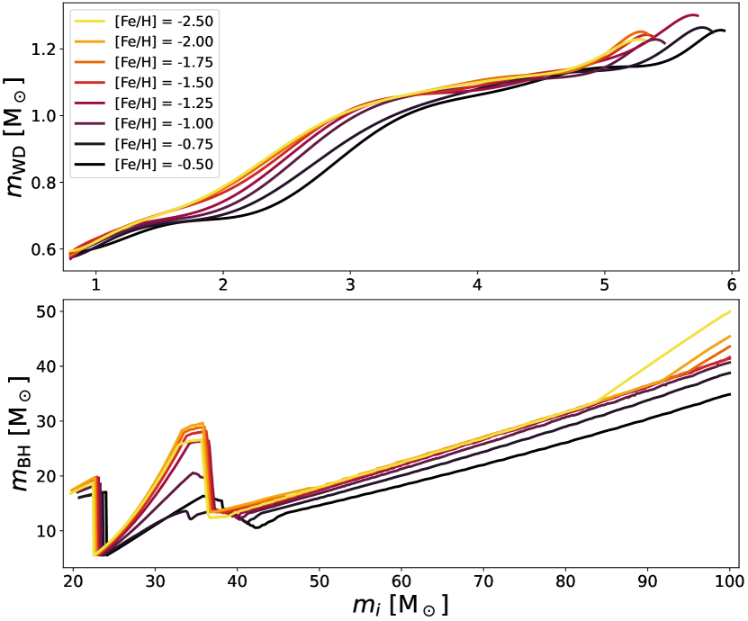
Figure 1: Adopted metallicity-dependent initial-final mass relations for white dwarf (top panel) and black hole (bottom panel) formation. Lower metallicities generally result in higher final remnant masses.

The amount and final mass of these remnants (as dictated by Equation 4) must then be scaled downwards by an “initial retention fraction” $f_{\mathrm{ret}}$, in order to mimic the loss of newly formed remnants due to natal kicks. For WDs we assume this is always equal to 100%. In this analysis, we assume a NS retention fraction of 10%, as is common (e.g. Pfahl et al., 2002), however, as shown in Hénault-Brunet et al. (2020), our results are insensitive to this exact value.

The mass function evolution algorithm includes two more specific prescriptions for the loss of BHs, accounting for dynamical ejections in addition to natal kicks.

Firstly the ejection of, primarily low-mass, BHs through natal kicks is simulated. We begin by assuming that the kick velocity is drawn from a Maxwellian distribution with a dispersion of $265\text{\,}\mathrm{km}\text{\,}{\mathrm{s}}^{-1}$, as has been found for neutron stars (Hobbs et al., 2005). This velocity is then scaled down linearly by the “fallback fraction” $f_{\mathrm{b}}$, the fraction of the precursor stellar envelope which falls back onto the BH after the initial supernova explosion. This fraction is interpolated from the same grid of SSE models used for the BH IFMR. The fraction of BHs retained in each mass bin is then found by integrating the Maxwellian kick velocity distribution from 0 to the system escape velocity. The initial system escape velocity of each cluster was estimated by assuming that about half of the initial cluster mass was lost through stellar evolution, while adiabatically expanding the cluster to a present-day half-mass radius a factor of two larger than the initial value, resulting in an initial escape velocity twice as large as the present-day value. A set of preliminary models were computed for all clusters, and the initial escape velocity was computed based on the best-fitting central density as $v_{\mathrm{esc}}=2\sqrt{-2\phi_{0}}$, where $\phi_{0}$ is the central potential. It should be noted that clusters with an escape velocity $\gtrsim$100\text{\,}\mathrm{km}\text{\,}{\mathrm{s}}^{-1}$$ will retain nearly all BHs (Antonini, Gieles & Gualandris, 2019).

Black holes are also ejected over time from the core of GCs due to dynamical interactions with one another (e.g. Breen & Heggie, 2013a, b). This process is simulated through the removal of BHs, beginning with the heaviest mass bins (with larger gravitational interaction cross-sections) through to the lightest (Morscher et al., 2015; Antonini & Gieles, 2020), until the combination of mass in BHs lost through both the natal kicks and these dynamical ejections leads to a retained mass in BHs corresponding to the percentage of the initial mass in BHs specified by the BH mass retention fraction parameter ($\mathrm{BH}_{\mathrm{ret}}$).

The final avenue for cluster mass loss is through the escape of stars and remnants driven by two-body relaxation and lost to the host galaxy. Such losses, in a mass segregated cluster, are dominated by the escape of low-mass objects from the outer regions of the cluster. Determining the overall losses through this process is a complicated task, dependent on the dynamical history and orbital evolution of the cluster, which we do not attempt to model here. We thus opt to ignore this preferential loss of low-mass stars and do not further model the escape of any stars, apart from through the processes described above. This means that the low-mass $\alpha$ exponents determined here may, in most cases, describe most accurately the PDMF rather than the low-mass IMF of our clusters. This is discussed in more detail in Section 6.

3 Cluster data

In this work, we determine best-fitting model parameters for 37 Milky Way globular clusters through the comparison of the phase-space distribution of stars in the limepy models to analogous observations of GC structure and kinematics.

3.1 Cluster selection

The clusters analyzed in this work were selected from the population of Milky Way GCs in order to best study the possible relationship of the mass function with metallicity. To do so, we choose clusters over a range of metallicities (taken from Harris, 1996), with most clusters in our sample being metal-poor ($[\mathrm{Fe}/\mathrm{H}]\lesssim-1.0$). The greatest discerning factor used in cluster selection was the quantity and quality of data available. We searched the catalogue of observational datasets presented by Baumgardt (2017); Baumgardt & Hilker (2018) and Baumgardt et al. (2023) for clusters with a combination of adequate mass function depth and radial coverage from HST photometry, and sufficient kinematic data to constrain the models. These selection criteria lead to the choice of 37 final clusters.

3.2 Datasets

Models are fit to all chosen GCs through comparison with a variety of observational datasets, which help directly constrain both the distribution of visible cluster stars through direct stellar number counts, and the overall total mass of the cluster through accurate kinematic profiles. This, in turn, provides indirect constraints on the amount and distribution of dark mass (in both faint low-mass stars and dark remnants) making up the difference between the visible and total mass, as, together with mass segregation, the possible distribution of cluster mass among different components has limited flexibility. Key model parameters, in particular $\alpha_{3}$, which sets the amount of high-mass stars and remnants in the models, can thus be constrained by this combination of datasets. We utilize a large number of observables from various sources, while aiming to provide as much homogeneity between clusters as possible. All literature sources used for each cluster are listed in Appendix A.

3.2.1 Proper motions

Radial profiles of the dispersion of proper motions (PMs) of cluster stars are used to constrain the cluster velocity dispersion profiles, and in turn the total cluster mass and its distribution. By incorporating the kinematics in both the radial and tangential directions in the plane of the sky, we are also able to constrain the amount of velocity anisotropy in the system. We define these components, on the sky, such that the radial component is positive outwards from the cluster centre, and the tangential component is positive in the counterclockwise rotational direction on the sky. Given the proper motions of a star in a cluster-centred orthographic projection (e.g. equation 2 in Gaia Collaboration et al. 2018), the radial ($\mu_{R}$) and tangential ($\mu_{T}$) components are defined as:

$$\mu_{R}\equiv\frac{(x\mu_{x}+y\mu_{y})}{R}, \mu_{T}\equiv\frac{(y\mu_{x}-x\mu_{y})}{R},$$ (8)

where $x$, $y$, $\mu_{x}$ and $\mu_{y}$ are the orthographic positions and proper motions and $R=\sqrt{x^{2}+y^{2}}$ is the projected distance from the cluster centre, which is taken from Baumgardt (2017).

We extract our own PM dispersion profiles in both components from Gaia Early Data Release 3 (EDR3; Gaia Collaboration et al., 2021) proper motions for all clusters.. The catalogue of cluster stars, along with their membership probabilities, is taken from Vasiliev & Baumgardt (2021). Following the conclusions of Vasiliev & Baumgardt (2021), in order to account for underestimations in the statistical uncertainty of proper motions of Gaia sources in dense regions, we scale the PM uncertainties of each star by a density-dependent factor $\eta$:

$$\eta=\left(1+\frac{\Sigma}{\Sigma_{0}}\right)^{\zeta},$$ (9)

where $\Sigma$ is the nearby stellar density, $\Sigma_{0}=$10\text{\,}\mathrm{s}\mathrm{t}\mathrm{a}\mathrm{r}\mathrm{s}\mathrm{/}\mathrm{a}\mathrm{r}\mathrm{c}\mathrm{m}\mathrm{i}\mathrm{n}^{2}$$ and $\zeta=0.04$ (from Table 1 in Vasiliev & Baumgardt, 2021). We then follow a similar methodology to Vasiliev (2019) and Vasiliev & Baumgardt (2021) to construct radially binned dispersion profiles in both directional components by fitting a multivariate Gaussian distribution to the proper motions of all the stars in each bin which pass the quality flags described in section 2 of Vasiliev & Baumgardt (2021).

We supplement the Gaia proper motion datasets of specific clusters, where further PM studies are available from the Hubble Space Telescope (HST). Libralato et al. (2022) presented profiles of proper motion dispersions in the central regions of 57 globular clusters, based on archival HST photometry. This catalogue overlaps with our sample for 35 clusters, in which case we utilize both the radial $\sigma_{R}$ and tangential $\sigma_{T}$ components. For two of the clusters in our sample not covered by Libralato et al. (2022) (NGC 5139 and NGC 6266) we instead utilize the the total dispersion $\sigma=\sqrt{(\sigma_{T}^{2}+\sigma_{R}^{2})/2}$ and anisotropy ratio $\sigma_{T}/\sigma_{R}$ profiles presented by Watkins et al. (2015), based on the HST catalogues of Bellini et al. (2014). The coverage of the core of NGC 6723 is also extended by the dispersion profiles of Taheri et al. (2022) (using Gemini South GeMS).

3.2.2 Line-of-sight velocities

The kinematic data is also supplemented by line-of-sight (LOS) velocity dispersion profiles, providing a 3-dimensional view of the cluster dynamics.

The majority of the LOS dispersion profiles used come from compilations of different surveys and programs. Baumgardt (2017) gathered, from the literature, 95 publications with large enough LOS velocity datasets for 45 GCs, and Baumgardt & Hilker (2018) expanded on this catalogue by including additional ESO/Keck archival data of the LOS velocities of stars in 90 GCs. In both cases, the different datasets were combined by shifting them to the cluster’s mean radial velocity. Baumgardt et al. (2019) derived the velocity dispersion profiles of 127 GCs using the Gaia DR2 radial velocity data. This catalogue of stars was matched to that of Baumgardt & Hilker (2018), and scaled to a common mean velocity. Finally, this catalogue was enhanced again by Baumgardt et al. (2023) with the inclusion of data from various more recent large scale radial-velocity surveys. Dalgleish et al. (2020) supplemented this work with radial velocity measurements in 59 GCs from the WAGGS survey, using the WiFeS integral field spectrograph. These datasets were further complemented in the cores of 22 clusters by the LOS dispersion profiles presented by Kamann et al. (2018), who gathered data within the half-light radius of 22 GCs using the MUSE integral-field-unit spectrograph on the VLT. Further coverage of the central region of NGC 6266 is provided by the profiles presented by Lützgendorf et al. (2013), based on observations by the VLT/FLAMES integral-field-unit spectrograph, and of NGC 6362 by Dalessandro et al. (2021), based on VLT/MUSE observations.

3.2.3 Number density profiles

Radial profiles of the projected number density of stars in our GCs are vital in constraining the spatial structure and concentration of the clusters.

The projected number density profiles of all clusters are taken from de Boer et al. (2019), who utilized counts of member stars from Gaia DR2, binned radially, for 81 Milky Way clusters. Membership was determined, for stars up to a faint magnitude limit of $G=20$, based on the Gaia proper motions. To aid with the coverage of the cluster centres, where Gaia is incomplete and struggles with crowding in all but the least dense GCs, the authors stitched the Gaia profiles together with profiles from HST photometry (Miocchi et al., 2013) and a collection of ground-based surface brightness profiles (Trager et al., 1995). These profiles from the literature were scaled to match the Gaia profiles in the regions where they overlap, with the final profile being constructed of Gaia counts in all regions with a density lower than $10^{5}\ \mathrm{stars}/\mathrm{deg}^{2}$ and literature profiles otherwise. de Boer et al. (2019) also computed a constant background contamination level for each cluster, computed as the average stellar density between 1.5 and 2 Jacobi radii, which we subtract from the entire profile before fitting.

3.2.4 Mass functions

To provide constraints on the global present-day mass function of the clusters, the degree of mass segregation and the total mass in visible stars, we compare our models against measurements of the stellar mass function in radial annuli and mass bins obtained from deep HST photometry.

The mass function data for each cluster was derived from archival HST photometry by Baumgardt et al. (2023) and includes data from large-scale archival surveys (e.g. Sarajedini et al., 2007; Simioni et al., 2018). Stellar photometry and completeness correction of the data was done using DOLPHOT (Dolphin, 2000, 2016). Stellar number counts were then derived as a function of stellar magnitude and distance from the cluster centre and were then converted into stellar mass functions through fits to DSEP isochrones (Dotter et al., 2008). See Baumgardt et al. (2023) for more details on the extraction and conversion of these mass functions . The compilation of images is made up of several HST fields for each cluster, at varying distances from the cluster centres. The observations typically cover stars within a mass range of $\sim$0.16\text{\,}\mathrm{-}$$0.8\text{\,}\mathrm{M}_{\odot}$$. The large radial and mass ranges covered allow us to constrain the varying local stellar mass function as a function of distance from the cluster centre, and therefore the degree of mass segregation in the cluster.

4 Model Fitting

The models described in Section 2 are constrained by the data described in Section 3 in order to provide distributions of the best-fitting model parameters that describe each cluster, which are determined through Bayesian parameter estimation techniques.

4.1 Probability distributions

Given a model $M$, the probability associated with a given set of model parameters $\Theta$, subject to some observed data $\mathcal{D}$ is given by the Bayesian posterior:

$$P(\Theta\mid\mathcal{D},M)=\frac{P(\mathcal{D}\mid\Theta,M)P(\Theta\mid M)}{P(\mathcal{D}\mid M)}=\frac{\mathcal{L}(\Theta)\pi(\Theta)}{\mathcal{Z}},$$ (10)

where $\mathcal{L}$ is the likelihood, $\pi$ is the prior and $\mathcal{Z}$ is the evidence.

4.1.1 Likelihood

In this work, the total log-likelihood function $\ln(\mathcal{L})$, for all data $\mathcal{D}$ considered for a certain cluster, is given simply by the summation of all log-likelihood functions for each individual dataset $\mathcal{D}_{i}$:

$$\ln(\mathcal{L})=\sum_{i}^{\mathrm{datasets}}\ln(P(\mathcal{D}_{i}\mid\Theta))=\sum_{i}\ln(\mathcal{L}_{i}(\Theta))),$$ (11)

and each observational dataset, as described in Section 3.2, has its own component likelihood function $\ln(\mathcal{L}_{i})$, detailed below.

In order to compare all observed quantities with model predictions, certain quantities which involve angular units (radial distances, proper motions, cluster radii, etc.) must be converted to the projected, linear model lengths. To do so, we introduce the heliocentric distance to the GC as a new free parameter $d$, and use the velocity and position conversions:

$$v_{T}=4.74\,\mathrm{km/s}\ \frac{d}{\mathrm{kpc}}\ \frac{\mu}{\mathrm{mas/yr}},$$ (12)

$$r=2\ d\tan\left(\frac{\theta}{2}\right),$$ (13)

where $v_{T}$ is the plane-of-the-sky velocity, $\mu$ is the observed proper motion, $r$ is the distance to the cluster centre in projection and $\theta$ is the observed angular separation.

In all likelihood functions below, the modelled quantities, unless otherwise stated, are taken from the mass bin most closely corresponding to the masses of stars observed in each dataset.

Velocity dispersion profiles

The likelihood function used for all velocity dispersions (LOS and PM) is a Gaussian, over a number of dispersion measurements at different projected radial distances:

$$\ln(\mathcal{L}_{i})=\frac{1}{2}\sum_{j}\left[\frac{(\sigma_{j,\mathrm{obs}}-\sigma_{j,\mathrm{model}})^{2}}{\delta\sigma_{j,\mathrm{obs}}^{2}}-\ln(\delta\sigma_{j,\mathrm{obs}}^{2})\right],$$ (14)

where $\sigma_{j}\equiv\sigma(r_{j})$ corresponds to the dispersion at a distance $r_{j}$ from the cluster centre, with corresponding uncertainties $\delta\sigma_{j}\equiv\delta\sigma(r_{j})$. Dispersions with subscript obs correspond to the observed dispersions and uncertainties, while subscript model corresponds to the predicted model dispersions.

Number density profiles

The likelihood function used for the number density profile datasets is a modified Gaussian likelihood.

The translation between the surface brightness measurements and discrete star counts (both considered for the number density profiles, as discussed in Section 3.2.3), is difficult to quantify exactly. To compare star counts above a magnitude limit to the integrated light of a surface-brightness profile would require precise knowledge of the mass-to-light ratio for each mass bin, which is an uncertain quantity, especially for evolved stars. To account for this in the fitting procedure, the model is actually fit on the shape of the number density profile, rather than on the absolute star counts. To accomplish this the number density profile of the model is scaled to have the same mean value as the observed profiles. As in Hénault-Brunet et al. (2020), the constant scaling factor $K$ is chosen to minimize the chi-squared:

$$K=\frac{\sum\limits_{j}\Sigma_{j,\mathrm{obs}}\Sigma_{j,\mathrm{model}}/\delta\Sigma^{2}_{j}}{\sum\limits_{j}\Sigma_{j,\mathrm{model}}^{2}/\delta\Sigma^{2}_{j}},$$ (15)

where $\Sigma_{j}\equiv\Sigma(r_{j})$ are the modelled and observed number density, with respective subscripts, at a distance $r_{j}$ from the cluster centre.

We also introduce an extra “nuisance” parameter ($s^{2}$) to the fitting. This parameter is added in quadrature, as a constant error over the entire profile, to the observational uncertainties to give the overall error $\delta\Sigma$:

$$\delta\Sigma^{2}_{j}=\delta\Sigma_{j,\mathrm{obs}}^{2}+s^{2}.$$ (16)

This parameter adds a constant uncertainty component over the entire radial extent of the number density profile, effectively allowing for small deviations in the observed profiles near the outskirts of the cluster. This enables us to account for certain processes not captured by our models, such as the effects of potential escapers (Claydon et al., 2017; Claydon et al., 2019).

The likelihood is then given in similar fashion to the dispersion profiles:

$$\ln(\mathcal{L}_{i})=\frac{1}{2}\sum_{j}\left[\frac{(\Sigma_{j,\mathrm{obs}}-K\Sigma_{j,\mathrm{model}})^{2}}{\delta\Sigma^{2}_{j}}-\ln(\delta\Sigma^{2}_{j})\right].$$ (17)

Mass functions

To compare the models against the mass function datasets, the local stellar mass functions are extracted from the models within specific areas in order to match the observed MF data at different projected radial distances from the cluster centre within their respective HST fields.

To compute the stellar mass functions, the model surface density in a given mass bin $\Sigma_{k}(r)$ is integrated, using a Monte Carlo method, over the area $A_{j}$, which covers a radial slice of the corresponding HST field from the projected distances $r_{j}$ to $r_{j+1}$. This gives the count $N_{\mathrm{model},k,j}$ of stars within this footprint $j$ in the mass bin $k$:

$$N_{\mathrm{model},k,j}=\int_{A_{j}}\Sigma_{k}(r)dA_{j}.$$ (18)

This star count can then be used to compute the Gaussian likelihood:

$$\ln(\mathcal{L}_{i})=\frac{1}{2}\sum_{j}^{\begin{subarray}{c}\mathrm{radial}\\ \mathrm{bins}\end{subarray}}\sum_{k}^{\begin{subarray}{c}\mathrm{mass}\\ \mathrm{bins}\end{subarray}}\left[\frac{(N_{\mathrm{obs},k,j}-N_{\mathrm{model},k,j})^{2}}{\delta N_{k,j}^{2}}-\ln(\delta N_{k,j}^{2})\right],$$ (19)

which is computed separately for each HST program considered.

The error term $\delta N_{k,j}$ must also account for unknown and unaccounted for sources of error in the mass function counts, as well as the fact that our assumed parametrization of the global mass function (eq. 3) may not be a perfect representation of the data. Therefore we include another nuisance parameter ($F$) which scales up the uncertainties:

$$\delta N_{k,j}=F\cdot\delta N_{\mathrm{obs},k,j}.$$ (20)

This scaling, rather than adding in quadrature as with the $s^{2}$ nuisance parameter, boosts the errors by a constant factor. This allows it to capture additional unaccounted-for uncertainties (e.g. in the completeness correction or limitations due to the simple parametrization of the mass function) across the full range of values of star counts, while simply adding the same error in quadrature to all values of star counts would lead to negligible error inflation in regions with higher counts.

4.1.2 Priors

The prior probability distribution $\pi$ for our set of model parameters $\Theta$ is given by the product of individual, independent priors for each parameter in $\Theta$:

$$\pi(\Theta)=\prod_{i}^{N_{\mathrm{params}}}\pi_{i}(\theta_{i}).$$ (21)

The priors for individual parameters can take a few possible forms.

Uniform, or flat, priors are used to provide an uninformative prior to most parameters. The uniform distribution is defined as constant between two bounds $(L,U)$, with a total probability normalized to unity:

$$\pi_{i}(\theta_{i})=\begin{cases}\displaystyle({U-L})^{-1}&\text{for}\,L\leq\theta_{i}\leq U,\\ 0&{\text{otherwise}}.\end{cases}$$ (22)

The upper and lower bounds are chosen, for most parameters, to simply bound a large enough area of parameter space containing all valid parameter values, whereas for certain parameters the bounds are specifically set to disallow values outside a certain range. All parameters except the heliocentric distance (described below) use uniform priors.

The truncation parameter $g$ is limited to values between 0 and 3.5 for all clusters, corresponding to the absolute limit of models of finite extent (Gieles & Zocchi, 2015).

The mass-dependant velocity scale $\delta$ is given an upper limit of 0.5, corresponding to the typical value reached by fully mass segregated cluster, and a lower limit of 0.3. Comparisons between limepy models and $N$-body simulations of GCs have shown that even less evolved clusters, still containing a large number of BHs, are best-fit by a $\delta\sim 0.35$ (Peuten et al., 2017). In this work, not even $\omega$ Cen reaches the low limit of our prior range.

Finally, the mass function exponents $\alpha_{i}$ are limited to reasonable regimes. The low and intermediate mass components $\alpha_{1}$ and $\alpha_{2}$ are given bounds between -1 and 2.35, confining the MF to remain shallower than the canonical high-mass IMF, and allowing for an increasing mass function with increasing masses, which may best describe the most evolved clusters. The high-mass exponent $\alpha_{3}$ is restricted to values between 1.6 and 4.0. The lower-bound of 1.6 is chosen as it has been shown that clusters this “top-heavy” are expected to have dissolved by the present day (Weatherford et al., 2021; Haghi et al., 2020). The upper limit of 4 is chosen as, above this value, lower-mass globular clusters will contain very few heavy remnants and no neutron stars or black holes, in contradiction with observations of stellar remnants within clusters. All exponents are also required to decrease from the lower to the higher mass regimes, such that $\alpha_{1}\leq\alpha_{2}\leq\alpha_{3}$, following currently observed constraints, Although note that tests with this final rule relaxed resulted in no significant differences.

Gaussian priors are used for the parameters which are informed by previous and independent analyses, and take the form of a Gaussian distribution centred on the reported value $\mu$ with a width of corresponding to the reported uncertainty $\sigma$:

$$\pi_{i}(\theta_{i})=\frac{1}{\sigma\sqrt{2\pi}}e^{-\frac{1}{2}\left(\frac{\theta_{i}-\mu}{\sigma}\right)^{2}}.$$ (23)

In particular for this analysis, we adopt a Gaussian prior for the distance parameter $d$, with a mean and standard deviation taken from Baumgardt & Vasiliev (2021). This allows the distance to vary in order to accommodate other observational constraints used in this work, while still being strongly influenced by the robust value obtained through the averaging of a variety of distance determinations from different methods from by Baumgardt & Vasiliev (2021).

The priors used for all parameters are listed in Table 1.

4.2 Sampling

The posterior probability distribution $P(\Theta\mid\mathcal{D},M)$ of the parameter set $\Theta$ cannot be solved analytically, but must be estimated through numerical sampling techniques, which aim to generate a set of samples that can be used to approximate the posterior distribution.

Nested sampling (Skilling, 2004, 2006) is a Monte Carlo integration method, first proposed for estimating the Bayesian evidence integral $\mathcal{Z}$, which works by iteratively integrating the posterior over the shells of prior volume contained within nested, increasing iso-likelihood contours.

Samples are proposed randomly at each step, subject to a minimum likelihood constraint corresponding to the current likelihood contour. This sampling proceeds from the outer (low-likelihood) parameter space inwards, until the estimated remaining proportion of the evidence integral, which arises naturally from the sampling, reaches a desiredly small percentage. This well-defined stopping criterion is a great advantage of nested sampling, as in most other sampling methods convergence can be difficult to ascertain.

Nested sampling has the benefit of flexibility, as the independently generated samples are able to probe complex posterior shapes, with little danger of falling into local minima, or of missing distant modes. It also does not depend, like many other sampling methods, on a choice of initial sampler positions, and will always cover the entire prior volume. In cases of well-defined priors and smoothly transitioning posteriors, as is the case in this work, the sampling efficiency can exceed that of the typical Markov chain Monte Carlo (MCMC) samplers.

Dynamic nested sampling is an extension of the typical nested algorithm designed to re-tune the sampling to more efficiently estimate the posterior (Higson et al., 2019). This algorithm effectively functions by spending less time probing the ‘outer’ sections of the prior volume which have little impact on the posterior. In this work, we have chosen to utilize dynamic nested sampling for its speed and efficiency, and to ensure that no separate, distant modes in the posterior are missed.

All methodology in this work, from data collection to model fitting, is handled by the software library and fitting pipeline GCfit , which was created to facilitate the fitting of limepy models to a number of observables through a parallelized sampling procedure. All nested sampling is handled by the dynesty software package (Speagle, 2020). The sampler is run, for all clusters, using the default (multi-ellipsoid bounded, random-walk) dynamic sampling (see Speagle 2020 for more details). The sampling is continued until it reaches an effective sample size (ESS; Kish, 1965) of at least 5000:

$$\mathrm{ESS}=\frac{\left(\sum_{i=1}^{n}w_{i}\right)^{2}}{\sum_{i=1}^{n}w_{i}^{2}},$$ (24)

where $w_{i}$ is the importance weight of the sample $i$ in the set of generated samples.

5 Results

We present in this section the results of the fits based on the methodology of Section 4. First we introduce the resulting posterior probability distributions of all model parameters, and the corresponding fits they give to the relevant data. We then briefly discuss the distribution between clusters of some structural parameters of interest. The stellar mass functions of the clusters are explored in more detail in Section 6.

5.1 Fitting Results

5.1.1 Parameter distributions

The set of weighted samples retrieved from the nested sampler, after sampling until the stopping condition described in Section 4.2, are used to construct posterior probability distributions for all model parameters.

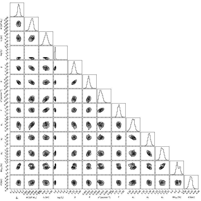
Figure 2: Marginalized and 2D projections of the posterior probability distributions of all model parameters for the fit to NGC 104. Contours indicate $1\sigma$, $2\sigma$ and $3\sigma$ levels on the 2D posterior probability distributions.

Figure 2 shows an example of the resulting posterior distributions for the cluster NGC 104. The best-fitting parameter values for all clusters can be found in Table 2.

The vast majority of marginalized posterior distributions for the cluster parameters follow a unimodal and approximately Gaussian distribution. The marginalized posterior probability distribution of some parameters are skewed towards or hitting the boundaries of the prior ranges, however, as indicated in Section 4.1.2, this is only allowed to occur for parameters with physically motivated prior boundaries.

The posterior parameter distributions of one cluster (NGC 6723) are not single Gaussians, but instead show two separate peaks, both containing comparable posterior probability. This cluster will be discussed in more detail in Paper II, as these models differ most significantly in their BH populations. In all figures in this paper this cluster may appear as a single point with a very large errorbars in one direction, due to the fact that one of these peaks is larger than the other, and the median of the entire distribution falls entirely within this peak.

Two parameters ($\log(\hat{r}_{\mathrm{a}})$ and $\mathrm{BH}_{\mathrm{ret}}$) often have a broader posterior probability distribution. The anisotropy radius may be unconstrained above a certain minimum value, illustrating the fact that all values of the anisotropy radius greater than the truncation radius effectively lead to an entirely isotropic cluster. The BH retention fraction may be completely unconstrained in models with a very small number of BHs initially formed (e.g. due to a "top-light" mass function), in which case the fraction of BHs retained has a negligible effect on the models. These parameters are examined below and in Paper II, respectively.

A fraction of our clusters are core-collapsed, and they are expected to not retain any significant populations of BHs (Giersz & Heggie, 2009; Breen & Heggie, 2013a). However, our best-fitting models of four such clusters (NGC 6266, NGC 6624, NGC 6752, NGC 7078) do possess BHs, and may not be physical. Core-collapsed clusters have a cusp in the inner surface brightness profile which is difficult to reproduce with the limepy models, which are cored. We therefore do not trust the result for BH retention of these clusters as we suspect that $\mathrm{BH}_{\mathrm{ret}}$ was used as an additional degree of freedom in an attempt to describe the inner profiles. In these cases we recompute the models, this time with the amount of retained BHs at the present day fixed to 0 (by fixing the $\mathrm{BH}_{\mathrm{ret}}$ parameter to 0%). These models are used, for these four clusters, in all analysis presented in this paper. This phenomenon, these models and the limitations of our limepy models in representing core-collapsed clusters will all be examined and discussed in more detail in Paper II. However, both sets of models demonstrate good fits to the data, and there was no significant change in the best-fit mass function slopes or in any of the correlations presented in this paper, when considering either set of models.

5.1.2 Best-fitting models

Figures 3 and 4 show an example (also for NGC 104) of the observables predicted by the best-fitting models, overlaid with the observational datasets used to constrain them.

The best-fitting models for the majority of clusters match the given data extraordinarily well. There are, however, a small number of clusters, from our original sample of 37 clusters, where the fits do not reproduce certain datasets adequately. This tends to occur in systems with small amounts of PM and LOS velocity data. Having few kinematic datapoints, as compared to the mass function and number density datasets, means that these models are less able to constrain the non-visible mass and are prone to overfitting the mass functions, at the expense of the kinematics. As fitting both the visible and dark components well is vital to our analysis of the high-mass mass function and the remnant populations, we choose to remove these clusters from our sample going forward. Three such clusters (NGC 4590, NGC 6656, NGC 6981) were discarded due to their unsatisfactory fits. The remaining 34 clusters have best-fitting models that are well matched to all datasets and will make up the set of clusters used in all further analysis.

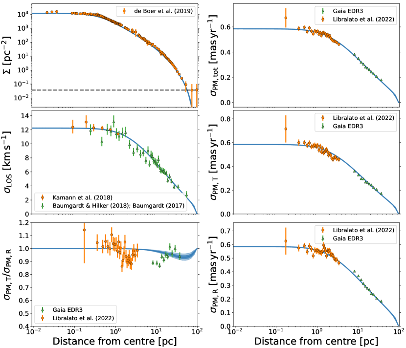
Figure 3: Model radial profiles (blue contours) of surface number density ($\Sigma$), line-of-sight velocity dispersions ($\sigma_{\mathrm{LOS}}$), total ($\sigma_{\mathrm{PM},\mathrm{tot}}$), radial ($\sigma_{\mathrm{PM},\mathrm{R}}$) and tangential ($\sigma_{\mathrm{PM},\mathrm{T}}$) proper motion velocity dispersions and proper motion anisotropy ratio ($\sigma_{\mathrm{PM},\mathrm{T}}/\sigma_{\mathrm{PM},\mathrm{R}}$), for the fit of NGC 104. The dark and light shaded regions represent the $1\sigma$ and $2\sigma$ credible intervals of the model fits, respectively. The observational datasets used to constrain the models are shown alongside their $1\sigma$ uncertainties by the orange and green points and errorbars. The models are fit only on the radial and tangential components of the proper motion individually, while the total and anisotropy ratio are included here solely to demonstrate the fit. The background value subtracted from the number density profile is shown by the dashed line.

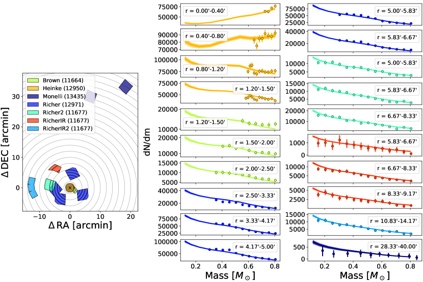
Figure 4: Model local stellar mass functions fit to the observations of NGC 104. Each panel (centre and right columns) shows the number of stars per unit mass as a function of stellar mass, for different distance ranges from the cluster centre. The dark and light shaded regions represent the $1\sigma$ and $2\sigma$ credible intervals of the model fits, respectively. The measurements used to constrain the models are shown alongside their $1\sigma$ uncertainties by the points and errorbars. Each individual HST observing program is denoted by a separate colour, and the corresponding fields for each are shown on the left panel.

Cluster	$\hat{\phi}_{0}$	$M\ [10^{6}\ M_{\odot}]$	$r_{h}\ \left[\mathrm{pc}\right]$	$\log_{10}\left(\hat{r}_{a}\right)$	$g$	$\delta$	$\alpha_{1}$	$\alpha_{2}$	$\alpha_{3}$	$\mathrm{BH}_{\mathrm{ret}}\ \left[\%\right]$	$d\ \left[\mathrm{kpc}\right]$	$s^{2}\ [\mathrm{arcmin^{-4}}]$	$F$
NGC 104	$6.35\begin{subarray}{c}+0.04\\ -0.04\end{subarray}$	$0.894\begin{subarray}{c}+0.003\\ -0.003\end{subarray}$	$6.69\begin{subarray}{c}+0.04\\ -0.04\end{subarray}$	$1.84\begin{subarray}{c}+0.06\\ -0.05\end{subarray}$	$1.53\begin{subarray}{c}+0.02\\ -0.02\end{subarray}$	$0.423\begin{subarray}{c}+0.005\\ -0.005\end{subarray}$	$0.42\begin{subarray}{c}+0.01\\ -0.02\end{subarray}$	$1.37\begin{subarray}{c}+0.02\\ -0.02\end{subarray}$	$2.25\begin{subarray}{c}+0.02\\ -0.01\end{subarray}$	$0.73\begin{subarray}{c}+0.12\\ -0.08\end{subarray}$	$4.416\begin{subarray}{c}+0.009\\ -0.009\end{subarray}$	$0.011\begin{subarray}{c}+0.006\\ -0.005\end{subarray}$	$2.68\begin{subarray}{c}+0.05\\ -0.05\end{subarray}$
NGC 288	$3.68\begin{subarray}{c}+0.09\\ -0.11\end{subarray}$	$0.087\begin{subarray}{c}+0.002\\ -0.002\end{subarray}$	$8.58\begin{subarray}{c}+0.08\\ -0.08\end{subarray}$	$1.0\begin{subarray}{c}+2.0\\ -0.3\end{subarray}$	$0.47\begin{subarray}{c}+0.09\\ -0.06\end{subarray}$	$0.489\begin{subarray}{c}+0.008\\ -0.011\end{subarray}$	$0.42\begin{subarray}{c}+0.03\\ -0.03\end{subarray}$	$1.05\begin{subarray}{c}+0.08\\ -0.07\end{subarray}$	$2.10\begin{subarray}{c}+0.09\\ -0.09\end{subarray}$	$0.2\begin{subarray}{c}+0.4\\ -0.2\end{subarray}$	$8.86\begin{subarray}{c}+0.08\\ -0.08\end{subarray}$	$0.04\begin{subarray}{c}+0.30\\ -0.04\end{subarray}$	$1.44\begin{subarray}{c}+0.07\\ -0.07\end{subarray}$
NGC 362	$5.45\begin{subarray}{c}+0.08\\ -0.04\end{subarray}$	$0.278\begin{subarray}{c}+0.001\\ -0.002\end{subarray}$	$3.44\begin{subarray}{c}+0.03\\ -0.02\end{subarray}$	$1.41\begin{subarray}{c}+0.06\\ -0.05\end{subarray}$	$1.45\begin{subarray}{c}+0.06\\ -0.04\end{subarray}$	$0.484\begin{subarray}{c}+0.005\\ -0.013\end{subarray}$	$0.67\begin{subarray}{c}+0.02\\ -0.01\end{subarray}$	$0.78\begin{subarray}{c}+0.02\\ -0.02\end{subarray}$	$3.01\begin{subarray}{c}+0.03\\ -0.03\end{subarray}$	$5.0\begin{subarray}{c}+0.2\\ -0.3\end{subarray}$	$8.85\begin{subarray}{c}+0.02\\ -0.01\end{subarray}$	$0.00019\begin{subarray}{c}+0.00010\\ -0.00007\end{subarray}$	$2.52\begin{subarray}{c}+0.05\\ -0.04\end{subarray}$
NGC 1261	$3.4\begin{subarray}{c}+0.1\\ -0.1\end{subarray}$	$0.182\begin{subarray}{c}+0.005\\ -0.005\end{subarray}$	$5.00\begin{subarray}{c}+0.07\\ -0.08\end{subarray}$	$1.0\begin{subarray}{c}+1.8\\ -0.2\end{subarray}$	$2.3\begin{subarray}{c}+0.1\\ -0.1\end{subarray}$	$0.48\begin{subarray}{c}+0.01\\ -0.02\end{subarray}$	$1.01\begin{subarray}{c}+0.08\\ -0.08\end{subarray}$	$1.37\begin{subarray}{c}+0.10\\ -0.09\end{subarray}$	$2.7\begin{subarray}{c}+0.2\\ -0.1\end{subarray}$	$2\begin{subarray}{c}+1\\ -1\end{subarray}$	$16.3\begin{subarray}{c}+0.2\\ -0.2\end{subarray}$	$0.000006\begin{subarray}{c}+0.000014\\ -0.000004\end{subarray}$	$4.2\begin{subarray}{c}+0.3\\ -0.3\end{subarray}$
NGC 1851	$5.71\begin{subarray}{c}+0.04\\ -0.03\end{subarray}$	$0.326\begin{subarray}{c}+0.001\\ -0.002\end{subarray}$	$3.68\begin{subarray}{c}+0.02\\ -0.02\end{subarray}$	$4.2\begin{subarray}{c}+0.6\\ -1.0\end{subarray}$	$1.84\begin{subarray}{c}+0.01\\ -0.02\end{subarray}$	$0.491\begin{subarray}{c}+0.007\\ -0.005\end{subarray}$	$0.59\begin{subarray}{c}+0.02\\ -0.02\end{subarray}$	$1.25\begin{subarray}{c}+0.04\\ -0.04\end{subarray}$	$2.88\begin{subarray}{c}+0.05\\ -0.05\end{subarray}$	$2.6\begin{subarray}{c}+0.8\\ -0.4\end{subarray}$	$12.22\begin{subarray}{c}+0.05\\ -0.07\end{subarray}$	$0.000020\begin{subarray}{c}+0.000016\\ -0.000007\end{subarray}$	$2.3\begin{subarray}{c}+0.1\\ -0.1\end{subarray}$
NGC 2808	$4.87\begin{subarray}{c}+0.01\\ -0.01\end{subarray}$	$0.973\begin{subarray}{c}+0.004\\ -0.004\end{subarray}$	$3.959\begin{subarray}{c}+0.006\\ -0.007\end{subarray}$	$1.50\begin{subarray}{c}+0.04\\ -0.05\end{subarray}$	$1.848\begin{subarray}{c}+0.007\\ -0.011\end{subarray}$	$0.495\begin{subarray}{c}+0.002\\ -0.002\end{subarray}$	$0.36\begin{subarray}{c}+0.01\\ -0.01\end{subarray}$	$1.59\begin{subarray}{c}+0.01\\ -0.02\end{subarray}$	$3.12\begin{subarray}{c}+0.04\\ -0.03\end{subarray}$	$11.7\begin{subarray}{c}+0.8\\ -0.4\end{subarray}$	$10.39\begin{subarray}{c}+0.03\\ -0.03\end{subarray}$	$0.000013\begin{subarray}{c}+0.000004\\ -0.000002\end{subarray}$	$2.75\begin{subarray}{c}+0.08\\ -0.11\end{subarray}$
NGC 3201	$4.8\begin{subarray}{c}+0.2\\ -0.2\end{subarray}$	$0.180\begin{subarray}{c}+0.006\\ -0.006\end{subarray}$	$9.9\begin{subarray}{c}+0.5\\ -0.6\end{subarray}$	$0.94\begin{subarray}{c}+0.06\\ -0.05\end{subarray}$	$1.6\begin{subarray}{c}+0.1\\ -0.1\end{subarray}$	$0.45\begin{subarray}{c}+0.03\\ -0.03\end{subarray}$	$1.02\begin{subarray}{c}+0.07\\ -0.08\end{subarray}$	$1.38\begin{subarray}{c}+0.10\\ -0.10\end{subarray}$	$2.15\begin{subarray}{c}+0.08\\ -0.07\end{subarray}$	$0.06\begin{subarray}{c}+0.10\\ -0.04\end{subarray}$	$4.65\begin{subarray}{c}+0.03\\ -0.03\end{subarray}$	$19.0\begin{subarray}{c}+0.7\\ -1.1\end{subarray}$	$2.6\begin{subarray}{c}+0.3\\ -0.2\end{subarray}$
NGC 5024	$5.1\begin{subarray}{c}+0.1\\ -0.1\end{subarray}$	$0.53\begin{subarray}{c}+0.01\\ -0.01\end{subarray}$	$10.5\begin{subarray}{c}+0.2\\ -0.2\end{subarray}$	$7\begin{subarray}{c}+2\\ -2\end{subarray}$	$2.24\begin{subarray}{c}+0.09\\ -0.09\end{subarray}$	$0.32\begin{subarray}{c}+0.03\\ -0.02\end{subarray}$	$0.87\begin{subarray}{c}+0.06\\ -0.06\end{subarray}$	$1.59\begin{subarray}{c}+0.06\\ -0.06\end{subarray}$	$2.4\begin{subarray}{c}+0.1\\ -0.1\end{subarray}$	$2\begin{subarray}{c}+3\\ -1\end{subarray}$	$18.3\begin{subarray}{c}+0.1\\ -0.2\end{subarray}$	$0.002\begin{subarray}{c}+0.003\\ -0.001\end{subarray}$	$2.7\begin{subarray}{c}+0.2\\ -0.1\end{subarray}$
NGC 5139	$2.44\begin{subarray}{c}+0.13\\ -0.07\end{subarray}$	$3.21\begin{subarray}{c}+0.04\\ -0.03\end{subarray}$	$9.62\begin{subarray}{c}+0.06\\ -0.04\end{subarray}$	$6.4\begin{subarray}{c}+0.4\\ -0.7\end{subarray}$	$2.53\begin{subarray}{c}+0.02\\ -0.02\end{subarray}$	$0.426\begin{subarray}{c}+0.006\\ -0.005\end{subarray}$	$0.830\begin{subarray}{c}+0.009\\ -0.008\end{subarray}$	$1.19\begin{subarray}{c}+0.05\\ -0.02\end{subarray}$	$2.16\begin{subarray}{c}+0.04\\ -0.08\end{subarray}$	$20\begin{subarray}{c}+3\\ -5\end{subarray}$	$5.35\begin{subarray}{c}+0.02\\ -0.02\end{subarray}$	$0.00027\begin{subarray}{c}+0.00006\\ -0.00006\end{subarray}$	$6.2\begin{subarray}{c}+0.2\\ -0.1\end{subarray}$
NGC 5272	$5.67\begin{subarray}{c}+0.05\\ -0.02\end{subarray}$	$0.488\begin{subarray}{c}+0.004\\ -0.007\end{subarray}$	$7.04\begin{subarray}{c}+0.06\\ -0.05\end{subarray}$	$5\begin{subarray}{c}+2\\ -1\end{subarray}$	$1.84\begin{subarray}{c}+0.03\\ -0.03\end{subarray}$	$0.306\begin{subarray}{c}+0.002\\ -0.003\end{subarray}$	$1.06\begin{subarray}{c}+0.02\\ -0.02\end{subarray}$	$1.29\begin{subarray}{c}+0.04\\ -0.03\end{subarray}$	$2.24\begin{subarray}{c}+0.06\\ -0.05\end{subarray}$	$1.8\begin{subarray}{c}+0.6\\ -0.4\end{subarray}$	$10.13\begin{subarray}{c}+0.06\\ -0.06\end{subarray}$	$0.000010\begin{subarray}{c}+0.000043\\ -0.000008\end{subarray}$	$2.10\begin{subarray}{c}+0.07\\ -0.08\end{subarray}$
NGC 5904	$5.4\begin{subarray}{c}+0.1\\ -0.1\end{subarray}$	$0.385\begin{subarray}{c}+0.006\\ -0.007\end{subarray}$	$6.35\begin{subarray}{c}+0.08\\ -0.08\end{subarray}$	$5\begin{subarray}{c}+2\\ -2\end{subarray}$	$1.44\begin{subarray}{c}+0.06\\ -0.06\end{subarray}$	$0.45\begin{subarray}{c}+0.03\\ -0.03\end{subarray}$	$0.48\begin{subarray}{c}+0.04\\ -0.04\end{subarray}$	$0.79\begin{subarray}{c}+0.08\\ -0.08\end{subarray}$	$2.27\begin{subarray}{c}+0.06\\ -0.06\end{subarray}$	$0.2\begin{subarray}{c}+0.3\\ -0.2\end{subarray}$	$7.36\begin{subarray}{c}+0.05\\ -0.05\end{subarray}$	$0.006\begin{subarray}{c}+0.010\\ -0.004\end{subarray}$	$4.2\begin{subarray}{c}+0.2\\ -0.2\end{subarray}$
NGC 5986	$4.12\begin{subarray}{c}+0.05\\ -0.06\end{subarray}$	$0.294\begin{subarray}{c}+0.008\\ -0.006\end{subarray}$	$4.41\begin{subarray}{c}+0.04\\ -0.03\end{subarray}$	$1.0\begin{subarray}{c}+2.2\\ -0.1\end{subarray}$	$1.38\begin{subarray}{c}+0.07\\ -0.05\end{subarray}$	$0.492\begin{subarray}{c}+0.005\\ -0.013\end{subarray}$	$0.50\begin{subarray}{c}+0.03\\ -0.03\end{subarray}$	$0.99\begin{subarray}{c}+0.04\\ -0.04\end{subarray}$	$2.41\begin{subarray}{c}+0.07\\ -0.08\end{subarray}$	$0.13\begin{subarray}{c}+0.11\\ -0.08\end{subarray}$	$10.31\begin{subarray}{c}+0.10\\ -0.09\end{subarray}$	$0.00013\begin{subarray}{c}+0.00008\\ -0.00008\end{subarray}$	$2.2\begin{subarray}{c}+0.2\\ -0.1\end{subarray}$
NGC 6093	$6.23\begin{subarray}{c}+0.07\\ -0.08\end{subarray}$	$0.302\begin{subarray}{c}+0.004\\ -0.004\end{subarray}$	$2.38\begin{subarray}{c}+0.02\\ -0.02\end{subarray}$	$6\begin{subarray}{c}+2\\ -2\end{subarray}$	$1.40\begin{subarray}{c}+0.05\\ -0.06\end{subarray}$	$0.34\begin{subarray}{c}+0.02\\ -0.02\end{subarray}$	$0.03\begin{subarray}{c}+0.07\\ -0.07\end{subarray}$	$0.96\begin{subarray}{c}+0.10\\ -0.11\end{subarray}$	$2.48\begin{subarray}{c}+0.05\\ -0.05\end{subarray}$	$4.5\begin{subarray}{c}+0.4\\ -0.6\end{subarray}$	$9.99\begin{subarray}{c}+0.07\\ -0.07\end{subarray}$	$0.009\begin{subarray}{c}+0.003\\ -0.002\end{subarray}$	$3.7\begin{subarray}{c}+0.3\\ -0.3\end{subarray}$
NGC 6121	$6.4\begin{subarray}{c}+0.2\\ -0.1\end{subarray}$	$0.090\begin{subarray}{c}+0.002\\ -0.001\end{subarray}$	$3.90\begin{subarray}{c}+0.06\\ -0.05\end{subarray}$	$7\begin{subarray}{c}+2\\ -3\end{subarray}$	$0.87\begin{subarray}{c}+0.07\\ -0.08\end{subarray}$	$0.46\begin{subarray}{c}+0.02\\ -0.03\end{subarray}$	$-0.10\begin{subarray}{c}+0.08\\ -0.08\end{subarray}$	$0.34\begin{subarray}{c}+0.08\\ -0.08\end{subarray}$	$2.26\begin{subarray}{c}+0.06\\ -0.06\end{subarray}$	$0.4\begin{subarray}{c}+0.2\\ -0.2\end{subarray}$	$1.85\begin{subarray}{c}+0.01\\ -0.01\end{subarray}$	$0.00001\begin{subarray}{c}+0.00006\\ -0.00001\end{subarray}$	$1.28\begin{subarray}{c}+0.08\\ -0.07\end{subarray}$
NGC 6171	$5.57\begin{subarray}{c}+0.08\\ -0.06\end{subarray}$	$0.063\begin{subarray}{c}+0.002\\ -0.002\end{subarray}$	$3.89\begin{subarray}{c}+0.05\\ -0.05\end{subarray}$	$5\begin{subarray}{c}+2\\ -2\end{subarray}$	$0.35\begin{subarray}{c}+0.09\\ -0.09\end{subarray}$	$0.487\begin{subarray}{c}+0.010\\ -0.017\end{subarray}$	$-0.07\begin{subarray}{c}+0.03\\ -0.03\end{subarray}$	$-0.004\begin{subarray}{c}+0.042\\ -0.037\end{subarray}$	$2.34\begin{subarray}{c}+0.07\\ -0.07\end{subarray}$	$0.4\begin{subarray}{c}+0.3\\ -0.2\end{subarray}$	$5.60\begin{subarray}{c}+0.06\\ -0.07\end{subarray}$	$0.004\begin{subarray}{c}+0.002\\ -0.002\end{subarray}$	$1.46\begin{subarray}{c}+0.10\\ -0.09\end{subarray}$
NGC 6205	$3.5\begin{subarray}{c}+0.1\\ -0.1\end{subarray}$	$0.425\begin{subarray}{c}+0.008\\ -0.008\end{subarray}$	$4.51\begin{subarray}{c}+0.04\\ -0.04\end{subarray}$	$6\begin{subarray}{c}+3\\ -3\end{subarray}$	$2.53\begin{subarray}{c}+0.06\\ -0.06\end{subarray}$	$0.41\begin{subarray}{c}+0.04\\ -0.05\end{subarray}$	$0.3\begin{subarray}{c}+0.1\\ -0.1\end{subarray}$	$0.96\begin{subarray}{c}+0.08\\ -0.08\end{subarray}$	$2.38\begin{subarray}{c}+0.08\\ -0.08\end{subarray}$	$4\begin{subarray}{c}+2\\ -1\end{subarray}$	$7.33\begin{subarray}{c}+0.06\\ -0.05\end{subarray}$	$0.00002\begin{subarray}{c}+0.00003\\ -0.00001\end{subarray}$	$2.9\begin{subarray}{c}+0.4\\ -0.3\end{subarray}$
NGC 6218	$5.09\begin{subarray}{c}+0.04\\ -0.05\end{subarray}$	$0.100\begin{subarray}{c}+0.002\\ -0.001\end{subarray}$	$4.13\begin{subarray}{c}+0.04\\ -0.04\end{subarray}$	$4\begin{subarray}{c}+2\\ -2\end{subarray}$	$0.53\begin{subarray}{c}+0.06\\ -0.06\end{subarray}$	$0.496\begin{subarray}{c}+0.003\\ -0.005\end{subarray}$	$0.11\begin{subarray}{c}+0.03\\ -0.04\end{subarray}$	$0.18\begin{subarray}{c}+0.05\\ -0.04\end{subarray}$	$2.81\begin{subarray}{c}+0.05\\ -0.06\end{subarray}$	$3.6\begin{subarray}{c}+0.6\\ -0.7\end{subarray}$	$5.03\begin{subarray}{c}+0.04\\ -0.04\end{subarray}$	$0.00008\begin{subarray}{c}+0.00011\\ -0.00006\end{subarray}$	$2.2\begin{subarray}{c}+0.2\\ -0.2\end{subarray}$
NGC 6254	$5.7\begin{subarray}{c}+0.2\\ -0.2\end{subarray}$	$0.211\begin{subarray}{c}+0.004\\ -0.004\end{subarray}$	$5.18\begin{subarray}{c}+0.07\\ -0.07\end{subarray}$	$3\begin{subarray}{c}+1\\ -1\end{subarray}$	$0.97\begin{subarray}{c}+0.08\\ -0.09\end{subarray}$	$0.41\begin{subarray}{c}+0.04\\ -0.04\end{subarray}$	$0.32\begin{subarray}{c}+0.04\\ -0.05\end{subarray}$	$0.91\begin{subarray}{c}+0.08\\ -0.08\end{subarray}$	$2.20\begin{subarray}{c}+0.07\\ -0.06\end{subarray}$	$0.3\begin{subarray}{c}+0.4\\ -0.2\end{subarray}$	$5.10\begin{subarray}{c}+0.04\\ -0.04\end{subarray}$	$0.0003\begin{subarray}{c}+0.0002\\ -0.0002\end{subarray}$	$2.7\begin{subarray}{c}+0.2\\ -0.2\end{subarray}$
NGC 6266	$5.6\begin{subarray}{c}+0.1\\ -0.2\end{subarray}$	$0.75\begin{subarray}{c}+0.02\\ -0.01\end{subarray}$	$3.17\begin{subarray}{c}+0.07\\ -0.06\end{subarray}$	$1.38\begin{subarray}{c}+0.12\\ -0.07\end{subarray}$	$0.91\begin{subarray}{c}+0.06\\ -0.05\end{subarray}$	$0.498\begin{subarray}{c}+0.002\\ -0.003\end{subarray}$	$0.2\begin{subarray}{c}+0.2\\ -0.2\end{subarray}$	$1.24\begin{subarray}{c}+0.07\\ -0.06\end{subarray}$	$2.24\begin{subarray}{c}+0.03\\ -0.04\end{subarray}$	—	$6.50\begin{subarray}{c}+0.04\\ -0.03\end{subarray}$	$0.22\begin{subarray}{c}+0.02\\ -0.02\end{subarray}$	$2.5\begin{subarray}{c}+0.3\\ -0.3\end{subarray}$
NGC 6341	$5.4\begin{subarray}{c}+0.4\\ -0.3\end{subarray}$	$0.300\begin{subarray}{c}+0.007\\ -0.005\end{subarray}$	$4.20\begin{subarray}{c}+0.06\\ -0.07\end{subarray}$	$6\begin{subarray}{c}+3\\ -3\end{subarray}$	$1.78\begin{subarray}{c}+0.05\\ -0.06\end{subarray}$	$0.43\begin{subarray}{c}+0.04\\ -0.05\end{subarray}$	$0.81\begin{subarray}{c}+0.04\\ -0.04\end{subarray}$	$1.09\begin{subarray}{c}+0.09\\ -0.09\end{subarray}$	$2.21\begin{subarray}{c}+0.08\\ -0.08\end{subarray}$	$0.7\begin{subarray}{c}+0.3\\ -0.4\end{subarray}$	$8.42\begin{subarray}{c}+0.06\\ -0.06\end{subarray}$	$0.00007\begin{subarray}{c}+0.00007\\ -0.00004\end{subarray}$	$3.7\begin{subarray}{c}+0.2\\ -0.2\end{subarray}$
NGC 6352	$6.6\begin{subarray}{c}+0.2\\ -0.1\end{subarray}$	$0.098\begin{subarray}{c}+0.006\\ -0.006\end{subarray}$	$8.7\begin{subarray}{c}+0.7\\ -0.7\end{subarray}$	$7\begin{subarray}{c}+2\\ -2\end{subarray}$	$0.2\begin{subarray}{c}+0.2\\ -0.1\end{subarray}$	$0.491\begin{subarray}{c}+0.007\\ -0.013\end{subarray}$	$0.25\begin{subarray}{c}+0.10\\ -0.10\end{subarray}$	$0.66\begin{subarray}{c}+0.09\\ -0.10\end{subarray}$	$1.99\begin{subarray}{c}+0.05\\ -0.06\end{subarray}$	$0.16\begin{subarray}{c}+0.04\\ -0.04\end{subarray}$	$5.62\begin{subarray}{c}+0.06\\ -0.06\end{subarray}$	$2.04\begin{subarray}{c}+0.05\\ -0.03\end{subarray}$	$2.1\begin{subarray}{c}+0.2\\ -0.1\end{subarray}$
NGC 6362	$4.14\begin{subarray}{c}+0.13\\ -0.10\end{subarray}$	$0.111\begin{subarray}{c}+0.003\\ -0.003\end{subarray}$	$6.95\begin{subarray}{c}+0.09\\ -0.09\end{subarray}$	$4\begin{subarray}{c}+2\\ -2\end{subarray}$	$0.5\begin{subarray}{c}+0.2\\ -0.2\end{subarray}$	$0.46\begin{subarray}{c}+0.02\\ -0.04\end{subarray}$	$0.26\begin{subarray}{c}+0.04\\ -0.04\end{subarray}$	$0.64\begin{subarray}{c}+0.07\\ -0.07\end{subarray}$	$1.84\begin{subarray}{c}+0.07\\ -0.07\end{subarray}$	$0.03\begin{subarray}{c}+0.05\\ -0.03\end{subarray}$	$7.63\begin{subarray}{c}+0.06\\ -0.06\end{subarray}$	$16\begin{subarray}{c}+3\\ -4\end{subarray}$	$1.57\begin{subarray}{c}+0.11\\ -0.09\end{subarray}$
NGC 6366	$4.0\begin{subarray}{c}+0.1\\ -0.1\end{subarray}$	$0.032\begin{subarray}{c}+0.001\\ -0.001\end{subarray}$	$4.62\begin{subarray}{c}+0.09\\ -0.09\end{subarray}$	$2\begin{subarray}{c}+2\\ -1\end{subarray}$	$0.6\begin{subarray}{c}+0.2\\ -0.2\end{subarray}$	$0.488\begin{subarray}{c}+0.009\\ -0.017\end{subarray}$	$-0.30\begin{subarray}{c}+0.07\\ -0.08\end{subarray}$	$-0.19\begin{subarray}{c}+0.08\\ -0.07\end{subarray}$	$3.1\begin{subarray}{c}+0.2\\ -0.2\end{subarray}$	$4\begin{subarray}{c}+5\\ -3\end{subarray}$	$3.38\begin{subarray}{c}+0.04\\ -0.04\end{subarray}$	$0.002\begin{subarray}{c}+0.002\\ -0.001\end{subarray}$	$1.25\begin{subarray}{c}+0.09\\ -0.08\end{subarray}$
NGC 6397	$7.86\begin{subarray}{c}+0.09\\ -0.09\end{subarray}$	$0.108\begin{subarray}{c}+0.002\\ -0.002\end{subarray}$	$4.9\begin{subarray}{c}+0.1\\ -0.1\end{subarray}$	$2.7\begin{subarray}{c}+0.1\\ -0.1\end{subarray}$	$1.58\begin{subarray}{c}+0.07\\ -0.07\end{subarray}$	$0.497\begin{subarray}{c}+0.002\\ -0.003\end{subarray}$	$0.60\begin{subarray}{c}+0.04\\ -0.04\end{subarray}$	$0.69\begin{subarray}{c}+0.07\\ -0.05\end{subarray}$	$2.42\begin{subarray}{c}+0.04\\ -0.03\end{subarray}$	$0.14\begin{subarray}{c}+0.01\\ -0.01\end{subarray}$	$2.43\begin{subarray}{c}+0.01\\ -0.01\end{subarray}$	$8.8\begin{subarray}{c}+0.8\\ -1.2\end{subarray}$	$2.1\begin{subarray}{c}+0.1\\ -0.1\end{subarray}$
NGC 6541	$6.03\begin{subarray}{c}+0.06\\ -0.04\end{subarray}$	$0.220\begin{subarray}{c}+0.002\\ -0.002\end{subarray}$	$3.49\begin{subarray}{c}+0.03\\ -0.02\end{subarray}$	$3.85\begin{subarray}{c}+0.09\\ -0.07\end{subarray}$	$1.33\begin{subarray}{c}+0.01\\ -0.02\end{subarray}$	$0.470\begin{subarray}{c}+0.002\\ -0.003\end{subarray}$	$0.30\begin{subarray}{c}+0.01\\ -0.01\end{subarray}$	$1.18\begin{subarray}{c}+0.05\\ -0.05\end{subarray}$	$2.107\begin{subarray}{c}+0.009\\ -0.009\end{subarray}$	$0.006\begin{subarray}{c}+0.007\\ -0.005\end{subarray}$	$7.491\begin{subarray}{c}+0.009\\ -0.011\end{subarray}$	$0.0003\begin{subarray}{c}+0.0002\\ -0.0001\end{subarray}$	$4.45\begin{subarray}{c}+0.08\\ -0.08\end{subarray}$
NGC 6624	$11.0\begin{subarray}{c}+0.2\\ -0.2\end{subarray}$	$0.102\begin{subarray}{c}+0.003\\ -0.003\end{subarray}$	$2.13\begin{subarray}{c}+0.05\\ -0.04\end{subarray}$	$2.91\begin{subarray}{c}+0.07\\ -0.07\end{subarray}$	$1.2\begin{subarray}{c}+0.1\\ -0.1\end{subarray}$	$0.496\begin{subarray}{c}+0.003\\ -0.004\end{subarray}$	$-0.70\begin{subarray}{c}+0.09\\ -0.09\end{subarray}$	$-0.50\begin{subarray}{c}+0.05\\ -0.05\end{subarray}$	$2.40\begin{subarray}{c}+0.05\\ -0.06\end{subarray}$	—	$8.11\begin{subarray}{c}+0.08\\ -0.06\end{subarray}$	$0.3\begin{subarray}{c}+0.1\\ -0.1\end{subarray}$	$1.2\begin{subarray}{c}+0.1\\ -0.1\end{subarray}$
NGC 6681	$7.28\begin{subarray}{c}+0.08\\ -0.06\end{subarray}$	$0.096\begin{subarray}{c}+0.002\\ -0.002\end{subarray}$	$2.67\begin{subarray}{c}+0.05\\ -0.05\end{subarray}$	$1.82\begin{subarray}{c}+0.10\\ -0.07\end{subarray}$	$1.16\begin{subarray}{c}+0.06\\ -0.08\end{subarray}$	$0.487\begin{subarray}{c}+0.009\\ -0.009\end{subarray}$	$-0.13\begin{subarray}{c}+0.08\\ -0.09\end{subarray}$	$0.13\begin{subarray}{c}+0.08\\ -0.10\end{subarray}$	$2.04\begin{subarray}{c}+0.05\\ -0.04\end{subarray}$	$0.10\begin{subarray}{c}+0.02\\ -0.01\end{subarray}$	$9.46\begin{subarray}{c}+0.04\\ -0.05\end{subarray}$	$0.05\begin{subarray}{c}+0.01\\ -0.01\end{subarray}$	$3.2\begin{subarray}{c}+0.2\\ -0.2\end{subarray}$
NGC 6723	$3.74\begin{subarray}{c}+0.92\\ -0.08\end{subarray}$	$0.177\begin{subarray}{c}+0.017\\ -0.002\end{subarray}$	$5.12\begin{subarray}{c}+0.05\\ -0.03\end{subarray}$	$0.35\begin{subarray}{c}+2.57\\ -0.02\end{subarray}$	$0.59\begin{subarray}{c}+0.65\\ -0.07\end{subarray}$	$0.31\begin{subarray}{c}+0.09\\ -0.01\end{subarray}$	$0.10\begin{subarray}{c}+0.02\\ -0.02\end{subarray}$	$0.34\begin{subarray}{c}+0.06\\ -0.03\end{subarray}$	$2.360\begin{subarray}{c}+0.009\\ -0.328\end{subarray}$	$4.6\begin{subarray}{c}+0.5\\ -4.5\end{subarray}$	$8.388\begin{subarray}{c}+0.068\\ -0.008\end{subarray}$	$13.6\begin{subarray}{c}+0.6\\ -0.3\end{subarray}$	$2.36\begin{subarray}{c}+0.06\\ -0.80\end{subarray}$
NGC 6752	$6.07\begin{subarray}{c}+0.06\\ -0.05\end{subarray}$	$0.211\begin{subarray}{c}+0.004\\ -0.003\end{subarray}$	$3.54\begin{subarray}{c}+0.04\\ -0.04\end{subarray}$	$1.54\begin{subarray}{c}+0.02\\ -0.02\end{subarray}$	$1.64\begin{subarray}{c}+0.02\\ -0.02\end{subarray}$	$0.496\begin{subarray}{c}+0.003\\ -0.004\end{subarray}$	$0.45\begin{subarray}{c}+0.05\\ -0.06\end{subarray}$	$0.51\begin{subarray}{c}+0.04\\ -0.04\end{subarray}$	$2.08\begin{subarray}{c}+0.04\\ -0.04\end{subarray}$	—	$4.04\begin{subarray}{c}+0.03\\ -0.02\end{subarray}$	$0.00003\begin{subarray}{c}+0.00003\\ -0.00002\end{subarray}$	$5.1\begin{subarray}{c}+0.2\\ -0.2\end{subarray}$
NGC 6779	$5.88\begin{subarray}{c}+0.05\\ -0.05\end{subarray}$	$0.168\begin{subarray}{c}+0.004\\ -0.004\end{subarray}$	$5.38\begin{subarray}{c}+0.07\\ -0.07\end{subarray}$	$2.8\begin{subarray}{c}+0.8\\ -0.6\end{subarray}$	$1.00\begin{subarray}{c}+0.10\\ -0.10\end{subarray}$	$0.314\begin{subarray}{c}+0.010\\ -0.008\end{subarray}$	$0.57\begin{subarray}{c}+0.05\\ -0.05\end{subarray}$	$0.86\begin{subarray}{c}+0.07\\ -0.07\end{subarray}$	$2.30\begin{subarray}{c}+0.06\\ -0.06\end{subarray}$	$3.4\begin{subarray}{c}+0.6\\ -0.6\end{subarray}$	$10.13\begin{subarray}{c}+0.04\\ -0.05\end{subarray}$	$0.0003\begin{subarray}{c}+0.0002\\ -0.0002\end{subarray}$	$2.9\begin{subarray}{c}+0.1\\ -0.1\end{subarray}$
NGC 6809	$3.09\begin{subarray}{c}+0.07\\ -0.06\end{subarray}$	$0.183\begin{subarray}{c}+0.005\\ -0.004\end{subarray}$	$6.18\begin{subarray}{c}+0.05\\ -0.05\end{subarray}$	$6\begin{subarray}{c}+3\\ -3\end{subarray}$	$1.26\begin{subarray}{c}+0.07\\ -0.08\end{subarray}$	$0.488\begin{subarray}{c}+0.009\\ -0.015\end{subarray}$	$0.50\begin{subarray}{c}+0.03\\ -0.03\end{subarray}$	$0.58\begin{subarray}{c}+0.05\\ -0.05\end{subarray}$	$2.6\begin{subarray}{c}+0.1\\ -0.1\end{subarray}$	$0.7\begin{subarray}{c}+0.5\\ -0.4\end{subarray}$	$5.25\begin{subarray}{c}+0.03\\ -0.04\end{subarray}$	$0.0005\begin{subarray}{c}+0.0005\\ -0.0003\end{subarray}$	$2.8\begin{subarray}{c}+0.2\\ -0.2\end{subarray}$
NGC 7078	$8.8\begin{subarray}{c}+0.2\\ -0.2\end{subarray}$	$0.614\begin{subarray}{c}+0.007\\ -0.007\end{subarray}$	$5.17\begin{subarray}{c}+0.05\\ -0.04\end{subarray}$	$3.02\begin{subarray}{c}+0.08\\ -0.09\end{subarray}$	$1.61\begin{subarray}{c}+0.07\\ -0.09\end{subarray}$	$0.46\begin{subarray}{c}+0.01\\ -0.01\end{subarray}$	$0.80\begin{subarray}{c}+0.04\\ -0.04\end{subarray}$	$1.75\begin{subarray}{c}+0.06\\ -0.06\end{subarray}$	$1.94\begin{subarray}{c}+0.04\\ -0.04\end{subarray}$	—	$10.69\begin{subarray}{c}+0.06\\ -0.06\end{subarray}$	$0.00004\begin{subarray}{c}+0.00003\\ -0.00002\end{subarray}$	$3.1\begin{subarray}{c}+0.2\\ -0.2\end{subarray}$
NGC 7089	$4.9\begin{subarray}{c}+0.2\\ -0.2\end{subarray}$	$0.627\begin{subarray}{c}+0.009\\ -0.009\end{subarray}$	$4.59\begin{subarray}{c}+0.07\\ -0.07\end{subarray}$	$9\begin{subarray}{c}+4\\ -4\end{subarray}$	$1.92\begin{subarray}{c}+0.06\\ -0.07\end{subarray}$	$0.43\begin{subarray}{c}+0.04\\ -0.04\end{subarray}$	$0.5\begin{subarray}{c}+0.1\\ -0.1\end{subarray}$	$1.14\begin{subarray}{c}+0.07\\ -0.07\end{subarray}$	$2.97\begin{subarray}{c}+0.08\\ -0.08\end{subarray}$	$12\begin{subarray}{c}+4\\ -4\end{subarray}$	$11.53\begin{subarray}{c}+0.08\\ -0.07\end{subarray}$	$0.00006\begin{subarray}{c}+0.00005\\ -0.00003\end{subarray}$	$3.0\begin{subarray}{c}+0.3\\ -0.3\end{subarray}$
NGC 7099	$6.3645\begin{subarray}{c}+0.0004\\ -0.0003\end{subarray}$	$0.14210\begin{subarray}{c}+0.00003\\ -0.00004\end{subarray}$	$4.529\begin{subarray}{c}+0.005\\ -0.011\end{subarray}$	$1.6758\begin{subarray}{c}+0.0009\\ -0.0019\end{subarray}$	$1.172\begin{subarray}{c}+0.003\\ -0.008\end{subarray}$	$0.4931\begin{subarray}{c}+0.0001\\ -0.0003\end{subarray}$	$0.499\begin{subarray}{c}+0.002\\ -0.001\end{subarray}$	$1.169\begin{subarray}{c}+0.003\\ -0.006\end{subarray}$	$2.2312\begin{subarray}{c}+0.0004\\ -0.0009\end{subarray}$	$0.1152\begin{subarray}{c}+0.0001\\ -0.0001\end{subarray}$	$8.445\begin{subarray}{c}+0.002\\ -0.001\end{subarray}$	$0.00005\begin{subarray}{c}+0.00002\\ -0.00003\end{subarray}$	$3.65\begin{subarray}{c}+0.03\\ -0.01\end{subarray}$

Table 2: Median and $1\sigma$ uncertainties of all best-fitting model, mass function and nuisance parameters, for all clusters. Empty dashes in the $\mathrm{BH}_{\mathrm{ret}}$ column represent the four core-collapsed clusters with a value fixed to 0. Note that all uncertainties presented here represent only the statistical uncertainties on the fits, and likely underestimate the true uncertainties. See sections 5.2 and 6.1.1 for more details.

5.2 Cluster Parameters

Given this set of best-fitting models, we next examine the distributions of various model parameters and compare with other results from the literature. The best-fitting model, mass function and nuisance parameters for all clusters are shown in Table 2.

It must be noted here that all uncertainties presented for these parameters, in this entire analysis, are accounting solely for the statistical uncertainties on the parameter fits. Our fitting procedure operates under the assumption that our models are a good representation of the data, and as such may, in reality, be underestimating the true errors. It has been shown that multimass DF models, such as those used here, may underestimate the uncertainties when compared to more flexible models, such as Jeans models (Hénault-Brunet et al., 2019), which could be indicative of systematic errors not captured in the statistical uncertainties and limitations in the ability of these models to perfectly reproduce the data.

5.2.1 Comparison with literature

To begin, we can compare our best-fitting models with other comprehensive studies of Milky Way GCs in the literature. Namely, we consider in Figure 5 the distances determined by Vasiliev & Baumgardt (2021), and the total masses and half-mass radii inferred from the $N$-body model fits of Baumgardt et al. (2023). The top panels of Figure 5 shows the relation between the literature values and our own, demonstrating a good general agreement and no obvious biases, but with noticeable spread around the lines of perfect agreement. This is reinforced in the bottom panels, which show the distribution of the fractional differences between our values, divided by their combined uncertainties. If the agreement was perfect, and all systematic errors were accounted for in our uncertainties, this distribution would resemble a Gaussian centred at 0 with a width of $\sigma=1$ (shown by the dashed black line). Our distributions, meanwhile, are roughly centred near 0 but, in the case of mass and half-mass radius, show a much wider spread. This increased width demonstrates that the combined systematic uncertainties of both our values and the literature values are underestimated by a factor of a few.

It should be noted that the excellent agreement with the heliocentric distances of Vasiliev & Baumgardt (2021) is largely by design, given our use of a Gaussian centred on their values as the prior on the distance parameter (see Section 4.1.2), but this does still indicate that our models and observations are perfectly compatible with those distances.

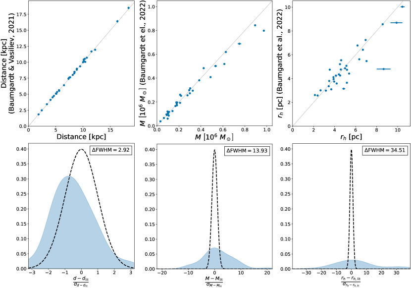
Figure 5: Comparison of the heliocentric distance, total system mass, and half-mass radius of all cluster fits against the distances computed by Vasiliev & Baumgardt (2021) and the properties inferred from the $N$-body model fits of Baumgardt et al. (2023). The top row compares the median and $1\sigma$ values of both both sources, with the grey diagonal representing perfect agreement. The bottom row shows the distribution (represented by a Gaussian KDE) of the fractional differences among all clusters, divided by their combined uncertainties. The dashed black line shows a Gaussian, centred on 0 with a width of $\sigma=1$, which represents perfect agreement. The ratio of the FWHM of the fractional difference distributions to that of the Gaussian is noted in the top right corners. NGC 5139 is excluded from these figures due to its very large mass but shows similar agreement, and will be discussed in more detail in Paper II.

5.2.2 Anisotropy

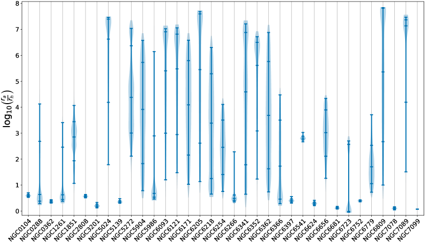
Figure 6: Violin plot of the posterior distribution of the (log) anisotropy radius, normalized by the cluster half-mass radius, for all clusters. The median, $1\sigma$ and $2\sigma$ values are denoted by the horizontal ticks on each distribution.

Figure 6 shows the distribution of the anisotropy radius (normalized by the half-mass radius) for all clusters. It is immediately clear from this plot that there are two populations of anisotropy results in our fits; distributions with a clear peak, constrained to a narrow range of best-fitting values, and very broad, flat distributions with no clear peak above a certain minimum value, extending up to the prior bounds. As described in Section 2.1, clusters where $r_{\mathrm{a}}$ is more clearly peaked favour a certain amount of radial anisotropy, whereas clusters with broad posterior distributions are effectively isotropic, as all values of $r_{\mathrm{a}}$ above the minima of the broad distributions (corresponding to approximately at or above the truncation radius) essentially lead to the same isotropic model. Values above this minimum therefore have a negligible effect on the computed model likelihoods.

It should be noted that the constraints we can place on velocity anisotropy come entirely from the Gaia and HST proper motion dispersion profiles. These datasets are quite limited in many clusters, and as such some of the clusters with broad distributions may not actually be entirely isotropic in reality, but simply cannot be sufficiently constrained by the data currently available. It is also important to note that our limepy models are unable to reproduce any amount of tangential anisotropy (Gieles & Zocchi, 2015), and instead, when tangentially biased anisotropy is present in our data. the models will favour a mostly isotropic fit as a compromise between the radial and tangential regimes (Peuten et al., 2017).

It is clear, based on the wide range of $\log(r_{\mathrm{a}})$ values, that allowing the anisotropy radius to vary freely is necessary to best model the GCs. The degree of anisotropy in a cluster is important for understanding the central dark remnant populations, as there exists a degeneracy between the observational fingerprints of central dark mass and velocity anisotropy, when observational constraints on only one component of velocity are available (Evans et al., 2009; Zocchi et al., 2017).

6 Mass Functions

In this section, we explore the mass function exponents inferred from our model fits. We will examine the relationships between the MF exponents, discuss the connection between the global mass function probed by our models and the initial stellar mass function of GCs, and search for any possible correlations between the IMF and environment of globular clusters.

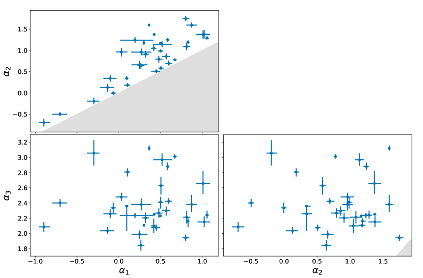
Figure 7: Relations between all three mass function exponent parameters. Gray shaded areas represent the parameter space which is disallowed by the priors on the mass function slopes.

To begin, we examine the distribution of the $\alpha$ parameters between all clusters. Figure 7 shows the relationships between all three mass function slopes ($\alpha_{1},\alpha_{2},\alpha_{3}$). The high-mass $\alpha_{3}$ is not clearly correlated to either of the other MF exponents, however a clear relation can be seen between $\alpha_{1}$ and $\alpha_{2}$. While it should be noted that, by design, the priors used here disallow $\alpha_{1}<\alpha_{2}$ (as shown by the shaded regions in Figure 7), which may introduce a bias to this trend (although, as mentioned before, tests of clusters near this bound fit without this constraint resulted in negligible changes), it is clear that, in general, clusters with a more depleted low-mass mass function also have a relatedly depleted intermediate-mass mass function.

The relation between $\alpha_{1}$ and $\alpha_{2}$ also showcases another important phenomenon; a large number of clusters do not fall on or near the $\alpha_{1}=\alpha_{2}$ line, but are instead steeper in the intermediate-mass regime than the low-mass regime. This suggests that a two-component power law is necessary to describe the global mass function below $1\text{\,}\mathrm{M}_{\odot}$, and a single power law attempting to describe the same mass regime would overestimate both the high and low mass ends of the mass function in this regime, and underestimate the mass function in the intermediate regime, near the break mass of $0.5\text{\,}\mathrm{M}_{\odot}$. That is, a single $\alpha$ power law over the same mass domain would have a slope greater than $\alpha_{1}$ and less than $\alpha_{2}$.

6.1 Initial mass function

The $\alpha$ parameters constrained by the models describe the global stellar mass functions of the clusters at the present day, and in order to examine the initial mass function of our clusters we must carefully consider the connection between the IMF and the PDMF. As discussed in Section 2.2, we have chosen not to model the dynamical loss of (preferentially low-mass) stars in the mass function evolution algorithm used, due to its complex dependence on the dynamical evolution and initial conditions of the cluster. Therefore, in our models, the IMF can most directly be inferred only in the high-mass ($\alpha_{3},m>$1\text{\,}\mathrm{M}_{\odot}$$) regime, while the lower-mass exponents ($\alpha_{1},\alpha_{2}$) are more representative of the present-day mass function, which may have evolved away from the IMF significantly.

To quantify this assertion, we must examine the dynamical evolution of our clusters, as the dynamical loss of stars is not necessarily limited entirely to the lower-mass regime. In very dynamically evolved clusters, which have lost a substantial amount of their total initial mass to escaping stars, the characteristic mass of preferentially escaping stars will increase, potentially depleting even the population of higher-mass stars and WDs, which had initial masses above , and in such cases the inferred mass function exponent $\alpha_{3}$ may also be shallower and less directly representative of the IMF. To account for this effect, we must determine which clusters have lost a large amount of their initial mass by the present day. We estimate this remaining mass fraction by the equation:

$$\frac{M_{\mathrm{today}}}{M_{\mathrm{initial}}}=0.55\times\left(1-\frac{\mathrm{Age}}{\tau_{\mathrm{diss}}}\right)$$ (25)

where the factor 0.55 reflects the typically assumed mass loss from stellar evolution of $\sim 55\%$ of the initial cluster mass in the first Gyr of a cluster’s evolution and the dissolution time $\tau_{\mathrm{diss}}$ represents the estimated total lifetime of the cluster. The estimated lifetimes of our clusters were computed according to the approach described in Section 3.2 of Baumgardt et al. (2019), using the updated models of Baumgardt et al. (2023). This method is based on integrating the orbit of the clusters backwards in the Milky Way galactic potential (Irrgang et al., 2013), and estimating the resulting mass loss. A related quantity is the “dynamical age”, which we define as the ratio of the cluster’s age over its half-mass relaxation time ($\tau_{\mathrm{rel}}$).

We have taken both the relaxation and dissolution times from the best-fitting models of Baumgardt et al. (2023), a companion study which determined the mass functions of 120 MW, LMC and SMC globular clusters by comparing the same HST mass function datasets as used in this work with a grid of direct $N$-body simulations. While we could technically extract the relaxation times self-consistently from our own set of models, we utilize the values obtained by Baumgardt et al. (2023) in order to most easily compare our results. Given the good agreement (on average) between total mass and half-mass radii of their $N$-body models, as shown in Figure 5, the differences should be negligible.

These quantities, and their relationships with all mass function exponents, are shown for all clusters in Figure 8. The clusters to the left of these plots are thought to have lost a large amount of their initial mass and be more dynamically evolved. In these cases the lower-mass $\alpha_{1}$ and $\alpha_{2}$ slopes are shallower (even becoming negative in the most dynamically evolved clusters), and the $\alpha_{3}$ slope may also have been modified by dynamical evolution. As such, caution is advised when interpreting the slopes in these clusters as representative of the IMF. These quantities cannot be used to define an exact division of where the global mass function parameters reflect the IMF, but it does provide useful context to our proceeding analysis of the IMF.

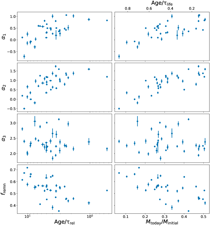
Figure 8: Relations between all three mass function exponent parameters and the fraction of cluster mass in all stellar remnants (white dwarfs, neutron stars, black holes) versus the dynamical age and remaining mass fraction of all clusters. Clusters with higher remaining mass fractions and relaxation times greater than their ages provide more reliable probes of the IMF.

We can clearly see that both lower-mass MF exponents ($\alpha_{1}$, $\alpha_{2}$) have distinct correlations with these two quantities, with the increasingly evolved clusters (short lifetimes / relaxation times compared to their ages) substantially more depleted in low-mass stars than their less evolved counterparts. This trend, and the IMF in the low and intermediate-mass regime are explored in more detail in Baumgardt et al. (2023). No such correlation exists with $\alpha_{3}$, which supports our assertion that the high-mass regime is less affected by the cluster’s dynamical evolution, and thus, overall, most representative of the IMF. However, as stated before, caution should still be applied when interpreting the $\alpha_{3}$ of the clusters to the left side of this figure. We will examine this parameter in more detail in Section 6.1.1 below.

The evolution of the remnant mass fraction $f_{\mathrm{remn}}$, which includes all types of stellar remnants, is also shown at the bottom of Figure 8, where a strong relationship with the dynamical age of the clusters is evident, as might be expected. As a cluster evolves and loses mass, as mentioned before, the mass lost is preferentially in the form of lower-mass stars, rather than the heavy remnants, and as such the fraction of mass in remnants should increase as the cluster’s low-mass MF is depleted. Interestingly, some of the most dynamically evolved clusters have nearly 75% of their mass in dark remnants at the present day, which could have important implications for the mass-to-light ratios and inferred masses of unresolved GCs in distant galaxies.

6.1.1 High-mass IMF

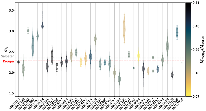
Figure 9: Violin plot of the $\alpha_{3}$ parameter posterior distributions for all clusters. The median, $1\sigma$ and $2\sigma$ values are denoted by the horizontal ticks on each distribution. Colours represent the remaining mass fraction. The corresponding values of some canonical high-mass ($m>$1\text{\,}\mathrm{M}_{\odot}$$) IMF formulations (Salpeter, 1955; Kroupa, 2001) are shown by dashed lines.

Figure 9 shows the posterior probability distributions of $\alpha_{3}$ for all clusters. From this figure we can see that the distributions are, in the vast majority of cases, compatible within uncertainties with the typically assumed canonical high-mass ($m>$1\text{\,}\mathrm{M}_{\odot}$$) IMF formulations (e.g. Salpeter, 1955; Kroupa, 2001), however with a large spread of $\alpha_{3}$ values between $\sim 2\mathrm{-}3$. The median and $1\sigma$ values over all clusters are $\alpha_{3}=2.37\begin{subarray}{c}+0.48\\ -0.25\end{subarray}$. This matches remarkably well with the canonical IMFs, a striking result given the large freedom in the mass function of our models. This result is also in agreement with the high-mass slopes determined by Baumgardt et al. (2023) through the examination of similar HST mass function datasets in younger clusters in the Large (LMC) and Small Magellanic Clouds (SMC), where more massive stars, yet to evolve off the main sequence, can still be observed directly. Similar results were also obtained by Weisz et al. (2015) for young clusters in M 31. It is even clearer that our fits do not favour any more extreme IMFs, neither exceedingly top-heavy nor top-light, especially when ignoring the most dynamically evolved clusters (shown in Figure 9 by the more yellow colours).

This result is counter to some recent suggestions in the literature of top-heavy IMFs in GCs. It has been shown that clusters with top-heavy IMFs are expected to have lost a very large fraction of their mass early in their lifetimes due to stellar mass loss and supernova explosions (Haghi et al., 2020), produce a large amount of BHs and could contribute significantly to the observed rate of binary BH mergers (Weatherford et al., 2021; Antonini et al., 2022). Given that our results seem to preclude any clusters as top-heavy as $\alpha_{3}\sim 1.6$, there is thus no obvious need to consider top-heavy IMFs in estimates of BBH merger rates in globular clusters. Due to the smaller dissolution times of top-heavy GCs of typical masses ($\sim 10^{5}\ \mathrm{M}_{\odot}$), there remains the possibility that some GCs had formed with a more top-heavy IMF, and have simply dissolved to such an extent by the present day that they are undetectable. These clusters could still contribute significantly to the rate of BBH mergers and gravitational waves. However, given the large range of GC parameter space covered by our models, it is unclear what would cause these top-heavy GCs to form alongside clusters with a more canonical IMF as we see here. As shown in Haghi et al. (2020), the dissolution times of GCs scale smoothly with the IMF, resulting in, for example, lifetimes $\sim 3$ times shorter for typical-mass clusters with $\alpha_{3}\approx 1.8$, compared to clusters with a canonical IMF. Given that the spread in initial masses of the GC population is likely on the order of $\sim 100$ (e.g. Balbinot & Gieles, 2018), we would expect to still find some surviving clusters with an $\alpha_{3}<1.8$, if they had formed alongside our sample.

It should be noted again that, as mentioned in Section 5.2, the uncertainties on these parameters represent only the statistical uncertainties on the fits, and the actual errors could be larger. This extra uncertainty on the model would be difficult to quantify exactly, however, examining in particular $\alpha_{3}$, based on a reduced chi-squared test, if all the scatter in these results (away from the mean) were explained by the uncertainties in our models (beyond the statistical uncertainties shown), it would indicate a typical error of approximately 0.4 on $\alpha_{3}$.

6.2 Relationship with metallicity

We next examine possible correlations between the high-mass stellar IMF of GCs and metallicity. Variations of the initial mass function with metallicity have been suggested in the past based on theoretical studies of star and cluster formation, which indicate that increasing metallicity leads to more efficient cooling and helps limit stellar accretion, and thus should reduce the characteristic mass of formed stars and produce an increasingly bottom-heavy IMF in more metal-rich clusters (Larson, 1998; De Marchi et al., 2017; Chon et al., 2021). Marks et al. (2012) proposed a linear relationship between the high-mass IMF slope and metallicity, which begins with more top-heavy values of $\alpha_{3}$ at lower metallicities ($\alpha_{3}=1$ at $[\mathrm{Fe}/\mathrm{H}]=-2.5$), and reaches the canonical Kroupa value of 2.3 only at metallicities $[\mathrm{Fe}/\mathrm{H}]>-0.5$. Given the large amount of freedom available in our mass function slopes, and the excellent constraints we are able to place on the dark remnant populations in this mass regime, our model fits, which span nearly the full range of Milky Way GC metallicities, present an excellent opportunity to examine this potential relationship.

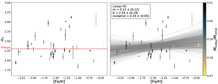
Figure 10: Relation between the high-mass IMF exponent $\alpha_{3}$ and the cluster metallicity for all clusters. Colours represent the remaining mass fraction. The corresponding value of the Kroupa (2001) canonical high-mass ($m>$1\text{\,}\mathrm{M}_{\odot}$$) IMF formulation is shown by the red dashed line. On the right panel, over-plotted in grey is the best-fit linear relation representing the given clusters, shown by 500 random draws of the converged MCMC chain. The median and $1\sigma$ uncertainties of the parameters of these fits are given in the upper-left corner of each panel.

Figure 10 shows the relationship between $\alpha_{3}$ and cluster metallicity $[\mathrm{Fe}/\mathrm{H}]$. As can be seen in the left panel, while there does seem to be an absence of more top-light clusters at lower metallicities, no clear overall trend or relationship seems to emerge. Most clusters are, as stated before, scattered around the canonical $\alpha_{3}$ value, with a large spread but no apparent dependence on metallicity.

To probe for any potential trend further, we attempt to directly fit a linear relation ($\alpha_{3}=m\times[\mathrm{Fe}/\mathrm{H}]+b$) to this plot, using a simple MCMC sampler with a Gaussian likelihood (using emcee; Foreman-Mackey, 2016). To account for any biases and underestimated uncertainties in our inferred $\alpha_{3}$ values (as discussed in Sections 5.2 and 6.1.1), we also include a nuisance parameter, added in quadrature to the statistical errors. The right panel of Figure 10 shows the results of this fit. The linear fit shows a very slightly positive median slope, but within uncertainties is entirely consistent with no correlation at all. The best-fit nuisance parameter value is also remarkably similar to the estimated model uncertainties computed in Section 6.1.1.

This analysis is somewhat limited by the smaller number of clusters with a larger remaining mass fraction at both extremes of the metallicity range of Milky Way GCs, which largely drive the results of this fit. Further extension of this work to more metal-poor and metal-rich clusters would aid in definitively supporting or excluding the existence of a correlation between the metallicity and the stellar IMF of GCs.

It is clear though, even with these caveats, that the very top-heavy IMF-metallicity relationship proposed by Marks et al. (2012) is not compatible with our results. As discussed in Section 6.1.1, none of our clusters favour a top-heavy IMF, and even our most metal-poor clusters have a value of $\alpha_{3}$ much closer to the canonical $\sim 2.3$ than suggested by the fundamental plane of Marks et al. (2012).

7 Conclusions

In this work, we have inferred, through dynamic nested sampling, the best-fitting model parameter distributions of multimass limepy models for a large sample of Milky Way globular clusters, subject to a number of observed proper motion, line-of-sight velocity, number density and stellar mass function datasets. This process has resulted in well-fit models for 34 Milky Way GCs, with full, well constrained, posterior distributions for the structural, mass functions, and helicocentric distance parameters of each cluster. These results show excellent matches with the properties of the $N$-body models computed by Baumgardt et al. (2019).

These models further allow us to explore in detail the stellar (initial) mass functions of a large sample of Milky Way GCs, and yield a number of important conclusions:

1. Deviations of the low and intermediate-mass stellar mass function slopes from the $\alpha_{1}=\alpha_{2}$ line demonstrate that a two-component power law is necessary in order to describe the (initial) mass function in this mass regime.

2. We show that, while the low and intermediate-mass MF slopes are strongly dependent on the dynamical age of the clusters, the high-mass slopes ($\alpha_{3};m>$1\text{\,}\mathrm{M}_{\odot}$$) are not, indicating that the MF in this regime has generally been less affected by dynamical losses, and is most representative of the IMF.

3. Examination of the high-mass MF slopes suggest an IMF in this regime ($\alpha_{3}=2.37\begin{subarray}{c}+0.48\\ -0.25\end{subarray}$) which is in excellent agreement with canonical values (e.g. Salpeter, 1955; Kroupa, 2001). This result precludes the need for any more extreme high-mass IMF formulation for globular clusters, such as a top-heavy IMF.

4. No statistically significant correlation is found between the high-mass stellar IMF slope in GCs and cluster metallicity.

In a separate paper (Paper II), we will use the best-fitting models presented in this work to analyze and discuss the populations of stellar-mass BHs in our sample of GCs.

Data Availability

The data underlying this article are available at https://github.com/nmdickson/GCfit-results. Extracted Gaia EDR3 PM dispersion profiles are also available in Zenodo, at https://dx.doi.org/10.5281/zenodo.7344596.

Appendix A Data sources for each cluster

[b] Cluster ND LOS PM MF NGC 104 dB19 B18, K18 L22, GEDR3 B23 NGC 288 dB19 B18 L22, GEDR3 B23 NGC 362 dB19 B18, K18 L22, GEDR3 B23 NGC 1261 dB19 B18 L22, GEDR3 B23 NGC 1851 dB19 B18, K18, L13 L22, GEDR3 B23 NGC 2808 dB19 B18, K18 L22, GEDR3 B23 NGC 3201 dB19 B18 L22, GEDR3 B23 NGC 4590 dB19 B18 L22, GEDR3 B23 NGC 5024 dB19 B18 L22, GEDR3 B23 NGC 5139 dB19 B18, K18 W15, GEDR3 B23 NGC 5272 dB19 B18 L22, GEDR3 B23 NGC 5904 dB19 B18, K18 L22, GEDR3 B23 NGC 5986 dB19 B18 L22, GEDR3 B23 NGC 6093 dB19 B18, K18, L13 L22, GEDR3 B23 NGC 6121 dB19 B18 L22, GEDR3 B23 NGC 6171 dB19 B18 L22, GEDR3 B23 NGC 6205 dB19 B18 L22, GEDR3 B23 NGC 6218 dB19 B18 L22, GEDR3 B23 NGC 6254 dB19 B18, K18 L22, GEDR3 B23 NGC 6266 dB19 B18, K18, L13 W15, GEDR3 B23 NGC 6341 dB19 B18 L22, GEDR3 B23 NGC 6352 dB19 B18 L22, GEDR3 B23 NGC 6362 dB19 B18,D21 L22, GEDR3 B23 NGC 6366 dB19 B18 L22, GEDR3 B23 NGC 6397 dB19 B18 L22, GEDR3 B23 NGC 6541 dB19 B18, K18 L22, GEDR3 B23 NGC 6624 dB19 B18 L22, GEDR3 B23 NGC 6656 dB19 B18 L22, GEDR3 B23 NGC 6681 dB19 B18, K18 L22, GEDR3 B23 NGC 6723 dB19 B18 L22, GEDR3, T22 B23 NGC 6752 dB19 B18 L22, GEDR3 B23 NGC 6779 dB19 B18 L22, GEDR3 B23 NGC 6809 dB19 B18 L22, GEDR3 B23 NGC 6981 dB19 B18 L22, GEDR3 B23 NGC 7078 dB19 B18, K18 L22, GEDR3 B23 NGC 7089 dB19 B18, K18 L22, GEDR3 B23 NGC 7099 dB19 B18, K18 L22, GEDR3 B23

Table 3: The literature sources of all number density (ND), line-of-sight velocity dispersion (LOS), proper motion velocity dispersion (PM) and mass function (MF) datasets, for each cluster in our sample.

• (de Boer et al., 2019)

• (Baumgardt, 2017; Baumgardt & Hilker, 2018)

• (Kamann et al., 2018)

• (Dalessandro et al., 2021)

• (Lützgendorf et al., 2013)

• (Libralato et al., 2022)

• (Watkins et al., 2015)

• (Taheri et al., 2022)

• This work (Gaia EDR3)

• (Baumgardt et al., 2023)

References

- Antonini & Gieles (2020) Antonini F., Gieles M., 2020, MNRAS, 492, 2936
- Antonini et al. (2019) Antonini F., Gieles M., Gualandris A., 2019, MNRAS, 486, 5008
- Antonini et al. (2022) Antonini F., Gieles M., Dosopoulou F., Chattopadhyay D., 2022, arXiv:2208.01081, p. arXiv:2208.01081
- Astropy Collaboration et al. (2013) Astropy Collaboration et al., 2013, A&A, 558, A33
- Astropy Collaboration et al. (2018) Astropy Collaboration et al., 2018, AJ, 156, 123
- Balbinot & Gieles (2018) Balbinot E., Gieles M., 2018, MNRAS, 474, 2479
- Banerjee et al. (2020) Banerjee S., Belczynski K., Fryer C. L., Berczik P., Hurley J. R., Spurzem R., Wang L., 2020, A&A, 639, A41
- Bastian et al. (2010) Bastian N., Covey K. R., Meyer M. R., 2010, ARA&A, 48, 339