Vine dependence graphs with latent variables as summaries for gene expression data

Abstract

The advent of high-throughput sequencing technologies has lead to vast comparative genome sequences. The construction of gene-gene interaction networks or dependence graphs on the genome scale is vital for understanding the regulation of biological processes. Different dependence graphs can provide different information.

Some existing methods for dependence graphs based on high-order partial correlations are sparse and not informative when there are latent variables that can explain much of the dependence in groups of genes. Other methods of dependence graphs based on correlations and first-order partial correlations might have dense graphs. When genes can be divided into groups with stronger within group dependence in gene expression than between group dependence, we present a dependence graph based on truncated vines with latent variables that makes use of group information and low-order partial correlations. The graphs are not dense, and the genes that might be more central have more neighbors in the vine dependency graph. We demonstrate the use of our dependence graph construction on two RNA-seq data sets — yeast and prostate cancer. There is some biological evidence to support the relationship between genes in the resulting dependence graphs.

A flexible framework is provided for building dependence graphs via low-order partial correlations and formation of groups, leading to graphs that are not too sparse or dense. We anticipate that this approach will help to identify groups that might be central to different biological functions.

Keywords: partial correlation, Gaussian factor model, dependence graph, gene-gene network, truncated vine, latent dependence, RNA-seq

1 Introduction

With the rapid advancements in accuracy and throughput, high-throughput sequencing technologies enabled researchers to routinely measure mRNA transcript levels over tens of thousands of genes. Since observed gene expression values were derived from interactions between genes, having gene expression profiles across many samples has naturally sparked scientific interest in inferring such interaction patterns from the observed data. Gene-gene interaction networks implicate functional organizations of complex biological of biological pathways and essential cellular processes. Building an accurate interaction network of genes improves our understanding of complex biological systems and provides a tool to make proper interpretations of large, high-dimensional genomics data. Since the invention of microarray technology [28], RNA-sequencing [30], and single-cell RNA-sequencing [23] to date, finding an underlying network structure from observed data has been a fundamentally important problem in biology.

Many approaches have been proposed in statistics to understand interaction patterns embedded in a large-scale, high-dimensional data matrix by constructing a statistical (conditional) dependency graph. Traditionally, the inference problem has been formulated to search for an optimal model in the class of Gaussian graphical models or other relevant conditional independence graphs [32]. There, we measure high-order partial correlation values directly from the inverse covariance matrix estimated from observed data and identify one type of dependence graph. However, finding such a complex dependency graph could become intractable in computation, resulting in a graph model overfitting to observed data stringent regularization penalties were imposed, see [21] and references therein. Alternatively, dependence graphs can be constituted of low-order partial correlations, which would only rely on relatively fast and reliable estimates. The examples include a traditional spanning tree model [7] and a vine structure [19]. Although such a method based on low-order partial correlation patterns generally leads to a more informative dependence graph than the high-order graphs given the limited sample size [24], we noticed challenges in real-world data, which were generally affected by a handful of latent group-wise effects. Unless we properly address latent group variables, which explain a large proportion of variance in the observed data, we show that learning a conditional independence graph is not suitable and may lead to an unwanted sparse graph.

This work will propose a new methodology for inferring a dependency graph from gene expression data, building on a low-order vine graph model [19] while incorporating latent group variables to improve the resolutions among the observed variables along with the relationships with the nuisance variables introduced by a latent group structure.

2 Summary of existing methods

In this section, a few methods for constructing dependence graphs are summarized. The methods are defined in terms of partial correlations computed from a covariance or correlation matrix so the main formulas for partial correlations are given in section 2.1 before methods are summarized in Section 2.2. The methods include the conditional independence graph with thresholding, the FOCI method in [24] and the truncated partial correlation vine. A more basic graph is based on the Thresholding-Correlation method, for which two variables are connected in the dependence graph if their absolute correlation exceeds a given threshold. Section 2.3 includes the simple case of a correlation matrix based on a factor structure to illustrate that the Thresholding-Correlation method tends to be too dense and the conditional independence graph tends to be too sparse when the dimension $d$ is large.

2.1 Partial correlations

This section summarized some required results on partial correlations in order to explain different methods of constructing dependence graphs. There is an assumption that variables jointly have a multivariate Gaussian distribution after appropriate transforms on each variable.

Let the (transformed) observation vector be ${\bm{X}}_{{\mathcal{I}}}=(X_{1},\ldots,X_{d})$, where $d\geq 2$ is large and ${\mathcal{I}}$ is the index set $\{1,2,\ldots,d\}$; Suppose ${\bm{X}}_{{\mathcal{I}}}$ has multivariate Gaussian distribution, denoted ${\bm{X}}_{{\mathcal{I}}}\sim N(\mu,{\bm{\Sigma}})$, where ${\bm{\Sigma}}$ is the $d\times d$ covariance matrix. Let $S\subseteq{\mathcal{I}}$ and have at least cardinality 2, i.e. $|S|\geq 2$. For a pair $i,j\in S$, $i\neq j$, denote $S$ with $\{i,j\}$ removed by $L_{\{i,j\}}:=S_{-\{i,j\}}=S\backslash\{i,j\}$. Let the corresponding random vector be ${\bm{X}}_{L_{\{i,j\}}}:=\{X_{k},k\in L_{\{i,j\}}\}$. Define $\rho_{ij;L_{\{i,j\}}}$ as the partial correlation as the correlation parameter of the conditional (Gaussian) distribution of $[X_{i},X_{j}|{\bm{X}}_{L_{\{i,j\}}}]$. It quantifies the dependence between $X_{i}$ and $X_{j}$ without the linear effect of ${\bm{X}}_{L_{\{i,j\}}}$.

The cardinality of $L_{\{i,j\}}$ refer to the order of the partial correlation coefficient. In the case where order is zero, $|S|=|\{i,j\}|=2$ and $L_{\{i,j\}}=\emptyset$. Then $\rho_{i,j;\emptyset}=\rho_{ij}$, which is the standard pairwise correlations between $X_{i}$ and $X_{j}$, $i,j\in{\mathcal{I}},i\neq j$. For any order $|L_{\{i,j\}}|$ with $|L_{\{i,j\}}|>1$, [1] derives a formula to recursively calculate the partial correlations in terms of lower-order (partial) correlations. Suppose $|S|\subseteq{\mathcal{I}}$, with cardinality $|S|\geq 3$. Consider a set $\{i,j,k\}\subseteq S$ with three distinct indices. Let $\tilde{L}:=S_{-\{i,j,k\}}$ and $L_{\{i,j\}}=\tilde{L}\cup k$. Then

$$\rho_{i,j;L_{\{i,j\}}}=\frac{\rho_{i,j;\tilde{L}}-\rho_{i,k;\tilde{L}}\rho_{j,k;\tilde{L}}}{\sqrt{1-\rho_{i,k;\tilde{L}}^{2}}\sqrt{1-\rho_{j,k;\tilde{L}}^{2}}}$$ (1)

Let the precision matrix (inverse of covariance matrix) ${\bm{\Sigma}}^{-1}=(\sigma^{ij})$ and ${\mathcal{I}}_{ij}={\mathcal{I}}\backslash\{i,j\}$. For the inverse correlation matrix, it is well known from [32] section 5.8 that for $i\neq j$,

$$\rho_{ij;{\mathcal{I}}_{\{ij\}}}=-\frac{\sigma^{ij}}{\sqrt{\sigma^{ii}\sigma^{jj}}}$$ (2)

These are the highest order partial correlations.

2.2 Summary of dependence graphs

Conditional dependence graph with thresholding
Let $\mathcal{V}=\{1,\ldots,d\}$ be the set of vertices, one for each variable. The edge set ${\mathrm{E}}$ consist of unordered pairs $(i,j)$, $(i,j)\in{\mathrm{E}}$ if there is an edge between $X_{i}$ and $X_{j}$. For a theoretical covariance matrix, $X_{i}$ and $X_{j}$ are connected in the graph if $X_{i}\not\perp X_{j}\big{|}X_{L_{\{i,j\}}}$ and are not connected in the graph only if $X_{i}\perp X_{j}\big{|}X_{L_{\{i,j\}}}$. That is, there is no edge connected variables $i,j$ if $\sigma^{ij}=0$ or equivalently $\rho_{ij;L_{\{i,j\}}}=0$ for $i\neq j$.

For a sample covariance matrix, Section 6.1 of [32] suggests a naive procedure with a threshold. The sample-based conditional independency graph is based on the rule that an edge for two variables is not included in the graph if the absolute high-order partial correlation coefficient in (2) for these two variables is below the threshold.

FOCI (first-order-conditional independence method)
In the FOCI method proposed in [24], the two variables $X_{i}$ and $X_{j}$ are connected only if there are no other variables in the analysis for which $X_{i}$ and $X_{j}$ are conditionally independent or which causes an association reversal (that means partial correlation given some variable $X_{k}$ and correlation between $X_{i}$, $X_{j}$ has opposite signs). Their method defines a modified first-order partial correlation similar to equation (1).

More formally, $e_{ij}$ is an edge in ${\mathcal{G}}$, if and only if there is no other variable, $k$ ($k\neq i\neq j$) such that ${\hat{\rho}}_{ij;k}\approx 0$ or ${\hat{\rho}}_{ij;k}<0$ where

$${\hat{\rho}}_{ij;k}=\frac{|\rho_{ij}|-|\rho_{ik}||\rho_{jk}|}{\sqrt{1-\rho_{ik}^{2}}\sqrt{1-\rho_{jk}^{2}}}$$

A threshold is used for the closeness to 0.

Truncated partial correlation vines
[3] propose vines as a graphical object to summarize conditional dependence; definitions for vine are in a later Section 2.4. A common use is to find a parametrization of the correlation matrix so that dependence can be summarized with low-order partial correlations; that is, higher-order partial correlations are small in absolute value. An algorithm to do this is briefly summarized next.

First, a maximal spanning tree with $(d-1)$ edges is constructed combining variables with the largest absolute correlations. The tree can summarize all of the dependence of a set of variables only if A-B-C is a segment of the tree, then variables A and C are conditional independent given variable B. That is, if a maximal spanning tree summarizes the dependence, then there is Markov dependence meaning that two variables are conditionally independent given the variables in the path between the two. If the correlation matrix based on this tree is not close to the (empirical) correlation matrix, then additional edges of 2 variables are added based on large absolute partial correlation given one conditioning variable (2 variables are each connected to the conditioning variable). Subsequently more edges can be added based on conditioning on 2 or more variables. More details about vines are reviewed in Section 2.4.

2.3 Comparisons

Some comments of the different dependence graphs are summarized in this section. A numerical example is given to show that the conditional independence graph with thresholding can lead to sparse graphs when latent variables can explain much of the dependence among the variables. A theoretical explanation is given for this property.

• Thresholding on correlations: The main problem with this method is that it leads to a dense graph if the variables are mostly at least moderately correlated with each other. For high-dimensional data, if there can be a cluster or subset of variables that are highly correlated, the dependence graph will have a near-complete graph for this cluster. In addition, the method does not consider any information on conditional dependence.

• Conditional dependence graph with thresholding:

  The method relies on nonzero elements in the inverse correlation matrix related to the partial correlation of two variables given the remaining variables. However, the high-order interactions in the graph are usually not easy to interpret. For high-dimensional correlation matrices based on structured factor models, there are theoretically no zeros in the inverse correlation matrix if each variables loads to at least one latent factor; see for example the form of the inverse correlation matrix in Section 3.10.4 of [14]. But as the dimension gets larger and larger, many entries of the inverse correlation matrix approach zero. Consider a 1-factor model and assume the dependence in the model is strong. [9] show that in such case, the latent variable can be recovered consistently from the observed variables as the dimension goes to infinity. This indicates that the conditional correlation of two variables given the remaining variables is asymptotically equivalent to the conditional correlations of two variables given the latent variables; the latter conditional correlation is zero. Given a threshold, the dependency graph tends to be sparser as the number of variables increases if added variables continue to load moderately on the latent variable. Therefore, constructing graphs based on non-zeros elements in the precision matrix is not informative for the Gaussian factor dependence structures when the dimension is large.

  The conditional dependency graph can be useful when ${\bm{\Sigma}}$ comes from models not linked to latent variables. One example is from Proposition 2 of [15] where ${\bm{\Sigma}}$ is based on a truncated partial correlation vine. The conditional independency graph based on ${\bm{\Sigma}}^{-1}$ are parsimonious and informative. If the vine truncation level is $m$, the edges of the resulting conditional independency graph are those in trees 1 to $m$ of the vine; these involves $\sum_{i=1}^{m}(d-i)$ non-zero entries in ${\bm{\Sigma}}^{-1}$. The remaining $(d-m)(d-m-1)/2$ positions of the ${\bm{\Sigma}}^{-1}$ are zero.

• FOCI: This method can be considered as improvement on the direct threshold method by considered first-order partial correlations. However, the method only consider the (modified) first-order partial correlation. For variables that are highly correlated due to several latent variables (assume only positive dependence exists), it will produce a dense connected graph, because information from higher-order partial correlation is not used.

• Truncated partial correlation vines: The partial correlation vine is explained in details in Section 2.4. Before details of the dependence graph based on the vine is given, the example below is used to show that, for factor structures, it avoids the denseness of the graph based on thresholding correlations and it avoids the sparseness of the conditional independence graph. The reason is that it makes good use of the strong correlations and some additional low-order partial correlations.

  In the dependence graph based on a vine, the first tree is a maximal spanning tree and its edges are shown in the color black with the correlation labeling the edges between pairs of variables. Additional coloured edges are drawn to indicate some partial correlations that exceed thresholds. Blue, red, and green colored edges are used to represent the partial correlations between variables given one, two, and more variables respectively.

Examples to compare different methods A small illustrative example is provided to compare different dependence graphs built by various methods. Data are simulated from the 1-factor model with latent variable $W$:

$$Z_{j}=\alpha_{j}W+\psi_{j}\epsilon_{j}\quad j\in\{1,\ldots,D\},$$ (3)

where $W,\epsilon_{1},\epsilon_{2},\ldots$ are mutually independent $N(0,1)$ random variables, and $-1<\alpha_{j}<1$, $\psi_{j}^{2}=1-\alpha_{j}^{2}$ for all $j$. Let the loading matrix/vector be $A=[\alpha_{1},\ldots,\alpha_{d}]^{T}$, $\Psi^{2}=\text{diag}(\psi_{1}^{2},\ldots,\psi_{d}^{2})$. The correlation matrix of $(Z_{1},\ldots,Z_{d})^{T}$ is ${\bm{\Sigma}}=AA^{T}+\Psi^{2}$ and the correlation matrix of $(Z_{1},\ldots,Z_{d},W)^{T}$ is ${\bm{\Sigma}}^{*}=\begin{bmatrix}{\bm{\Sigma}}&A\\ A^{T}&1\\ \end{bmatrix}.$

Suppose $d=10$ loadings are generated uniformly from interval $[0.5,0.9]$. With weaker loadings, a larger $d$ would be needed to illustrate the comparisons. In one simulation, after sorting into decreasing order, the values in $A$ is $[0.90,0.86,0.81,0.77,0.72,0.68,0.63,0.59,0.54,0.50]^{T}$. The four methods are applied to both ${\bm{\Sigma}}$ and ${\bm{\Sigma}}^{*}$; the former matrix is a submatrix of the latter without the last rows and column. The correlation matrix ${\bm{\Sigma}}^{*}$ is:

$$\setcounter{MaxMatrixCols}{11}\begin{bmatrix}1.00&0.77&0.73&0.69&0.65&0.61&0.57&0.53&0.49&0.45&0.90\\ 0.77&1.00&0.69&0.66&0.62&0.58&0.54&0.50&0.47&0.43&0.86\\ 0.73&0.69&1.00&0.62&0.59&0.55&0.51&0.48&0.44&0.41&0.81\\ 0.69&0.66&0.62&1.00&0.55&0.52&0.49&0.45&0.42&0.38&0.77\\ 0.65&0.62&0.59&0.55&1.00&0.49&0.46&0.43&0.39&0.36&0.72\\ 0.61&0.58&0.55&0.52&0.49&1.00&0.43&0.40&0.37&0.34&0.68\\ 0.57&0.54&0.51&0.49&0.46&0.43&1.00&0.37&0.34&0.32&0.63\\ 0.53&0.50&0.48&0.45&0.43&0.40&0.37&1.00&0.32&0.29&0.59\\ 0.49&0.47&0.44&0.42&0.39&0.37&0.34&0.32&1.00&0.27&0.54\\ 0.45&0.43&0.41&0.38&0.36&0.34&0.32&0.29&0.27&1.00&0.50\\ 0.9&0.86&0.81&0.77&0.72&0.68&0.63&0.59&0.54&0.50&1.00\\ \end{bmatrix}$$

Using (2), the partial correlation matrix based on ${\bm{\Sigma}}$ is:

$$\begin{bmatrix}1.00&0.29&0.24&0.20&0.17&0.15&0.13&0.12&0.11&0.09\\ 0.29&1.00&0.18&0.15&0.13&0.11&0.10&0.09&0.08&0.07\\ 0.24&0.18&1.00&0.12&0.11&0.09&0.08&0.07&0.06&0.06\\ 0.20&0.15&0.12&1.00&0.09&0.08&0.07&0.06&0.05&0.05\\ 0.17&0.13&0.11&.0.09&1.00&0.07&0.06&0.05&0.05&0.04\\ 0.15&0.11&0.09&0.08&0.07&1.00&0.05&0.05&0.04&0.04\\ 0.13&0.10&0.08&0.07&0.06&0.05&1.00&0.04&0.04&0.03\\ 0.12&0.09&0.07&0.06&0.05&0.05&0.04&1.00&0.03&0.03\\ 0.11&0.08&0.06&0.05&0.05&0.04&0.04&0.03&1.00&0.03\\ 0.09&0.07&0.06&0.05&0.04&0.04&0.03&0.03&0.03&1.00\\ \end{bmatrix}$$

and the partial correlation matrix based on ${\bm{\Sigma}}^{*}$ is:

$$\setcounter{MaxMatrixCols}{11}\begin{bmatrix}1.00&0.00&0.00&0.00&0.00&0.00&0.00&0.00&0.00&0.00&0.53\\ 0.00&1.00&0.00&0.00&0.00&0.00&0.00&0.00&0.00&0.00&0.42\\ 0.00&0.00&1.00&0.00&0.00&0.00&0.00&0.00&0.00&0.00&0.36\\ 0.00&0.00&0.00&1.00&0.00&0.00&0.00&0.00&0.00&0.00&0.31\\ 0.00&0.00&0.00&0.00&1.00&0.00&0.00&0.00&0.00&0.00&0.27\\ 0.00&0.00&0.00&0.00&0.00&1.00&0.00&0.00&0.00&0.00&0.24\\ 0.00&0.00&0.00&0.00&0.00&0.00&1.00&0.00&0.00&0.00&0.21\\ 0.00&0.00&0.00&0.00&0.00&0.00&0.00&1.00&0.00&0.00&0.19\\ 0.00&0.00&0.00&0.00&0.00&0.00&0.00&0.00&1.00&0.00&0.17\\ 0.00&0.00&0.00&0.00&0.00&0.00&0.00&0.00&0.00&1.00&0.15\\ 0.53&0.42&0.36&0.31&0.27&0.24&0.21&0.19&0.17&0.15&1.00\\ \end{bmatrix}$$

The connected edges of the 4 methods of dependence graphs are summarized in Table 1.

method	connected edges	# edges
${\bm{\Sigma}}$
TC	complete graph	55
CDG	1–2, 1–3, 1–4	3
FOCI	1–2, 1–3, 1–4, 1–5, 1–6, 1–7, 1– 8, 1–9, 1–10, 2–3, 2–4, 2–5, 2–6, 3–4, 3–5	15
Vine	1–2, 1–3, 1–4, 1–5, 1–6, 1–7, 1– 8, 1–9, 1–10, 2–3, 2–4, 2–5, 2–6	13
${\bm{\Sigma}}^{*}$
TC	complete graph	66
CDG	1–$W$, 2–$W$, 3–$W$, 4–$W$, 5–$W$, 6–$W$, 7–$W$	7
FOCI	1–$W$, 2–$W$, 3–$W$, 4–$W$, 5–$W$, 6–$W$, 7–$W$, 8–$W$, 9–$W$, 10–$W$	10
Vine	1–$W$, 2–$W$, 3–$W$, 4–$W$, 5–$W$, 6–$W$, 7–$W$, 8–$W$, 9–$W$, 10-$W$	10

Table 1: The connected edges for four methods applied on the correlation matrix ${\bm{\Sigma}}$ and ${\bm{\Sigma}}^{*}$. The latent variable is denoted as $W$. Abbreviation are TC for Thresholding on correlation, CDG for Conditional dependence graph with thresholding. The threshold is fixed at 0.2 for TC, CDG and FOCI. For TC wth a threshold of 0.2, the dependence graph is a complete graph and so the edges are not listed. The truncation level of the vine is 2 (higher order partial correlations are very small in higher order trees of the vine) in the upper panel and the threshold for partial correlations are set to be 0.2 for drawing edges. The truncation level of the vine is 1 in the lower panel because this suffices to replicate the actual graph of the 1-factor model with each (observed) variable $Z_{j}$ linked to the latent variable $W$.

From Table 1, for the highly correlated variables based on a factor model, the graph obtained from the direct-threshold is dense, while the conditional independency graph becomes sparser as more variables are linked to the latent variable. In this setting, the FOCI and vine methods which relies on the lower-order partial correlations provide more parsimonious dependency graphs. With the latent variable, the vine dependency graph has an edge for each observed variables $Z_{j}$ linked to the latent variable $W$ and this replicates the dependency graph used in latent variable models and structured equation models; the model (3) implies ${\rm Cov}\,(Z_{j},Z_{j}|W)=0$ for $i\neq j$ so edges for conditional dependence are not needed. Without the latent variable for the graph, the variable most correlated with $W$ is $Z_{1}$ and the vine dependency graph first links each of the other $Z_{j}$ to $Z_{1}$; but there is conditional dependence of the other variables given $Z_{1}$ — from (1) and ${\bm{\Sigma}}$, $\rho_{2,3;1}=(0.69-0.77\times 0.73)/\sqrt{(1-0.77^{2})(1-0.73^{2})}\,=0.29$ and $\rho_{9,10;1}=(0.27-0.49\times 0.45)/\sqrt{(1-0.49^{2})(1-0.45^{2})}\,=0.06$, so in Table 1 with a threshold of 0.2, the edge [2–3] is added for conditional dependence but not [9–10].

In the simple 1-factor setting, the FOCI method gives the same graph as the vine method when the latent variable is included. However, the FOCI method considers only first-order partial correlation, while the vine graphs consider the higher-order conditional relationships of the variables.

For structured factor models with more than one latent variable (and structured zeros in the loading matrix), such as data simulated from a bi-factor model (see Section 3.11.1 of [14]) with variables in non-overlapping groups, the FOCI method can not recover the dependence structure of the latent variable model, and the graph will be dense to explain the dependence of variables in each group.

One can construct numerical examples with a large $d$ and a structured bi-factor loading structure with a large number of variables in each group. The correlation between observed variables and the global latent variable can be sampled from a positive interval such as $[a_{0},b_{0}]=[0.3,0.8]$ while the partial correlations of observed variables in one group and the local latent variable given the global latent variable can be sampled from another interval, for example, $[a_{1},b_{1}]=[0.4,0.7]$, such that the variables in the same group are more correlated. The theory in [9] shows, under some mild assumptions, that the latent variables can be consistently estimated from the observed variables in the bi-factor model when the dimension of each group is large. Therefore, the partial correlations of two variables given the remaining variables will decrease towards 0 as $d$ becomes large. The conclusions for comparison of dependency graphs of the four methods in the bi-factor case will be similar to the 1-factor case.

2.4 Background on truncated partial correlation vines

The example in the preceding example was use to provide an idea of how the dependence graph based on vines includes edges based on some larger absolute partial correlations. The mathematics behind truncated partial correlation vines is summarized in this section.

A vine as a graphic object on $d$ variables consisting of a sequence of linked trees. The first tree summarizes edges of $d-1$ pairs of variables, with the $d$ variables as nodes. Subsequent trees summarize conditional dependencies. The mathematical definition of vine as a sequence of trees is developed in [3]. $\mathcal{V}$ is a regular vine on $d$ variables, indexed as $1,\ldots,d$, with ${\mathrm{E}}(\mathcal{V})=\bigcup_{i=1}^{d-1}{\mathrm{E}}(T_{i})$ denoting the set of edges of $\mathcal{V}$, if

1. $\mathcal{V}=(T_{1},\ldots,T_{d-1})$ [consists of $d-1$ trees]

2. $T_{1}$ is a connected tree with nodes $N(T_{1})=\{1,2,\ldots,d\}$, and edges ${\mathrm{E}}(T_{1})$. For $l>1$, $T_{l}$ is a tree with nodes $N(T_{l})={\mathrm{E}}(T_{l-1})$ [edges in a tree becomes nodes in the next tree];

3. (Proximity conditions) for $l=2,\ldots,d-1$, for $\{n_{1},n_{2}\}\in{\mathrm{E}}(T_{l})$, $\#(n_{1}\Delta n_{2})=2$, where $\Delta$ denotes symmetric difference and $\#$ denotes carnality [nodes joined in an edge differ by two elements]

Example: The terminology in the above definition is illustrated with $d=4$ variables denoted via indices $1,2,3,4$. Suppose $[1,2],[1,3],[2,4]$ are edges in tree $T_{1}$. For tree 2, we could have two edges $[2,3;1]$ with nodes $[1,2]$ and $[1,3]$, and $[1,4;2]$ with nodes $[1,2]$ and $[2,4]$. If $n_{1}=[1,2]$ and $n_{2}=[2,4]$, then $n_{1}\Delta n_{2}=\{1,4\}$ with cardinality 2, and $n_{1}\cap n_{2}=\{2\}$; the edge in tree 2 for nodes $n_{1},n_{2}$ is denoted as $[1,4;2]$ — note that no edge can be constructed from $[1,3]$ and $[2,4]$ because if $n_{1}=[1,3]$ and $n_{2}=[2,4]$, then $n_{1}\Delta n_{2}=\emptyset$, the cardinality is not 2 and the proximity condition does not hold. For tree 3, nodes $[2,3;1]$ and $[1,4;2]$ have edge $[3,4;1,2]$ because the symmetric difference of the two nodes is $\{3,4\}$ with cardinality 2.

If the edges of the trees in the vine have values $\rho_{a,b}$ for edges $(a,b)$ in tree 1, and $\rho_{a,b;S}$ for edges $e=(a,b;S)$ after tree 1. A $d\times d$ correlation matrix can be parametrized as a partial correlation vine with $d(d-1)/2$ parameters that are algebraically independent in $(-1,1)$ using the values of the partial correlations on these edges; see [19]. There are many different ways to re-parameterize a correlation matrix into a partial correlation vine. For any regular vine structure $\mathcal{V}$, there is a one-to-one relationship between the entries of $d(d-1)/2$ correlations of a positive definite correlation matrices and the set of algebraically independent $(d-1)$ correlations and $(d-1)(d-2)/2$ partial correlations in the partial correlation vine.

The vine in the above example leads to the partial correlation vine with parameters $(\rho_{12},\rho_{13},\rho_{24};\\ \rho_{23;1},\rho_{14;2},\rho_{34;12})$. Another partial correlation vine with 4 variables has parameters $(\rho_{12},\rho_{13},\rho_{14};\\ \rho_{23;1},\rho_{24;1},\rho_{34;12})$.

Truncated vines consist of a parsimonious way for representing the dependence of $d$ variables. This is usually done constructing the trees by putting pairs of variables with strongest correlations in tree 1; and pairs of variables with strongest partial correlations $\rho_{a;b;S}$ in low-order trees. An $m$-truncated vines (with $m\ll d$) assumes that the most of the dependencies among variables are captured by the first $m$ trees $V_{m}=(T_{1},\ldots,T_{m})$ of the vine. The remaining trees have zero or weak conditional dependence (zero remaining partial correlations for an exact $m$-truncated partial correlation vine, and weak partial correlations below a threshold for an approximate $m$-truncated partial correlation vine).

Algorithm for truncated partial correlation vine and vine dependency graph
A sequential maximum spanning tree (MST) algorithm can be used to find truncated partial correlation vines such the partial correlation in high-order trees are small. From [20], the log-determinant of the correlation matrix $\log\operatorname{det}({\bm{R}})=\sum_{e\in{\mathrm{E}}(\mathcal{V})}\log(1-\rho_{e}^{2})$ for any regular vine structure $\mathcal{V}$, where $\{\rho_{e}\}$ is the set of algebraically independent correlations and partial correlations on the edges of the vine. Good $m$-truncated partial correlation vine should lead to a correlation matrix that approximates ${\bm{R}}$; this means

$$-\sum_{e\in T_{1},\ldots,T_{m}}\log(1-\rho_{e}^{2})\approx-\log\operatorname{det}({\bm{R}}),$$ (4)

as this would imply the the partial correlations in trees $m+1,\ldots,d-1$ are closed to 0.

For (4), the choice of edge weight is $-\log(1-\rho_{e}^{2})$ for edge $e$ for the sequential MST algorithm summarized in Section 6.17 of [14]. The $(l+1)$-th tree $T_{l+1}$ is constructed based on the locally optimal tree $T_{l}$. In general, the algorithm with local optimality at each tree level is not globally optimal; enumeration over vines is only possible for $d\leq 7$. To decide on the truncation level $m$, a comparative fit index is proposed in [4]; this is fine for a sample correlation matrix when the sample size is large enough relative to $d$. Otherwise one can stop the sequential MST when the absolute partial correlation in trees start to be below a specified threshold.

If the optimum over the left-hand side of (4) can be found, it might have mostly the same edges at that from the MST algorithm, but not necessarily in the same tree; this does not affect identification of nodes or genes that have strong links to many other nodes/genes.

For a vine dependency graph, two variables are connected if, in a tree in the truncated vine, they form an edge with absolute partial correlation that exceeds a threshold. Variables that are in a path with one or a few variables in between generally have weak conditional independence given the intermediate variables but have non-neglible dependence.

3 Methodology

In data sets with a large number of variables, one can expect that the variables can be partitioned into non-overlapping or overlapping groups, and group information can provide insight on the dependence of the variables. We describe the methodology of finding groups and adding group-based latent variables to get a dependency graph based on truncated vines. The outline of the steps are first presented, followed by details of the implementation.

If the variables are not normally distributed, then the first processing step is a rank transform to standard normal $N(0,1)$ via the probability integral transform.

Suppose there are $d$ variables (such as gene expression measurements for d genes) and the sample size is $n$. The variables are assumed to be monotonically related so that summarization via correlations is meaningful. Let the data vectors be $(x_{i1},\ldots,x_{id})$, for $i=1,2,\ldots,n$. For a fixed variable index $j$,

$$z_{ij}=\Phi^{-1}\bigg{(}\frac{\text{rank}(x_{ij})-0.5}{n}\bigg{)}$$

where $\Phi$ is the cumulative distribution function of the standard normal distribution. The transformed variables are denoted as $(z_{i1},\ldots,z_{id})$, for $i=1,2,\ldots,n$ and they are said to be on the z-scale. After the transformation, the correlation matrix ${\bm{R}}_{\text{data}}$ is obtained from the$(z_{i1},\ldots,z_{id})$ vectors.

3.1 Outline of the main steps

This section outlines the steps to find groups and introduce latent variables to explain dependence within groups. Since all genes interact with other genes in order to form a larger protein complex, as machinery consisting of small parts, the activities of genes within the same complex are co-expressed and become present in the cell simultaneously. Functionally homogeneous groups of genes (variables) naturally emerge in biological networks, and many empirical studies indeed confirm the existence of group structures intact in both manifested gene expression profiles and underlying physical interaction networks (e.g., [2]; [13]).

To identify groups, some variable clustering algorithms can be applied to obtain initial non-overlapping groups, and some additional diagnostic tools to make adjustments so that dependence within each smaller group has the structure of 1-factor with residual dependence. For each such resulting group, a latent variable can explain most of the dependence among variables in the group, and a proxy variable is created as an estimate of the latent variable.

The procedure consists of several steps.

1. Split the variables into non-overlapping homogeneous groups using a variable clustering algorithm. Suppose there are $m$ groups, denoted as $G^{\prime}_{1},\ldots,G^{\prime}_{m}$.

2. Because each variable is assigned to some group, a check is made to separate out variables that are not strongly related within their assigned group (or other groups). Such variables are considered as isolated from any group. There are now smaller groups $G_{1},\ldots,G_{m}$ and a set of isolated variables.

3. Now each group $G_{g}$ has variables with moderate to strong correlations. Fit a 1-factor model to the correlation matrix of group $G_{g}$, and note the variables within the group that can have stronger residual dependence. The remaining variables in $G_{g}$ have the structure of 1-factor with weak residual dependence.

4. For the variables in $G_{g}$ with weak residual dependence, a latent variable $W_{g}$ can explain most of the dependence, and theory from [18] provides an approach to compute a proxy variable ${\widetilde{w}}_{g}$ that estimates the latent variable.

5. Add ${\widetilde{w}}_{1},\ldots,{\widetilde{w}}_{m}$ to the $d$ variables and construct a truncated vine dependency graph using the algorithm summarized earlier.

For simpler interpretation, it might be useful to re-orient variables within each group that are negative correlated with most other variables in the group. These variable might be those with negative loadings in the fitted 1-factor mdoels. A heatmap can be plotted to visualize the group structure before and after negation of some variables (on the transformed z-scale).

3.2 Details of the steps

1. For high-dimensional data, a variable clustering algorithm such as the CLV algorithm in [29] (R library ClustVarLV) can be used to form non-overlapping homogeneous groups. The CLV algorithm tries to find an optimal partition of the variables to maximize the summation of a homogeneity measure of variables within resulting clusters. The measure of homogeneity is larger when the variables are more strongly associated with the latent component in each cluster.

2. The weakly correlated variables to separate out can be found based on the correlation matrices for the groups $G^{\prime}_{1},\ldots,G^{\prime}_{m}$ from the CLV algorithm.

3. For group $G_{g}$ ($g=1,\ldots,m$) after step 2, let ${\bm{R}}_{g,\text{data}}$ be the empirical correlation matrix for group $G_{g}$ and let ${\bm{R}}_{g,\text{1-factor}}$ be the correlation matrix from a fitted 1-factor dependence model. The residual correlation matrix is $\bm{D}_{g}=|{\bm{R}}_{g,\text{1-factor}}-{\bm{R}}_{g,\text{data}}|$. A variable is considered to have stronger residual dependence if in the row of $\bm{D}_{g}$ corresponding to this variable, there is a large value (exceeding threshold 1) or the sum of values in this row is large (exceeding threshold 2).

4. Suppose there are $d_{g}$ variables in group $G_{g}$ with weaker residual dependence: $z_{1g},z_{2g},\ldots,z_{d_{g},g}$. The proxy variable are defined as

   $$\widetilde{w}_{g}=\Phi^{-1}\Bigl{(}d_{g}^{-1}\sum_{j=1}^{d_{g}}z_{jg}\Bigr{)}.$$ (5)

   [18] show that this proxy variable can act as a good estimate of the latent variable under some mild assumptions of weak residual dependence, when $d_{g}$ is large enough and the variables have been oriented to have positive loadings in the 1-factor model fit. The variables with stronger residual dependence are still in group $G_{g}$ but there is no guarantee that the proxy with these variables included would be theoretically consistent.

5. In the vine dependency graph with proxy variables, one can expect that the variables in group $G_{g}$ to be mostly linked to $\widetilde{w}_{g}$ in the first vine tree. The additional edges beyond the first vine tree will explain the local residual dependence after being conditioned on the group latent effect. Overall, the vine dependency graph not only shows the dependence or conditional dependence between variables but also provides more information on the group structure as well as summarizes the latent dependence among variables.

4 Biological Applications

Two gene applications are presented in this section. One involves a yeast gene dataset, and another involves a prostate cancer dataset. The method for building the vine dependency graphs with latent variables is applied to some selected genes of the two datasets. The aim is to explore whether the resulting dependency graphs can be informative and match some biological findings in the literature.

4.1 MAP kinase pathway inference in Yeast Data

The yeast dataset is from Gene Expression Omnibus database (accession no. GSE1990). From the documentation of the dataset, the haploid segregants from a cross between the yeast strains BY4716 and RM11-1a as in [5]. This series contains all GSE617 samples, plus 27 additional segregants assayed with the same protocol and the same reference sample as GSE617, consisting of $262$ gene expression vectors of approximately 7,000 genes. Since the actual regulatory network topology is known for mitogen-actived protein kinase (MAPK) signalling pathway in Kyoto Encyclopedia of Genes and Genomes (KEGG) database [16], we focused on identifying relationships among $d=37$ genes that are known to constitute the MAPK pathway. The ground truth gene regulatory networks are available in [17].

The proportions of missing values for 50% of the genes are below 3%, while others have missing proportion between 3% and 10%. For missing values in the raw dataset, we use Gaussian bivariate copulas for imputation. For the variable with missing values, we find a surrogate variable which is highly correlated with the variable. The non-missing records of both surrogate and the imputed variable are extracted and rank-transformed to $N(0,1)$ distributed variables. Then a linear regression model is fitted with surrogate variable as predictor and imputed variable as response. The prediction on the $N(0,1)$ of the imputed variables from the linear model are then converted to the original scale by the inverse rank transform. The values are imputed at the missing positions.

We show the illustrative ground-truth gene regulatory network in Figure 1. In this figure, there are several genes appearing in multiple positions, therefore, it cannot be considered as a dependency graph. However, our goal is to construct dependency graphs for these genes at the expression level and compare the results with this reference graph to see if there is some biological match.

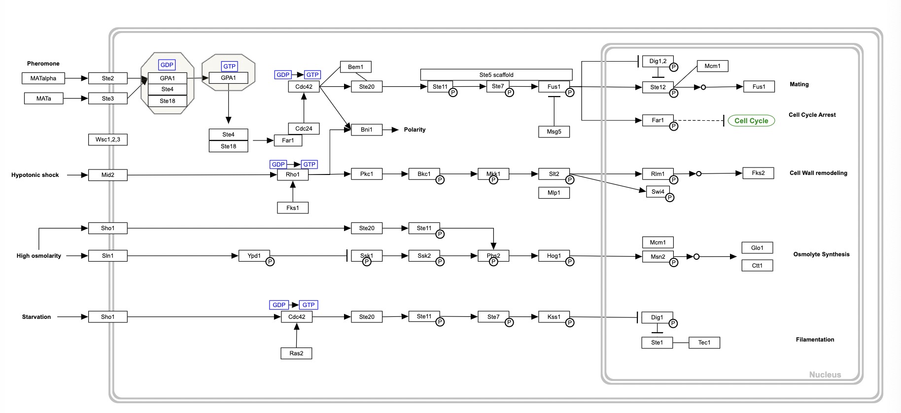
Figure 1: MAPK signaling pathway (Saccharomyces cerevisiae) from Wikipedia

The proposed methodology is applied to the z-scale data after imputation of missing value and transform to standard normal. Combining the initial clustering results with the diagnostic results from the heatmap, there are 4 small homogeneous groups. For variables that are mostly negatively correlated with other variables within the groups, we re-orient them by changing the sign such that the correlations within each group are positive.

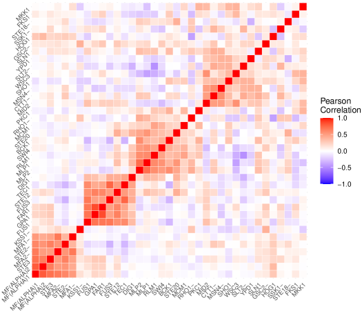
Figure 2: Heatmap of the yeast RNA expression data converted to normal scales; there are four homogeous groups from the bottom left to upper right, the group sizes are 7, 7, 9, 8 respectively. There are 6 isolated variables not in the 4 groups.

For each group, we introduce the proxy variables in (5) even though the group sizes $d_{g}$ are not large. The proxy variables are referred to as proxy1, proxy2, proxy3 and proxy4. The resulting vine dependency graph is shown in Figure 3.

Compare the vine dependency graph with the ground-truth figure, the genes linked to proxy1 and proxy2, such as MAT-$\alpha$, GPA1, DIG1, FAR1; they are closely related and are involved for cell cycle arrest process. A group of genes, such as SLN1, SHO1, YPD1, CTT1, are linked to the proxy4, and these genes are involved in “osmolyte synthesis process”. Another group of genes, RHO1, BKC1, SWI4, SLT2, and RLM1, are linked to the proxy3, and they are involved in “cell wall modelling process”. These findings suggest the links between the proxy variable and the observed variables could provide some group information and the genes clustered in the same group are usually involve in the same cell process.

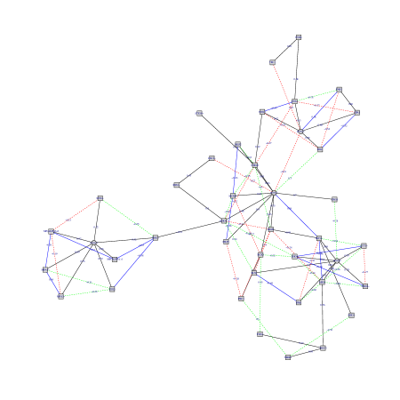
Figure 3: Vine dependency graphs for yeast RNA expression data; Edges in black from a maximal spanning tree and the connected edges in blue, red, and green explain the conditional dependence of variables given one, two and 3 or more variables. The edges are drawn in the plot if the partial correlation of two variables given one, two and three or more variables are greater than 0.25, 0.15, and 0.30 respectively and are labelled if they are greater than 0.5, 0.3, 0.4 respectively. The labels on the spanning tree in color black is the correlation between two variables while the labels on additional edges are partial correlation of variables given other variables. There are four proxy variables introduced (shown in circles) and the observed variables are shown in rectangles.

In addition to the group information, there are some interesting links in the vine dependency graph matches the ground-truth pathway graph in Figure 1. For example, in the cell wall remodelling process, the genes involved in the process are all linked closely in the vine graph: SLT2 linked to RLM1 in the first tree and linked to SWI4 through RML1. This matches with the path SLT2 $\longrightarrow$ RLM1 and SWI4 in the ground-truth pathway. A group of genes, PKC1, BCK1, proxy3 and RHO1 are linear in the first tree 1; this roughly matches the ground-truth path RHO1 $\longrightarrow$ PKC1 $\longrightarrow$ BCK1. Furthermore, the genes with many links to the other genes may act as hub genes and involve in multiple processes. For example, STE20 appears in multiple locations in Figure 1, and plays roles in multiple cell process. From the vine dependency graph, it also has many links within two edges to other genes in different groups.

4.2 Constructing condition-specific dependency networks in Prostate Cancer Study

We collected gene expression data profiled by RNA-sequencing over $n=497$ prostate adenocarcinoma patients in the cancer genome atlas (TCGA) cohort. RNA-sequencing technology directly measures the number of short reads mapped onto each gene (exons), which shows robust correlations with the number of mRNA molecules transcribed within each gene. Here, we specifically focus on genes previously known to be involved in the cancer developmental process (KEGG), as was done in the previous analysis [21]. For the selected 314 genes available in the TCGA data, and overlapping with the KEGG cancer pathway annotation, we applied our proposed methodology.

The CLV clustering algorithm partitioned the total 314 genes into six homogeneous groups, consisting of 55, 44, 63, 62, 44, and 46 variables. In order to estimate 1-factor models, we identified a total of 44 weakly-correlated variables, 3, 6, 5, 15, 8 and 7 from these six clusters and separated them out from each cluster, resulting in the tightly-connected groups of 52, 38, 58, 47, 36, and 39 variables largely explained by a single latent factor within each group.

For simpler illustration purpose (less busy graphs), we show the connected sub-graph constructed from the CLV-groups with index 1, 6, 3 which have more between group dependence. For groups 1, 6, 3, the numbers of variables used for proxy calculations were respectively 52, 39, 45. The vine dependency graph for all 6 groups in the additional file 1.

From the correlation matrix, some genes have RNA-seq values that are mostly negatively correlated with RNA-seq values of other genes. For these genes, we change the sign of the RNA-seq value in the z-scale; equivalently this is negation of the original RNA-seq values. A $-$ (minus sign) is added to the gene name for the heatmap and vine graphs.

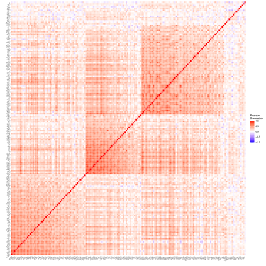
Figure 4: A gene expression correlation matrix between 164 genes computed on prostate cancer tumor samples. The color and intensity represent Pearson’s correlation values ($-1$ and $1$) based on normalized gene expression z-scores. From the bottom left to the right, the first block has 52 genes in group 1, the second block has 39 genes in group 6, and the third block has 58 genes in group 3. After third group, there are 15 genes separated out of the CLV groups.

In Figure 4, there are three homogeneous groups among the 164 genes and we denote the groups along the diagonal from the bottom left to be group 1, group 6 and group 3, and then 15 isolated genes separated from these CLV groups.

For the three groups, the enrichment analysis is performed on each group. The R package goseq is used to identify the ontology of the three groups and the top three potential ontology for each group are shown in Table 2.

group	ontopology
1	positive regulation of peptide hormone secretion
	drug metabolic process
	generation of precursor metabolites and energy
6	collagen-containing extracellular matrix
	angiogenesis
	skeletal system development
3	regulation of muscle system process
	nuclear lumen
	nucleoplasm

Table 2: The top 3 ontologies for the CLV-groups 1, 6, 3 .

Vine dependency graphs

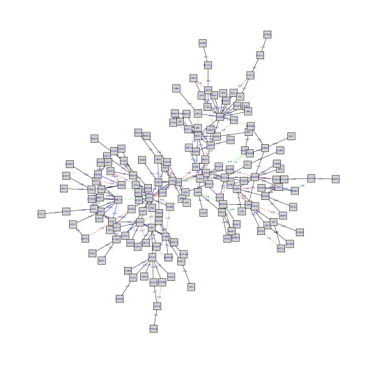
Figure 6: dependency graph for 164 genes in the RNA-seq data of prostate cancer. Edges in black from a maximal spanning tree and the connected edges in blue, red, and green explain the conditional dependence of variables given one, two and 3 or more variables. The edges are drawn in the plot if the absolute partial correlation of two variables given one, two and three or more variables are greater than 0.30, 0.15, and 0.30 respectively and are labelled if they are greater than 0.5, 0.3, 0.4 respectively. The labels on the spanning tree in color black is the correlation between two variables while the labels on additional edges are partial correlation of variables given other variables. There are no proxy variables introduced and the observed variables are shown in rectangles.

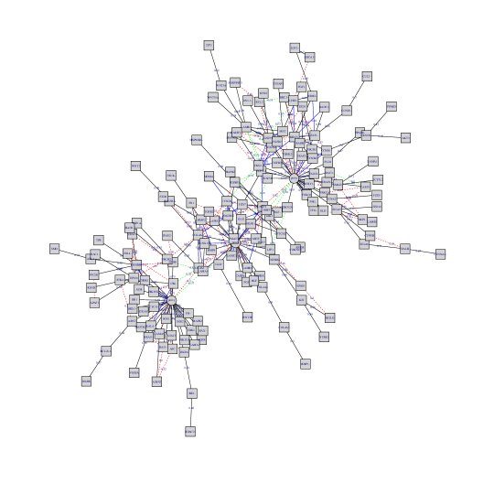
Figure 7: dependency graph for 164 genes in the RNA-seq data of prostate cancer with three proxy variables. Edges in black from a maximal spanning tree and the connected edges in blue, red, and green explain the conditional dependence of variables given one, two and 3 or more variables. The edges are drawn in the plot if the absolute partial correlation of two variables given one, two and three or more variables are greater than 0.30, 0.15, and 0.30 respectively and are labelled if they are greater than 0.5, 0.3, 0.4 respectively. The labels on the spanning tree in color black is the correlation between two variables while the labels on additional edges are partial correlation of variables given other variables. There are no proxy variables introduced and the observed variables are shown in rectangles.

For the tumor cases, vine dependency graphs were obtained without and with introducing the proxy variables; they are in Figures 6 and 7 respectively.

The simple thresholding on elements of the partial correlations in (2) are also performed to get conditional independency graphs. The summary statistics on the partial correlations are minimum: -0.34, 1st Quartile: -0.04, Median: 0.00, 3rd Quartle: 0.05, maximum: 0.77. Most of the partial correlation are small in absolute value and close to zero. The node degrees distributions for inferred networks for truncated vines and conditional independency graphs based on different thresholds 0.1 and 0.15 respectively are shown in Figure 5. In looking at genes with the largest node degrees and their neighbors, the resulting subsets are not related to the gene groups based on our methodology. [21] include several methods for producing graphs based on the inverse covariance matrix; however, we cannot match the tuning parameters of the methods to thresholds on partial correlations so we cannot make comparisons.

Based on the vine dependency graphs, we identify the most connected genes and summarize the results in Table 3. In the table, we also show the effect size of these genes computed from the raw RNA-seq counts in log scale and the logFC value (log of fold change) obtained from the DEG (differential expressed gene analysis) using R package edgeR. The fold change describes the differences of RNA expression in gene between normal and tumored cases. The positive fold changes are up-regulated and negative fold changes are down-regulated genes compared to the normal cases. In addition, all the genes in the table pass the tests for determining differential expression using the likelihood ratio test in edgeR, when the cut-off p-value is set at 0.05.

Figure 5: Node degree distributions for inferred networks for considered methods.

Table 3: The genes which pass the DEG test (perform LRT test using package “edgeR”; p-value cut off 0.05) and also have large number of links in the built vine dependency graphs. The panel shows the hub genes from the vine graphs built on the tumor samples; the left panel is for vine built without the proxies while the right panel is for vine built with introducing the proxies. effect size is computed in the log-scale: $(\overline{\log y}_{\text{tumor}}-\overline{\log y}_{\text{normal}})/s_{\text{pooled}}$, $y$ is the raw RNA-seq data, logFC denotes the log transform of fold-change which is defined as the ratio of ‘expression level’ in two groups. Proxy1, proxy6, proxy3 are for groups 1, 6, 3. For gene names ending with $-$, their RNA-seq values were re-oriented for drawing the heatmap and vine graphs.

gene(node-degree)	effect size	logFC	gene(node-degree)[group]	effect size	logFC
TCF7L1(18)	-1.81	-0.86	proxy3(33)	-	-
CREBBP(16)	-0.27	0.23	proxy1(32)	-	-
RBX1-(11)	0.43	0.63	proxy6(28)	-	-
LAMA4(10)	-0.86	-0.45	COL4A2 (14) [B]	-0.78	-0.51
BIRC5-(10)	1.74	2.33	GSTP1(12) [C]	-2.04	-1.87
ITGB1(9)	-1.28	-0.51	BIRC5-(11) [C]	1.74	2.33
FGFR1(9)	-1.10	-0.54	FGF2(9) [B]	-1.19	-0.61
FZD7(9)	-1.21	-0.64	TCF7L1(9) [C]	-1.81	-0.86
GSTP1(9)	-2.04	-1.87	CREBBP(9) [A]	-0.27	0.23
COL4A2(8)	-0.78	-0.51	LAMB3(9) [C]	-1.28	-1.42
FGF2(8)	-1.19	-0.61	E2F1-(8) [C]	0.90	1.36
EP300(7)	-0.25	0.26	MMP2(7) [B]	-0.73	-0.26
LAMB3(8)	-1.28	-1.42	CKS2-(7) [C]	0.85	1.11
TGFBR2(8)	-1.05	-0.46	CBL(7) [A]	-0.42	0.15
ITGA3(8)	-1.45	-0.67	-	-	-
HRAS-(7)	0.30	0.52	-	-	-
GTSE1-(7)	1.70	2.02	-	-
RRM2-(7)	1.79	1.94	-	-	-
E2F1-(7)	0.90	1.36	-	-	-
CHEK2-(7)	1.06	1.04	-	-	-

From the two vine dependency graphs, isolated variables usually have node degree 1, and these are far from the clusters connected around the proxy variables. The genes used to calculate the proxy variables are usually directly linked to the corresponding group-based proxy variable, while some of them are linked via a secondary tree to the proxy variable through one of the other genes in that group.

The hub genes are usually strongly correlated with the proxy variable in the group and also have a relatively strong correlation with other variables in the group. Examples are genes BIRC5, GSTP1, TCF7L1, CREBBP; they are linked to a proxy variable and are connected to other variables in a star shape. Some hub genes such as FGF2 connect to proxy variables in one group and also to genes in another group, acting as a bridge between the two groups. Another example for bridging is the gene COL4A2; it connects to the proxy variables of the group 6 and to the genes of group 1. LAMB3 is a gene from group 3, but was not used to calculate the proxy variable because it shows strong residual dependence. The graph shows that this gene is linked to multiple groups. The links with genes in group 3 explains the residual local dependence after taking into account the group effect, while the links with the group 6 proxy variable through the gene TCF7L1 explain between-group dependence (and non-weak residual dependence).

From Table 3, there are several hub genes (with “$-$” after the gene name) that are re-oriented because negative correlation of RNA-seq values with those of many other genes; examples are RBX1, BIRC5, E2F1. The effect size of these genes are positive, which indicates they are up-regulated in the prostate cancer patients relative to non-diseased subjects. The RNA-seq variables that were not re-oriented had mainly negative effect sizes, indicating that the corresponding genes are down-regulated in prostate cancer patients.

Combining the two vine dependency graphs with Table 3, we expect the most connected genes with a relatively large effect size may play an important role in the development of the prostate cancer. A shortlist of hub genes in tumor patients consists of COL4A2, GSTP1, BIRC5, FGF2, TCF7L1, CREBBP, LAMB3, E2F1 from the vine graphs with proxies, and the most connected genes with large effect size are RBX1, LAMA4, ITGB1, FGFR1, FZD7, EP300, TGFBR2 in the vine graphs without proxies.

For those potential hub genes, some of them have some related biological evidence to support them.

• TCF7L1: [31] suggest that induction of WNT4/TCF7L1 results in increased NED and malignancy in prostate cancer that is linked to dysregulation of androgen receptor signaling and activation of the IL-8/CXCR2 pathway.

• BIRC5: BIRC5 is an immune-related gene that inhibits apoptosis and promotes cell proliferation. It is highly expressed in most tumors and leads to poor prognosis in cancer patients. [33] shows BIRC5 was significantly correlated with multiple immune cells infiltrates in a variety of tumors.

• GSTP1: [25] states the gene belongs to the GSTs family, a group of enzymes involved in detoxification of exogenous substances and it also plays an important role in cell cycle regulation. Its dysregulation correlates with a large variety of tumors, in particular with prostate cancer.

• FGF2: From [12] and [27], Fibroblast growth factor (FGF) 2 (or basic FGF) is expressed at increased levels in human prostate cancer. FGF2 can promote cell motility and proliferation, increase tumor angiogenesis, and inhibit apoptosis, all of which play an important role in tumor progression. Recently, [22] also identifies the FGF2 gene as a hub gene in the development of the prostate cancer.

Based on all the biological evidence, the hub genes we identified from the small subset (164 genes) play important roles in the progression of prostate cancer; this indicates that the vine dependency graphs can provide some interesting and useful insights.

5 Discussion

This paper presents a method to construct dependency graphs via truncated vines with latent variables. It makes use of low-order partial correlations and avoids the problem of high-order partial correlations used in conditional dependency graphs. Low-order partial correlations are easier to interpret for the conditional dependence between variables. With latent variables that can explain much of the dependence in groups of variables, high-order partial correlations get closer to 0 in absolute value as the number of varables linked to each latent variable increases.

Here we address the problem of finding a specialized from of dependency structures from data while constraining candidate graphs to be a vine graph. Finding a statistical dependency network from observed data has long been of great interest to computational biologists since the first introduction of microarray technology to date. However, structural learning over combinatorial spaces of general graphs, such as directed acyclic graphs (DAG), makes exact latent structure inference highly intractable and resorts to greedy optimization algorithms [11]. Even if we could enumerate all of these structures, given the limited sample size of expression data, a scoring function (objective) often run into a critical problem of distinguishing multiple equally, or at least similarly, likely structures [6]. However, interpretable truncated vine structures can be obtained with a relatively smaller data set.

Statistical dependency structures generally do not correspond to physical protein-protein interaction networks; hence, care should be taken for biological interpretations. Instead, dependency maps typically represent the notion of functional modules, and hub nodes (high-degree vertices) implicate essential genes that participate in multiple biological processes. Modeling statistical dependency structures over high-dimensional gene expression data also benefits subsequent analysis. For instance, conditional probability calculation facilitated by a vine graph (conditional independency structures) will improve regression and classification problems in predicting the outcome of diseases based on observed gene expressions [[10], [8]]. We could also expect our approach will provide an efficient way to compute marginal probabilities over many genes thanks to the sparsity by construction. This is particularly appealing for G-formula computation in causality inference [26].

References

- [1] T. W. Anderson. An Introduction to Multivariate Statistical Analysis. Wiley, New York, 1958.
- [2] A.-L. Barabasi and Z. N. Oltvai. Network biology: understanding the cell’s functional organization. Nature Reviews Genetics, 5(2):101–113, 2004.
- [3] T. Bedford and R. M. Cooke. Vines–a new graphical model for dependent random variables. Annals of Statistics, 30(4):1031–1068, 2002.
- [4] E. C. Brechmann and H. Joe. Truncation of vine copulas using fit indices. Journal of Multivariate Analysis, 138:19–33, 2015.
- [5] R. B. Brem, G. Yvert, R. Clinton, and L. Kruglyak. Genetic dissection of transcriptional regulation in budding yeast. Science, 296(5568):752–755, 2002.
- [6] D. M. Chickering. Learning equivalence classes of Bayesian-Network structures. The Journal of Machine Learning Research, 2:445–498, 2002.
- [7] C. Chow and C. Liu. Approximating discrete probability distributions with dependence trees. IEEE transactions on Information Theory, 14(3):462–467, 1968.
- [8] H.-Y. Chuang, E. Lee, Y.-T. Liu, D. Lee, and T. Ideker. Network-based classification of breast cancer metastasis. Molecular Systems Biology, 3(1):140, 2007.
- [9] X. Fan and H. Joe. High-dimensional factor copula models with estimation of latent variables. arXiv preprint arXiv:2205.14487, 2022.
- [10] N. Friedman, D. Geiger, and M. Goldszmidt. Bayesian Network classifiers. Machine Learning, 29(2):131–163, 1997.
- [11] N. Friedman, M. Linial, I. Nachman, and D. Pe’er. Using Bayesian Networks to analyze expression data. Journal of Computational Biology, 7(3-4):601–620, 2000.
- [12] D. Giri, F. Ropiquet, and M. Ittmann. Alterations in expression of basic Fibroblast Growth Factor (FGF) 2 and its receptor FGFR-1 in human prostate cancer. Clinical Cancer Research, 5(5):1063–1071, 1999.
- [13] R. Jansen, D. Greenbaum, and M. Gerstein. Relating whole-genome expression data with protein-protein interactions. Genome Research, 12(1):37–46, 2002.
- [14] H. Joe. Dependence Modeling with Copulas. Chapman & Hall/CRC, Boca Raton, FL, 2014.
- [15] H. Joe. Parsimonious graphical dependence models constructed from vines. Canadian Journal of Statistics, 46(4):532–555, 2018.
- [16] M. Kanehisa, S. Goto, M. Furumichi, M. Tanabe, and M. Hirakawa. KEGG for representation and analysis of molecular networks involving diseases and drugs. Nucleic Acids Research, 38(suppl_1):D355–D360, 2010.
- [17] T. Kelder, M. P. Van Iersel, K. Hanspers, M. Kutmon, B. R. Conklin, C. T. Evelo, and A. R. Pico. WikiPathways: building research communities on biological pathways. Nucleic Acids Research, 40(D1):D1301–D1307, 2012.
- [18] P. Krupskii and H. Joe. Approximate likelihood with proxy variables for parameter estimation in high-dimensional factor copula models. Statistical Papers, 63:543–569, 2022.
- [19] D. Kurowicka and R. Cooke. A parameterization of positive definite matrices in terms of partial correlation vines. Linear Algebra and its Applications, 372:225–251, 2003.
- [20] D. Kurowicka and R. M. Cooke. Uncertainty analysis with high dimensional dependence modelling. Wiley, Chichester, 2006.
- [21] L. Lin, M. Drton, and A. Shojaie. Estimation of high-dimensional graphical models using regularized score matching. Electronic Journal of Statistics, 10(1):806, 2016.
- [22] S. Liu, W. Wang, Y. Zhao, K. Liang, and Y. Huang. Identification of potential key genes for pathogenesis and prognosis in prostate cancer by integrated analysis of gene expression profiles and the cancer genome atlas. Frontiers in Oncology, 10:809, 2020.
- [23] E. Z. Macosko, A. Basu, R. Satija, J. Nemesh, K. Shekhar, M. Goldman, I. Tirosh, A. R. Bialas, N. Kamitaki, E. M. Martersteck, et al. Highly parallel genome-wide expression profiling of individual cells using nanoliter droplets. Cell, 161(5):1202–1214, 2015.
- [24] P. M. Magwene and J. Kim. Estimating genomic coexpression networks using first-order conditional independence. Genome Biology, 5(12):1–16, 2004.
- [25] F. Martignano, G. Gurioli, S. Salvi, D. Calistri, M. Costantini, R. Gunelli, U. De Giorgi, F. Foca, and V. Casadio. GSTP1 methylation and protein expression in prostate cancer: diagnostic implications. Disease Markers, 2016.
- [26] A. I. Naimi, S. R. Cole, and E. H. Kennedy. An introduction to g methods. International Journal of Epidemiology, 46(2):756–762, 2017.
- [27] N. Polnaszek, B. Kwabi-Addo, L. E. Peterson, M. Ozen, N. M. Greenberg, S. Ortega, C. Basilico, and M. Ittmann. Fibroblast Growth Factor 2 promotes tumor progression in an autochthonous mouse model of prostate cancer. Cancer Research, 63(18):5754–5760, 2003.
- [28] M. Schena, D. Shalon, R. W. Davis, and P. O. Brown. Quantitative monitoring of gene expression patterns with a complementary DNA microarray. Science, 270(5235):467–470, 1995.
- [29] E. Vigneau and E. Qannari. Clustering of variables around latent components. Communications in Statistics-Simulation and Computation, 32(4):1131–1150, 2003.
- [30] Z. Wang, M. Gerstein, and M. Snyder. RNA-Seq: a revolutionary tool for transcriptomics. Nature Reviews Genetics, 10(1):57–63, 2009.
- [31] Y.-C. Wen, Y.-N. Liu, H.-L. Yeh, W.-H. Chen, K.-C. Jiang, S.-R. Lin, J. Huang, M. Hsiao, and W.-Y. Chen. TCF7L1 regulates cytokine response and neuroendocrine differentiation of prostate cancer. Oncogenesis, 10(11):1–11, 2021.
- [32] J. Whittaker. Graphical Models in Applied Multivariate Statistics. Wiley, Chichester, 1990.
- [33] L. Xu, W. Yu, H. Xiao, and K. Lin. BIRC5 is a prognostic biomarker associated with tumor immune cell infiltration. Scientific Reports, 11(1):1–13, 2021.