A Slightly Lifted Convex Relaxation
for Nonconvex Quadratic Programming
with Ball Constraints

Abstract

Globally optimizing a nonconvex quadratic over the intersection of $m$ balls in $\mathbb{R}^{n}$ is known to be polynomial-time solvable for fixed $m$. Moreover, when $m=1$, the standard semidefinite relaxation is exact. When $m=2$, it has been shown recently that an exact relaxation can be constructed using a disjunctive semidefinite formulation based essentially on two copies of the $m=1$ case. However, there is no known explicit, tractable, exact convex representation for $m\geq 3$. In this paper, we construct a new, polynomially sized semidefinite relaxation for all $m$, which does not employ a disjunctive approach. We show that our relaxation is exact for $m=2$. Then, for $m\geq 3$, we demonstrate empirically that it is fast and strong compared to existing relaxations. The key idea of the relaxation is a simple lifting of the original problem into dimension $n+1$. Extending this construction: (i) we show that nonconvex quadratic programming over $\|x\|\leq\min\{1,g+h^{T}x\}$ has an exact semidefinite representation; and (ii) we construct a new relaxation for quadratic programming over the intersection of two ellipsoids, which globally solves all instances of a benchmark collection from the literature.

1 Introduction

We study the nonconvex optimization problem

$$\min_{x\in\mathbb{R}^{n}}\left\{x^{T}Qx+2\,q^{T}x:\begin{array}[]{l}\|x-c_{i}\|\leq\rho_{i}\quad\forall\ i=1,\ldots,m\end{array}\right\},$$ (QP)

where the data are the $n\times n$ symmetric matrix $Q$, column vectors $q,c_{1},\ldots,c_{m}\in\mathbb{R}^{n}$, and positive scalars $\rho_{1},\ldots,\rho_{m}\in\mathbb{R}$. In words, (QP) is nonconvex quadratic programming over the intersection of $m$ balls in $n$-dimensional space. Without loss of generality, we assume $c_{1}=0$ and $\rho_{1}=1$, i.e., the first constraint is the unit ball. Note that, while the feasible set of (QP) is convex, the objective function is generally nonconvex since $Q$ is not necessarily positive semidefinite. We assume that (QP) is feasible and hence has an optimal solution, and we are specifically interested in strong convex relaxations of (QP).

Although (QP) is polynomial-time solvable to within $\epsilon$-accuracy for fixed $m$ [6], there is no known exact convex relaxation for all $m$. By exact, we mean a relaxation with optimal value equal to that of (QP). When $m=1$, the standard semidefinite (SDP) relaxation is exact [22]. This relaxation is often called the Shor relaxation and involves a single $(n+1)\times(n+1)$ positive semidefinite variable. For $m=2$, Kelly et al. [19] have recently shown that a particular disjunctive semidefinite relaxation is exact. Their construction is based on essentially two copies of the $m=1$ case, and as a result, it utilizes two $(n+1)\times(n+1)$ positive semidefinite variables. These and other SDP relaxations are detailed in Section 2. Our goals in this paper are: (i) to construct a new, strong, non-disjunctive SDP relaxation, which is polynomially sized in $n$ and $m$; (ii) to prove its exactness for $m=2$; and (iii) to demonstrate empirically its effectiveness for larger $m$. In particular, by non-disjunctive, we mean that the SDP optimizes over just one semidefinite variable like the Shor relaxation—but with additional constraints on that matrix variable.

Another line of research examines conditions on the data of (QP) under which the Shor relaxation is exact. Note that, without loss of generality, by an orthogonal rotation in the $x$ space, $Q$ may be assumed to be diagonal. In this case, (QP) is a special case of a diagonal quadratically constrained quadratic program (diagonal QCQP), that is, a QCQP in which every quadratic function has a diagonal Hessian. Diagonal QCQPs are well studied in the literature [12, 13, 20, 26, 4], where it is known, for example, that the Shor relaxation of (QP) is exact if $\text{sign}(q_{j})=-\text{sign}(c_{1j})=\cdots=-\text{sign}(c_{mj})$ for all $j=1,\ldots,n$ [24]. In this paper, however, we seek a relaxation that is strong irrespective of the data.

(QP) can also be optimized globally using any of the high-quality global-optimization algorithms and software packages available today. We are also aware of several papers studying global approaches for (QP) that take into account the problem’s specific structure [7, 5, 1]. Each of these papers uses some combination of enumeration and lower bounding to find a global optimal solution and verify its optimality. In contrast, we are interested in computing a single strong bound ( exact for $m=2$, as mentioned above), and we will show that for $m\geq 3$ our relaxation is frequently strong enough to deliver a global optimal solution via a rank-1 SDP optimal solution. Moreover, our relaxation could certainly be used as the lower-bounding technique within an enumerative scheme to optimize (QP) globally, but we leave this for future research.

As we began this project, we were motivated by the idea of constructing an exact relaxation for (QP) for all $m$. Given that (QP) is only known to be polynomial-time for fixed $m$—not as a function of $m$—it was unclear whether a given relaxation, which is polynomial in $m$, could possibly be exact for all $m$. Ultimately, we will show that our relaxation is exact for $m=2$ but inexact for $m\geq 3$; see Section 3.4. Even still, we believe that our new relaxation makes significant progress towards approximating (QP) for larger $m$ as we demonstrate empirically.

Our approach is based on two simple transformations of the feasible set of (QP). First, we write the feasible set in the equivalent form

$$\left\{x\in\mathbb{R}^{n}:x^{T}x\leq\rho_{i}^{2}-c_{i}^{T}c_{i}+2c_{i}^{T}x\quad\forall\ i=1,\ldots,m\right\}.$$

Note that the $i$-th constraint is representable using a rotated second-order-cone constraint of size $n+2$. Second, we insert an auxiliary variable $\beta\in\mathbb{R}$ within each constraint:

$$\left\{{x\choose\beta}\in\mathbb{R}^{n+1}:\begin{array}[]{l}x^{T}x\leq\beta\\ \beta\leq\rho_{i}^{2}-c_{i}^{T}c_{i}+2c_{i}^{T}x\quad\forall\ i=1,\ldots,m\end{array}\right\}.$$

Here, $\beta\leq\rho_{i}^{2}-c_{i}^{T}c_{i}+2c_{i}^{T}x$ is a linear constraint in $x$ and $\beta$. We can then equivalently minimize $x^{T}Qx+2q^{T}x$ over feasible ${x\choose\beta}\in\mathbb{R}^{n+1}$. The intuition for these transformations comes from the fact that we are exchanging $m-1$ cone constraints in the original problem with $m$ linear constraints. In this sense, we have greatly simplified the structure of the feasible set.

The paper is organized as follows. In Section 2, we introduce the required background necessary to build and evaluate SDP relaxations of (QP). We also discuss the literature on relaxations specifically for (QP), including the exact relaxations mentioned above when $m=1$ and $m=2$. Then, in Section 3, we introduce our new relaxation, which we show to be exact for $m=2$ and empirically quite tight for $m\geq 3$. (The proof for $m=2$ is relegated to Section 5.) Next, Section 4 considers two extensions. First, we study the related problem of nonconvex quadratic programming over the set

$$\left\{x\in\mathbb{R}^{n}:\begin{array}[]{l}\|x\|\leq 1\\ \|x\|\leq g+h^{T}x\end{array}\right\},$$

i.e., when linear functions bound the norm of $x$ instead of the squared norm. This is an interesting case in its own right, arising for example as a substructure in the optimal power flow problem [14, 17] and also studied by Kelly et al. [19]. Second, we extend our method to nonconvex quadratic programming over the intersection of two general ellipsoids, which is known as the Celis-Dennis-Tapia problem or the two trust-region subproblem (TTRS). See [15] and references therein for recent work on TTRS. We show empifically that our approach solves all instances of a test set from the literature. Finally, Section 5 contains the proof of our main exactness result from Section 3.

We remark that all computational results in the paper were coded in Python using the Fusion API of MOSEK 10.0.37 [3] and run on a M2 MacBook Air with 24 GB of RAM. Source code, scripts, and results are available at https://github.com/sburer/ballconstraints.

1.1 Notation and terminology

Our notation and terminology is mostly standard. $\mathbb{R}^{d}$ is the space of $d$-dimensional real column vectors, and $\mathbb{S}^{d}$ is the space of $d\times d$ real symmetric matrices. The identity matrix in $\mathbb{S}^{d}$ is denoted $I_{d}$, and the trace inner product on $\mathbb{S}^{d}$ is defined as $M\bullet N:=\text{trace}(MN)$ for any two matrices $M,N\in\mathbb{S}^{d}$. Define

$$\mathcal{SOC}^{d} :=\left\{v\in\mathbb{R}^{d}:\|(v_{2},\ldots,v_{d})\|\leq v_{1}\right\},$$

$${\color[rgb]{0,0,0}\mathcal{RSOC}^{d}} :={\color[rgb]{0,0,0}\left\{v\in\mathbb{R}^{d}:v_{3}^{2}+\cdots+v_{d}^{2}\leq 2v_{1}v_{2},\ v_{1}\geq 0,\ v_{2}\geq 0\right\}},$$

$$\mathcal{PSD}^{d} :=\left\{M\in\mathbb{S}^{d}:M\text{ is positive semidefinite}\right\}$$

to be the $d$-dimensional second-order cone, the $d$-dimensonal rotated second-order cone, and the $d\times d$ positive semidefinite cone, respectively. It is well known that

$$T_{d}\,\mathcal{RSOC}^{d}=\mathcal{SOC}^{d},\quad\text{where}\quad T_{d}:=\begin{pmatrix}1/\sqrt{2}&1/\sqrt{2}&0\\ 1/\sqrt{2}&-1/\sqrt{2}&0\\ 0&0&I_{d-2}\end{pmatrix}\in\mathcal{S}^{d\times d},$$

that is, $\mathcal{RSOC}^{d}$ is the image of $\mathcal{SOC}^{d}$ under the orthogonal rotation given by $T_{d}$. We use SOC and PSD as abbreviations for second-order cone and positive semidefinite. For any cone $S$, its conic hull is defined as all finite sums of members in $S$, i.e., $\operatorname{conic.hull}({\color[rgb]{0,0,0}S}):=\{\sum_{k=1}^{K}s_{k}:K\in\mathbb{N},s_{k}\in S\}$.

2 Background on Semidefinite Relaxations

In this section, we recount techniques and constructions from the literature, which we will use for building convex relaxations in Section 3. We also detail prior research on relaxations of (QP) specifically. Finally, we discuss standard ways to measure the quality of a given relaxation on a particular problem instance, which will be employed in Sections 3–4.

We caution the reader that we will reuse (or “overload”) some notation in this section. For example, the variable $x$ and dimension $n$ in this section are not strictly the same as defined in the Introduction.

2.1 Techniques for building an SDP relaxation

For this subsection as well as Section 2.3, we introduce the generic nonconvex quadratic programming problem

$$\min\left\{x^{T}Qx:x\in\mathcal{K},\ x_{1}=1\right\},$$ (1)

where

$$\mathcal{K}:=\left\{x\in\mathbb{R}^{n}:\begin{array}[]{l}\ell_{1}^{T}x\geq 0,\ \ell_{2}^{T}x\geq 0\\ L_{3}^{T}x\in\mathcal{SOC}^{d_{3}},\ L_{4}^{T}x\in\mathcal{SOC}^{d_{4}}\end{array}\right\}$$

is a closed, convex cone with polyhedral and second-order-cone constraints defined by the data vectors $\ell_{1},\ell_{2}\in\mathbb{R}^{n}$ and data matrices $L_{3}\in\mathbb{R}^{n\times d_{3}},L_{4}\in\mathbb{R}^{n\times d_{4}}$. Specifically, $\mathcal{K}$ is defined by two linear constraints and two SOC constraints of different sizes. We assume that $\{x\in\mathcal{K}:x_{1}=1\}$ is nonempty and bounded in which case (1) has an optimal solution. We also assume that the constraints defining $\mathcal{K}$ imply $x_{1}\geq 0$.

It is well known that (1) is equivalent to

$$\min\left\{Q\bullet X:X\in\mathcal{H},\ X_{11}=1\right\},$$ (2)

where

$$\mathcal{H}:=\operatorname{conic.hull}\left\{X=xx^{T}:x\in\mathcal{K}\right\}\subseteq\mathbb{S}^{n}.$$

Equivalent means that both have the same optimal value and there exists a rank-1 optimal solution $X^{*}=x^{*}(x^{*})^{T}$ of (2), where $x^{*}$ is optimal for (1). Hence, a common approach to optimize or approximate (1) is to build strong convex relaxations of $\mathcal{H}$, and in particular, semidefinite relaxations are a typical choice.

One standard option is the Shor relaxation of $\mathcal{H}$:

$$\text{\text{\sc Shor}}:=\left\{X\in\mathcal{PSD}^{n}:\begin{array}[]{l}Xe_{1}\in\mathcal{K}\\ J_{d_{3}}\bullet L_{3}^{T}XL_{3}\geq 0\\ J_{d_{4}}\bullet L_{4}^{T}XL_{4}\geq 0\end{array}\right\},$$

where $e_{1}\in\mathbb{R}^{n}$ is the first unit vector and, for any dimension $d$,

$$J_{d}:=\begin{pmatrix}1&0\\ 0&-I_{d-1}\end{pmatrix}\in\mathbb{S}^{d}.$$

Here, $Xe_{1}\in\mathcal{K}$ reflects the constraint $x\in\mathcal{K}$ of (1) and is derived from the implications

$$x\in\mathcal{K}\quad\Longrightarrow\quad x_{1}\geq 0\quad\Longrightarrow\quad x_{1}x\in\mathcal{K}\quad\Longrightarrow\quad Xe_{1}\in\mathcal{K}$$

where $e_{1}$ is the first standard unit vector. Morevover, the linear constraint $J_{d_{k}}\bullet L_{k}^{T}XL_{k}\geq 0$ is derived from the quadratic function defining $L_{k}^{T}x\in\mathcal{SOC}^{d_{k}}$. The Shor relaxation with the constraint $X_{11}=1$ possesses an important property. When the objective matrix $Q$ is positive semidefinite on the subset of entries $x_{2},\ldots,x_{n}$ of $x$, then Shor is already strong enough to optimize the quadratic problem, i.e., the optimal value of (2) equals the optimal value of (1), and the embedded solution $Xe_{1}$ is optimal.

Next, we introduce an RLT constraint [23] using the implications

$$\ell_{1}^{T}x\geq 0,\ \ell_{2}^{T}x\geq 0\quad\Longrightarrow\quad\ell_{1}^{T}xx^{T}\ell_{2}\geq 0\quad\Longrightarrow\quad\ell_{1}^{T}X\ell_{2}\geq 0,$$

and SOCRLT constraints [25, 9] using

$$\ell_{i}^{T}x\geq 0,\ L_{k}^{T}x\in\mathcal{SOC}^{d_{k}}\quad\Longrightarrow\quad L_{k}^{T}xx^{T}\ell_{i}\in\mathcal{SOC}^{d_{k}}\quad\Longrightarrow\quad L_{k}^{T}X\ell_{i}\in\mathcal{SOC}^{d_{k}}.$$

Then defining

RLT $$:=\left\{X\in\mathbb{S}^{n}:\ell_{1}^{T}X\ell_{2}\geq 0\right\},$$

SOCRLT $$:=\left\{X\in\mathbb{S}^{n}:L_{k}^{T}X\ell_{i}\in\mathcal{SOC}^{d_{k}}\ \ \forall\ i=1,2,\ k=3,4\right\},$$

we arrive at the strengthened relaxation

$$\text{\sc Shor}\cap\text{\sc RLT}\cap\text{\sc SOCRLT}.$$

Another valid constraint can be derived from the fact that $L_{k}^{T}x\in\mathcal{SOC}^{d_{k}}$ is equivalent to a positive semidefinite constraint (or linear matrix inequality) [2]. We first write $y:=L_{3}^{T}x$ and $z:=L_{4}^{T}x$, so that the SOC constraints in (1) are $y\in\mathcal{SOC}^{d_{3}}$ and $z\in\mathcal{SOC}^{d_{4}}$. Then it is well-known that

$$y\in\mathcal{SOC}^{d_{3}}\quad\Longleftrightarrow\quad\operatorname{Arr}_{d_{3}}(y):=\begin{pmatrix}y_{1}&y_{2}&\cdots&y_{d_{3}}\\ y_{2}&y_{1}&&\\ \vdots&&\ddots&\\ y_{d_{3}}&&&y_{1}\end{pmatrix}\in\mathcal{PSD}^{d_{3}}.$$

For any dimension $d$, $\operatorname{Arr}_{d}:\mathbb{R}^{d}\to\mathbb{S}^{d}$ is called the arrow operator. Likewise $z\in\mathcal{SOC}^{d_{4}}$ if and only if $\operatorname{Arr}_{d_{4}}(z)\in\mathcal{PSD}^{d_{4}}.$ Then, using the fact that the Kronecker product of PSD matrices is PSD, we have $\operatorname{Arr}_{d_{3}}(y)\otimes\operatorname{Arr}_{d_{4}}(z)\in\mathcal{PSD}^{d_{3}d_{4}}$. Because the left-hand side of this expression is quadratic in $y$ and $z$, we can equivalently write

$$\operatorname{Arr}_{d_{3}}(y)\otimes\operatorname{Arr}_{d_{4}}(z)=(\operatorname{Arr}_{d_{3}}\boxtimes\operatorname{Arr}_{d_{4}})(zy^{T})$$

where $\operatorname{Arr}_{d_{3}}\boxtimes\operatorname{Arr}_{d_{4}}:\mathbb{R}^{d_{4}\times d_{3}}\to\mathbb{S}^{d_{3}d_{4}}$ is an operator that is linear in $zy^{T}$ and defined by

$$(\operatorname{Arr}_{d_{3}}\boxtimes\operatorname{Arr}_{d_{4}})(zy^{T}):=\begin{pmatrix}\operatorname{Arr}_{{\color[rgb]{0,0,0}d_{4}}}(y_{1}z)&\operatorname{Arr}_{{\color[rgb]{0,0,0}d_{4}}}(y_{2}z)&\cdots&\operatorname{Arr}_{{\color[rgb]{0,0,0}d_{4}}}(y_{d_{3}}z)\\ \operatorname{Arr}_{{\color[rgb]{0,0,0}d_{4}}}(y_{2}z)&\operatorname{Arr}_{{\color[rgb]{0,0,0}d_{4}}}(y_{1}z)&&\\ \vdots&&\ddots&\\ \operatorname{Arr}_{{\color[rgb]{0,0,0}d_{4}}}(y_{d_{3}}z)&&&\operatorname{Arr}_{{\color[rgb]{0,0,0}d_{4}}}(y_{1}z)\end{pmatrix}.$$

Substituting back $y=L_{3}^{T}x$ and $z=L_{4}^{T}x$, we arrive at the implication

$$(\operatorname{Arr}_{d_{3}}\boxtimes\operatorname{Arr}_{d_{4}})(L_{4}^{T}xx^{T}L_{3})\in\mathcal{PSD}^{d_{3}d_{4}}\quad\Longrightarrow\quad(\operatorname{Arr}_{d_{3}}\boxtimes\operatorname{Arr}_{d_{4}})(L_{4}^{T}XL_{3})\in\mathcal{PSD}^{d_{3}d_{4}}.$$

Then defining

$$\text{\sc Kron}:=\left\{X\in\mathbb{S}^{n}:(\operatorname{Arr}_{d_{3}}\boxtimes\operatorname{Arr}_{d_{4}})(L_{4}^{T}XL_{3})\in\mathcal{PSD}^{d_{3}d_{4}}\right\},$$

we have the strongest relaxation thus far:

$$\text{\sc Shor}\cap\text{\sc RLT}\cap\text{\sc SOCRLT}\cap\text{\sc Kron}.$$

In Section 3, we will derive SDP relaxations for (QP) using the building blocks just introduced, i.e., Shor combined with RLT, SOCRLT, and Kron. In a sense, each of the three relaxations RLT, SOCRLT, and Kron have the same goal—to combine information from pairs of constraints in (1)—but differ due to the structure of the underlying cones, i.e., the nonnegative orthant, the second-order cone, and the PSD cone.

2.2 Results from the literature

The relaxations Shor, RLT, SOCRLT, and Kron just introduced are known to be quite strong in a number of contexts closely related to (QP). Specifically, Shor is exact for the case of (QP) for $m=1$ [22], and when a single linear constraint is added to the ball constraint $\|x\|\leq 1$, then $\text{\sc Shor}\cap\text{\sc SOCRLT}$ is exact [25]. In addition, for the more general case

$$\left\{x:\begin{array}[]{l}\|x\|\leq 1\\ 0\leq g_{i}+h_{i}^{T}x\ \ \forall\ i=2,\ldots,m\end{array}\right\}$$

in which multiple linear constraints are added, $\text{\sc Shor}\cap\text{\sc RLT}\cap\text{\sc SOCRLT}$ is guaranteed to be exact when none of the hyperplanes $0=g_{i}+h_{i}^{T}x$ intersect inside the ball [11]. Kron has also been used to strengthen relaxations of (QP) when there is a second ellipsoidal constraint [2], not necessarily a ball; this is TTRS mentioned in the Introduction. As a footnote, we are unaware of any case in which enforcing Kron makes a relaxation exact for all objectives, but nevertheless Kron has proven to be a valuable tool for building strong relaxations.

We are aware of two papers [18, 17], which have studied techniques for further strengthening $\text{\sc Shor}\cap\text{\sc RLT}\cap\text{\sc SOCRLT}\cap\text{\sc Kron}$. Among these, [17] is more similar to the current paper. In [17], the authors introduce a class of linear cuts for SDP relaxations of

$$\{x:\|x\|\leq 1,\ \|x-c_{2}\|\leq g_{2}+h_{2}^{T}x\},$$

and they show how to separate the cuts in polynomial time. Through a series of computational experiments, the authors also show that their cuts are effective particularly in lower dimensions, say, for $n\leq 10$.

As mentioned in the Introduction, an exact convex relaxation of (QP) via a disjunctive formulation for the case $m=2$ was recently given by Kelly et al. [19]. They showed that the feasible region of (QP) can be written as the union of two special sets:

$$\{x:\|x\|\leq 1,\ 0\leq g_{1}+h_{1}^{T}x\}\quad\quad\text{and}\quad\quad\{x:\|x-c_{2}\|\leq\rho_{2},\ 0\leq g_{2}+h_{2}^{T}x\}.$$

Explicit formulas for $g_{i}$ and $h_{i}$ are given in their paper. Since optimizing over each of these can separately be accomplished with $\text{\sc Shor}\cap\text{\sc SOCRLT}$ as mentioned above, the authors then use a disjunctive formulation with two copies of $\text{\sc Shor}\cap\text{\sc SOCRLT}$ to derive an exact formulation of (QP); see proposition 5 in their paper. The authors also used similar ideas to derive an exact, disjunctive formulation for the case $\|x\|\leq\min\{1,g+h^{T}x\}$, a case we will also consider in Section 4.

Zhen et al. [28] have recently suggested another technique for combining information from two SOC constraints; see appendix B of [28]. We illustrate their idea using the two constraints $\|x\|\leq 1$ and $\|x-c_{2}\|\leq\rho_{2}$ of (QP). The fact that $\|uv^{T}\|_{2}=\|u\|\|v\|$, where $\|\cdot\|_{2}$ denotes the matrix 2-norm, implies

$$\|xx^{T}-xc^{T}\|_{2}=\|x(x-c)^{T}\|_{2}=\|x\|\|x-c_{2}\|\leq 1\cdot\rho_{2}=\rho_{2},$$

which can be linearized

$$\|X-xc^{T}\|_{2}\leq\rho_{2}\quad\quad\Longleftrightarrow\quad\quad\begin{pmatrix}\rho_{2}I_{n}&X-xc^{T}\\ X-cx^{T}&I_{n}\end{pmatrix}\in\mathcal{PSD}^{2n}.$$

In our experiments in Sections 3, we added this constraint to $\text{\sc Shor}\cap\text{\sc RLT}\cap\text{\sc SOCRLT}\cap\text{\sc Kron}$, but it did not provide added strength on our test instances. Although we do not consider this valid constraint further in this paper, investigating its precise relationship with existing constraints remains an interesting avenue for research.

2.3 Measuring the quality of a relaxation

Following the notation of Section 2.1, let $\mathcal{R}$ be a given semidefinite relaxation of the conic hull $\mathcal{H}$, which is at least as strong as Shor, i.e., $\mathcal{H}\subseteq\mathcal{R}\subseteq\text{\sc Shor}$. The SDP relaxation corresponding to $\mathcal{R}$ is

$$r^{*}:=\min\left\{Q\bullet X:X\in\mathcal{R},\ X_{11}=1\right\},$$

and we let $X^{*}$ denote an optimal solution.

We can assess the quality of the relaxation by comparing $r^{*}$ to any readily available feasible value $v=x^{T}Qx$, where $x\in\mathcal{K}$ with $x_{1}=1$ is some feasible point. In particular, as mentioned in Section 2.1, $X^{*}e_{1}$ is an embedded feasible solution, but there are often multiple methods for obtaining a good feasible value $v$ in practice, e.g., using a rounding procedure from $X^{*}$ or some other type of heuristic. Our primary measure of relaxation quality will be the relative gap between $r^{*}$ and $v$ defined as follows:

$$\text{relative gap}:=\frac{v-r^{*}}{\max\{1,\tfrac{1}{2}|v+r^{*}|\}}.$$ (3)

A secondary measure of relaxation quality is the so-called eigenvalue ratio of $X^{*}$. By construction, if the rank of $X^{*}$ is 1, then $X^{*}=x^{*}(x^{*})^{T}$ for some optimal solution $x^{*}$ of (1). Of course, in practice $X^{*}$ will most likely not be exactly rank-1, but it may be close numerically. The eigenvalue ratio tries to capture exactly how close. Specifically,

$$\text{eigenvalue ratio}:=\frac{\lambda_{1}[X^{*}]}{\lambda_{2}[X^{*}]},$$

where $\lambda_{1}[X^{*}]$ and $\lambda_{2}[X^{*}]$ are the largest and second-largest eigenvalues of $X^{*}$. Generally speaking, the higher the eigenvalue ratio, the closer $X^{*}$ is to being rank-1.

In the computational results of Sections 3–4, we will say that an instance is solved by a relaxation if both of the following two conditions are satisfied:

• the relative gap between $r^{*}$ and the feasible value $v$, which comes from the solution $x:=X^{*}e_{1}$ embedded in $X^{*}$, is less than $10^{-4}$;

• the eigenvalue ratio of $X^{*}$ is greater than $10^{4}$.

Similar definitions of the term solved have been used in [9, 1, 17, 15]. Strictly speaking, a small relative gap is enough to verify approximate optimality, but we also require a large eigenvalue ratio in order to bolster our confidence in the numerical results. It should also be noted that, for randomly generated instances such as those investigated in Section 3, small relative gaps and large eigenvalue ratios are typically highly positively correlated.

3 A New Relaxation

In this section, we tailor the ideas of Section 2 to derive a new relaxation of (QP), prove it is exact for $m=2$, and investigate its empirical performance for larger $m$.

3.1 An existing relaxation

As discussed in Section 2, we can combine existing techniques to build a first relaxation of (QP). Consider the feasible set of (QP):

$$\left\{x\in\mathbb{R}^{n}:\|x-c_{i}\|\leq\rho_{i}\ \ \forall\ i=1,\ldots,m\right\}.$$ (4)

We first homogenize (4) by introducing $\alpha\in\mathbb{R}$:

$$\widetilde{\mathcal{K}} :=\left\{{\alpha\choose x}\in\mathbb{R}^{n+1}:\begin{array}[]{l}\|x-\alpha c_{i}\|\leq\rho_{i}\alpha\ \ \forall\ i=1,\ldots,m\end{array}\right\}$$

$$:=\left\{\widetilde{w}\in\mathbb{R}^{n+1}:\widetilde{L}_{i}^{T}w\in\mathcal{SOC}^{n+1}\quad\forall\ i=1,\ldots,m\right\},$$

where $\widetilde{w}:={\alpha\choose x}\in\mathbb{R}^{n+1}$ and

$$\widetilde{L}_{i}:=\begin{pmatrix}g_{i}&-c_{i}^{T}\\ h_{i}&I_{n}\end{pmatrix}\in\mathbb{R}^{(n+1)\times(n+1)}\ \ \forall\ i=1,\ldots,m.$$

Note that $\alpha\geq 0$ is ensured because each $\rho_{i}>0$. Then, in accordance with Section 2, we define the following relaxation of $\widetilde{\mathcal{H}}:=\operatorname{conic.hull}\{\widetilde{w}\widetilde{w}^{T}\in\mathbb{S}^{n+1}:\widetilde{w}\in\widetilde{\mathcal{K}}\}$:

$$\widetilde{\mathcal{R}} :=\text{\sc Shor}\cap\text{\sc Kron}$$

$$:=\left\{\widetilde{W}\in\mathcal{PSD}^{n+1}:\begin{array}[]{ll}J_{n+1}\bullet\widetilde{L}_{i}^{T}\widetilde{W}\widetilde{L}_{i}\geq 0&\forall\ i=1,\ldots,m\\ (\operatorname{Arr}_{n+1}\boxtimes\operatorname{Arr}_{n+1})(\widetilde{L}_{k}^{T}\widetilde{W}\widetilde{L}_{i})\in\mathcal{PSD}^{(n+1)^{2}}&\forall\ 1\leq i<k\leq m\end{array}\right\}.$$

Here, RLT and SOCRLT are not applicable because $\widetilde{\mathcal{K}}$ contains no explicit linear constraints.

To approximate the problem (QP), we then have the semidefinite relaxation

$$\min\left\{\widetilde{Q}\bullet\widetilde{W}:\widetilde{W}\in\widetilde{\mathcal{R}},\ \widetilde{W}_{11}=1\right\}$$ (Kron)

where

$$\widetilde{Q}:=\begin{pmatrix}0&q^{T}\\ q&Q\end{pmatrix}.$$

We use the name “Kron” to remind the reader that $\widetilde{\mathcal{R}}$ is equivalent to $\text{\sc Shor}\cap\text{\sc Kron}$.

3.2 Our new relaxation

As discussed in the Introduction, in hopes of improving $\widetilde{\mathcal{R}}$, we introduce the auxiliary variable $\beta\in\mathbb{R}$ into (4):

$$\left\{{x\choose\beta}\in\mathbb{R}^{n+1}:\begin{array}[]{l}x^{T}x\leq\beta\\ \beta\leq\rho_{i}^{2}-c_{i}^{T}c_{i}+2c_{i}^{T}x\ \ \forall\ i=1,\ldots,m\end{array}\right\},$$

where $x^{T}x\leq\beta$ is SOC-representable. Compared to (4), this swaps $m-1$ conic constraints for $m$ linear constraints, hence simplifying the structure of the feasible set. However, it does not affect optimization over (4) since $\beta$ is an artificial variable not involved in the objective $x^{T}Qx+2q^{T}x$.

Similar to above, we proceed by adding the redundant $\beta\geq 0$ and homogenizing with $\alpha\geq 0$:

$$\mathcal{K}:=\left\{w\in\mathbb{R}^{n+2}:\begin{array}[]{l}x^{T}x\leq\alpha\beta,\quad\alpha\geq 0,\quad\beta\geq 0\\ \beta\leq(\rho_{i}^{2}-c_{i}^{T}c_{i})\alpha+2c_{i}^{T}x\ \ \forall\ i=1,\ldots,m\end{array}\right\},$$

where

$$w:=\begin{pmatrix}\alpha\\ x\\ \beta\end{pmatrix}\in\mathbb{R}^{n+2}.$$

We next define

$$P:=\begin{pmatrix}{\color[rgb]{0,0,0}1/2}&0&0\\ 0&0&I_{n}\\ 0&1&0\end{pmatrix}{\color[rgb]{0,0,0}T_{n+2}}\in\mathbb{R}^{(n+2)\times(n+2)}$$

and

$$\ell_{i}:=\begin{pmatrix}\rho_{i}^{2}-c_{i}^{T}c_{i}\\ 2c_{i}\\ -1\end{pmatrix}\in\mathbb{R}^{n+2}\ \ \forall\ i=1,\ldots,m$$

so that $\mathcal{K}$ can be expressed more compactly as

$$\mathcal{K}=\left\{w\in\mathbb{R}^{n+2}:P^{T}w\in\mathcal{SOC}^{n+2},\ \ell_{i}^{T}w\geq 0\ \forall\ i=1,\ldots,m\right\}.$$

In particular, we have used the equivalence

$$\begin{array}[]{c}x^{T}x\leq\alpha\beta\\ \alpha\geq 0,\ \beta\geq 0\end{array}\quad\Longleftrightarrow\quad\begin{pmatrix}\alpha/2\\ \beta\\ x\end{pmatrix}\in\mathcal{RSOC}^{n+2}\quad\Longleftrightarrow\quad P^{T}w\in\mathcal{SOC}^{n+2}.$$

Then Section 2 provides the following relaxation of $\mathcal{H}:=\operatorname{conic.hull}\{ww^{T}\in\mathbb{S}^{n+2}:w\in\mathcal{K}\}$:

$$\mathcal{R} :=\text{\sc Shor}\cap\text{\sc RLT}\cap\text{\sc SOCRLT}$$

$$:=\left\{W\in\mathcal{PSD}^{n+2}:\begin{array}[]{l}J_{n+2}\bullet P^{T}WP\geq 0\\ \ell_{i}^{T}W\ell_{k}\geq 0\quad\quad\quad\quad\forall\ 1\leq i<k\leq m\\ P^{T}W\ell_{i}\in\mathcal{SOC}^{n+2}\,\ \ \forall\ i=1,\ldots,m\end{array}\right\}.$$

Here, the Kronecker approach is not applicable because $\mathcal{K}$ only contains one SOC constraint. Furthermore, compared to $\widetilde{\mathcal{R}}$, the relaxation $\mathcal{R}$ has only one PSD constraint but contains roughly ${m\choose 2}$ linear constraints and $m$ SOC constraints.

To approximate the problem (QP), we then have the semidefinite relaxation

$$\min\left\{\widehat{Q}\bullet W:W\in\mathcal{R},\ W_{11}=1\right\},$$ (Beta)

where

$$\widehat{Q}:=\begin{pmatrix}0&q^{T}&0\\ q&Q&0\\ 0&0&0\end{pmatrix}.$$

We use the name “Beta” to denote our relaxation, which is based on the artificial variable $\beta$. The following small example shows that Beta can significantly improve Kron.

Example 1.

Consider an instance of (QP) with $(n,m)=(2,2)$ and

$$Q=\begin{pmatrix}-0.6&0\\ 0&-0.44\end{pmatrix},\quad q=\begin{pmatrix}-0.03\\ 0\end{pmatrix},\quad c_{2}=\begin{pmatrix}-0.3\\ -0.3\end{pmatrix},\quad\rho_{2}=1.$$

Shor returns the lower bound $-0.5876$, Kron returns $-0.5487$, and Beta solves the instance with an optimal value of $-0.54$ and optimal solution

$$x^{*}=\begin{pmatrix}-1\\ 0\end{pmatrix}.$$

In Figure 1, we plot four visualizations of this example. Each subplot depicts the minimum value of the specified optimization problem when the variable $x_{2}$ is fixed to a specific value in the interval $[-1.0,0.6]$.

For example, in the top-left subplot, we plot the minimum value of the original quadratic objective $x^{T}Qx+2q^{T}x$ over the original feasible set intersected with the constraint fixing $x_{2}$ fixed at a value along the horizontal axis. This creates a one-dimensional graph as $x_{2}$ varies from $-1.0$ to $0.6$. In the remaining subplots, the same procedure is applied to the Shor, Kron, and Beta relaxations and the first subplot is repeated as a dashed curve for reference.

Overall, these plots depict the lower envelope of the associated feasible sets projected down to the 2-dimensional space of $x_{2}$ and the objective value. As such, they illustrate the nonconvexity of the original objective as well as the increasing strength of the three convex relaxations. In particular, Shor provides a relatively weak convex underestimator, Kron provides a tighter underestimator, and Beta provides the convex envelope.

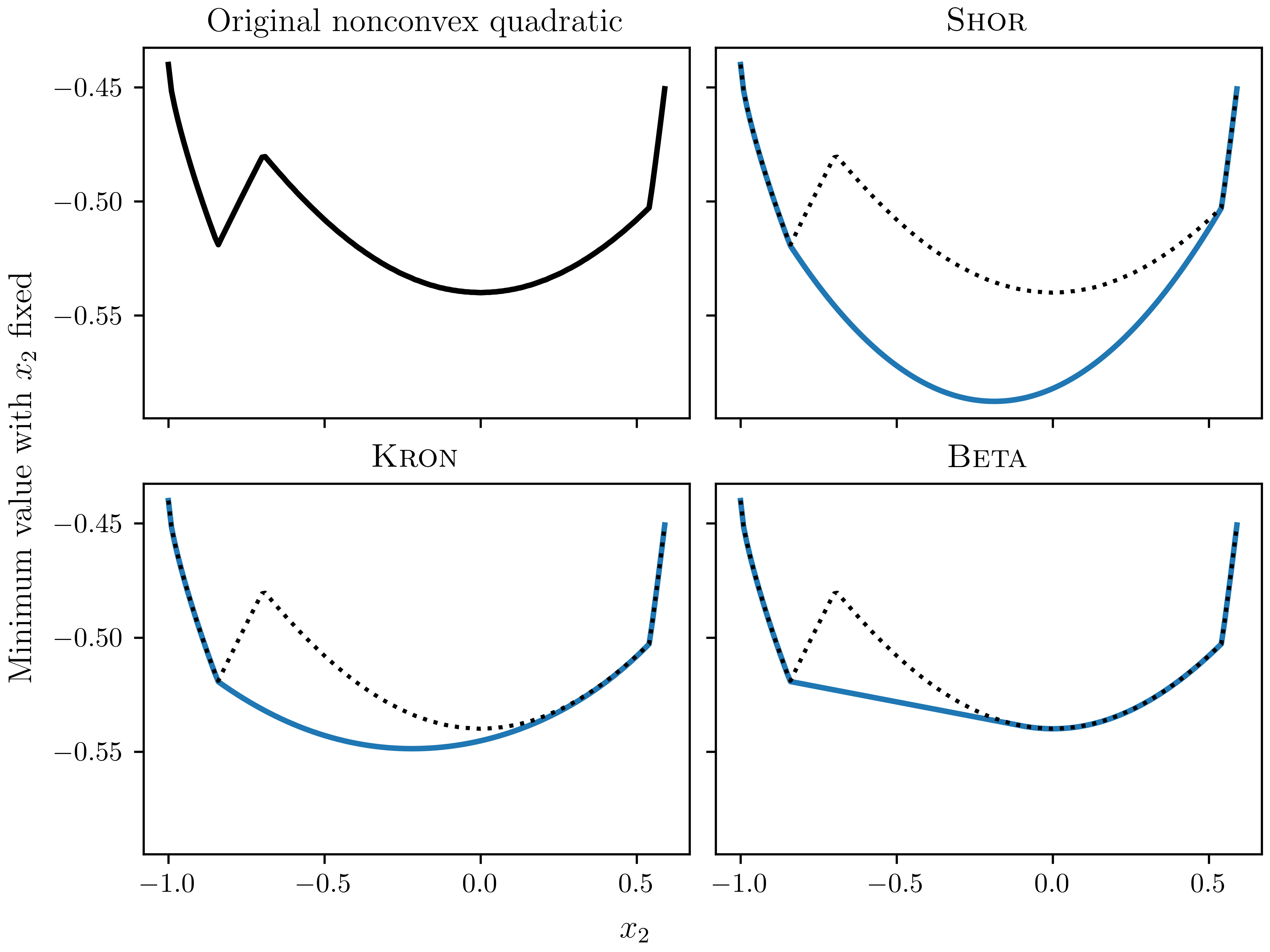
Figure 1: Illustrations of Example 1

3.3 The exact case $m=2$

For $m=2$, the auxiliary variable $\beta$ is inserted between $x^{T}x$ and both linear functions $\rho_{i}^{2}-c_{i}^{T}c_{i}+2c_{i}^{T}x$ for $i=1,2$. When $x^{T}x$ is strictly less than both linear functions, there are multiple values of $\beta$, which are feasible for the same value of $x$. To remove this ambiguity, we can actually force $\beta=\min_{i=1,2}\{\rho_{i}^{2}-c_{i}^{T}c_{i}+2c_{i}^{T}x\}$ by adding the quadratic complementarity equation

$$(\rho_{1}^{2}-c_{1}^{T}c_{1}+2c_{1}^{T}x-\beta)(\rho_{2}^{2}-c_{2}^{T}c_{2}+2c_{2}^{T}x-\beta)=(\ell_{1}^{T}w)(\ell_{2}^{T}w)=0$$

to the definition of $\mathcal{K}$. Formally, we define

$$\mathcal{K}^{0} :=\left\{w\in\mathcal{K}:(\ell_{1}^{T}w)(\ell_{2}^{T}w)=0\right\},$$

$$\mathcal{H}^{0} :=\operatorname{conic.hull}\{W=ww^{T}:w\in\mathcal{K}^{0}\},$$

$$\mathcal{R}^{0} :=\{W\in\mathcal{R}:\ell_{1}^{T}W\ell_{2}=0\}.$$

Note that optimizing $x^{T}Qx+2q^{T}x$ over $\mathcal{K}^{0}\cap\{{\color[rgb]{0,0,0}w}:\alpha=1\}$ is equivalent to (QP) because $\beta$ is artificial. We have the following exactness theorem, whose proof is delayed until Section 5:

Theorem 1.

Regarding the ball-constrained set (4), for $m=2$, it holds that $\mathcal{H}^{0}=\mathcal{R}^{0}$.

This ensures that, for $m=2$, (QP) is equivalent to

$$\min\left\{\widehat{Q}\bullet W:W\in\mathcal{R},\ W_{11}=1,\ \ell_{1}^{T}W\ell_{2}=0\right\}=\min\left\{\widehat{Q}\bullet W:W\in\mathcal{R}^{0},\ W_{11}=1\right\},$$

that is, equivalent to Beta with the strengthened constraint $\ell_{1}^{T}W\ell_{2}=0$.

To verify Theorem 1 empirically, we generated 1,000 feasible instances of (QP) for each of the dimension pairs $(n,m)\in\{(2,2),(4,2),({\color[rgb]{0,0,0}6},2)\}$ following the method of [9]; see section 5.3 of that paper and the discussion therein. The idea is to first generate and optimize globally an instance of (QP) with $m=1$ and then to add a second ball constraint, which cuts off the optimal solution just calculated. The resulting problem is likely to possess multiple good candidates for optimal solutions, thus ostensibly making it a more challenging instance of (QP). We call these the Martinez instances following the terminology in [9].

Among the total 3,000 instances generated, we specifically excluded ones that were already solved by Shor. This was done in order to eliminate the “easiest” instances, i.e., the ones that can already be handled by the simplest relaxation. In fact, for random instances such as the ones described, the percentage of instances already solved by Shor increases empirically as $n$ grows. Hence, limiting the experiments to the (relatively small) subset of instances that are not solved by Shor allows a more focused comparison of the performance of Kron and Beta.

$n$	$m$	# Instances	# Solved		Total Time (s)
			Kron	Beta	Shor	Kron	Beta
2	2	1,000	955	1,000	0.4	2.0	0.8
4	2	1,000	884	1,000	0.7	13.5	1.0
6	2	1,000	882	1,000	0.9	181.4	1.6

Table 1: Number of instances of (QP) solved by Kron and Beta over 3,000 randomly generated Martinez instances, which were not already solved by Shor. Instances are grouped by dimensions $(n,m)$. Also shown are the total time (in seconds) to optimize all instances for each method in each grouping. Times for Shor are also shown for reference.

Table 1 shows the results of our experiments. We see that, while Kron solves many instances, Beta solves all instances, as ensured by Theorem 1, in much less time. In fact, Beta takes just a bit more time than Shor.

Eltved and Burer [17] also optimized instances of (QP) with $m=2$, and they reported that their method, which is at least as strong as Kron, was unable to solve 267 randomly generated instances with $n$ ranging from 2 to 10; see table 6 therein. We ran Beta on these instances and globally solved all of them.

3.4 The general case $m\geq 3$

We now investigate the use of Kron and Beta to approximate instances of (QP) with $m\geq 3$. To this end, we generated random instances of the following problem, which we call max-norm and which has recently been studied in [16]:

In $\mathbb{R}^{n}$, given a point $p$ and $m$ balls containing the origin, find a point in the intersection of the balls with maximum distance to $p$.

This is an instance of (QP) with $Q=-I$ and $q=p$. We have chosen this class because it seems to be an interesting geometric problem, which is also NP-hard [16].

Specifically, the first ball is taken to be the unit ball, and the remaining $m-1$ balls are generated with random centers $c_{i}$ in the unit ball. Then the random radii $\rho_{i}$ for $i=2,\ldots,m$ are generated each in $\|c_{i}\|+U(0,1.5)$, where $U(0,1.5)$ is continuous uniform between 0 and 1.5. In particular, this guarantees that $x=0$ is in the resulting feasible set. Finally, $p$ is generated uniformly in the ball of radius 4 centered at the origin, and as such could be either inside or outside the feasible set. As in the previous subsection, we exclude instances that are solved by Shor in order to remove the easiest instances and focus on the performance of Beta relative to Kron.

We also examined the so-called gap closure for each relaxation. For a given instance, let $s^{*}$ be the optimal value of Shor, and let $v$ be the best (i.e., minimum) feasible value from the solutions embedded within the three relaxations Shor, Kron, and Beta at optimality. Then

gap closure for Kron $$:=\left(\frac{\text{[optimal value for \text{\sc Kron}]}-s^{*}}{v-s^{*}}\right)\times 100\%$$

gap closure for Beta $$:=\left(\frac{\text{[optimal value for \text{\sc Beta}]}-s^{*}}{v-s^{*}}\right)\times 100\%$$

A gap closure of 0% means that the relaxation did not improve upon Shor, and a gap closure of 100% means that the relaxation was exact.

Tables 2 and 3 show the results of Kron and Beta on 1,000 max-norm instances for three pairs of dimensions $(n,m)$. These results show clearly that Beta significantly outperforms Kron in terms of both number of instances solved and the average gap closed. In terms of timings, we see that Beta requires significantly less time. Furthermore, no instances were solved by Kron and simultaneously unsolved by Beta. This suggests empirically that Beta is always at least as strong as Kron, although we do not have a formal proof establishing this.

$n$	$m$	# Instances	# Solved		Total Time (s)
			Kron	Beta	Shor	Kron	Beta
2	5	1,000	208	977	0.3	14.7	1.1
2	9	1,000	412	973	0.4	153.1	1.9
4	9	1,000	2	908	0.8	2435.6	3.9

Table 2: Number of max-norm instances solved by Kron and Beta on 3,000 instances unsolved by Shor. Instances are grouped by dimensions $(n,m)$. Also included are the total time (in seconds) to optimize all instances for each method in each grouping.

Solution Status		# Instances	Avg Gap Closed
Kron	Beta		Kron	Beta
unsolved	unsolved	142	6%	29%
unsolved	solved	2236	30%	100%
solved	unsolved	0	-	-
solved	solved	622	100%	100%

Table 3: Average gap closures for Table 2. Instances are grouped by solution status for Kron and Beta.

As a final experiment, to judge the time required to optimize Beta as a function of $n$ and $m$, we computed the mean time to optimize a single random instance for 36 different combinations of $(n,m)$ ranging from $(2,2)$ to $(64,64)$. For each mean calculation, the sample size was 100. From Table 4, we see that our relaxation can be optimized in tens of seconds for modest values of $n$ and $m$.

	$m$
$n$	2	4	8	16	32	64
2	0.0	0.0	0.0	0.0	0.0	0.5
4	0.0	0.0	0.0	0.0	0.1	1.0
8	0.0	0.0	0.0	0.0	0.2	2.4
16	0.0	0.0	0.0	0.1	0.5	4.2
32	0.0	0.0	0.1	0.3	1.3	8.3
64	0.1	0.2	0.4	1.0	3.9	40.6

Table 4: Average time (in seconds) to optimize the Beta relaxation of 100 random max-norm instances for various combinations of $(n,m)$.

4 Extensions

In this section, we provide two extensions, which use the $\beta$ idea described in Section 3.

4.1 Linear upper bounds on the norm

Consider nonconvex quadratic programming over the set

$$\left\{x\in\mathbb{R}^{n}:\begin{array}[]{l}\|x\|\leq 1\\ \|x\|\leq g+h^{T}x\end{array}\right\},$$ (5)

where $g$ is a scalar and $h$ is a vector. We assume (5) is nonempty, but otherwise no particular assumptions are made on $g$ and $h$. Kelly et al. [19] studied this case using a disjunctive SDP approach; see also the discussion in Section 2.2.

As before, we introduce the auxiliary variable $\beta\in\mathbb{R}$ into (5), homogenize, enforce complementarity, and consider the cone

$$\mathcal{K}^{0}=\left\{w\in\mathbb{R}^{n+2}:P^{T}w\in\mathcal{SOC}^{n+1},\ \ell_{i}^{T}w\geq 0\ \forall\ i=1,2,\ (\ell_{1}^{T}w)(\ell_{2}^{T}w)=0\right\},$$

where

$$P:=\begin{pmatrix}0&0\\ 0&I_{n}\\ 1&0\end{pmatrix}\in\mathbb{R}^{(n+2)\times(n+1)},\quad\ell_{1}:=\begin{pmatrix}1\\ 0\\ -1\end{pmatrix}\in\mathbb{R}^{n+2},\quad\ell_{2}:=\begin{pmatrix}g\\ h\\ -1\end{pmatrix}\in\mathbb{R}^{n+2}.$$

Then Section 2 provides the following relaxation of $\mathcal{H}^{0}:=\operatorname{conic.hull}\{ww^{T}\in\mathbb{S}^{n+1}:w\in\mathcal{K}^{0}\}$:

$$\mathcal{R}^{0} :=\left\{W\in\mathcal{PSD}^{n+2}:\begin{array}[]{l}J_{n+1}\bullet P^{T}WP\geq 0\\ \ell_{1}^{T}W\ell_{2}=0\\ P^{T}W\ell_{i}\in\mathcal{SOC}^{n+1}\ \ \forall\ i=1,2\end{array}\right\}.$$

As with Theorem 1, we can prove that $\mathcal{R}^{0}$ captures the convex hull exactly.

Theorem 2.

Regarding the feasible set (5), it holds that $\mathcal{H}^{0}=\mathcal{R}^{0}$.

Proof.

The same proof for Theorem 1 handles this case as well. ∎

4.2 Two Trust Region Subproblem

As another extension, we consider the problem of minimizing a nonconvex quadratic over the intersection of two full-dimensional ellipsoids, i.e., the TTRS mentioned in the Introduction:

$$\min_{x\in\mathbb{R}^{n}}\left\{x^{T}Qx+2\,q^{T}x:\begin{array}[]{l}\|H_{i}x-c_{i}\|\leq\rho_{i}\quad\forall\ i=1,2\end{array}\right\},$$ (6)

where $H_{i}$ are full-rank matrices and $c_{i},\rho_{i}$ are as in (QP). By a change of variables, we may assume without loss of generality that $H_{1}=I_{n}$, $c_{1}=0$, and $\rho_{1}=1$, i.e., that the first ellipsoid is the unit ball. As with the ball case, the relaxation $\text{\sc Shor}\cap\text{\sc Kron}$ is applicable; see, in particular, the study by Anstreicher [2].

By another change of variables, we can further assume that $H_{2}$ is diagonal without loss of generality, in which case the feasible set can be rewritten as

$$\left\{x\ :\ x^{T}x\leq 1,\ \ \sum_{j=1}^{n}[H_{2}]_{j}^{2}x_{j}^{2}\leq\rho_{2}^{2}-c_{2}^{T}c_{2}+2c_{2}^{T}H_{2}x.\right\}$$

We next introduce $n$ new artificial variables $\beta_{j}$ satisfying $x_{j}^{2}\leq\beta_{j}$ and then homogenize and enforce complementarity:

$$\mathcal{K}:=\left\{w=\begin{pmatrix}\alpha\\ x\\ \beta\end{pmatrix}\in\mathbb{R}^{2n+1}\ :\ \begin{array}[]{l}P_{j}^{T}w\in\mathcal{SOC}^{3}\quad\forall\ j=1,\ldots,n\\ \ \ell_{i}^{T}w\geq 0\quad\forall\ i=1,2\\ (\ell_{1}^{T}w)(\ell_{2}^{T}w)=0\end{array}\right\},$$

where $e_{j}\in\mathbb{R}^{n}$ is the $j$-th standard unit vector,

$$P_{j}:=\begin{pmatrix}1/2&0&0\\ 0&0&e_{j}\\ 0&e_{j}&0\end{pmatrix}T_{3}\in\mathbb{R}^{(2n+1)\times 3}\ \ \forall\ j=1,\ldots,n,$$

and

$$\ell_{i}:=\begin{pmatrix}\rho_{i}^{2}-c_{i}^{T}c_{i}\\ 2H_{i}c_{i}\\ -\operatorname{diag}(H_{i}^{2})\end{pmatrix}\in\mathbb{R}^{2n+1}\ \ \forall\ i=1,2.$$

Note that, this formulation has $2n+1$ variables, $n$ SOC constraints of size 3, two linear constraints, and one complementarity constraint. Following the development in Section 2, our relaxation is then

$$\mathcal{R}^{0} :=\left\{W\in\mathcal{PSD}^{2n+1}:\begin{array}[]{l}J_{3}\bullet P_{j}^{T}WP_{j}\geq 0\ \ \forall\ j=1,\ldots,n\\ \ell_{1}^{T}W\ell_{2}=0\\ P_{j}^{T}W\ell_{i}\in\mathcal{SOC}^{3}\ \ \forall\ i=1,2,\ j=1,\ldots,n\\ (\operatorname{Arr}_{3}\boxtimes\operatorname{Arr}_{3})(P_{k}^{T}WP_{j})\in\mathcal{PSD}^{9}\ \ \forall\ 1\leq j<k\leq n\end{array}\right\}.$$

The paper [9] studied a relaxation of (6), which was based on rewriting the unit ball as the intersection of a semi-infinite number of half-spaces:

$$\left\{x:\begin{array}[]{l}\|x\|\leq 1\\ \|H_{2}-c_{2}\|\leq\rho_{2}\end{array}\right\}=\left\{x:\begin{array}[]{l}u^{T}x\leq 1\ \forall\ \|u\|=1\\ \|H_{2}-c_{2}\|\leq\rho_{2}\end{array}\right\}.$$

In doing so, the authors constructed a relaxation, which was a semi-infinite analog of $\text{\sc Shor}\cap\text{\sc RLT}\cap\text{\sc SOCRLT}$—as introduced in Section 2—which could nevertheless be optimized in polynomial-time in this special case. As a byproduct of this research, the authors introduced a collection of 212 instances of (6) with sizes $n\in\{5,10,20\}$, which were not solved by $\text{\sc Shor}\cap\text{\sc RLT}\cap\text{\sc SOCRLT}$.

These 212 instances have been revisited by Anstreicher [2], who showed that $\text{\sc Shor}\cap\text{\sc Kron}$ solves 77. Another approach by Yang and Burer [11] solves 29 instances. Finally, a recent cut-generation approach by Consolini and Locatelli [15] solves 211, i.e., all but one of the 212 instances. We applied our relaxation $\mathcal{R}^{0}$ to the same instances and solved all 212. The largest instances (size $n=20$) were solved in 0.374 seconds on average.

5 Proof of Theorem 1

In this section, we prove Theorem 1 from Section 3, which states that

$$\mathcal{H}^{0}:=\operatorname{conic.hull}\left\{ww^{T}\in\mathbb{S}^{n+2}:\begin{array}[]{l}P^{T}w\in\mathcal{SOC}^{n+2}\\ \ell_{i}^{T}w\geq 0\ \ \forall\ i=1,2\\ (\ell_{1}^{T}w)(\ell_{2}^{T}w)=0\end{array}\right\}$$

equals

$$\mathcal{R}^{0}:=\left\{W\in\mathcal{PSD}^{n+2}:\begin{array}[]{l}J_{n+2}\bullet P^{T}WP\geq 0\\ P^{T}W\ell_{i}\in\mathcal{SOC}^{n+2}\ \ \forall\ i=1,2\\ \ell_{1}^{T}W\ell_{2}=0\end{array}\right\}.$$

A closely related result is Theorem 2.7 in [27], but our proof follows a technique from [8].

We first prove some lemmas. To simplify notation, let $J:=J_{n+2}$ and $\mathcal{SOC}:=\mathcal{SOC}^{n+2}$ throughout the rest of this section. Our first lemma states some straightforward properties of $J$.

Lemma 1.

Regarding $J$, it holds that:

1. If $v\in\mathcal{SOC}$, then $Jv\in\mathcal{SOC}$, and hence $w^{T}Jv\geq 0$ for all $w\in\mathcal{SOC}$.

2. If $v\in\operatorname{bd}(\mathcal{SOC})$, then $v^{T}Jv=0$.

The next two lemmas are analogous to the exactness results of Shor and $\text{\sc Shor}\cap\text{\sc SOCRLT}$ discussed in Section 2.2.

Lemma 2.

$\operatorname{conic.hull}\{ww^{T}:P^{T}w\in\mathcal{SOC}\}=\{W\in\mathcal{PSD}^{n+2}:J\bullet P^{T}WP\geq 0\}.$

Proof.

This can be proven, for example, by showing that all extreme rays of the right-hand-side set have rank-1, which can in turn be shown via Pataki’s bound on the rank of extreme matrices of SDP-representable sets [21]. ∎

Lemma 3.

Fix $i=1$ or $i=2$. It holds that

$$\operatorname{conic.hull}\left\{ww^{T}:\begin{array}[]{l}P^{T}w\in\mathcal{SOC}\\ \ell_{i}^{T}w\geq 0\end{array}\right\}=\left\{W\in\mathcal{PSD}^{n+2}:\begin{array}[]{l}J\bullet P^{T}WP\geq 0\\ P^{T}W\ell_{i}\in\mathcal{SOC}\end{array}\right\}.$$

Proof.

In the statement of the proposition, let $\mathcal{H}[i]$ be the left-hand-side set, and let $\mathcal{R}[i]$ be the right-hand side. Clearly $\mathcal{H}[i]\subseteq\mathcal{R}[i]$. We show the reverse inclusion by proving $\mathcal{R}[i]$ has rank-1 extreme rays. Indeed, let $W\neq 0$ be an arbitrary extreme ray in $\mathcal{R}[i]$. We will show $\operatorname{rank}(W)=1$ by considering three cases .

First consider when $P^{T}W\ell_{i}\in\operatorname{int}(\mathcal{SOC})$, in which case $W$ must also be extreme in $\{W\in\mathcal{PSD}^{n+2}:J\bullet P^{T}WP\geq 0\}$. Then $\operatorname{rank}(W)=1$ by Lemma 2.

Next consider when $P^{T}W\ell_{i}\in\operatorname{bd}(\mathcal{SOC})$ with $W\ell_{i}=0$. Using Lemma 2, we write $W=\sum_{k}w^{k}(w^{k})^{T}$ for $w^{k}$ satisfying $P^{T}w^{k}\in\mathcal{SOC}$. We then have

$$W\ell_{i}=0\quad\Rightarrow\quad\ell_{i}^{T}W\ell_{i}=0\quad\Rightarrow\quad\sum_{k}(\ell_{i}^{T}w^{k})^{2}=0\quad\Rightarrow\quad\ell_{i}^{T}w^{k}=0\ \ \forall\ k,$$

which proves $W\in\mathcal{H}[i]$ and hence $W$ is extreme in $\mathcal{H}[i]$. Thus, $\operatorname{rank}(W)=1$, as desired.

Finally, consider when $P^{T}W\ell_{i}\in\operatorname{bd}(\mathcal{SOC})$ with $W\ell_{i}\neq 0$. Define $v:=W\ell_{i}\neq 0$ so that $P^{T}v\in\operatorname{bd}(\mathcal{SOC})$. In addition, $W\in\mathcal{PSD}^{n+2}$ implies $\ell_{i}^{T}v=\ell_{i}^{T}W\ell_{i}\geq 0$. Hence, we conclude that $vv^{T}$ is a nonzero member of $\mathcal{H}[i]\subseteq\mathcal{R}[i]$. Next, for small $\epsilon>0$, define $W_{\epsilon}:=W-\epsilon\,vv^{T}$; we claim $W_{\epsilon}\in\mathcal{R}[i]$. Indeed, $W_{\epsilon}\in\mathcal{PSD}^{n+2}$ because it is a rank-1 perturbation of $W\in\mathcal{PSD}^{n+2}$ with $v\in\operatorname{Range}(W)$ [10, Lemma 2]. Moreover, $P^{T}v\in\operatorname{bd}(\mathcal{SOC})$ implies by Lemma 1(ii) that

$$J\bullet P^{T}W_{\epsilon}P=J\bullet P^{T}WP-\epsilon(P^{T}v)^{T}J(P^{T}v)=J\bullet P^{T}WP-\epsilon\cdot 0\geq 0.$$

We also have

$$P^{T}W_{\epsilon}\ell_{i}=P^{T}W\ell_{i}-\epsilon(\ell_{i}^{T}v)P^{T}v=(1-\epsilon\cdot\ell_{i}^{T}v)P^{T}v\in\operatorname{bd}(\mathcal{SOC}).$$

Thus, when $\epsilon>0$ is small, $W_{\epsilon}\in\mathcal{R}[i]$ as claimed. Then the equation $W=W_{\epsilon}+\epsilon\,vv^{T}$ and the fact that $W$ is extreme in $\mathcal{R}[i]$ imply $W$ must be a positive multiple of $vv^{T}$, i.e., $\operatorname{rank}(W)=1$, as desired. ∎

Our next lemma is a technical result about extreme rays in the intersection of two closed convex cones.

Lemma 4.

Let $\mathcal{P}$ be a closed convex cone, and let $\mathcal{Q}$ be a half-space containing the origin. Every extreme ray of $\mathcal{P}\cap\mathcal{Q}$ is either an extreme ray of $\mathcal{P}$ or can be expressed as the sum of two extreme rays of $\mathcal{P}$.

Proof.

See [8, Lemma 5]. ∎

We are now ready to prove Theorem 1.

Proof.

Since $\mathcal{H}^{0}\subseteq\mathcal{R}^{0}$ by construction, we show the reverse inclusion by proving that every extreme ray $W$ of $\mathcal{R}^{0}$ has rank 1 and hence is an element of $\mathcal{H}^{0}$. We define $v_{i}:=W\ell_{i}$ for $i=1,2$. Note that $v_{1}v_{1}^{T}\in\mathcal{H}^{0}$ because $\ell_{1}^{T}v_{1}=\ell_{1}^{T}W\ell_{1}\geq 0$, $\ell_{2}^{T}v_{1}=\ell_{2}^{T}W\ell_{1}=0$, and $P^{T}v_{1}=P^{T}W\ell_{1}\in\mathcal{SOC}$. A similar argument shows $v_{2}v_{2}^{T}\in\mathcal{H}^{0}$.

We first consider the case when $v_{1}=0$. Applying Lemma 3 for the case $i=2$, we express $W$ as

$$W=\sum_{k}w^{k}(w^{k})^{T},\quad P^{T}w^{k}\in\mathcal{SOC}\text{ and }\ell_{2}^{T}w^{k}\geq 0\quad\forall\ k.$$

As in the proof of Lemma 3, $v_{1}=0$ then implies $\ell_{1}^{T}w^{k}=0$ for all $k$. So $W\in\mathcal{H}^{0}$, and because $W$ is extreme in $\mathcal{R}^{0}\supseteq\mathcal{H}^{0}$, it must have rank 1. A similar argument shows $\operatorname{rank}(W)=1$ for the case $v_{2}=0$.

So we assume from this point forward that $v_{i}:=W\ell_{i}\neq 0$ for both $i=1,2$. Since $W\in\mathcal{PSD}^{n+2}$ ensures $W\ell_{i}=0\Leftrightarrow\ell_{i}^{T}W\ell_{i}=0$, we have $\ell_{i}^{T}v_{i}=\ell_{i}^{T}W\ell_{i}>0$ for both $i$.

The second case we consider assumes $J\bullet P^{T}WP=0$ and $P^{T}v_{i}=P^{T}W\ell_{i}\in\operatorname{int}(\mathcal{SOC})$ for both $i=1,2$. Then $W$ is extreme for the equality-constrained cone $\{W\in\mathcal{PSD}^{n+2}:J\bullet P^{T}WP=0,\ell_{1}^{T}W\ell_{2}=0\}$, which in turn implies that $W$ is extreme for the inequality-constrained cone $\mathcal{P}\cap\mathcal{Q}$, where

$$\mathcal{P}:=\left\{W\in\mathcal{PSD}^{n+2}:J\bullet P^{T}WP\geq 0\right\},\ \ \ \ \mathcal{Q}:=\{W\in\mathbb{S}^{n+2}:\ell_{1}^{T}W\ell_{2}\geq 0\},$$

Applying Lemma 2 with $\mathcal{P}$ and Lemma 4 with $\mathcal{P}\cap\mathcal{Q}$, we conclude that $\operatorname{rank}(W)\leq 2$. If its rank equals 1, we are done. So assume $\operatorname{rank}({\color[rgb]{0,0,0}W})=2$. We derive a contradiction to the assumption that $W$ is extreme in $\mathcal{R}^{0}$. Consider the equation

$$U:=\begin{pmatrix}\ell_{1}^{T}\\ \ell_{2}^{T}\\ I\end{pmatrix}W\begin{pmatrix}\ell_{1}&\ell_{2}&I\end{pmatrix}=\begin{pmatrix}\ell_{1}^{T}W\ell_{1}&\ell_{1}^{T}W\ell_{2}&\ell_{1}^{T}W\\ \ell_{2}^{T}W\ell_{1}&\ell_{2}W\ell_{2}&\ell_{2}^{T}W\\ W\ell_{1}&W\ell_{2}&W\end{pmatrix}=\begin{pmatrix}\ell_{1}^{T}v_{1}&0&v_{1}^{T}\\ 0&\ell_{2}^{T}v_{2}&v_{2}^{T}\\ v_{1}&v_{2}&W\end{pmatrix},$$

and recall that $\ell_{1}^{T}v_{1}>0$ and $\ell_{2}^{T}v_{2}>0$. It holds that $U$ is PSD with $\operatorname{rank}(U)\leq\operatorname{rank}(W)=2$, and hence the $\operatorname{Range}(W)$ is spanned by $\{v_{1},v_{2}\}$ because the first two columns of $U$ are clearly linearly independent. Then, because $W\succeq 0$ with $\operatorname{rank}(W)=2$, it must hold that

$$W=\lambda_{1}v_{1}v_{1}^{T}+\lambda_{2}v_{2}v_{2}^{T},$$

for some positive multipliers $\lambda_{i}>0$. However, this contradicts the assumption that $W$ is extreme in $\mathcal{R}^{0}$ due to the fact that both $v_{1}v_{1}^{T}$ and $v_{2}v_{2}^{T}$ are elements of $\mathcal{H}^{0}\subseteq\mathcal{R}^{0}$.

For our third and final case, we assume $J\bullet P^{T}WP>0$, $P^{T}v_{1}\in\operatorname{bd}(\mathcal{SOC})$, or $P^{T}v_{2}\in\operatorname{bd}(\mathcal{SOC})$. Let us consider two perturbations of $W$:

$$W_{\epsilon_{i}}:=W-\epsilon_{i}\,v_{i}v_{i}^{T}\quad\forall\ i=1,2$$

for two parameters $\epsilon_{i}>0$. We claim that $W_{\epsilon_{i}}\in\mathcal{R}^{0}$ for at least one $i$, in which case $W$ must be rank-1 as argued in the proof of Lemma 3.

Using $W\in\mathcal{R}^{0}$, we first argue that each $W_{\epsilon_{i}}$ satisfies all constraints of $\mathcal{R}^{0}$, except possibly $J\bullet P^{T}W_{\epsilon_{i}}P\geq 0$. Fix $i=1$; the proof for $i=2$ is similar. We know $W_{\epsilon_{1}}\in\mathcal{PSD}^{n+2}$ since $v_{1}\in\operatorname{Range}(W)$ [10, Lemma 2]. We also have

$$P^{T}W_{\epsilon_{1}}\ell_{1}=P^{T}v_{1}-\epsilon_{1}P^{T}v_{1}(v_{1}^{T}\ell_{1})=(1-\epsilon_{1}(v_{1}^{T}\ell_{1}))P^{T}v_{1}\in\mathcal{SOC}$$

for small $\epsilon_{1}>0$. Furthermore, noting that $v_{1}^{T}\ell_{2}=\ell_{1}^{T}W\ell_{2}=0$, we see

$$P^{T}W_{\epsilon_{1}}\ell_{2}=P^{T}v_{2}-\epsilon_{1}P^{T}v_{1}(\ell_{1}^{T}W\ell_{2})=P^{T}v_{2}-\epsilon_{1}P^{T}v_{1}\cdot 0=P^{T}v_{2}\in\mathcal{SOC}.$$

Finally,

$$\ell_{1}^{T}W_{\epsilon_{1}}\ell_{2}=\ell_{1}^{T}W\ell_{2}-\epsilon_{1}(\ell_{1}^{T}v_{1})(v_{1}^{T}\ell_{2})=\ell_{1}^{T}W\ell_{2}-\epsilon_{1}(\ell_{1}^{T}v_{1})(\ell_{1}^{T}W\ell_{2})=0-\epsilon_{1}\cdot\ell_{1}^{T}v_{1}\cdot 0=0,$$

as desired.

We now claim that at least one $W_{\epsilon_{i}}$ satisfies the remaining constraint

$$J\bullet P^{T}W_{\epsilon_{i}}P=J\bullet P^{T}WP-\epsilon_{i}J\bullet(P^{T}v_{i})(P^{T}v_{i})^{T}\geq 0$$

for small $\epsilon_{i}>0$, thus completing the proof as discussed above. If $J\bullet P^{T}WP>0$, then both $W_{\epsilon_{i}}$ satisfy the inequality. If $P^{T}v_{1}\in\operatorname{bd}(\mathcal{SOC})$, then $W_{\epsilon_{1}}$ satisfies the inequality because $J\bullet(P^{T}v_{i})(P^{T}v_{i})^{T}=0$ by Lemma 1(ii). Similarly if $P^{T}v_{2}\in\operatorname{bd}(\mathcal{SOC})$, then $W_{\epsilon_{2}}$ satisfies the inequality. ∎

6 Conclusions

In this paper, we have constructed strong relaxations for (QP) by transforming its feasible set, lifting to one higher dimension, and employing standard relaxation techniques from the literature. Our computational results demonstrate the strength of our relaxation, and the time required for solving our relaxation is small compared to those in the literature. We have also shown that our relaxation is exact for the case of two balls.

There are many open questions related to this research. For example, is it possible to prove that our relaxation Beta is always at least as tight as Kron, as supported by the computational evidence? Furthermore, is Beta provably as strong as the method of [17]? Is it possible to extend Theorem 1 to the case of more constraints? Finally, even when our relaxation is not exact in practice for $m\geq 3$, could it be used within an effective global optimization algorithm of (QP)?

Statements and Declarations

The author declares that he has no competing interests.

References

• [1] T. A. Almaadeed, S. Ansary Karbasy, M. Salahi, and A. Hamdi. On indefinite quadratic optimization over the intersection of balls and linear constraints. J. Optim. Theory Appl., 194(1):246–264, 2022.
• [2] K. M. Anstreicher. Kronecker product constraints with an application to the two-trust-region subproblem. SIAM Journal on Optimization, 27(1):368–378, 2017.
• [3] M. ApS. The MOSEK Fusion API for Python Manual. Version 10.0.37., 2023.
• [4] G. Azuma, M. Fukuda, S. Kim, and M. Yamashita. Exact SDP relaxations for quadratic programs with bipartite graph structures. J. Global Optim., 86(3):671–691, 2023.
• [5] A. Beck and D. Pan. A branch and bound algorithm for nonconvex quadratic optimization with ball and linear constraints. J. Global Optim., 69(2):309–342, 2017.
• [6] D. Bienstock. A note on polynomial solvability of the CDT problem. SIAM Journal on Optimization, 26(1):488–498, 2016.
• [7] D. Bienstock and A. Michalka. Polynomial solvability of variants of the trust-region subproblem. In Proceedings of the Twenty-Fifth Annual ACM-SIAM Symposium on Discrete Algorithms, pages 380–390. ACM, New York, 2014.
• [8] S. Burer. A gentle, geometric introduction to copositive optimization. Math. Program., 151(1, Ser. B):89–116, 2015.
• [9] S. Burer and K. M. Anstreicher. Second-order-cone constraints for extended trust-region subproblems. SIAM Journal on Optimization, 23(1):432–451, 2013.
• [10] S. Burer, K. M. Anstreicher, and M. Dür. The difference between $5\times 5$ doubly nonnegative and completely positive matrices. Linear Algebra Appl., 431(9):1539–1552, 2009.
• [11] S. Burer and B. Yang. The trust region subproblem with non-intersecting linear constraints. Math. Program., 149(1-2, Ser. A):253–264, 2015.
• [12] S. Burer and Y. Ye. Exact semidefinite formulations for a class of (random and non-random) nonconvex quadratic programs. Math. Program., 181(1, Ser. A):1–17, 2020.
• [13] S. Burer and Y. Ye. Correction to: Exact semidefinite formulations for a class of (random and non-random) nonconvex quadratic programs. Math. Program., 190(1-2, Ser. A):845–848, 2021.
• [14] C. Chen, A. Atamtürk, and S. S. Oren. A spatial branch-and-cut method for nonconvex QCQP with bounded complex variables. Math. Program., 165(2, Ser. A):549–577, 2017.
• [15] L. Consolini and M. Locatelli. Sharp and fast bounds for the Celis-Dennis-Tapia problem. SIAM J. Optim., 33(2):868–898, 2023.
• [16] M. Costandin. On maximizing the distance to a given point over an intersection of balls ii, 2023.
• [17] A. Eltved and S. Burer. Strengthened SDP relaxation for an extended trust region subproblem with an application to optimal power flow. Math. Program., 197(1, Ser. A):281–306, 2023.
• [18] R. Jiang and D. Li. Second order cone constrained convex relaxations for nonconvex quadratically constrained quadratic programming. Journal of Global Optimization, 75(2):461–494, June 2019.
• [19] S. Kelly, Y. Ouyang, and B. Yang. A note on semidefinite representable reformulations for two variants of the trust-region subproblem. Manuscript, School of Mathematical and Statistical Sciences, Clemson University, Clemson, South Carolina, USA, 2022.
• [20] M. Locatelli. KKT-based primal-dual exactness conditions for the Shor relaxation. J. Global Optim., 86(2):285–301, 2023.
• [21] G. Pataki. On the rank of extreme matrices in semidefinite programs and the multiplicity of optimal eigenvalues. Math. Oper. Res., 23:339–358, 1998.
• [22] F. Rendl and H. Wolkowicz. A semidefinite framework for trust region subproblems with applications to large scale minimization. Math. Programming, 77(2, Ser. B):273–299, 1997.
• [23] H. D. Sherali and W. P. Adams. A reformulation-linearization technique for solving discrete and continuous nonconvex problems, volume 31 of Nonconvex Optimization and its Applications. Kluwer Academic Publishers, Dordrecht, 1999.
• [24] S. Sojoudi and J. Lavaei. Exactness of semidefinite relaxations for nonlinear optimization problems with underlying graph structure. SIAM J. Optim., 24(4):1746–1778, 2014.
• [25] J. F. Sturm and S. Zhang. On cones of nonnegative quadratic functions. Math. Oper. Res., 28(2):246–267, 2003.
• [26] A. L. Wang and F. Kılınç-Karzan. On the tightness of SDP relaxations of QCQPs. Math. Program., 193(1, Ser. A):33–73, 2022.
• [27] Y. Ye and S. Zhang. New results on quadratic minimization. SIAM J. Optim., 14(1):245–267 (electronic), 2003.
• [28] J. Zhen, D. de Moor, and D. den Hertog. An extension of the reformulation-linearization technique to nonlinear optimization. Manuscript, ETH Zürich, , Zürich, Switzerland, 2022.