Perturbative solution of fermionic sign problem in lattice Quantum Monte Carlo

Abstract

We develop a strong-coupling perturbation scheme for a generic Hubbard model around a half-filled particle-hole-symmetric reference system, which is free from the fermionic sign problem. The approach is based on the lattice determinantal Quantum Monte Carlo (QMC) method in continuous and discrete time versions for large periodic clusters in a fermionic bath. Considering the first-order perturbation in the shift of the chemical potential and of the second-neighbour hopping gives an accurate electronic spectral function for a parameter range corresponding to the optimally doped cuprate system for temperature of the order of $T=0.1t$, the region hardly accessible for the straightforward lattice QMC calculations. We discuss the formation of the pseudogap and the nodal-antinodal dichotomy for a doped Hubbard system in a strong-coupling regime with the interaction parameter $U$ equal to the bandwidth and the optimal value of the next-nearest-neighbor hopping parameter $t^{\prime}$ for high-temperature superconducting cuprates.

INTRODUCTION

Search for numerically exact solution of the $t-t^{\prime}-U$ Hubbard model in thermodynamic limit at arbitrary interaction strength, long-range hoppings and doping $\delta$ or, equivalently, chemical potential $\mu$ at low temperature $T=1/\beta$ is tremendously difficult. Modern computational approaches, based on the lattice determinantal Quantum Monte Carlo (QMC) methods have seen incredible progress in the half-filled case without $t^{\prime}$ SimonsPRX , but face an unacceptable fermionic sign problem for a general case related to cuprate high-temperature superconductivity (HTSC) problem, which is the main factor restricting the accuracy of QMC calculations for interacting fermionssign1 ; sign2 ; Troyer_sign ; Scalettar_sign2022 . A very important and largely unresolved problem is related to the next-nearest-neighbor hopping $t^{\prime}$ in the Hubbard model and its role in the tendency towards superconductivityDeveraux_Tp ; Deveraux_Hubb_Tp ; White_Plaquette_Dw ; Zhang_noSC ; Harland16 ; Harland20 ; danilov2022 .

On the other hand, the new class of diagrammatic Monte Carlo schemeProkofev_sign_blessing is claimed to have a “sign blessing” property which helps to reduce the effects of high-order diagrams. The state-of-the-art diagrammatic Monte Carlo scheme in the connected determinant mode (C-DET)Rossi_PRL based on efficient Continuous Time Quantum Monte Carlo(CT-QMC) scheme in the weak coupling technique(CT-INT) Rubtsov_CTINT gives unprecedented accuracy for the doped Hubbard modelFedor_PG ; Fedor_strong . It becomes possible to study formation of the pseudogap already at the beginning of strong coupling case with $U/t=6$ Fedor_PG . Nevertheless, exponential convergence of the C-DET scheme for weak interactions Rossi_2017 ; Homotopic_QMC , turns to a divergence at large $U$ values due to poles in the complex $U$-planeFedor_strong . This means that calculations for interactions close to the bandwidth $U/t\approx 8$ and temperature $T/t\approx 0.1$ are still within a prohibited area in the phase diagramFedor_strong .

There is a recent interesting attempt to use dynamical variational QMC scheme for the doped Hubbard model Imada_VQMC2020 ; Tremblay_VQMC2022 which gives a very reasonable description of the spectral function. The existence of the pseudogap can be explained in the simple model of electron fractionalization and appearing of “dark” fermion which is supported by $2\times 2$ cluster Dynamical Mean Field Theory (C-DMFT) Civelli_CDMFT_HFermion2016 ; Harland16 . Moreover, the experimental RIXS spectrum Huang_PG2022 of doped cuprate materials can be interpreted in such a theoretical model of the pseudogap formation. The larger cluster in the C-DMFT scheme for the doped case has an unacceptable fermionic sign problem within the QMC scheme. Recently, the importance of vertex corrections for pseudogap physics was discussed in the parquet formalism for dual fermions  Krien_2022 .

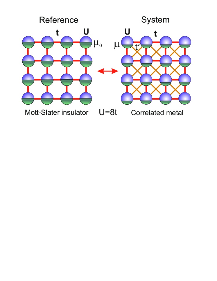
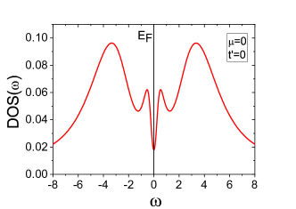
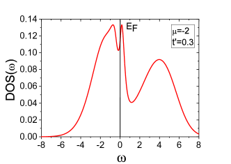
Figure 1: Schematic representation of a half-filled reference system for the doped square lattice. Bellow: calculated density of states (DOS) in presented scheme for $U=8$, Left: undoped case $\mu=0$ with $t^{\prime}=0$, Right: doped case $\mu=-2$ with $t^{\prime}/t=-0.3$

In this paper we discuss a different route to tackle the “sign problem” in the determinantal lattice QMC scheme and design a strong-coupling perturbative solution for a general Hubbard model. The starting point is related to the “reference system” idea Brener_refsys which is basically quite simple and straightforward. The conventional choice of the noninteracting Hamiltonian as the reference system for the perturbation AGD is justified by Wick’s theorem which allows to calculate exactly any many-particle Green’s functions: they are all expressed in terms of single-particle Green’s functions. The choice of single-site approximation like dynamical mean-field theory RevModPhys.68.13 as the reference system leads to the dual fermion technique RKL08 ; Brener_refsys . Actually, the reference system can be arbitrary assuming that we can calculate its Green’s functions of arbitrary order. Of course, in practice this is hardly doable.

At the same time, sometimes even taking into account the simplest, first-order diagram, seems to be quite successful. In the conventional weak-coupling expansion it is equivalent to the famous Hartree-Fock approximation Bethe which is able to catch a lot of important many-body physics including e.g. superconductivity within the BCS model. It can be shown IK1 ; IK2 ; IK3 that the unrestricted Hartree-Fock trial wave function is optimal within a very broad class of variational ground-state wave functions for different physical systems. It is worthwhile to mention here the very successful Peierls-Feynman-Bogoliubov variational principle Peierls_1938 ; Feynman_1972 ; Bogolyubov_1958 which can be formulated in the path-integral scheme. In this case, a good variational estimate of the system’s free energy $F$ with the Hamiltonian $H_{1}$ is achieved on an optimal reference system with the Hamiltonian $H_{0}$, namely $F_{1}\leq F_{0}+\langle H_{1}-H_{0}\rangle_{0}$. One can hope therefore that even first-order corrections to the properly chosen reference system will already give a rich and adequate enough physical picture. At least, this is definitely an assumption worth to be checked.

Here our reference system corresponds to the half-filled ($\mu=0$) particle-hole symmetric ($t^{\prime}=0$) case (Figure 1) where lattice Monte Carlo has no sign problem and the numerically exact solution for any practical value of $U$ is possible within a broad range of temperatures DQMC_Scalettar . Then we apply the lattice dual fermion perturbation theory RKL08 ; DF_Rev ; Brener_refsys to find the first-order perturbative corrections in $\mu$ and $t^{\prime}$. To this aim, it is sufficient to calculate the two-particle Green’s function, or, equivalently, four-leg vertex, which can be done accurately enough within the continuous time Quantum Monte Carlo. This approach can be considered as a far-going generalization of the Hartree-Fock approximation to the case of a dynamical effective interaction. Our reference system already has the main correlation effects in the lattice and shows characteristic “four-peak” structure with high-energy Hubbard bands around $\pm U/2$ and antiferromagnetic Slater bands close to the insulating gap (which can be seen in the density of states in Figure 1, left panel). After the dual fermion perturbation scheme the correlated metallic states with the DMFT-like ”three peak” structure appear with a pseudogap-like feature at a high temperature (the density of states in Figure 1, right panel). The results for the strong-coupling case ($U=W=8t$) with practically interesting values of the chemical potential and next-nearest-neighbour hoppings corresponding to cuprate superconductors have shown formation of a pseudogap and nodal-antinodal dichotomy (that is, well-defined quasiparticles in the nodal part of the Fermi surface and strong quasiparticle damping for the antinodal part) which makes this approximation a perspective for practical applications.

RESULTS

We have calculated the Green’s function for the doped two-dimensional Hubbard model for a periodic $8\times 8$ system with $U/t=8$, $t^{\prime}/t=-0.3$ and $\mu=-2.0$ in units of $t$ for $\beta=10$ (in units $1/t$) using a CT-INT version of the CT-QMC scheme Rubtsov_CTINT . Note that for the non-interacting Green’s function we used the infinite-lattice limit with periodic boundary conditions for the calculated $8\times 8$ system (see Section METHODS). This scheme reduces the cluster-size dependence for the bare Green’s function: in particular, the local one does not depend at all on the choice of the “simulation box”. On the other hand, it may underestimate the effect of $U$-interactions, since it appears only in the calculated cluster. This may explain a small gap in the half-filled reference system compare to a standard lattice determinantal QMC scheme Rost_QMC .

The results for the first-order dual-fermion perturbation from the half-filled system indicate the formation of correlated pseudogap electronic structure. Figure 2 shows the color map of the spectral function along the irreducible path ($\Gamma-X-M-\Gamma$) in the square Brillouin zone. For analytical continuation the newly developed scheme Gull_MaxEnt was used.

Several characteristic features of the correlated metallic phase in generic cuprate systems can be detected: formation of an extended pseudogap region around the $X$-point towards the $M$-point, a shadow antiferromagnetic band at energy $-2t$ near the $M$-point, a strongly renormalized metallic band near the nodal point around $\Gamma M/2$. Overall, the spectral function for $U=W$ clearly shows strong correlation features of the electronic structure far beyond a simple renormalized-band paradigm.

In order to see more clearly the pseudogap and nodal-antinodal dichotomy we plot the energy dependence of two spectral functions at the $X$- and $\Gamma M/2$-points in the Brillouin zone (Figure 3). While at the $X=(\pi,0)$-point there is a reasonably deep pseudogap fromation already at $\beta=10$, the nodal spectral function at $(\pi/2,\pi/2)$ has correlated metallic behaviour. A more unusual feature of the strong-coupling spectral function in Figure 2 is related with a ”shark mouth” pseudogap dip starting at $X$ in the direction to $M$ until the half way. One can see from the energy dependence of the spectral function in the direction of $X-M$ (Figure 4, middle panel) that the pseudogap splitting of the sharp quasiparticle peak at zero for the $XM/4$ point is even larger than at the $X$-point. The same feature was observed for a self-energy in the diagrammatic Monte Carlo (C-DET) investigation of the doped Hubbard model at $U/t=6$ Fedor_PG . We would like to point out that all these effects are not simply an artifact of the analytical continuation with the MaxEnt scheme and can be detected by inspection of the original complex Matsubara Green’s function from DF-QMC calculations (Figure 5). If we compare the $X=(\pi,0)$ and $XM/4=(\pi,\pi/4)$ points then both quasiparticle peaks located almost at the Fermi energy (the real part of $G({\mathbb{k}},\omega_{n})$ is close to zero, but the pseudogap or upturn of the imaginary part of $G({\mathbf{k}},\omega_{n})$ for the first Matsubara frequencies are more pronounced at the $(\pi,\pi/4)$-point. We have also checked this characteristic feature for the Hirsch-Fye QMC scheme Hirsch-Fye and different MaxEnt implementations. The general structure of this spectral function is similar to recent results of dynamical variational Monte Carlo schemes Imada_VQMC2020 ; Tremblay_VQMC2022 .

We plot a broadened Fermi surface using the momentum-dependent spectral function for the first Matsubara frequency (Figure 6). Comparison with the non-interacting tight-binding Fermi surface for the same doping shows a large region of the pseudogap around the $X$-point and formation of Fermi arcs near the nodal point. Moreover, one can understand that the pseudogap is more pronounced a bit away from the $X$-point towards the $M$-point, where the non-interacting Fermi surface crosses the Brillouin zone. We also compare the Fermi surface plot for smaller values of $U/t=5.6$, which was investigated in the diagrammatic Monte Carlo technique Wei_point ; Rossi_2020 ; this value is related to a plaquette degenerate point danilov2022 . While the Fermi surface for small $U/t=5.6$ agrees well with the results of the diagrammatic Monte Carlo approach Rossi_2020 and resembles the tight-binding one with only large broadening around the $X$-point, the $U/t=8$ results show already a formation of the pseudogap and Fermi arcs, that is, a nodal-antinodal dichotomy.

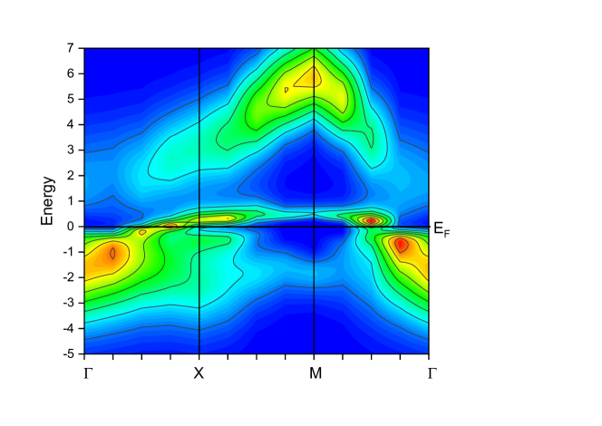
Figure 2: Spectral function $-1/\pi\Im G({\mathbb{k}},\omega)$ for dual fermion QMC (CT-INT) for $(8\times 8)$ lattice with $U=8$, $t^{\prime}/t=-0.3$, $\mu=-2.0$, and $\beta=10$.

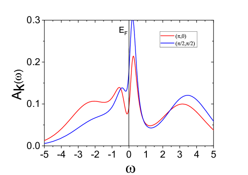
Figure 3: Spectral function $-1/\pi\Im G({\mathbb{k}},\omega)$ for two different k-points corresponds to anti-nodal and nodal k-points dual fermion QMC (CT-INT) for $(8\times 8)$ lattice with $U/t=8$ $t^{\prime}/t=-0.3$, $\mu=-2.0$ and $\beta=10$ .

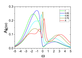
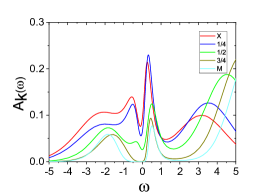
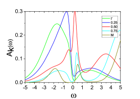
Figure 4: Spectral function $-1/\pi\Im G({\mathbb{k}},\omega)$ for three different k-directions in the Brillouin Zone, (left) $\Gamma-X$, (middle) $X-M$ and (right) ($\Gamma-M$) dual fermion QMC (CT-INT) for $(8\times 8)$ lattice with $U/t=8$ $t^{\prime}/t=-0.3$, $\mu=-2.0$ and $\beta=10$ .

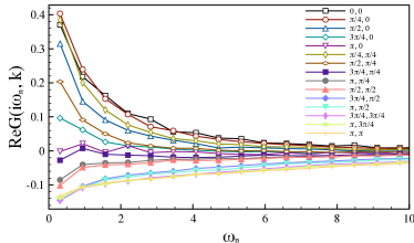
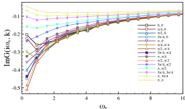
Figure 5: Green’s function $G({\mathbb{k}},\omega_{n})$ on the Matsubara axes for all 16 non-equivalent k-points in the Brillouin Zone for $8\times 8$ system, (left) Real part and (right) imaginary part for dual fermion QMC (CT-INT) with $U/t=8$ $t^{\prime}/t=-0.3$, $\mu=-2.0$ and $\beta=10$ .

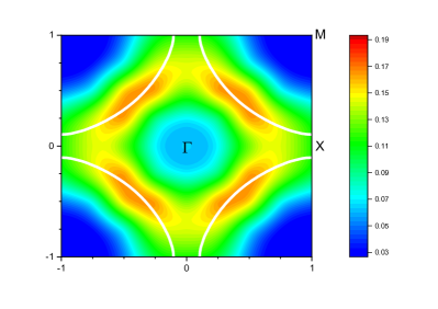
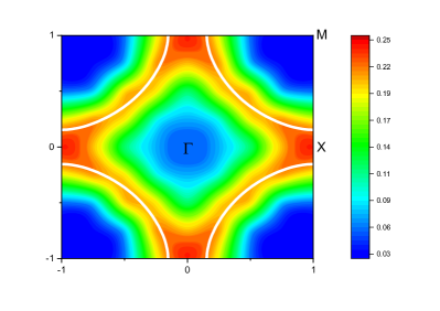
Figure 6: Spectral function of the square-lattice Hubbard model as a function of momentum at the first Matsubara frequency $G({\mathbb{k}},\omega_{0})$ for dual fermion QMC with $t^{\prime}/t=-0.3$, $\beta=10$ and $U/t=8$, $\mu=-2.0$ (left) $U/t=5.6$, $\mu=-0.9$ (right) . The non-interacting Fermi surface with the same doping is shown for comparisson as a white contour.

DISCUSSION

We developed, for Hubbard-like correlated lattice models, the first-order strong-coupling dual fermion expansion in the shift of the chemical potential (doping) and in the second-neighbour hoppings ($t^{\prime}$). The starting reference point corresponds to the half-filled particle-hole symmetric system which can be calculated numerically exactly, without the fermionic sign problem. For physically interesting parameter range of cuprate-like systems (around 10$\%$ doping and $t^{\prime}/t=-0.3$0 we can obtain a reasonable Green’s function for a periodic $8\times 8$ lattice for the temperature $T=0.1t$ . The formation of the pseudogap around the antinodal $X$-point and the nodal-antinodal dichotomy are clearly seen in the present approach.

We would like to point out a few main reasons why such a “super-perturbation” scheme works: first of all, the reference system already contains the main correlation effects which result in the four-peak structure of the density of states for the half-filled lattice Monte-Carlo calculations Rost_QMC ; second, the first-order strong-coupling perturbation relies on the lattice four-point vertex $\gamma_{1234}$ (Eq. (7)) which is obtained numerically exactly and has all the information about the spin and charge susceptibilities of the lattice; and third, if the dual perturbation Green’s function $\tilde{G}^{0}_{12}$ (Eq. (6)) is relatively small, results will be reasonable. The complicated question of convergence for such a dual-fermion perturbation can be checked numerically by calculating the second-order contribution in $\tilde{\Sigma}_{12}$. For this term one needs to calculate in the lattice QMC a six-point vertex $\gamma^{(6)}$ which will be also a direction of future developments. In principle, one can also discuss an instability towards antiferromagnetism or d-wave superconductivity, introducing symmetry-breaking fields White_Plaquette_Dw , which we also plan to investigate.

It is worthwhile to mention that for the starting reference system we can choose not only the half-filled case, but any doped case where the sign problem is mild, so we can use a QMC calculation to expand this numerically exact solution to ”Terra incognita” regions where the sign problem is unacceptable for direct QMC calculations.

METHODS

We start with the general version of the cluster dual fermion scheme RKL08 ; HH_CDF for $t-t^{\prime}-U$ square lattice Hubbard model. The general strategy of the dual fermion approach as a strong coupling theory is related to formally exact expansion around arbitrary reference system Brener_refsys

Hamiltonian

The simplest model describing interacting fermions on a lattice is the single band Hubbard model, defined by the Hamiltonian

$${\hat{H}_{\alpha}}=-\sum_{i,j,\sigma}t^{\alpha}_{ij}c_{{i}\sigma}^{\dagger}c_{{j}\sigma}^{\phantom{\dagger}}+\sum_{i}U(n_{{i}\uparrow}-\frac{1}{2})(n_{{i}\downarrow}-\frac{1}{2})$$ (1)

where $t_{ij}$ is the hopping matrix elements including the chemical potential $\mu$ in the diagonal elements.

$$t^{\alpha}_{ij}=\begin{cases}t&\text{if $i$ and $j$ are nearest neighbours},\\ \alpha t^{\prime}&\text{if $i$ and $j$ are next nearest neighbours},\\ \alpha\mu&\text{if $i$ = $j$},\\ 0&\text{otherwise},\end{cases}$$ (2)

where $n_{{i}\sigma}=c_{{i}\sigma}^{\dagger}c_{{i}\sigma}^{\phantom{\dagger}}$. We introduce a ”scailing” parameter $\alpha=0,1$, which defined a reference system $H_{0}$ for $\alpha=0$ which corresponds to the half-filled Hubbard model ($\mu_{0}=0$) with only nearest neighbours hoppings ($t^{\prime}_{0}=0$) and final system $H_{1}$ for $\alpha=1$ for given $\mu$ and $t^{\prime}$. Notes, that long-range hoping parameters can be trivially included similar to $t^{\prime}$.

Real space scheme

For the super-perturbation in the lattice Monte-Carlo scheme we use a general dual-fermion expansion around arbitrary reference system within the path-integral formalism  RKL08 ; Brener_refsys similar to a strong coupling expansion  Pairault_PRL . In this case our $N\times N$ lattice and corresponding reference systems represent $N\times N$-part which we cut from infinite lattice and periodise the bare Green’s function $\mathcal{G}_{\alpha}$. The general lattice action for discretise $N\times N\times L$ space-time lattice (for CT-INT scheme imaginary time space $\tau$ is continuous in the $[0,\beta)$ interval) with Hamiltonian Eq. (1) reads

$$S_{\alpha}[c^{\ast},c]=-\sum_{1,2}c_{1}^{\ast}\;(\mathcal{G}_{\alpha})_{12}^{-1}\;c_{2}+\frac{1}{4}\sum_{1234}U_{1234}c_{1}^{\ast}c_{2}^{\ast}c_{4}c_{3}\,.$$ (3)

In order to keep the notation simple, it is useful to introduce the combined index $\left|1\right\rangle\equiv\left|i,\tau,\sigma\right\rangle$ ($i$ being the site index suppressed above) while assuming summation over repeated indices.

To calculate the bare propagators $(\mathcal{G}_{\alpha})_{12}$ we start from the $N\times N$ cluster which is cut from infinite lattice and then force translation symmetry and periodic boundary condition on the finite $N\times N$ system. This procedure is easy to realize in the k-space, by doing first a double Fourier transform of the bare Green’s function for non-periodic $N\times N$ cluster $\mathcal{G}^{\alpha}_{\mathbf{k},\mathbf{k^{\prime}}}$ and then keep only periodic part, $\mathcal{G}^{\alpha}_{\mathbf{k}}\delta_{\mathbf{k},\mathbf{k^{\prime}}}$.

Perturbation matrix of one-electron part of Action:

$$\tilde{t}=\mathcal{G}_{0}^{-1}-\mathcal{G}_{1}^{-1}\,.$$ (4)

The dual action in paramagnetic state reads

$$\tilde{S}[d^{\ast},d]=-\sum_{\mathbf{12}\,\nu\sigma}d_{1\nu\sigma}^{\ast}\;(\tilde{G}^{0}_{\nu})^{-1}_{12}\;d_{2\nu\sigma}+\frac{1}{4}\sum_{1234}\gamma_{1234}d_{1}^{\ast}d_{2}^{\ast}d_{3}d_{4},$$ (5)

where the bare dual Green’s function has the following matrix form:

$$\tilde{G}^{0}_{12}=\left[\,\tilde{t}^{-1}-\hat{g}\,\right]^{-1}_{12}$$ (6)

with $g$ being exact Green’s matrix of the interacting referemnce system.

We used the following notation for the four-point vertex:

$$\gamma_{1234}=\langle c_{1}c_{2}^{\ast}c_{4}c_{3}^{\ast}\rangle-\langle c_{1}c_{2}^{\ast}\rangle\langle c_{4}c_{3}^{\ast}\rangle+\langle c_{1}c_{3}^{\ast}\rangle\langle c_{4}c_{2}^{\ast}\rangle$$ (7)

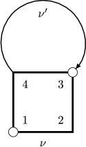
Figure 7: Feynman diagram for the first order dual fermion perturbation for the self-energy $\widetilde{\Sigma}_{12}(\nu)$: a line represents the non-local dual Green’s function $\widetilde{G}_{43}(\nu^{\prime})$ and a box is the two-particle vertex (cumulant) $\gamma_{1234}$, $(\sigma,\sigma^{\prime})$ are spin-indices.

The first order for the vertex in particle-hole (PH) channel is given by the diagram shown in Fig.7

$$\tilde{\Sigma}_{12}^{(1)}=-\sum_{s-QMC}\sum_{3,4}\gamma_{1234}^{d}(s)\tilde{G}^{0}_{34}$$ (8)

Here the density vertex in PH channel is

$$\gamma_{1234}^{d}=\gamma^{\uparrow\uparrow\uparrow\uparrow}_{1234}+\gamma^{\uparrow\uparrow\downarrow\downarrow}_{1234}$$ (9)

and the final Green’s function reads

$$G_{12}=\left[\left(g+{\tilde{\Sigma}}\right)^{-1}-\tilde{t}\right]^{-1}_{12}$$ (10)

Within the determinant DQMC with Ising-fields $\{s\}$ or inside the CT-INT with stochastic sampling of interaction order expancion $\{s\}$ for two-particle correlators we can use the Wick-theorem:

$$\gamma_{1234}(s)\equiv\langle{c_{1}^{\phantom{*}}c_{2}^{*}c_{3}^{\phantom{*}}c_{4}^{*}}\rangle_{s}=\langle{c_{1}^{\phantom{*}}c_{2}^{*}}\rangle_{s}\,\langle{c_{3}^{\phantom{*}}c_{4}^{*}}\rangle_{s}-\langle{c_{1}^{\phantom{*}}c_{4}^{*}}\rangle_{s}\,\langle{c_{3}^{\phantom{*}}c_{2}^{*}}\rangle_{s}$$ (11)

K space scheme

For large system ($N\geq 4$) it is much faster to calculate the dual self-energy in the K-space with within the QMC Markov chain. The dual action in K-space reads

$$\tilde{S}[d^{\ast},d]=-\sum_{\mathbf{k}\,\nu\sigma}d_{\mathbf{k}\nu\sigma}^{\ast}\;\tilde{G}_{0\mathbf{k}\nu}^{-1}\;d_{\mathbf{k}\nu\sigma}+\frac{1}{4}\sum_{1234}\gamma_{1234}d_{1}^{\ast}d_{2}^{\ast}d_{3}d_{4}\,.$$ (12)

Using the short notation $k\equiv(\mathbf{k},\nu_{n})$ and $\nu_{n}=(2n+1)\pi/\beta$, with $n\in\mathbb{Z}$, the dual Green’s function is equal to

$$\tilde{G}_{k}^{0}=\left(\tilde{t}_{k}^{-1}-\hat{g}_{k}\right)^{-1}\,.$$ (13)

Since the bare dual Green’s function calculated in the independent QMC run for the reference system, it is fully translationally invariant $\tilde{G}^{0}_{34}\equiv\tilde{G}^{0}(3-4)$ and we used Fourier transform to calculate the K-space dual Green’s function $\tilde{G}^{0}_{k}$.

Within the QMC Markov chain the lattice auxilary Green’s function is not translationally invariant therefore $g^{s}_{12}=-\langle c_{1}c_{2}^{\ast}\rangle_{s}$ and we use double Fourier transform to calculate $g^{s}_{kk^{\prime}}$. To include ”disconnected part” of the vertex in equation Eq. (7) we just substract exact Green’s function from the previus QMC run of the reference system as following

$$\tilde{g}^{s}_{12}=g^{s}_{12}-g_{12}$$ (14)

In the K-space this subtractions has the following form

$$\tilde{g}^{s}_{kk^{\prime}}=g^{s}_{kk^{\prime}}-g_{k}\delta_{kk^{\prime}}$$ (15)

For transformation of the vertex $\gamma_{1234}^{d}$ in Eq. (9)within the QMC step in the K-space we take into account that indices $3,4$ are ”diagonal” in $k$-spcae due to multiplication by translationally invariant dual Green’s function $\tilde{G}^{0}_{34}$ which transforms as $\tilde{G}^{0}_{k}\delta_{kk^{\prime}}$ and indices $1,2$ become translationally invariant after QMC-summation, which finally leads us to the following equation for final spin-up components of the first order dual self-energy $\tilde{\Sigma}_{k}$

$$\tilde{\Sigma}_{k}^{(1)}=\frac{-1}{(\beta N)^{2}Z_{QMC}}\sum_{s-QMC}\sum_{k^{\prime}}\left[\tilde{g}_{kk}^{\uparrow\uparrow}\tilde{g}_{k^{\prime}k^{\prime}}^{\uparrow\uparrow}-\tilde{g}_{kk^{\prime}}^{\uparrow\uparrow}\tilde{g}_{k^{\prime}k}^{\uparrow\uparrow}+\tilde{g}_{kk}^{\uparrow\uparrow}\tilde{g}_{k^{\prime}k^{\prime}}^{\downarrow\downarrow}\right]_{s}\tilde{G}^{0}_{k^{\prime}}$$ (16)

Additional normalisation factor $\frac{1}{(\beta N)^{2}}$ comes from the Fourier transform in $k$ and from the $\mathbf{k^{\prime}}$-sum with $N$-lattice cites and summation over Matsubara frequency: $\frac{1}{\beta}\sum_{\nu^{\prime}}(...)$. For paramagnetic calculations we average over two spin projections.

Corresponding lattice Green’s function reads:

$$G_{k}=\left[\left(g_{k}+{\tilde{\Sigma}_{k}}\right)^{-1}-\tilde{t}_{k}\right]^{-1}\,.$$ (17)

Finally, we note, that if we neglect the dual self-energy, $\tilde{\Sigma}_{k}=0$, this approximation is equivalent to so-called cluster-perturbation theory (CPT) for $N\times N$ system Valenti_CPT .

Supplementary Note 1. Periodization of bare Green’s Function

For calculation of a bare Green’s function for $N\times N$ system we used a special scheme to reduce dependence on the cluster size. We start from the non-interacting Green’s function with given $t^{\prime}/t$ and $\mu$ for a infinite lattice (in practice $50N\times 50N$ with periodic boundary condition). Then we cut the Green’s function to only our small system $N\times N$ which results in non-periodic Green’s function ${\cal G}_{ij}(\nu_{n})$ with (i,j=0,N-1). In order to periodize the Green’s function for small system we average corresponding distance, for example ${\cal G}_{0,n}$ and ${\cal G}_{0,N/2-n}$. In practice, we used ”double” Fourie transform on $i$ and $j$ from ${\cal G}_{ij}$ to ${\cal G}_{kk^{\prime}}$ and take the diagonal (periodic) part ${\cal G}_{k}\delta_{kk^{\prime}}$. In this way the local Green’s function does not depends on the size of our cluster (Supplementary Figure 1a) and the non-local part (Supplementary Figure 1b) has much faster converge in comparisson to standard periodic DCA cluster scheme DCA_RMP . The reason for this fast convergence of the non-local Green’s function and exact local Green’s function related with real space periodization, while DCA make the average patches in the K-space.

Supplementary Figure 1. Periodized Green’s function in imaginary time $\tau$ for clusters $N\times N$ with $N=2,4,8$ for our scheme compare to DCA approach for the reference system with $U=5.56$ $t^{\prime}=0$ and $\mu=0$ for $\beta=10$. The local Green’s function (left) and first nearest-neighbours (right).

Supplementary Note 2. Tests for the $2\times 2$ system

For the smallest $2\times 2$ we can use a very transparent real-space DF-QMC algorithm. In this case we do not need any additional periodization since $2\times 2$ cluster is “self-periodic”. Since there is almost no sign problem in DQMC method for the doped $2\times 2$ cluster in the bath, we can compare the first-order dual-fermion perturbation with numerical exact DQMC results. The all three non-equivalent Green’s functions for $2\times 2$ system are shown in the Supplementary Figure 2 using first-order DF-correction within Hirsch-Fye QMC formalism. For small perturbation $\Delta\mu=-0.3$ and $\Delta t^{\prime}=0$ a comparison with exact DQMC results (point on Supplementary Figure 2) is perfect. For a large perturbation $\Delta\mu=-1.5$ and $\Delta t^{\prime}=0.15$ one can already see a small difference from the exact DQMC Green’s function. Nevertheless, the results of DF-QMC with only first-order corrections for the dual self-energy are very satisfactory. Note that for square lattice the perturbation in $\Delta\mu$ one can compare with $4\Delta t^{\prime}$, also dispersion of $t^{\prime}$ terms made this estimation questionable.

Supplementary Figure 2. Three non-equivalent components of the Green’s functions for $2\times 2$ system as function of imaginary time for $U=5.56$, $\beta=5$ and $t^{\prime}/t=-0.1$, $\mu=0$ (left) and $t^{\prime}/t=-0.3$, $\mu=-1.3$ (right). Notes, that here we use a QMC defitition with positive local Green’s function.

Supplementary Note 3.: Tests for the $4\times 4$ system

Supplementary Figure 3. Green’s functions from DF-QMC (DFQ) in comparison with numerically exact DQMC result (QMC) for the (4 $\times$ 4) system in Matsubara space with $U=5.56$, $t^{\prime}/t=-0.1$, $\mu=0$ and $\beta=5$, real par (left) and imaginary part (right).

Supplementary Figure 4. Green’s functions from DF-QMC (DFQ) in comparison with numerically exact DQMC result (QMC) for the (4 $\times$ 4) system in Matsubara space with $U=5.56$, $t^{\prime}/t=-0.3$, $\mu=0$ and $\beta=5$, real par (left) and imaginary part (right).

Supplementary Figure 5. Green’s functions from DF-QMC (DFQ) in comparison with numerically exact DQMC result (QMC) for the (4 $\times$ 4) system in Matsubara space with $U=5.56$, $t^{\prime}/t=0$, $\mu=-0.5$ and $\beta=5$, real par (left) and imaginary part (right).

We analyse performance of DF-QMC formalism as function of $\Delta\mu$ and $\Delta t^{\prime}$ for the 4 $\times$ 4 periodic cluster with and without fernionic bath. The DQMC sign problem for 4 $\times$ 4 system is also mild and we can compare our DF-QMC with numerically exact test for the same $\mu$ and $t^{\prime}$. We use value of $U=5.56$ which corresponds to the degenerate ground state of plaquete danilov2022 . For all Hirsch-Fye DQMC calculations we use imaginary time discretisation with $L=64$ slices. Supplementary Figure 3 shows DF-QMC results for a small perturbation $t^{\prime}/t=-0.1$ and $\beta=5$ in comparison with exact DQMC results. The agreement is very good which show the strength dual fermion QMC theory. for a small perturbation. Next, we compare Supplementary Figure 4 for the $t^{\prime}/t=-0.3$ case which corresponds to optimal next-nearest hopping in cuprate materials. In this case one can see the difference from exact DQMC results on the first Matsubara frequency, but still the overall agreement in all 6 nonequilibrium k-points for 4 $\times$ 4 system is quite satisfactory.

The effects of chemical potential shift $\mu=-0.5$ presented on Supplementary Figure 5. Qualitatively, agreement between perturbative DF-QMC and exact DQMC is similar to the case of $t^{\prime}/t=-0.3$, but the structure of all 6 Green’s functions for $4\times 4$ system is very different and still the dual-fermion strong coupling perturbation in K-space works reasonably well.

Finally, Supplementary Figure 6, shows the combine effects of strong chemical potential shift $\mu=-1$ and next-nearest hopping $t^{\prime}/t=-0.3$. In this case we shows results of the CT-INT approach with $\beta=10$ The agreement is very good, and only one Green’s function (the lowest imaginary part) which corresponds to $X$-point ${\bf k}=(\pi,\pi)$ and located close to the Fermi level (corresponding real part is close to zero) the dual perturbation shows small discrepancy. In principle, one can reduce the error of dual perturbation if one can choose the reference more close to the target system. The main condition is a weak sign problem for the reference system. Since it is always the case for small $4\times 4$ cluster, we show in the Supplementary Figure 7 the CT-INT results of reference system corrrsponding to $t^{\prime}/t=-0.1$ for the target system of $t^{\prime}/t=-0.3$. In this case, for lower temperature $T=t/10$ the DF-QMC resalts are still in a good agreement with exact solution.

Supplementary Figure 6. Green’s functions from DF-CT-QMC (DF-QMC) in comparison with numerically exact QMC result (CT-QMC) for the (4 $\times$ 4) system in Matsubara space with $U=5.56$, $t^{\prime}/t=-0.3$, $\mu=-1$ and $\beta=10$, real par (left) and imaginary part (right).

Supplementary Figure 7. Green’s functions from DF-CT-QMC (DF-QMC) perturbation for $t^{\prime}/t=-0.3$, starting from the reference system with $t^{\prime}/t=-0.1$ in comparison with numerically exact QMC result (CT-QMC) for the (4 $\times$ 4) system in Matsubara space with $U=5.56$, $\mu=0$ and $\beta=10$, real par (left) and imaginary part (right).

Supplementary Figure 8. Green’s function for the (8 $\times$ 8) for $U=5.56$, $t^{\prime}/t=-0.3$, $\mu=-1.5$ $\beta=3$ for Hirsch-Fye DF-QMC (DFQ) in comparisson with DQMC test (QMC).

Supplementary Figure 9. Green’s functions within Hirsch-Fye DF-QMC scheme for 15 nonequivalent $\bf k$-points of the (8 $\times$ 8) cluster in the bath with $U=8$, $\mu=-2$, $t^{\prime}/t=-0.3$ and $\beta=10$

Supplementary Figure 10. The Fermi surface calculating within Hirsch-Fye DF-QMC scheme forthe (8 $\times$ 8) cluster in the bath with $U=8$, $\mu=-2$, $t^{\prime}/t=-0.3$ and $\beta=10$.

Supplementary Note 4.: Tests for the $8\times 8$ system

For large $8\times 8$ system for $\beta=10$ the average sign in DQMC is of the order of a $10^{-3}$ even with a fermionic bath and calculation of the test Green’s function is not any more possible. For much larger temperature, corresponds to $\beta=3$ and not so large $U=5.5.6$ the sign problem is not severe and it is still possible to prepare a DQMC test. Supplementary Figure 8 shows a comparison of Matsubara Green’s function for all 15 non-equivalent $\bf k$-points im dual-fermion perturbation with Hirsch-Fye QMC code and DQMC-test. The agreement is quite good, but one should remember a very high temperature of this test ($T=t/3$) which results in metallic behaviour of all Green’s functions. We also present the Green’s functions for the same parameters as in the main text, but using the Hirsch-Fye QMC schem for $8\times 8$ system (Supplementary Figure 9) and corresponding Fermi surface (Supplementary Figure 10). There is a good agreement with CT-INT scheme in the main text, and if we take into account very different computational scheme for these two methods, we can state that ”as proof of principle” the DF-QMC approach can efficiently overcome the sign problem in the lattice DQMC approach for doped systems with long-range hoppings.

The authors thank Alexei Rubtsov, Evgeny Stepanov, Igor Krivenko, Jörg Schmalian, Richard Scalettar, Emanuel Gull, Fedor Šimkovic IV, Riccardo Rossi and Antoine Georges for valuable comments on the work.

This work was partially supported by the Cluster of Excellence “Advanced Imaging of Matter” of the Deutsche Forschungsgemeinschaft (DFG) - EXC 2056 - Project No. ID390715994, by European Research Council via Synergy Grant 854843 - FASTCORR. The part of simulations were performed on the national supercomputer HPE Apollo Hawk at the High Performance Computing Center Stuttgart (HLRS) under the grant number QMCdynCOR/44167. User Facility supported by the Office of Science of the U.S. Department of Energy under Contract No. DE-AC02-05CH11231 using NERSC award BES-ERCAP0020359.

References

- (1) Schäfer, T. et al. Tracking the footprints of spin fluctuations: A multimethod, multimessenger study of the two-dimensional Hubbard model. Phys. Rev. X 11, 011058 (2021). https://link.aps.org/doi/10.1103/PhysRevX.11.011058.
- (2) De Raedt, H. & Lagendijk, A. Monte Carlo simulation of quantum statistical lattice models. Physics Reports 127, 233–307 (1985). https://www.sciencedirect.com/science/article/pii/0370157385900444.
- (3) Loh, E. Y. et al. Sign problem in the numerical simulation of many-electron systems. Phys. Rev. B 41, 9301–9307 (1990). https://link.aps.org/doi/10.1103/PhysRevB.41.9301.
- (4) Troyer, M. & Wiese, U.-J. Computational complexity and fundamental limitations to fermionic quantum monte carlo simulations. Phys. Rev. Lett. 94, 170201 (2005). https://link.aps.org/doi/10.1103/PhysRevLett.94.170201.
- (5) Mondaini, R., Tarat, S. & Scalettar, R. T. Quantum critical points and the sign problem. Science 375, 418–424 (2022). https://www.science.org/doi/abs/10.1126/science.abg9299. eprint https://www.science.org/doi/pdf/10.1126/science.abg9299.
- (6) Jiang, H.-C. & Devereaux, T. P. Superconductivity in the doped Hubbard model and its interplay with next-nearest hopping t’. Science 365, 1424–1428 (2019). https://science.sciencemag.org/content/365/6460/1424. eprint https://science.sciencemag.org/content/365/6460/1424.full.pdf.
- (7) Jiang, Y.-F., Zaanen, J., Devereaux, T. P. & Jiang, H.-C. Ground state phase diagram of the doped Hubbard model on the four-leg cylinder. Phys. Rev. Res. 2, 033073 (2020). https://link.aps.org/doi/10.1103/PhysRevResearch.2.033073.
- (8) Chung, C.-M., Qin, M., Zhang, S., Schollwöck, U. & White, S. R. Plaquette versus ordinary -wave pairing in the -Hubbard model on a width-4 cylinder. Phys. Rev. B 102, 041106 (2020). https://link.aps.org/doi/10.1103/PhysRevB.102.041106.
- (9) Qin, M. et al. Absence of superconductivity in the pure two-dimensional Hubbard model. Phys. Rev. X 10, 031016 (2020). https://link.aps.org/doi/10.1103/PhysRevX.10.031016.
- (10) Harland, M., Katsnelson, M. I. & Lichtenstein, A. I. Plaquette valence bond theory of high-temperature superconductivity. Phys. Rev. B 94, 125133 (2016). https://link.aps.org/doi/10.1103/PhysRevB.94.125133.
- (11) Harland, M., Brener, S., Katsnelson, M. I. & Lichtenstein, A. I. Exactly solvable model of strongly correlated -wave superconductivity. Phys. Rev. B 101, 045119 (2020). https://link.aps.org/doi/10.1103/PhysRevB.101.045119.
- (12) Danilov, M. et al. Degenerate plaquette physics as key ingredient of high-temperature superconductivity in cuprates. npj Quant. Mater. 7, 50 (2022). https://www.nature.com/articles/s41535-022-00454-6.
- (13) Prokof’ev, N. & Svistunov, B. Bold diagrammatic monte carlo technique: When the sign problem is welcome. Phys. Rev. Lett. 99, 250201 (2007). https://link.aps.org/doi/10.1103/PhysRevLett.99.250201.
- (14) Rossi, R. Determinant diagrammatic monte carlo algorithm in the thermodynamic limit. Phys. Rev. Lett. 119, 045701 (2017). https://link.aps.org/doi/10.1103/PhysRevLett.119.045701.
- (15) Rubtsov, A. N., Savkin, V. V. & Lichtenstein, A. I. Continuous-time quantum Monte Carlo method for fermions. Phys. Rev. B 72, 035122 (2005). https://link.aps.org/doi/10.1103/PhysRevB.72.035122.
- (16) Šimkovic, F., 2Rossi, R., Georges, A. & Ferrero1, M. Incoherent transport across the strange metal regime of highly overdoped cuprates (2022). https://doi.org/10.48550/arXiv.2209.09237. eprint 2209.09237.
- (17) Šimkovic, F., Rossi, R. & Ferrero, M. Two-dimensional Hubbard model at finite temperature: Weak, strong, and long correlation regimes. Phys. Rev. Res. 4, 043201 (2022). https://link.aps.org/doi/10.1103/PhysRevResearch.4.043201.
- (18) Rossi, R., Prokof’ev, N., Svistunov, B., Houcke, K. V. & Werner, F. Polynomial complexity despite the fermionic sign. Europhysics Letters 118, 10004 (2017). https://dx.doi.org/10.1209/0295-5075/118/10004.
- (19) Kim, A. J., Prokof’ev, N. V., Svistunov, B. V. & Kozik, E. Homotopic action: A pathway to convergent diagrammatic theories. Phys. Rev. Lett. 126, 257001 (2021). https://link.aps.org/doi/10.1103/PhysRevLett.126.257001.
- (20) Charlebois, M. & Imada, M. Single-particle spectral function formulated and calculated by variational monte carlo method with application to -wave superconducting state. Phys. Rev. X 10, 041023 (2020). https://link.aps.org/doi/10.1103/PhysRevX.10.041023.
- (21) Rosenberg, P., Sénéchal, D., Tremblay, A.-M. S. & Charlebois, M. Fermi arcs from dynamical variational Monte Carlo. Phys. Rev. B 106, 245132 (2022). https://link.aps.org/doi/10.1103/PhysRevB.106.245132.
- (22) Sakai, S., Civelli, M. & Imada, M. Hidden fermionic excitation boosting high-temperature superconductivity in cuprates. Phys. Rev. Lett. 116, 057003 (2016). https://link.aps.org/doi/10.1103/PhysRevLett.116.057003.
- (23) Singh, A. et al. Unconventional exciton evolution from the pseudogap to superconducting phases in cuprates. Nature Communications 13, 7906 (2022). https://doi.org/10.1038/s41467-022-35210-8.
- (24) Krien, F., Worm, P., Chalupa-Gantner, P., Toschi, A. & Held, K. Explaining the pseudogap through damping and antidamping on the fermi surface by imaginary spin scattering. Communications Physics 5, 336 (2022). https://doi.org/10.1038/s42005-022-01117-5.
- (25) Brener, S., Stepanov, E. A., Rubtsov, A. N., Katsnelson, M. I. & Lichtenstein, A. I. Dual fermion method as a prototype of generic reference-system approach for correlated fermions. Annals of Physics 422, 168310 (2020). http://www.sciencedirect.com/science/article/pii/S000349162030244X.
- (26) Abrikosov, A. A., Gorkov, L. P. & Dzyaloshinski, I. E. Methods of quantum field theory in statistical physics (Dover, New York, NY, 1975). https://cds.cern.ch/record/107441.
- (27) Georges, A., Kotliar, G., Krauth, W. & Rozenberg, M. J. Dynamical mean-field theory of strongly correlated fermion systems and the limit of infinite dimensions. Rev. Mod. Phys. 68, 13–125 (1996). https://link.aps.org/doi/10.1103/RevModPhys.68.13.
- (28) Rubtsov, A. N., Katsnelson, M. I. & Lichtenstein, A. I. Dual fermion approach to nonlocal correlations in the Hubbard model. Phys. Rev. B 77, 033101 (2008). http://link.aps.org/doi/10.1103/PhysRevB.77.033101.
- (29) Bethe, H. A. & Jackiw, R. W. Intermediate quantum mechanics (3rh edition) (Taylor and Francis, London, 1986). https://www.taylorfrancis.com/books/mono/10.1201/9780429493645/intermediate-quantum-mechanics-roman-jackiw.
- (30) Katsnelson, M. I. & Irkhin, V. Y. Metal-insulator transition and antiferromagnetism in the ground state of the Hubbard model. J. Phys. C 17, 4291–4308 (1984). https://iopscience.iop.org/article/10.1088/0022-3719/17/24/011.
- (31) Irkhin, V. Y. & Katsnelson, M. I. On the ground state wave function of a superconductor in the BCS model. Phys. Lett. A 104, 163–165 (1984). https://www.sciencedirect.com/science/article/pii/0375960184903682.
- (32) Irkhin, V. Y. & Katsnelson, M. I. Theory of intermediate-valence semiconductors. Sov. Phys. JETP 63, 631–636 (1986). http://www.jetp.ras.ru/cgi-bin/e/index/e/63/3/p631?a=list.
- (33) Peierls, R. On a Minimum Property of the Free Energy. Phys. Rev. 54, 918–919 (1938). https://link.aps.org/doi/10.1103/PhysRev.54.918.
- (34) Feynman, R. P. Statistical mechanics: A set of lectures (Reading, Mass: Benjamin/Cummings, 1972).
- (35) Bogolyubov, N. N. On a variational principle in the many-body problem. Sov. Phys. Dokl. 3, 292–294 (1958).
- (36) Scalettar, R. T., Noack, R. M. & Singh, R. R. P. Ergodicity at large couplings with the determinant monte carlo algorithm. Phys. Rev. B 44, 10502–10507 (1991). https://link.aps.org/doi/10.1103/PhysRevB.44.10502.
- (37) Rohringer, G. et al. Diagrammatic routes to nonlocal correlations beyond dynamical mean field theory. Rev. Mod. Phys. 90, 025003 (2018). https://link.aps.org/doi/10.1103/RevModPhys.90.025003.
- (38) Rost, D., Gorelik, E. V., Assaad, F. & Blümer, N. Momentum-dependent pseudogaps in the half-filled two-dimensional Hubbard model. Phys. Rev. B 86, 155109 (2012). https://link.aps.org/doi/10.1103/PhysRevB.86.155109.
- (39) Fei, J., Yeh, C.-N., Zgid, D. & Gull, E. Analytical continuation of matrix-valued functions: Carathéodory formalism. Phys. Rev. B 104, 165111 (2021). https://link.aps.org/doi/10.1103/PhysRevB.104.165111.
- (40) Hirsch, J. E. & Fye, R. M. Monte carlo method for magnetic impurities in metals. Phys. Rev. Lett. 56, 2521–2524 (1986). https://link.aps.org/doi/10.1103/PhysRevLett.56.2521.
- (41) Wu, W., Ferrero, M., Georges, A. & Kozik, E. Controlling feynman diagrammatic expansions: Physical nature of the pseudogap in the two-dimensional Hubbard model. Phys. Rev. B 96, 041105 (2017). https://link.aps.org/doi/10.1103/PhysRevB.96.041105.
- (42) Rossi, R., Šimkovic, F. & Ferrero, M. Renormalized perturbation theory at large expansion orders. EPL (Europhysics Letters) 132, 11001 (2020). https://doi.org/10.1209/0295-5075/132/11001.
- (43) Hafermann, H., Brener, S., Rubtsov, A. N., Katsnelson, M. I. & Lichtenstein, A. I. Cluster dual fermion approach to nonlocal correlations. JETP Letters 86, 677–682 (2008). https://doi.org/10.1134/S0021364007220134.
- (44) Pairault, S., Sénéchal, D. & Tremblay, A.-M. S. Strong-coupling expansion for the Hubbard model. Phys. Rev. Lett. 80, 5389–5392 (1998). https://link.aps.org/doi/10.1103/PhysRevLett.80.5389.
- (45) Gros, C. & Valentí, R. Cluster expansion for the self-energy: A simple many-body method for interpreting the photoemission spectra of correlated fermi systems. Phys. Rev. B 48, 418–425 (1993). https://link.aps.org/doi/10.1103/PhysRevB.48.418.
- (46) Maier, T., Jarrell, M., Pruschke, T. & Hettler, M. H. Quantum cluster theories. Rev. Mod. Phys. 77, 1027–1080 (2005). https://link.aps.org/doi/10.1103/RevModPhys.77.1027.