Time-inconsistent contract theory

Abstract

This paper investigates the moral hazard problem in finite horizon with both continuous and lump-sum payments, involving a time-inconsistent sophisticated agent and a standard utility maximiser principal. Building upon the so-called dynamic programming approach in Cvitanić, Possamaï, and Touzi [18] and the recently available results in Hernández and Possamaï [43], we present a methodology that covers the previous contracting problem. Our main contribution consists in a characterisation of the moral hazard problem faced by the principal. In particular, it shows that under relatively mild technical conditions on the data of the problem, the supremum of the principal’s expected utility over a smaller restricted family of contracts is equal to the supremum over all feasible contracts. Nevertheless, this characterisation yields, as far as we know, a novel class of control problems that involve the control of a forward Volterra equation via Volterra-type controls, and infinite-dimensional stochastic target constraints. Despite the inherent challenges associated to such a problem, we study the solution under three different specifications of utility functions for both the agent and the principal, and draw qualitative implications from the form of the optimal contract. The general case remains the subject of future research.

Key words: Moral hazard, time-inconsistency, consistent planning, sophisticated agent, dynamic utilities, backward stochastic Volterra integral equations, stochastic target.

In this paper, we are interested in the moral hazard contracting problem between a principal and an agent with time-inconsistent preferences. A principal–agent problem pertains to the optimal contracting between two parties: the principal, who is interested in hiring the agent, offers a contract; provided the agent accepts, he can influence a random process, the outcome, via his actions. A key feature in these models is the amount of information available to the principal when designing the contract. There are three classical cases studied in the literature: risk-sharing with symmetric information, hidden action, and hidden type. We are only concerned with the first two in this work.

In the risk-sharing scenario, also referred to as the first-best, both parties have the same information and have to agree on how to share the underlying risk. The principal thus has all the bargaining power, i.e. she offers the contract and dictates the agent’s actions—the agent is compelled to follow or else he would be severely penalised. In the case of hidden actions, the principal is imperfectly informed about the agent’s actions. Either they are too costly to be monitored or simply unobservable. Consequently, the principal expects to receive a second-best utility compared to the risk-sharing case. As the agent is allowed to take actions that are not in the principal’s best interest, this situation is also referred to as moral hazard, and incentives play a crucial role. Indeed, the principal hopes to influence the agent’s actions by offering an appropriate contract.

In the case of a traditional (time-consistent) agent, a common feature of these models is that their resolution boils down to standard stochastic control theory. Indeed, in light of the principal’s bargaining power, the first-best case is always cast as a stochastic control problem for a single individual—the principal—who chooses both the contract and the actions under the participation constraint. On the other hand, in the second-best problem, it being a two-stage Stackelberg game, one has to solve the agent’s problem for any given fixed contract before moving to study the principal’s problem. In principle, this creates a much more complicated structure on the problem. Since the introduction of the continuous-time model, it took time for the literature to present a general approach that arrived at the same conclusion for the second-best problem.

The study of moral hazard problems in continuous time has its roots in the seminal paper of Holmström and Milgrom [45]. In this model, the principal and the agent have CARA utility functions, and the agent’s effort influences the drift of the output process, the solution to a controlled diffusion, but not the volatility. The resulting optimal contract is a linear function of the aggregate output. The model in [45] drew great attention as the resolution of the, seemingly more complicated, continuous-time formulation was actually much more tractable, could be rigorously justified, and provided useful explicit solutions for the economic analysis. These were typically harder to reach in most of the discrete-time models that dominated the existing literature, see Laffont and Martimort [49] for an overview. Following upon [45], Schättler and Sung [71, 72] studied the validity of the so-called first-order approach, while Sung [78, 79] provided extensions to the case of diffusion control and hierarchical structures. The linearity of the optimal contract, a feature also present in [78], is further studied in Müller [62, 63], Hellwig and Schmidt [40], Hellwig [39] and Sung [80, 81] for the first-best problem, the interplay between the discrete-time and continuous-time models, and for a robust setting, respectively. Notably, Williams [90] and Cvitanić, Wan, and Zhang [16] characterise the optimal contract for general utilities by means of the so-called stochastic maximum principle and forward–backward stochastic differential equations (FBSDEs for short).

Nevertheless, it was not until the approach in Sannikov [68, 69] was available that the study of the moral hazard problem was, once again, reinvigorated and arrived finally at the methodical program presented in Cvitanić, Possamaï, and Touzi [17, 18]. In a nutshell, this method leverages the dynamic programming principle and the theory of backward stochastic differential equations (BSDEs) to reformulate the principal’s problem as a standard optimal stochastic control problem with an additional state variable, namely, the agent’s continuation utility. This methodology has been extended to several scenarii including random horizon contracting Lin, Ren, Touzi, and Yang [55], ambiguity features from the point of view of the principal, as in Mastrolia and Possamaï [60] and Hernández Santibáñez and Mastrolia [44], a principal contracting a finite number of agents Élie and Possamaï [25], several principals contracting a common agent Mastrolia and Ren [61], a principal contracting a mean-field of agents [26], and applications in optimal electricity demand response contracting Aïd, Possamaï, and Touzi [2], or Élie, Hubert, Mastrolia, and Possamaï [27]. The road map suggested by this approach is quite clear: $(i)$ identify the generic dynamic programming representation of the agent’s value process, $(ii)$ express the contract payment in terms of the value process, $(iii)$ optimise the principal’s objective over such payments.

All in all, the previous literature is particular to the contracting problem between two (or more) standard utility maximisers, while there is a growing need for the development of models able to explain the behaviour of agents that fail to comply with classical rationality assumptions. Indeed, there is clear evidence of such attitudes in a number of applications, from consumption problems to finance, from crime to voting, and from charitable giving to labour supply, see Rabin [67] and Dellavigna [19] for detailed reviews. The distinctive feature in these situations is that human beings do not necessarily behave as perfectly rational decision-makers. In reality, their criteria for evaluating their well-being are, in many cases, a lot more involved than the ones considered in the classic literature. In light of the methodology introduced in [18], the recently available results in Hernández and Possamaï [43] unveil the possibility of extending this blueprint to cover the moral hazard problem between a principal and a sophisticated time-inconsistent agent. This is the task we seek to accomplish in this paper.

Time-inconsistency is, in general terms, the fact that marginal rates of substitution between goods consumed at different dates change over time, see Strotz [77], Laibson [50], O’Donoghue and Rabin [64, 65]. For example, the marginal rate of substitution between immediate consumption and some later consumption is different from when these two dates were seen from a remote prior date. In many applications, this introduces a conflict between ‘an impatient present self and a patient future self’, see Brutscher [11]. In mathematical terms, this translates into stochastic control problems in which the classic dynamic programming principle, or in other words, the Bellman optimality principle is not satisfied.

Time-inconsistency was first mentioned in [77] where three different types of agents are described: the pre-committed agent does not revise his initially decided strategy; the naive agent revises his strategy without taking future revisions into account; the sophisticated agent revises his strategy taking possible future revisions into account, and by avoiding such makes his strategy time-consistent. The comprehensive study of sophisticated agents started with Ekeland and Pirvu [23], see also Ekeland and Lazrak [21, 22], which later became the starting point of the general Markovian theory developed by Björk, Khapko, and Murgoci [7]. Nonetheless, none of these approaches could handle the typical non-Markovian problems that would necessarily arise in contracting problems involving a principal and a time-inconsistent agent. Hernández and Possamaï [43] provided a probabilistic formulation able to accommodate a general non-Markovian structure and provided an extended dynamic programming principle (DPP) for a refinement of the notion of equilibria first introduced in [22]. In turn, the extended DPP leads to the introduction of a system of BSDEs analogous to the classical HJB equation. This system is fundamental in the sense that its well-posedness is both necessary and sufficient to characterise the value function and equilibria, which are identified as maximisers of the Hamiltonian.

When it comes to incorporating time-inconsistent features into contract theory models, the economic literature is abundant in discrete-time models with two and up to three periods. A common feature in this literature is adopting quasi-hyperbolic discounting structures to draw conclusions in different mechanism design problems. Yet, the method of resolution in each problem remained limited to a case-by-case analysis. For instance, Amador, Werning, and Angeletos [4] and Bond and Sigurdsson [8] study the feasibility of commitment in models of consumption and savings, whereas Galperti [31] considers the optimal provision of commitment devices to people who value both commitment and flexibility. Bisin, Lizzeri, and Yariv [6] examines policymakers’ responses to the political demands of agents with self-control problems, Halac and Yared [34] looks into a fiscal policy model in which the government has time-inconsistent preferences, while Lim and Yurukoglu [54] assesses the effects of time-inconsistency on monopoly regulation of electricity distribution. Heidhues [38] and Karaivanov and Martin [47] integrate time-inconsistent preferences into credit, mortgage, and insurance contract design problems, respectively. Englmaier, Fahn, and Schwarz [28], Gottlieb [32] and Gottlieb and Zhang [33] study contracting problems between firms and sophisticated, partially naive, and naive present-biased consumers. Yılmaz [91, 92] considers a repeated moral hazard problem involving a sophisticated and naive agent, respectively. Ma [58] studies a multi-period model in which contracts are subject to renegotiations, and the agent’s action has a long-term effect. Balbus, Reffett, and Wozny [5] shows the existence of time-consistent equilibria for dynamic models with generalised discounting. A survey of some of the state of behavioural economics research in contract theory was provided in Kószegi [48].

In continuous-time, where the dynamic models are sometimes more tractable and the solutions enjoy better interpretability, the literature becomes rather scarce. Models dealing with a pre-committed agent have been considered in Li and Qiu [52], in which a non-constant exponential discount factor is the source of time-inconsistency, and Djehiche and Helgesson [20], where the agent is allowed to have mean-variance utility functions. The case of a sophisticated agent was considered in Li, Mu, and Yang [53], Liu, Mu, and Yang [56], Liu, Huang, Liu, and Mu [57] and Wang, Huang, Liu, and Zhang [88] in the case of hyperbolic discounting. However, the time-inconsistency is restricted in the sense that it manifests only at discrete random times that are exponentially distributed. Lastly, Cetemen, Feng, and Urgun [13] considers a Markovian continuous-time contracting problem and dynamic inconsistency arising from non-exponential discounting. The authors’ examples are limited to the case of a principal having time-inconsistent preferences, and the agent having standard time-consistent preferences. Altogether, a thorough analysis of the general non-Markovian continuous-time contracting problem between a standard utility maximiser principal and a sophisticated time-inconsistent agent is still missing in the literature. This is because, in our opinion, the crux of the problem lies in identifying a proper description of the problem of the principal. In the case of a classic time-consistent agent and a time-inconsistent principal, following [18], one expects the problem of the principal to boil down to a non-Markovian time-inconsistent control problem with an additional state variable. As studied in [43], these problems are characterised by an infinite family of BSDEs, equivalent to a so-called type-I extended BSVIE [42]. As such, we expect that the problem considered in this document will open the door to a complete analysis of the problem in which both the principal and the agent are time-inconsistent.

Our results

Our problem is cast in the context of a standard utility maximiser principal and an agent with time-inconsistent preferences. Indeed, the agent’s reward is given by the value of a so-called backward stochastic Volterra integral equation. This choice of preferences for the agent allows us to cover classic separable and non-separable utilities simultaneously. As is standard in the literature, we consider the weak formulation of the problem. The state process $X$ is fixed, and the agent’s actions influence the drift of $X$ through its distribution over the interval $[0,T]$. The principal chooses a contract, i.e. a process and a random variable adapted to the filtration generated by the path $X_{\cdot\wedge T}$ of the state process, which specifies the continuous payments, the terminal payment, and satisfies the agent’s participation constraint at time $t=0$. As mentioned above, our approach is inspired by that of [18] and the recent results for non-Markovian time-inconsistent control problems from a game-theoretic point of view of [43]. Indeed, [43] established an extended dynamic programming principle for the agent’s value process associated with any equilibrium action. In turn, this result was used to establish a direct link between the agent’s problem and an infinite family of BSDEs. Following [42], such a system is actually equivalent to a so-called type-I extended BSVIE.

At this point, we notice the first stark difference between the classic time-consistent case and ours: the problem of the agent is, in general, linked to the solution of an infinite family of equations, namely the BSVIE, as opposed to one, a BSDE. Nevertheless, the agent’s preferences elucidate a connection at the terminal time $t=T$ between the terminal values of the BSVIE and the terminal payment offered by any admissible contract. This is the crucial insight in order to restrict our attention from the family of admissible contracts to a carefully tailored family of contracts for which the agent’s value process allows a dynamic programming representation capturing the Volterra nature of the agent’s reward. Extrapolating from the time-consistent case, the restricted family of contracts is defined in terms of a family of first-order sensitivities of the agent’s value process to the output. For this family of contracts, we show that the principal identifies the equilibrium action for the agent as the maximisers of the associated Hamiltonian. Nevertheless, echoing the agent’s time-inconsistent preferences, the resulting principal’s problem is, in general, far from being a standard stochastic control problem.

Our main contribution, namely Theorem 3.9, consists in a characterisation of the moral hazard problem faced by the principal and a sophisticated time-inconsistent agent. In particular, it shows that under relatively mild technical conditions on the data of the problem, the supremum of the principal’s expected utility over the restricted family of contracts is equal to the supremum over all feasible contracts. Nevertheless, this characterisation yields, as far as we know, a novel class of control problems. These problems involve the control of a forward Volterra equation via Volterra-type controls, and stochastic target constraints. One of the novel features of our result is that the dynamics of this process involves the diagonal value of both the forward Volterra process and the Volterra control, see Definition 3.5. In addition, the stochastic target constraint arises due to the time-inconsistent preferences of the agent, see (3.6) and Remark 3.7.

Despite the inherent challenges of this class of problems, we study the solution to moral hazard problem under three different specifications of utility functions for both the agent and the principal. For instance, for non-separable reward functionals, we find that if both the agent and the principal have exponential utilities functions and the agent’s reward is given by the discounted value of his utility, the problem reduces to a standard control problem, see Section 4.1 and Proposition 4.3. This is a feature that we also see in the risk-sharing (or first-best) contracting examples between the principal and a time-inconsistent agent that we present in Section 2. The second example considers a risk-neutral principal and a risk-neutral agent with separable reward functional. In this case, our analysis shows that it is possible to reduce the complexity of the problem. Indeed, we can exploit the structure of the problem to formulate an ansatz to the principal’s problem, for which we present a result in the spirit of a verification theorem, see Section 4.2 and Proposition 4.10. In the last example, we go back to the first setting, but in this case the agent’s (exponential) utility is taken on the discounted income. This simple modification highlights the intrinsic difficulties of the general case, and we are able to solve the problem of the principal for a class of contracts smaller than the one prescribed by the restricted family of contracts in Theorem 3.9, see Section 4.3 and Proposition 4.17. The general case remains the subject of future research.

Regarding the qualitative implications of our results we can mention the following:

1. from a methodological point of view, unlike in the time-consistent case, the solution to the moral hazard problem does not reduce, in general, to a standard stochastic control problem. Nevertheless, the solution to the risk-sharing problem between a utility maximiser principal and a time-inconsistent sophisticated agent does, see Section 2. This suggest a dire difference between the first-best and second-best problems as soon as the agent is allowed to have time-inconsistent preferences;

2. a second takeaway from our analysis is associated with the so-called optimality of linear contracts. These are contracts consisting of a constant part and a term proportional to the terminal value of the state process as in the seminal work of [45]. This was also the conclusion of Carroll [12] in a two-stage time-consistent model in which the principal demands robustness, in the sense of evaluating admissible contracts by their worst-case performance, over unknown actions the agent might take. Similar results we obtained by [80, 81] and [60] in the continuous-time setting. Moreover, the results in Abi Jaber and Villeneuve [1] show that the optimal contract remains linear when the output is driven by a Gaussian Volterra process (instead of Brownian motion). We study two examples that can be regarded as (time-inconsistent) variations of [45], which we refer to as discounted utility, see Section 4.1, and utility of discounted income, see Section 4.3. In the former case, by virtue of the simplicity of the source of time-inconsistency, we find that the optimal contract is linear. In the latter case, we find that the optimal contract is no longer linear unless there is no discounting (as in [45]). Our point here is that slight deviations of the model in [45] seem to challenge the virtues attributed to linear contracts, and this suggests that they would typically cease to be optimal in general for time-inconsistent agents;

3. lastly, we comment on the non-Markovian nature of the optimal contract. It is known that, beyond the realm of the model in [45], the optimal contract in the time-consistent scenario is, in general, non-Markovian in the state process $X$, see [18]. Indeed, we find the same result, see Proposition 4.10, in the case of an agent with separable time-inconsistent preferences, see Section 4.2. As such, we believe this is a manifestation of the agent’s time-inconsistent preferences.

Let us illustrate some of our results, see Section 1 for precise definitions. Fix a time horizon $T>0$ and consider a sophisticated time-inconsistent agent with risk-neutral preferences. This is, if the agent enters into a terminal payment contract $\xi$ with the principal, the agent seeks an equilibrium strategy $\alpha^{\star}\in{\cal E}({\cal C})$ according to

$${\rm V}^{\rm A}_{t}(\xi,\alpha)=\mathbb{E}^{\mathbb{P}^{\alpha}}\bigg{[}f(T-t)\xi-\frac{1}{2}\int_{t}^{T}f(s-t)\alpha_{s}^{2}\mathrm{d}s\bigg{|}\mathcal{F}_{t}\bigg{]},\text{ and, }X_{t}=x_{0}+\int_{0}^{t}\alpha_{r}{\mathrm{d}}r+B^{\alpha}_{t},\;\mathbb{P}^{\alpha}\text{\rm--a.s.}$$

The principal is a risk-neutral utility maximiser. This is, among all the admissible contracts $\xi\in{\cal C}$ of ${\cal F}^{X}_{T}$-measurable random variables satisfying the agent’s participation constraint ${\rm V}^{\rm A}_{0}(\xi,\alpha)\geq R_{0}$, she maximises

$${\rm V^{P}_{FB}}=\sup_{\xi\in{\cal C}}\mathbb{E}^{\mathbb{P}^{\alpha^{\star}}}\big{[}X_{T}-\xi\big{]}.$$

The agent is time-inconsistent in light of the general discounting function $f$ appearing in his reward. We summarise and illustrate some typical discounting models next. In all the illustrations in this section we take $T=50$.

$f(t)$	IDR
$f_{{\mathrm{e}}}(t):={\mathrm{e}}^{-\gamma t}$	$\gamma$
$f_{\rm h}(t):=(1+\alpha t)^{-\frac{\gamma}{\alpha}}$	$\frac{\gamma}{1+\alpha t}$
$f_{\rm q}(t):=(1-\beta){\mathrm{e}}^{-t(\lambda+\gamma)}+\beta{\mathrm{e}}^{-t\gamma}$	$\gamma+\frac{\lambda(1-\beta)}{(1-\beta)+\beta{\mathrm{e}}^{t\lambda}}$

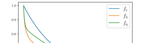
Figure 1: $(\gamma,\alpha,\lambda,\beta)\in(0,\infty)^{3}\times[0,1]$. On right graph, $\gamma_{\rm e}=0.0576,\alpha=4,\gamma_{\rm h}=1,\beta=0.7,\lambda=2.197,\gamma_{\rm q}=0.0387$.

The most widely used discounting model in classic economics is the exponential discount function $f_{\mathrm{e}}$. This model captures the empirical evidence that future utils are worth less than current utils, yet the instantaneous discount rate (IDR), given by $-f^{\prime}(t)/f(t)$, is constant over time. To be able to accommodate the fact that consumers have both a short-run preference for instantaneous gratification and a long-run preference to act patiently, Ainslie [3] introduced the hyperbolic discounting model. Hyperbolic discounting generates the so-called self-control problem, e.g. it declines at a faster rate in the short run than in the long run, depending on the value of $\alpha$, whereas $\gamma$ plays the role of baseline discounting rate. This qualitative property is even more evident in the so-called quasi-hyperbolic discounting model $f_{\rm q}$ introduced by [50]. This model exhibits the short-run impatience of the hyperbolic model, but for long time horizons, its instantaneous discount rate resembles that of the exponential model. For this discounting, $\beta$ measures the value the agent gives to future periods, whereas $\lambda$ measures the agent’s additional valuation for present/current periods. Once again, $\gamma$ is the baseline discounting rate. We can see these observations in both the IDR column of the table to the left and the plot of the three models on the right.

Let us recall that the problem faced by an agent seeking to maximise his reward is time-consistent if and only if he discounts future utils/rewards with the exponential model. Thus, taking $f_{\rm h}$ or $f_{\rm q}$ in the above formulation leads to genuine time-inconsistent problems for which sophistication would have an inherent impact in the equilibrium actions followed by the agent under the optimal contract. In addition, it is easy to see that:

• $f_{\rm h}(t)\longrightarrow f_{\rm e}(t)$, as $\alpha\longrightarrow 0$,

• $f_{\rm q}(t)\longrightarrow f_{\rm e}(t)$, as either $\beta\longrightarrow 1$ or $\lambda\longrightarrow 0$.

For any sufficiently regular discounting model, including the ones just discussed, we find in Proposition 4.10 that the associated optimal contract is given by

$$\xi^{\star}=C(R_{0})+\int_{0}^{T}\frac{z^{\star}(t)}{f(T-t)}\mathrm{d}X_{t},$$

where $C(R_{0})$ is a constant depending on the agent’s reservation utility. The second term, however, reflects the non-Markovian nature of the terminal payment mentioned in $(iii)$ above, and it is inherently related to the non-exponential discounting structure. Conversely, whenever $f=f_{\rm e}$ the term $\frac{z^{\star}(t)}{f(T-t)}$ becomes constant, leading to the well-known optimal contract that is linear in the terminal value of the output process.

We now turn our attention to the agent’s equilibrium action under the optimal contract. We illustrate this in Figure 2 below. The three columns study the above model with $f_{\rm h}$, $f_{\rm q}$ and $f_{\rm q}$ for different values of $\alpha$, $\beta$ and $\lambda$, respectively. In light of the connection with the exponential discounting mentioned above, all columns include $f_{\rm e}(t)$ in blue, which serves as a true time-consistent baseline comparison model. The first row presents the value of the discounting functions and confirms the limits pictorially. The second row presents the associated instant discounting rates, IDR, and the last row does so for the equilibrium actions. Let us first note that the shape of the equilibrium action under exponential discounting is intuitively expected. It is convex and increasing with a shape that is inversely proportional to the exponential discounting term, this reflects that the discounted optimal effort should remain constant under the optimal strategy.

Let us first look at the case of hyperbolic discounting agents. We see that as $\alpha$ increases, along the equilibrium effort, the sophisticated agent increases its level of effort during the initial stages. In addition, the rate at which the equilibrium effort changes over time (convexity/concavity) is positive for small values of $\alpha$ and negative for large values, e.g. $\alpha_{4}$ and $\alpha_{2}$, respectively. This means that as the time-inconsistency intensifies, sophistication causes the agent to exert larger levels of effort at the initial stages of the game. This reflects how sophistication can help overcome procrastination.

We now look at the quasi-hyperbolic agent in the centre and right column. As $\beta$ decreases, the agent gives less weight to the future periods and values more present over future gratification. In other words, the time-inconsistency intensifies, and the sophisticated agent decides to postpone some effort to the future period. In this scenario, despite sophistication, the agent cannot overcome procrastination. Lastly, as $\lambda$ decreases, the agent weighs less the present period, where his time-inconsistency is more acute so that the inconsistency lessens. We nevertheless find that even though the initial effort decreases, and procrastination dominates for these decreasing values of $\lambda$, namely $\lambda_{1}$ and $\lambda_{2}$, as the agent valuation of the present gets significantly small, $\lambda_{3}$ and $\lambda_{4}$ respectively, his effort increases overcoming procrastination and reaching the time-consistent level of effort. We believe that the different behaviours on the equilibrium effort for the quasi-hyperbolic discounting can be reconciled when looking at the associated IDR plots. For $t$ fixed, the IDR is monotonically decreasing in $\beta$, whereas there are values of $t$ for which the IDR oscillates when $\lambda$ decreases.

We leave the comprehensive study of these behaviours as the subject of future research. In particular, it would be interesting to study the extension of our results to the so-called instant gratification model in Harris and Laibson [37], which implements $f_{\rm ig}$ given by $f_{\rm q}\longrightarrow f_{\rm ig}$, as $\lambda\longrightarrow\infty$, and which are beyond the scope of this document.

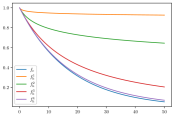
(a)

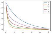
(b)

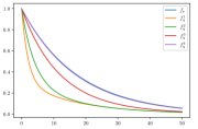
(c)

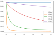
(d)

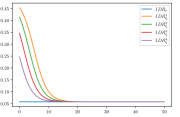
(e)

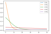
(f)

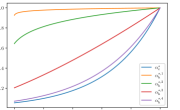
(g)

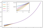
(h)

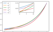
(i)

Figure 2: First row: discounting models. Second row: IDR. Third row: agent’s equilibrium action under optimal contract. $\gamma_{\rm e}=\gamma_{\rm h}=\gamma_{\rm q}=0.0575$. Left: $(\alpha_{1},\alpha_{2},\alpha_{3},\alpha_{4})=(4,0.4,0.04,0.004)$. Center: $\lambda=0.439$, $(\beta_{1},\beta_{2},\beta_{3},\beta_{4})=(0.1,0.19,0.343,0.569)$. Right: $\beta=0.3$, $(\lambda_{1},\lambda_{2},\lambda_{3},\lambda_{4})=(0.439,0.1927,0.0371,0.0013)$.

The rest of this article is organised as follows. Section 1 takes care of the formulation of the problem, and Section 2 presents the solution to the first-best problem under three different specifications of preferences. The common feature in these examples is that the problem boils down to solving a standard stochastic control problem. Section 3 introduces our general approach to the second-best problem and presents the proof of Theorem 3.9. Section 4 is devoted to the analyses of three examples under different specifications of time-inconsistent preferences for the agent. Lastly, we include an Appendix section collecting some new results for time-inconsistent control problems with BSVIE rewards and other technical results.

Notations: $\mathbb{R}_{+}$ denotes the set of non-negative real numbers. Let $(E,\|\cdot\|_{E})$ be an arbitrary finite dimensional normed space. Given a positive integer $p$ and a non-negative integer $q$, ${\cal C}_{q}(E,\mathbb{R}^{p})$ will denote the space of functions from $E$ to $\mathbb{R}^{p}$ which are at least $q$ times continuously differentiable. In the case $q=0$, of continuous functions, we drop the dependence on $q$ and write ${\cal C}([0,T],\mathbb{R}^{p})$. By $\text{I}_{n}$ we denote the identity matrix of $\mathbb{R}^{n\times n}$. $\mathbb{S}_{n}^{+}(\mathbb{R})$ denotes the set of $n\times n$ symmetric positive semi-definite matrices. ${\rm Tr}[M]$ denotes the trace of a matrix $M\in\mathbb{R}^{n\times n}$.

Let $(E,\|\cdot\|_{E})$ be an arbitrary finite dimensional normed space. For a $\sigma$-algebra ${\cal F}$, ${\cal P}_{\text{meas}}(E,{\cal F})$ denotes the space of ${\cal F}$-measurable $E$-value functions. ${\cal P}^{2}_{\text{meas}}(E,{\cal F})\big{)}$ denotes the space of $U=(U_{t}^{s})_{(s,t)\in\mathbb{R}_{+}^{2}}$ such that $(\mathbb{R}_{+}^{2}\times\Omega,{\cal B}(\mathbb{R}_{+}^{2})\otimes{\cal F})\longrightarrow({\cal B}(E),E):s\longmapsto U^{s}$ measurable. For a filtration $\mathbb{F}:=({\cal F}_{t})_{t\geq 0}$ on $(\Omega,{\cal F})$, ${\cal P}_{\rm pred}(E,\mathbb{F})$ (resp. ${\cal P}_{\rm prog}(E,\mathbb{F})$, ${\cal P}_{\rm opt}(E,\mathbb{F})$, ${\cal P}_{\rm meas}(E,\mathbb{F})$) denotes the set of $E$-valued, $\mathbb{F}$-predictable processes (resp. $\mathbb{F}$–progressively measurable processes, $\mathbb{F}$-optional processes, $\mathbb{F}$-adapted and measurable).

1 Problem statement

We fix two positive integers $n$ and $d$, which represent respectively the dimension of the process controlled by the agent, and the dimension of the Brownian motion driving this controlled process. We fix a time horizon $T>0$, and consider the canonical space $\Omega:={\cal C}([0,T],\mathbb{R}^{n})$, with canonical process $X$, and whose generic elements we denote $x$. We reserve the notation ${\rm x}$ and ${\rm\bf x}$ to denote $\mathbb{R}$-valued variables.

We let ${\cal F}$ be the Borel $\sigma$-algebra on $\Omega$ (for the topology of uniform convergence), and we denote by $\mathbb{F}^{X}:=({\cal F}^{X}_{t})_{t\in[0,T]}$ the natural filtration of $X$. We let $A$ be a compact subspace of a finite-dimensional Euclidean space (typically $A$ is a subset of $\mathbb{R}^{k}$ for some positive integer $k$), where the controls will take values.

1.1 Controlled state equation

We fix a bounded Borel measurable map $\sigma:[0,T]\times\Omega\longrightarrow\mathbb{R}^{n\times d}$, and an initial condition $x_{0}\in\mathbb{R}^{n}$, and assume that there is a unique solution, denoted by $\mathbb{P}$, to the martingale problem for which $X$ is an $(\mathbb{F}^{X},\mathbb{P})$–local martingale, such that $X_{0}=x_{0}$ with probability $1$, and $\mathrm{d}\langle X\rangle_{t}=\sigma_{t}(X_{\cdot\wedge t})\sigma^{\top}_{t}(X_{\cdot\wedge t})\mathrm{d}t$. Enlarging the original probability space if necessary (see Stroock and Varadhan [76, Theorem 4.5.2]), we can find an $\mathbb{R}^{d}$-valued Brownian motion $B$ such that

$$X_{t}=x_{0}+\int_{0}^{t}\sigma_{s}(X_{\cdot\wedge r})\mathrm{d}B_{r},\;t\in[0,T].$$

We now let $\mathbb{F}:=({\cal F}_{t})_{t\in[0,T]}$ be the $\mathbb{P}$–augmentation of $\mathbb{F}^{X}$ which we assume is right-continuous. We recall that uniqueness of the solution to the martingale problem implies that the predictable martingale representation property holds for $(\mathbb{F},\mathbb{P})$-martingales, which can be represented as stochastic integrals with respect to $X$ (see Jacod and Shiryaev [46, Theorem III.4.29]). We also mention that the right-continuity of $\mathbb{F}$ guarantees that $(\mathbb{F},\mathbb{P})$ satisfies the Blumenthal zero–one law and consequently all ${\cal F}_{0}$–measurable random variables are deterministic. Let us note that these assumptions are standard in the existing literature on the continuous-time principal–agent problem.

We can then introduce our drift functional $b:[0,T]\times\Omega\times A\longrightarrow\mathbb{R}^{d}$, which is assumed to be Borel-measurable with respect to all its arguments. Let us recall that for any $A$-valued, $\mathbb{F}$-predictable process $\alpha$ such that

$$\mathbb{E}^{\mathbb{P}}\bigg{[}\exp\bigg{(}\int_{0}^{T}b_{r}\big{(}X_{\cdot\wedge r},\alpha_{r}\big{)}\cdot\mathrm{d}B_{r}-\frac{1}{2}\int_{0}^{T}\big{\|}b_{s}\big{(}X_{\cdot\wedge s},\alpha_{r}\big{)}\big{\|}^{2}\mathrm{d}r\bigg{)}\bigg{]}<\infty,$$ (1.1)

we can define the probability measure $\mathbb{P}^{\alpha}$ on $(\Omega,{\cal F}_{T})$, whose density with respect to $\mathbb{P}$ is given by

$$\frac{\mathrm{d}\mathbb{P}^{\alpha}}{\mathrm{d}\mathbb{P}}:=\exp\bigg{(}\int_{0}^{T}b_{r}\big{(}X_{\cdot\wedge r},\alpha_{r}\big{)}\cdot\mathrm{d}B_{r}-\frac{1}{2}\int_{0}^{T}\big{\|}b_{r}\big{(}X_{\cdot\wedge r},\alpha_{r}\big{)}\big{\|}^{2}{\mathrm{d}}r\bigg{)}.$$

Moreover, by Girsanov’s theorem, the process $B^{\alpha}:=B-\int_{0}^{\cdot}b_{r}(X_{\cdot\wedge r},\alpha_{r})\mathrm{d}r$ is an $\mathbb{R}^{d}$-valued, $(\mathbb{F},\mathbb{P}^{\alpha})$–Brownian motion and we have

$$X_{t}=x_{0}+\int_{0}^{t}\sigma_{r}(X_{\cdot\wedge r})b_{r}(X_{\cdot\wedge r},\alpha_{r}){\mathrm{d}}r+\int_{0}^{t}\sigma_{r}(X_{\cdot\wedge r})\mathrm{d}B^{\alpha}_{r},\;t\in[0,T],\;\mathbb{P}\text{\rm--a.s.}$$

Let us emphasise that we are working under the so-called weak formulation of the problem. This means that the state process $X$ is fixed and, in contrast to the typical strong formulation, the Brownian motion, and the probability measure are not fixed. Indeed, the choice of $\alpha$ corresponds to the choice of probability measure $\mathbb{P}^{\alpha}$ and thus impacts the distribution of process $X$.

1.2 The agent’s problem

We aim to cover various specifications of time-inconsistent utility functions for the agent. To motivate our formulation, let us start with an informal discussion on the typical nature of the reward functionals assigned to the agent in contract theory. A contract ${\cal C}$ consists of a tuple $(\pi,\xi)$, where $\pi$ belongs the set of $\mathbb{F}$-predictable processes, and $\xi$ is a ${\cal F}_{T}$-measurable random variable. At the intuitive level, a contract consists of a flow of continuous payments $\pi:=(\pi_{t})_{t\in[0,T)}$, and a terminal compensation $\xi$. The class of admissible contracts $\Xi$ is introduced later in Section 1.3 after imposing some integrability requirements.

Given a contract ${\cal C}$ the value received by a time-inconsistent agent at the beginning of the problem from choosing an action $\alpha$ typically takes the form

$${\rm V}^{\rm A}_{0}({\cal C},\alpha):=\mathbb{E}^{\mathbb{P}^{\alpha}}\big{[}{\rm U}_{\rm A}(0,\xi,C_{0,T}^{\alpha})\big{]},\;\text{with}\;C_{t,T}^{\alpha}:=\int_{t}^{T}c_{r}(t,X_{\cdot\wedge r},\pi_{r},\alpha_{r}){\mathrm{d}}r,$$

where ${\rm U}_{\rm A}:[0,T]\times\mathbb{R}\times\mathbb{R}\longrightarrow\mathbb{R},(t,{\rm x},{\rm c})\longmapsto{\rm U}_{\rm A}(t,{\rm x},{\rm c})$ denotes the agent’s utility function and $C_{t,T}^{\alpha}$ denotes the cumulative net cost functional. We highlight that the generic dependence of both ${\rm U}_{\rm A}$ and $c$ on $t$ accounts for the sources of time-inconsistency. In the classic literature, utilities are usually classified under two categories, namely

1. separable utility functions, i.e. ${{\rm U}_{\rm A}}(t,{\rm x},{\rm c})={{\rm U}_{\rm A}}(t,{\rm x})-{\rm c}$,

2. non-separable utility functions, i.e. ${{\rm U}_{\rm A}}(t,{\rm x},{\rm c})={{\rm U}_{\rm A}}(t,{\rm x}-{\rm c})$.

For instance, in the separable case the agent’s value takes the familiar form

$${\rm V}^{\rm A}_{0}(\xi,\alpha)=\mathbb{E}^{\mathbb{P}^{\alpha}}\bigg{[}{\rm U}_{\rm A}(0,\xi)-\int_{0}^{T}c_{r}(0,X_{\cdot\wedge r},\pi_{r},\alpha_{r}){\mathrm{d}}r\bigg{]},$$

which, by the Blumenthal zero–one law, satisfies ${\rm V}^{\rm A}_{0}(\xi,\alpha)=Y_{0}^{0,\alpha}$, for $Y_{0}^{0,\alpha}$ the initial value of the first component of $(Y^{0,\alpha},Z^{0,\alpha})$ solution to the BSDE

$$Y_{t}^{0,\alpha}={\rm U}_{\rm A}(0,\xi)+\int_{t}^{T}\big{(}\sigma_{r}(X_{\cdot\wedge r})b_{r}(X_{\cdot\wedge r},\alpha_{r})Z_{r}^{0,\alpha}-c_{r}(0,X_{\cdot\wedge r},\pi_{r},\alpha_{r})\big{)}{\mathrm{d}}r-\int_{t}^{T}Z_{r}^{0,\alpha}\cdot{\mathrm{d}}X_{r},\;\mathbb{P}\text{\rm--a.s.}$$

Moreover, in the (time-consistent) case in which the agent discounts exponentially with constant factor $\rho$, i.e. ${\rm U}_{\rm A}(t,{\rm x})={\mathrm{e}}^{-\rho(T-t)}{\rm U}_{\rm A}({\rm x})$ and $c_{t}(s,x,p,a)={\mathrm{e}}^{-\rho(t-s)}c_{t}(x,p,a)$, it holds that

$$Y_{t}^{0,\alpha}={\rm U}_{\rm A}(\xi)+\int_{t}^{T}\big{(}\sigma_{r}(X_{\cdot\wedge r})b_{r}(X_{\cdot\wedge r},\alpha_{r})Z_{r}^{0,\alpha}-c_{r}(X_{\cdot\wedge r},\pi_{r},\alpha_{r})-\rho Y_{r}^{0,\alpha}\big{)}{\mathrm{d}}r-\int_{t}^{T}Z_{r}^{0,\alpha}\cdot{\mathrm{d}}X_{r},\;\mathbb{P}\text{\rm--a.s.}$$

The previous representation corresponds to a so-called recursive utility particularly known as standard additive utility, see Epstein and Zin [29]. Let us remark that an analogous argument holds in the case of the non-separable exponential utility and refer to El Karoui, Peng, and Quenez [24] for more examples of recursive utilities. Intuitively, a recursive utility can be viewed as an extension of the classic separable or non-separable utilities in which the instantaneous utility depends on the instantaneous action $\alpha_{t}$ and the future utility via $Y_{t}^{0,\alpha}$. Extrapolating these ideas, we may arrive at considering rewards functionals of the form ${\rm V}^{\rm A}_{0}(\xi,\alpha)=Y_{0}^{0,\alpha}$ where the pair $(Y^{\alpha},Z^{\alpha})$ satisfies the BSVIE

$$Y_{t}^{t,\alpha}={\rm U}_{\rm A}(t,\xi)+\int_{t}^{T}h_{r}\big{(}t,X_{\cdot\wedge r},Y_{r}^{t,\alpha},Z_{r}^{t,\alpha},\pi_{r},\alpha_{r}\big{)}{\mathrm{d}}r-\int_{t}^{T}Z_{r}^{t,\alpha}\cdot{\mathrm{d}}X_{r},\;\mathbb{P}\text{\rm--a.s.},\;t\in[0,T].$$ (1.2)

By letting both ${\rm U}_{\rm A}$ and $h$ depend on $t$ we allow for general discounting structures and incorporate time-inconsistency into the agent’s preferences. Moreover, the previous discussion shows that this formulation encompasses time-inconsistent recursive utilities too.

Remark 1.1.

In a Markovian framework, time-inconsistent agents whose reward functional is given by (1.2) have been considered in Wei, Yong, and Yu [89], Wang and Yong [83] and Hamaguchi [35]. In these works, the dynamics of the controlled state process are given in strong formulation and, following the game-theoretic approach, they considered a refinement of the notion of equilibrium in [23] that was suitable to each of their settings. In this work, we use BSVIEs to model the agent’s reward and extend the non-Markovian framework proposed in [43].

Let us now present this formulation properly. We define the set of admissible actions, recall $A$ is compact, as

$${\cal A}:=\{\alpha\in{\cal P}_{\rm pred}(A,\mathbb{F}):\eqref{eq:integalpha}\text{ holds}\},$$

and assume we are given jointly measurable mappings $h:[0,T]\times\Omega\times\mathbb{R}\times\mathbb{R}^{n}\times\mathbb{R}\times A\longrightarrow\mathbb{R},\;h_{\cdot}(\cdot,y,z,p,a)\in{\cal P}_{{\rm prog}}(\mathbb{R},\mathbb{F})$ for any $(y,z,p,a)\in\mathbb{R}\times\mathbb{R}^{n}\times\mathbb{R}\times A$, and ${\rm U}_{\rm A}:[0,T]\times\mathbb{R}\longrightarrow\mathbb{R}$ satisfying the following set of assumptions.

Assumption 1.2.

1. For every $s\in[0,T]$, ${\rm x}\longmapsto{\rm U}_{\rm A}(s,{\rm x})$ is invertible, i.e. there exists a mapping ${\rm U}_{\rm A}^{(-1)}:[0,T]\times\mathbb{R}\longrightarrow\mathbb{R}$ such that ${\rm U}_{\rm A}^{(-1)}(s,{\rm U}_{\rm A}(s,{\rm x}))={\rm x};$

2. $(s,y,z)\longmapsto h_{t}(s,x,y,z,p,a)$ $($resp. $s\longmapsto{\rm U}^{\rm A}(s,{\rm x}))$ is continuously differentiable. $\nabla h_{\cdot}(s,\cdot,u,v,y,z,p,a)\in{\cal P}_{\rm prog}(\mathbb{R},\mathbb{F})$ for all $s\in[0,T]$, where $\nabla h:[0,T]^{2}\times\Omega\times(\mathbb{R}\times\mathbb{R}^{n})^{2}\!\times\mathbb{R}\times A\longrightarrow\mathbb{R}$ is defined by

   $$\nabla h_{t}(s,x,u,v,y,z,p,a):=\partial_{s}h_{t}(s,x,y,z,p,a)+\partial_{y}h_{t}(s,x,y,z,p,a){u}+\sum_{i=1}^{n}\partial_{z_{i}}h_{t}(s,x,y,z,p,a){v}_{i};$$

3. for $\varphi\in\{h,\partial_{s}h\}$, $(y,z,a)\longmapsto\varphi_{t}(s,x,y,z,p,a)$ is uniformly Lipschitz-continuous i.e. there exists some $C>0$ such that $\forall(s,t,x,p,y,\tilde{y},z,\tilde{z},a,\tilde{a})$,

   $$|\varphi_{t}(s,x,y,z,p,a)-\varphi_{t}(s,x,\tilde{y},\tilde{z},p,\tilde{a})|\leq C\big{(}|y-\tilde{y}|+|\sigma_{t}(x)^{\top}(z-\tilde{z})|+|a-\tilde{a}|\big{)}.$$

Remark 1.3.

Let us comment on the previous assumptions. The first condition guarantees we can identify units of utility with terminal contract payments. Indeed, the utility ${\rm U}_{\rm A}(s,\xi)$ is sufficient to identify, via ${\rm U}_{\rm A}^{(-1)}$, the payment $\xi$. The second assumption guarantees sufficient regularity, with respect to the variable source of inconsistency, of the data prescribing the agent’s reward.

We assume the agent has a reservation utility $R_{0}\in\mathbb{R}$ below which he refuses to take the contract. The agent is hired at time $t=0$, and the contracts ${\cal C}$ offered by the principal, for which she can only access the information about the state process $X$, are assumed to provide the agent with a flow of continuous payments and a compensation at the terminal time $T$. Thus, we denote by $\mathfrak{C}_{0}$, see Section 3.1 for the definition of the integrability spaces, as the collection of contracts ${\cal C}=(\pi,\xi)\in\Pi\times\Xi$ for the families

• $\Xi$ of $\mathbb{R}$-valued, ${\cal F}_{T}$-measurable $\xi$ such that $\big{(}({\rm U}_{\rm A}(s,\xi))_{s\in[0,T]},(\partial_{s}{\rm U}_{\rm A}(s,\xi))_{s\in[0,T]}\big{)}\in{\cal L}^{2,2}\times{\cal L}^{2,2}$,

• $\Pi$ of $\mathbb{R}$-valued, $\mathbb{F}$-predictable $\pi$ such that $\big{(}(h_{\cdot}(s,\cdot,0,0,\pi_{\cdot},0))_{s\in[0,T]},(\partial_{s}h_{\cdot}(s,\cdot,0,0,\pi_{\cdot},0))_{s\in[0,T]}\big{)}\in\mathbb{L}^{2,2}\times\mathbb{L}^{2,2}$.

If hired, the agent chooses an effort strategy $\alpha\in{\cal A}$, and at any time $t\in[0,T]$, his value, from time $t$ onwards, from performing $\alpha$ is given by

$${\rm V}_{t}^{\rm A}({\cal C},\alpha):=Y_{t}^{t,\alpha},$$

where the pair $(Y^{\alpha},Z^{\alpha})$ satisfies the BSVIE (1.2). We recall ${\rm V}^{\rm A}({\cal C},\alpha)$ is commonly referred to in the literature as the continuation utility. We always interpret ${\rm V}^{\rm A}({\cal C},\alpha)$ as a map from $[0,T]\times{\cal C}([0,T],\mathbb{R}^{n})$ to $\mathbb{R}$.

Given the choice of reward, the problem of the agent is time-inconsistent. We therefore assume that the agent is a so-called sophisticated time-inconsistent agent who, aware of his inconsistency, can anticipate it, thus making his strategy time-consistent. Consequently, the problem of the agent can be interpreted as an intra-personal game in which he is trying to balance all of his preferences and searches for sub-game perfect Nash equilibria. We recall the definition of an equilibrium strategy introduced in [43], see further comments in Remark 1.6. Let $\{\alpha^{\star},\alpha\}\subseteq{\cal A}$, $t\in[0,T]$, and $\ell\in(0,T-t]$, we define $\nu\otimes_{t+\ell}\nu^{\star}:=\nu\mathbf{1}_{[t,t+\ell)}+\nu^{\star}\mathbf{1}_{[t+\ell,T]}$.

Definition 1.4.

Let $\alpha^{\star}\in{\cal A}$. We say $\alpha^{\star}$ is an equilibrium if for any $\varepsilon>0$, $\ell_{\varepsilon}>0$, where

$$\ell_{\varepsilon}:=\inf\Big{\{}\ell>0:\exists\alpha\in{\cal A},\;\mathbb{P}\big{[}\big{\{}x\in\Omega:\exists t\in[0,T],\;{\rm V}^{\rm A}_{t}({\cal C},\alpha^{\star})<{\rm V}^{\rm A}_{t}({\cal C},\alpha\otimes_{t+\ell}\alpha^{\star}\big{)}-\varepsilon\ell\big{\}}\big{]}>0\Big{\}}.$$

Given a contract ${\cal C}$, we call ${\cal E}({\cal C})$ the set of all equilibria associated with ${\cal C}$.

As such, the agent’s goal is, given a contract ${\cal C}$ that is guaranteed by the principal, to choose an effort that aligns with his sophisticated preferences, i.e. to find $\alpha^{\star}\in{\cal E}({\cal C})$. In contrast to the case of a classic time-consistent utility maximiser, for a time-inconsistent sophisticated agent, there could be more than one equilibria with potentially different rewards, see for instance [51]. In this work, we will restrict our attention to the set of contracts inducing a unique equilibrium. See additional comments about this point in the following remark.

Definition 1.5.

$\mathfrak{C}_{o}$ denotes the family of contracts ${\cal C}\in\mathfrak{C}_{0}$ that lead to a unique equilibrium, i.e. ${\cal E}({\cal C})=\{\alpha^{\star}\}$.

All in all, for ${\cal C}\in\mathfrak{C}_{o}$ we can now define

$${\rm V}^{\rm A}_{t}({\cal C}):={\rm V}^{\rm A}_{t}({\cal C},\alpha^{\star}),\;\alpha^{\star}\in{\cal E}({\cal C}).$$

Remark 1.6.

1. In the non-Markovian framework, the strategy devised in [43] builds upon the approach in [7] to study rewards given by conditional expectations of non-Markovian functionals. This approach is based on decoupling the sources of inconsistency in the agent’s reward and requires introducing the terms $\partial_{s}{\rm U}_{\rm A}$ and $\nabla h$ into the analysis, see Appendix B for details. The integrability condition in the definition of $\Pi\times\Xi$ guarantees that the BSVIE (1.2) is well-defined. We also mention that Theorem B.3 generalises the extended dynamic programming principle obtained in [43] for the case of rewards given by (1.2) and equilibrium actions as in Definition 1.4.

2. The previous definition of equilibrium can be regarded as a reformulation of the classic definition, in [23], via the $\liminf$. Indeed, it follows from Definition 1.4 that given $(\varepsilon,\ell)\in(0,\infty)\times(0,\ell_{\varepsilon})$, $\exists\widetilde{\Omega}\subseteq\Omega$, $\mathbb{P}[\widetilde{\Omega}]=1$, such that

   $${\rm V}^{\rm A}_{t}({\cal C},\alpha^{\star})(x)-{\rm V}^{\rm A}_{t}({\cal C},\alpha\otimes_{t+\ell}\alpha^{\star})(x)\geq-\varepsilon\ell,\;\forall(t,x,\alpha)\in[0,T]\times\widetilde{\Omega}\times{\cal A}.$$

3. Lastly, we also expand on the necessity to focus our attention on contracts that lead to a unique equilibrium. The need for said restriction is inherent to contract theory models involving a game-theoretic formulation at the level of the agent. Indeed, in either the case of a finite number of competitive interacting agents seeking a Nash equilibrium, see Élie and Possamaï [25], or a continuum of players seeking a mean-field equilibrium, see Élie, Mastrolia, and Possamaï [26], it is generally possible for multiple equilibria to exist. In such cases, the existence of a Pareto-dominating equilibrium, one for which all agents receive no worse reward if deviating from a current equilibrium, is by no means guaranteed. In the context of contract theory, this means that there is no clear rule at the level of the problem of the agent to decide which equilibria should be taken for any two equilibria providing different values to different players. As giving control of this decision to the principal makes little practical sense, one way to bypass this is to focus on contracts that lead to a unique equilibrium, as we did here.

   Anticipating our analysis in Section 3.1, we mention that this assumption is intimately related to the well-posedness of a fairly novel class of BSVIEs. In the Lipschitz setting of this paper, we present conditions on the data of the problem under which this is the case for any ${\cal C}\in\mathfrak{C}_{o}$, see 3.2 and Remark 3.3. As such, this is not such a stringent assumption in our context.

1.3 The principal’s problem

We now present the principal’s problem. We therefore let $\mathfrak{C}\subseteq\mathfrak{C}_{o}$ be the set of admissible contracts, defined by

$$\mathfrak{C}:=\big{\{}{\cal C}\in\mathfrak{C}_{o}:{\rm V}^{\rm A}_{0}({\cal C})\geq R_{0}\big{\}}.$$

In such manner, any contract ${\cal C}\in\mathfrak{C}$ is implementable, that is, there exists an equilibrium strategy, namely $\alpha^{\star}\in{\cal E}({\cal C})$, for the agent’s problem.

The principal has utility functionals, ${\rm U_{P}}:\Omega\times\mathbb{R}\longrightarrow\mathbb{R}$, and $u^{\rm p}:[0,T]\times\Omega\times\mathbb{R}\times A\longrightarrow\mathbb{R}$ and solves the problem

$${\rm V^{P}}:=\sup_{{\cal C}\in\mathfrak{C}}\mathbb{E}^{\mathbb{P}^{\alpha^{\star}}}\bigg{[}{\rm U_{P}}\big{(}X_{\cdot\wedge T},\xi\big{)}+\int_{0}^{T}u_{r}^{\rm p}(X_{\cdot\wedge r},\pi_{r},\alpha_{r}^{\star}){\mathrm{d}}r\bigg{]}.$$

Remark 1.7.

We point out that we have assumed the principal is a standard utility maximiser. This is because, in our opinion, the crux of the problem lies in identifying a proper description of the problem of the principal when contracting a time-inconsistent sophisticated agent. In the case of a time-consistent agent, [18] identifies this description as a standard stochastic control problem with an additional state variable. Therefore, in the case of a classic time-consistent agent and a time-inconsistent principal, following [18], one expects the problem of the principal to boil down to a non-Markovian time-inconsistent control problem with an additional state variable. As studied in [43], these problems are characterised by an infinite family of BSDEs, analogue to the PDE system in [7] in the Markovian case.

2 The first-best problem

In the first-best, or risk-sharing, problem, the principal chooses both the effort and the contract for the agent, and she is simply required to satisfy the participation constraint. To provide appropriate characterisations of the solution to several examples, we will focus on a particular class of reward functionals for the agent. We recall that our goal is to study the second-best problem introduced in the previous section. As such, despite its inherent interest, the results in the current section serve mainly as a reference point for the general analysis we conduct in Section 3. Moreover, the following specification is covered by the general formulation presented in Section 1, see Remark 2.1, and it is yet rich enough to cover examples of both separable and non-separable utilities. We highlight that in the next two examples, we consider contracts consisting of only a terminal payment, i.e. ${\cal C}=\xi$.

Let us assume the agent has a given increasing and concave utility function ${\rm U}_{\rm A}^{o}:\mathbb{R}\longrightarrow\mathbb{R}$ and Borel-measurable discount functions $g$, and $f$ defined on $[0,T]$, taking values in $(0,+\infty)$, with $g(0)=f(0)=1$, which are assumed to be continuously differentiable with derivatives $g^{\prime}$, and $f^{\prime}$. Lastly, we have Borel-measurable functionals $k$ and $c$, defined on $[0,T]\times\Omega\times A$ and taking values in $\mathbb{R}_{+}$.

We then specify the agent’s continuation utility by

$${\rm V}_{t}^{\rm A}(\xi,\alpha)=\mathbb{E}^{\mathbb{P}^{\alpha}}\bigg{[}{\cal K}^{t,\alpha}_{t,T}f(T-t){\rm U}_{\rm A}^{o}(g(T-t)\xi)-\int_{t}^{T}{\cal K}^{t,\alpha}_{t,r}f(r-t)c_{r}(X_{\cdot\wedge r},\alpha_{r}){\mathrm{d}}r\bigg{|}{\cal F}_{t}\bigg{]},\;(t,\alpha)\in[0,T]\times{\cal A},$$ (2.1)

where

$${\cal K}^{s,\alpha}_{t,T}:=\exp\bigg{(}\displaystyle\int_{t}^{T}g(r-s)k_{r}(X_{\cdot\wedge r},\alpha_{r}){\mathrm{d}}r\bigg{)},\;(s,t,\alpha)\in[0,T]^{2}\times{\cal A}.$$

Regarding the principal, we assume she has her own utility function ${\rm U}_{\rm P}^{o}:\mathbb{R}\longrightarrow\mathbb{R}$, which we assume to be concave and strictly increasing so that

$${\rm V^{P}}=\sup_{(\alpha,\xi)\in{\cal A}\times\mathfrak{C}}\mathbb{E}^{\mathbb{P}^{\alpha}}\big{[}{\rm U}_{\rm P}^{o}\big{(}\Gamma(X_{T})-\xi\big{)}\big{]},$$

where $\Gamma:\mathbb{R}^{n}\longrightarrow\mathbb{R}$ denotes a mechanism by which the principal collects the values of the $n$ different coordinates of the state process $X$.

Remark 2.1.

1. As commented above, the previous type of rewards are covered by the formulation via BSVIEs (1.2) and satisfy 1.2. It corresponds to the choice ${\rm U}_{\rm A}(s,{\rm x})=f(T-s){\rm U}_{\rm A}^{o}(g(T-s){\rm x}),\;\partial_{s}{\rm U}_{\rm A}(s,{\rm x})=-f^{\prime}(T-s){\rm U}_{\rm A}^{o}(g(T-s){\rm x})-f(T-s)g^{\prime}(T-s)\partial_{{\rm x}}{\rm U}_{\rm A}^{o}(g(T-s){\rm x}),$ and

   $$h_{t}(s,x,y,z,a) =\sigma_{t}(x)b_{t}(x,a)\cdot z-f(t-s)c_{t}(x,a)+g(t-s)k_{t}(x,a)y,$$

   $$\nabla h_{t}(s,x,u,v,y,z,a) =\sigma_{t}(x)b_{t}(x,a)\cdot v+f^{\prime}(t-s)c_{t}(x,a)-g^{\prime}(t-s)k_{t}(x,a)y+g(t-s)k_{t}(x,a)u.$$

   Regarding the principal, our specification corresponds to ${\rm U}_{\rm P}(x,{\rm x})={\rm U}_{\rm P}^{o}(\Gamma(x_{T})-{\rm x})$. Let us mention that, to facilitate the resolution of the following examples, we assumed that ${\rm U_{P}}$ depends only on the terminal value of $x_{T}$. This allow us to use the dynamics of $X$ as given in Section 1.1. We highlight this assumption is not necessary in general analysis for the second best problem we present in Section 3.

We now move on to characterise the solution to the first-best problem in the case of a time-inconsistent agent with both separable and non-separable utility functions. Anticipating the result, we highlight that in the first-best problem, the problem of the principal reduces to solving a standard stochastic control problem.

2.1 Non-separable utility

We recall that the CARA utility function, commonly known as the exponential utility, constitutes the stereotypical example of non-separable utility. We then consider (2.1) under the choice $c=0$,

$${{\rm U}_{\rm P}^{o}}({\rm x})=-\frac{{\mathrm{e}}^{-\gamma_{\text{${\rm P}$}}{\rm x}}}{\gamma_{\rm P}},\;{{\rm U}_{\rm A}^{o}}({\rm x}):=-\frac{{\mathrm{e}}^{-\gamma_{\text{${\rm A}$}}{\rm x}}}{\gamma_{\rm A}},\;{\rm x}\in\mathbb{R},\;\gamma_{\rm A}>0,\;\gamma_{\rm P}>0,$$

$k_{t}(x,a)=\gamma_{\rm A}k_{t}^{o}(x,a)$ and assume $a\longmapsto k_{t}^{o}(x,a)$ is convex for any $(t,x)\in[0,T]\times\Omega$. We then have that

$${{\rm V}}^{{\rm A}}_{t}(\xi,\alpha):=\mathbb{E}^{\mathbb{P}^{\alpha}}\Big{[}f(T-t){\rm U}_{\rm A}^{o}\big{(}g(T-t)\xi-K_{t,T}^{t,\alpha}\big{)}\Big{|}{\cal F}_{t}\Big{]},\text{ where }K_{t,T}^{s,\alpha}:=\int_{t}^{T}g(r-s)k_{r}^{o}(X,\alpha_{r}){\mathrm{d}}r.$$ (2.2)

The value of principal is thus obtained through the following constrained optimisation problem

$${\rm V^{P}_{FB}}:=\sup_{(\alpha,\xi)\in{\cal A}\times\mathfrak{C}}\mathbb{E}^{\mathbb{P}^{\alpha}}\big{[}{\rm U}_{\rm P}^{o}(\Gamma(X_{T})-\xi)\big{]},\;\text{\rm s.t.}\;\mathbb{E}^{\mathbb{P}^{\alpha}}\bigg{[}f(T){\rm U_{A}}\bigg{(}g(T)\xi-\int_{0}^{T}g(r)k_{r}^{o}\big{(}X_{\cdot\wedge r},\alpha_{r}\big{)}{\mathrm{d}}r\bigg{)}\bigg{]}\geq R_{0}.$$

Note that, the concavity (resp. convexity) of both ${\rm U}_{\rm A}^{o}$ and ${\rm U}_{\rm P}^{o}$ (resp. $a\longmapsto k_{t}^{o}(x,a)$) and the fact $({\cal A},{\cal C})$ is a convex set, imply that ${\rm V}_{\rm FB}^{\rm P}$ is a concave optimisation problem. The Lagrangian associated to this problem, where $\rho\in\mathbb{R}_{+}$ denotes the multiplier of the participation constraint, is

$$\mathfrak{L}(\alpha,\xi,\rho):=\mathbb{E}^{\mathbb{P}^{\alpha}}\bigg{[}{\rm U}_{\rm P}^{o}(\Gamma(X_{T})-\xi)+\rho f(T){\rm U}_{\rm A}^{o}\bigg{(}g(T)\xi-\int_{0}^{T}g(r)k_{r}^{o}\big{(}X_{\cdot\wedge r},\alpha_{r}\big{)}{\mathrm{d}}r\bigg{)}\bigg{]}-\rho R_{0},\;(\alpha,\xi,\rho)\in{\cal A}\times\mathfrak{C}\times\mathbb{R}_{+}.$$

For convenience of the reader, we recall that the dual problem ${\rm V}_{\rm FB}^{{\rm P},{\rm d}}$, which is an unconstrained control problem, is in general an upper bound of ${\rm V}_{\rm Fb}^{\rm P}$ and is defined by

$${\rm V}_{\rm FB}^{\rm P}=\sup_{(\alpha,\xi)\in{\cal A}\times\mathfrak{C}}\inf_{\rho\in\mathbb{R}_{+}}\;\mathfrak{L}(\alpha,\xi,\rho)\leq\inf_{\rho\in\mathbb{R}_{+}}\sup_{(\alpha,\xi)\in{\cal A}\times\mathfrak{C}}\mathfrak{L}(\alpha,\xi,\rho)=:{\rm V}_{\rm FB}^{{\rm P},{\rm d}},$$ (2.3)

where we used the convention $\sup_{\emptyset}=-\infty$. As it is commonplace for convex problems, the next result exploits the absence of duality gap, i.e. ${\rm V}_{\rm FB}^{\rm P}={\rm V}_{\rm FB}^{{\rm P},{\rm d}}$, to compute the value of ${\rm V}_{\rm FB}^{\rm P}$. It uses the following notations

$$\bar{\gamma}:=\frac{\gamma_{\rm A}\gamma_{\rm P}g(T)}{\gamma_{\rm A}g(T)+\gamma_{\rm P}},\;C_{y}:=-\frac{1}{\gamma_{\rm P}}\exp\bigg{(}\frac{\gamma_{\rm P}}{g(T)}{{\rm U}_{\rm A}^{o}}^{(-1)}(y)\bigg{)}.$$

Proposition 2.2.

Let

$${\rm V}_{{\rm cont}}:=\sup_{\alpha\in{\cal A}}\mathbb{E}^{\mathbb{P}^{\alpha}}\bigg{[}-\frac{1}{\bar{\gamma}}\exp\bigg{(}-\bar{\gamma}\Gamma(X_{T})+\int_{0}^{T}\frac{\bar{\gamma}g(r)k_{r}^{o}}{g(T)}\big{(}X_{\cdot\wedge r},\alpha_{r}\big{)}{\mathrm{d}}r\bigg{)}\bigg{]},\;\rho^{\star}:=\frac{1}{g(T)f(T)}\bigg{(}\frac{\bar{\gamma}f(T)}{\gamma_{\rm A}R_{0}}{\rm V}_{{\rm cont}}\bigg{)}^{1+\frac{\gamma_{\text{${\rm P}$}}}{\gamma_{\text{${\rm A}$}}g(T)}}.$$

Suppose ${\rm V}_{{\rm cont}}<\infty$ and for any $(\alpha,\rho)\in{\cal A}\times\mathbb{R}_{+}$, $\xi^{\star}(\rho,\alpha)\in\mathfrak{C}$ where

$$\xi^{\star}(\rho,\alpha):=\frac{1}{g(T)\gamma_{\rm A}+\gamma_{\rm P}}\Big{(}\gamma_{\rm P}\Gamma(X_{T})+\gamma_{\rm A}K_{0,T}^{0,\alpha}+\log\big{(}\rho^{\star}g(T)f(T)\big{)}\Big{)}.$$

Then

$${\rm V}^{{\rm P}}_{\rm FB}=C_{\frac{R_{\text{$0$}}}{f(T)}}{\rm V}_{\rm cont}^{\frac{\gamma_{\text{${\rm P}$}}}{\bar{\gamma}}}.\;$$

Moreover, if $\alpha^{\star}$ is an optimal control for ${\rm V}_{\rm cont}$, then an optimal contract is given by $\xi^{\star}(\rho^{\star},\alpha^{\star})$.

2.2 Separable utility

We consider the case $k=0$ and $g=1$ in (2.1), and assume $a\longmapsto c(t,x,a)$ is convex for any $(t,x)\in[0,T]\times\Omega$. The agent’s reward from time $t\in[0,T]$ onwards is given by

$${\rm V}^{\rm A}_{t}(\xi,\alpha)=\mathbb{E}^{\mathbb{P}^{\alpha}}\bigg{[}f(T-t){\rm U}_{\rm A}^{o}(\xi)-\int_{t}^{T}f(s-t)c_{s}\big{(}X_{\cdot\wedge s},\alpha_{s}\big{)}\mathrm{d}s\bigg{|}\mathcal{F}_{t}\bigg{]},\;(t,\alpha,\xi)\in[0,T]\times{\cal A}\times\mathfrak{C}.$$ (2.4)

The value of principal is thus obtained through the following constrained optimisation problem

$${\rm V^{P}_{FB}}:=\sup_{(\alpha,\xi)\in{\cal A}\times\mathfrak{C}}\mathbb{E}^{\mathbb{P}^{\alpha}}\big{[}{\rm U}_{\rm P}^{o}(\Gamma(X_{T})-\xi)\big{]},\;\text{\rm s.t.}\;\mathbb{E}^{\mathbb{P}^{\alpha}}\bigg{[}f(T){\rm U}_{\rm A}^{o}(\xi)-\int_{0}^{T}f(r)c_{r}\big{(}X_{\cdot\wedge r},\alpha_{r}\big{)}\mathrm{d}r\bigg{]}\geq R_{0}.$$

The Lagrangian associated to this problem is

$$\mathfrak{L}(\alpha,\xi,\rho):=\mathbb{E}^{\mathbb{P}^{\alpha}}\bigg{[}{\rm U}_{\rm P}^{o}(\Gamma(X_{T})-\xi)+\rho f(T){{\rm U}_{\rm A}^{o}}(\xi)-\rho\int_{0}^{T}f(r)c_{r}\big{(}X_{\cdot\wedge r},\alpha_{r}\big{)}\mathrm{d}r\bigg{]}-\rho R_{0},\;(\alpha,\xi,\rho)\in{\cal A}\times\mathfrak{C}\times\mathbb{R}_{+}.$$

Proposition 2.3.

1. Suppose ${\rm U}_{\rm A}^{o}$ and ${\rm U}_{\rm P}^{o}$ are such that mapping $\xi^{\star}({\rm x},\rho)$ given as the solution to

   $$-\partial_{\rm x}{\rm U}_{\rm P}^{o}(\Gamma({\rm x})-\xi^{\star}({\rm x},\rho))+\rho f(T)\partial_{\rm x}{\rm U}_{\rm A}^{o}(\xi^{\star}({\rm x},\rho))=0,\;({\rm x},\rho)\in\mathbb{R}^{n}\times\mathbb{R}_{+},$$

   is well-defined and $\xi^{\star}(X_{T},\rho)\in\mathfrak{C}$ for any $\rho\in\mathbb{R}_{+}$. Let

   $${\rm V}_{\rm cont}(\rho):=\sup_{\alpha\in{\cal A}}\mathbb{E}^{\mathbb{P}^{\alpha}}\bigg{[}{\rm U}_{\rm P}^{o}\big{(}\Gamma(X_{T})-\xi^{\star}(X_{T},\rho)\big{)}+\rho f(T){\rm U}_{\rm A}^{o}\big{(}\xi^{\star}(X_{T},\rho)\big{)}-\rho\int_{0}^{T}f(r)c_{r}\big{(}X_{\cdot\wedge r},\alpha_{r}\big{)}\mathrm{d}r\bigg{]},\;\rho\in\mathbb{R}_{+}.$$

   Then

   $${\rm V^{P,d}_{FB}}=\inf_{\rho\in\mathbb{R}_{+}}\Big{\{}-\rho R_{0}+{\rm V}_{\rm cont}(\rho)\Big{\}}.$$

   Moreover, suppose the pair $\big{(}\alpha^{\star}(\rho^{\star}),\xi^{\star}(X_{T},\rho^{\star})\big{)}$ is feasible for the primal problem, where $\alpha^{\star}(\rho)$ $($resp. $\rho^{\star})$ denote the maximiser in ${\rm V_{cont}}(\rho)$ $($resp. the above problem$)$, which we assume to exist. Then, there is no duality gap, i.e.

   $${\rm V^{P}_{FB}}={\rm V^{P,d}_{FB}},$$

   the optimal contract is given by $\xi^{\star}(X_{T},\rho^{\star})$.

2. If ${\rm U}_{\rm P}^{o}({\rm x})={\rm U}_{\rm A}^{o}({\rm x})={\rm x}$, for $\alpha\in{\cal A}$ let

   $$\hat{\mathfrak{C}}(\alpha)=\bigg{\{}\xi\in\mathfrak{C}:\mathbb{E}^{\mathbb{P}^{\alpha}}[\xi^{\star}]=\mathbb{E}^{\mathbb{P}^{\alpha}}\bigg{[}\int_{0}^{T}\frac{f(r)}{f(T)}c_{r}\big{(}X_{\cdot\wedge r},\alpha_{r}\big{)}\mathrm{d}r\bigg{]}+\frac{R_{0}}{f(T)}\bigg{\}}.$$

   Then, the problem of the principal is given by the solution to the standard control problem

   $${\rm V}^{\rm P}_{\rm FB}=-\frac{R_{0}}{f(T)}+\sup_{\alpha\in{\cal A}}\mathbb{E}^{\mathbb{P}^{\alpha}}\bigg{[}\Gamma(X_{T})-\int_{0}^{T}f(r)c_{r}\big{(}X_{\cdot\wedge r},\alpha_{r}\big{)}\mathrm{d}r\bigg{]}.$$

   Moreover, for $\alpha^{\star}\in{\cal A}$ an optimal control of this problem, $\hat{\mathfrak{C}}(\alpha^{\star})$ contains all the optimal contracts for the principal, e.g. the deterministic contract

   $$\xi^{\star}:=\frac{R_{0}}{f(T)}+f(T)^{-1}\mathbb{E}^{\mathbb{P}^{\alpha^{\star}}}\bigg{[}\displaystyle\int_{0}^{T}f(r)c_{r}\big{(}X_{\cdot\wedge r},\alpha_{r}^{\star}\big{)}\mathrm{d}r\bigg{]}.$$

Remark 2.4.

We remark that the assumption on the utility functions in Proposition 2.3 is relatively reasonable. Indeed, it is immediately satisfied, for instance, in either of the following scenarii

1. ${\rm U}_{\rm P}^{o}({\rm x})={\rm x}$ and ${\rm U}_{\rm A}^{o}({\rm x})$ is strictly increasing;

2. for $\varphi\in\{{\rm U}_{\rm A}^{o},{\rm U}_{\rm P}^{o}\}$, $x\longmapsto\varphi({\rm x})$ is concave, strictly increasing and satisfies the following conditions

   $$\lim_{{\rm x}\to-\infty}\partial_{\rm x}\varphi({\rm x})=\infty,\;\lim_{{\rm x}\to\infty}\partial_{\rm x}\varphi({\rm x})=0.$$

3 The second-best problem: general scenario

In this section, we bring back our attention to the second-best problem faced by the principal

$${\rm V^{P}}=\sup_{{\cal C}\in\mathfrak{C}}\mathbb{E}^{\mathbb{P}^{\alpha^{\text{$\star$}}}}\bigg{[}{\rm U_{P}}\big{(}X_{\cdot\wedge T},\xi\big{)}+\int_{0}^{T}u_{r}^{\rm p}(X_{\cdot\wedge r},\pi_{r},\alpha_{r}^{\star}){\mathrm{d}}r\bigg{]}.$$

We will exploit the theory of type-I BSVIEs. Consequently, we first introduce suitable integrability spaces.

3.1 Integrability spaces and Hamiltonian

Following [42, Section 2.2], to carry out the analysis we introduce the spaces

1. ${\cal L}^{2}$ of $\xi\in{\cal P}_{\rm meas}(\mathbb{R},{\cal F})$, such that $\|\xi\|_{{\cal L}^{\text{$2$}}}^{2}:=\mathbb{E}\big{[}|\xi|^{2}\big{]}<\infty;$

2. $\mathbb{S}^{2}$ of càdlàg $Y\in{\cal P}_{\text{prog}}(\mathbb{R},\mathbb{F})$ such that $\|Y\|_{\mathbb{S}^{\text{$2$}}}^{2}:=\mathbb{E}\bigg{[}\displaystyle\sup_{t\in[0,T]}|Y_{t}|^{2}\bigg{]}<\infty;$

3. $\mathbb{L}^{2}$ of $Y\in{\cal P}_{\text{opt}}(\mathbb{R},\mathbb{F})$, with $\|Y\|_{\mathbb{L}^{\text{$2$}}}^{2}:=\mathbb{E}\bigg{[}\bigg{(}\displaystyle\int_{0}^{T}|Y_{r}|^{2}{\mathrm{d}}r\bigg{)}\bigg{]}<\infty$;

4. $\mathbb{H}^{2}$ of $Z\in{\cal P}_{\rm pred}(\mathbb{R}^{n},\mathbb{F})$ such that $\|Z\|_{\mathbb{H}^{\text{$2$}}}^{2}:=\mathbb{E}\bigg{[}\displaystyle\int_{0}^{T}|\sigma_{r}\sigma^{\top}_{r}Z_{r}|^{2}{\mathrm{d}}r\bigg{]}<\infty;$

   To make sense of the class of systems considered in this paper we introduce some extra spaces.

5. Given a Banach space $(\mathbb{I},\|\cdot\|_{\mathbb{I}})$ of $E$-valued processes, we define $(\mathbb{I}^{2},\|\cdot\|_{\mathbb{I}^{\text{$2$}}})$ the space of $U\in{\cal P}^{2}_{\text{meas}}(E,{\cal F})$ such that $([0,T],{\cal B}([0,T]))$ $\longrightarrow(\mathbb{I}^{2},\|\cdot\|_{\mathbb{I}^{\text{$2$}}}):s\longmapsto U^{s}$ is continuous and $\|U\|_{\mathbb{I}^{\text{$2$}}}:=\displaystyle\sup_{s\in[0,T]}\|U^{s}\|_{\mathbb{I}}<\infty.$

   For instance, $\mathbb{S}^{2,2}$ denotes the space of $Y\in{\cal P}^{2}_{\rm meas}(\mathbb{R},{\cal F})$ such that $([0,T],{\cal B}([0,T]))\longrightarrow(\mathbb{S}^{2}(\mathbb{R}),\|\cdot\|_{\mathbb{S}^{\text{$2$}}}):s\longmapsto Y^{s}$ is continuous and $\displaystyle\|Y\|_{\mathbb{S}^{\text{$2$}\text{$,$}\text{$2$}}}:=\sup_{s\in[0,T]}\|Y^{s}\|_{\mathbb{S}^{\text{$2$}}}<\infty$.

6. $\overline{\mathbb{H}}^{{}_{\raisebox{-1.0pt}{$\scriptstyle 2,2$}}}$ of $(Z_{\uptau})_{\uptau\in[0,T]^{2}}\in{\cal P}^{2}_{\text{meas}}(\mathbb{R}^{n},{\cal F})$ such that $([0,T],{\cal B}([0,T]))\longrightarrow(\mathbb{H}^{2},\|\cdot\|_{\mathbb{H}^{\text{$2$}}}):s\longmapsto Z^{s}$ is continuously differentiable with derivative $\partial Z$, and $\|Z\|_{\overline{\mathbb{H}}^{\text{$2$}\text{$,$}\text{$2$}}}^{2}:=\|Z\|_{\mathbb{H}^{\text{$2$}\text{$,$}\text{$2$}}}^{2}+\|{\cal Z}\|_{\mathbb{H}^{\text{$2$}}}^{2}<\infty$, where ${\cal Z}:=(Z_{t}^{t})_{t\in[0,T]}\in\mathbb{H}^{2}$ is given by

   $$Z_{t}^{t}:=Z_{t}^{0}+\int_{0}^{t}\partial Z_{t}^{r}{\mathrm{d}}r.$$

   Lastly, we introduce the space ${\mathfrak{H}}:=\mathbb{S}^{2}\times\mathbb{H}^{2}\times\mathbb{S}^{2,2}\times\overline{\mathbb{H}}^{{}_{\raisebox{-1.0pt}{$\scriptstyle 2,2$}}}\times\mathbb{S}^{2,2}\times\mathbb{H}^{2,2}$.

   Remark 3.1.

   The second set of these spaces are suitable extensions of the classical ones, whose norms are tailor-made to the analysis of the systems we will study. Some of these spaces have been previously considered in the literature on BSVIEs, e.g. [42] and [83]. Of particular interest is the space $\overline{\mathbb{H}}^{{}_{\raisebox{-1.0pt}{$\scriptstyle 2,2$}}}$ which allows us to define a good candidate for $(Z_{t}^{t})_{t\in[0,T]}$ as an element of $\mathbb{H}^{2}$, see [35].

3.2 Characterising equilibria and the BSDE system

Building upon the results in [43], where only the case of an agent with separable utility was considered, we wish to obtain a characterisation of the equilibria that are associated to any ${\cal C}\in\mathfrak{C}$. For this we must introduce the Hamiltonian functional $H:[0,T]\times\Omega\times\mathbb{R}\times\mathbb{R}^{n}\times\mathbb{R}\longrightarrow\mathbb{R}$ given by

$$H_{t}(x,{\rm y},{\rm z},p):=\sup_{a\in A}h_{t}(t,x,{\rm y},{\rm z},p,a),\;(t,x,{\rm y},{\rm z},p)\in[0,T]\times\Omega\times\mathbb{R}\times\mathbb{R}^{n}\times\mathbb{R}.$$

Our standing assumptions on $H$ are the following.

Assumption 3.2.

1. The map $\mathbb{R}\times\mathbb{R}^{n}\ni(y,z)\longmapsto H_{t}(x,y,z)$ is uniformly Lipschitz-continuous, i.e. there is $C>0$ such that for any $(t,x,{\rm y},{\rm\tilde{y}},p,{\rm z},{\rm\tilde{z}})\in[0,T]\times\Omega\times\mathbb{R}^{3}\times(\mathbb{R}^{n})^{2}$

   $$\big{|}H_{t}(x,{\rm y},{\rm z},p)-H_{t}(x,{\rm\tilde{y}},{\rm\tilde{z}},p)\big{|}\leq C\big{(}|{\rm y}-{\rm\tilde{y}}|+|\sigma_{t}(x)^{\top}({\rm z}-{\rm\tilde{z}})|\big{)};$$

2. there exists a unique Borel-measurable map $a^{\star}:[0,T]\times\Omega\times\mathbb{R}\times\mathbb{R}^{n}\longrightarrow A$ such that

   $$H_{t}(x,{\rm y},{\rm z},p)=h_{t}\big{(}t,x,{\rm y},{\rm z},p,a^{\star}(t,x,{\rm y},{\rm z},p)\big{)},\;\forall(t,x,p,{\rm y},{\rm z})\in[0,T]\times\Omega\times\mathbb{R}^{2}\times\mathbb{R}^{n}.$$

3. The map $\mathbb{R}\times\mathbb{R}^{n}\ni({\rm y},{\rm z})\longmapsto a^{\star}(t,x,{\rm y},{\rm z})$ is uniformly Lipschitz-continuous, i.e. there is $C>0$ such that for any $(t,x,p,{\rm y},{\rm\tilde{y}},{\rm z},{\rm\tilde{z}})\in[0,T]\times\Omega\times\mathbb{R}^{3}\times(\mathbb{R}^{n})^{2}$.

   $$\big{|}a^{\star}(t,x,{\rm y},{\rm z},p)-a^{\star}(t,x,{\rm\tilde{y}},{\rm\tilde{z}},p)\big{|}\leq C\big{(}|{\rm y}-{\rm\tilde{y}}|+|\sigma_{t}(x)^{\top}({\rm z}-{\rm\tilde{z}})|\big{)};$$

To ease the notation we introduce $h_{r}^{\star}(s,x,y,z,{\rm y},{\rm z},p):=h_{r}\big{(}s,x,y,z,p,a^{\star}(r,x,{\rm y},{\rm z},p)\big{)}$, $\nabla h_{r}^{\star}(s,x,u,v,y,z,{\rm y},{\rm z},p):=\nabla h_{r}\big{(}s,x,u,v,y,z,p,a^{\star}(r,x,{\rm y},{\rm z},p)\big{)}$, and $b_{t}^{\star}\big{(}x,{\rm y},{\rm z},p\big{)}:=b_{t}\big{(}x,a^{\star}(t,x,{\rm y},{\rm z},p)\big{)}$.

Remark 3.3.

Let us comment on the previous set of assumptions. Even in the non-Markovian setting of this document, the problem faced by a sophisticated agent is related to a system of equations instead of just one, see [43]. This raises many issues, among which is the possibility of multiplicity of equilibria with different values. 3.2.$(i)$, 3.2.$(iii)$ guarantee that for a given ${\cal C}\in\mathfrak{C}$ any equilibria $\alpha^{\star}\in{\cal E}({\cal C})$ corresponds to a maximisers of the Hamiltonian. Ultimately, 3.2.$(ii)$ guarantees that there is only one maximiser of the Hamiltonian. Let us mention that the existence of $a^{\star}$ is guaranteed under 1.2.$(iii)$ by Schäl [70, Theorem 3]. This conciliates our focus on contracts leading to unique equilibria as we stated in Section 1.2.

Under this set of assumptions, we are able to show, see Appendix B, that for any ${\cal C}\in\mathfrak{C}$

$${\cal E}({\cal C})=\big{\{}(a^{\star}(t,X_{\cdot\wedge t},Y_{t}({\cal C}),Z_{t}({\cal C}),\pi_{t}))_{t\in[0,T]}\big{\}},$$

where the processes $\big{(}Y({\cal C}),Z({\cal C})\big{)}$ come from the solution to the following infinite family of BSDEs which for any $s\in[0,T]$ satisfies, $\mathbb{P}$–a.s.

$$Y_{t}({\cal C}) ={\rm U}_{\rm A}(T,\xi)+\int_{t}^{T}\!\Big{(}H_{r}\big{(}Y_{r}({\cal C}),Z_{r}({\cal C}),\pi_{r}\big{)}-\partial Y_{r}^{r}({\cal C})\Big{)}{\mathrm{d}}r-\int_{t}^{T}\!Z_{r}({\cal C})\cdot\mathrm{d}X_{r},\;t\in[0,T],$$

$$Y_{t}^{s}({\cal C}) ={\rm U}_{\rm A}(s,\xi)+\int_{t}^{T}h_{r}^{\star}\big{(}s,Y_{r}^{s}({\cal C}),Z_{r}^{s}({\cal C}),Y_{r}({\cal C}),Z_{r}({\cal C}),\pi_{r}\big{)}{\mathrm{d}}r-\int_{t}^{T}\!Z_{r}^{s}({\cal C})\cdot{\mathrm{d}}X_{r},\;t\in[0,T],$$ (3.1)

$$\partial Y_{t}^{s}({\cal C}) =\partial_{s}{\rm U}_{\rm A}(s,\xi)+\int_{t}^{T}\!\nabla h_{r}^{\star}\big{(}s,\partial Y_{r}^{s}({\cal C}),\partial Z_{r}^{s}({\cal C}),Y_{r}^{s}({\cal C}),Z_{r}^{s}({\cal C}),Y_{r}({\cal C}),Z_{r}({\cal C}),\pi_{r}\big{)}\mathrm{d}r-\int_{t}^{T}\!\partial Z_{r}^{s}({\cal C})\cdot\mathrm{d}X_{r},\;t\in[0,T].$$

Moreover, we have that

$${\rm V}_{t}^{\rm A}\big{(}{\cal C},a^{\star}(\cdot,X_{\cdot},Y_{\cdot}({\cal C}),Z_{\cdot}({\cal C}),\pi_{\cdot})\big{)}=Y_{t}({\cal C})=Y_{t}^{t}({\cal C}),\;t\in[0,T],\;\mathbb{P}\text{\rm--a.s.},\;Z_{t}({\cal C})=Z^{t}_{t}({\cal C}),\;{\mathrm{d}}t\otimes{\mathrm{d}}\mathbb{P}\text{\rm--a.e.}$$ (3.2)

Given that 1.2 guarantees that ${\rm x}\longmapsto{\rm U}_{\rm A}(s,{\rm x})$ invertible for every $s\in[0,T]$, we also have that

$${\rm U}_{\rm A}^{(-1)}\big{(}s,Y^{s}_{T}({\cal C})\big{)}=\xi={\rm U}_{\rm A}^{(-1)}\big{(}u,Y^{u}_{T}({\cal C})\big{)},\;\mathbb{P}\text{\rm--a.s.},\;(s,u)\in[0,T]^{2}.$$ (3.3)

Remark 3.4.

1. We recall that the diagonal process $(Z_{t}^{t})_{t\in[0,T]}$ is well-defined for elements in $\overline{\mathbb{H}}^{{}_{\raisebox{-1.0pt}{$\scriptstyle 2,2$}}}$, see Section 3.1.

2. Links between time-inconsistent control problems and a broader class of BSVIEs have been identified in the past. The first mention of this link appears, as far as we know, in the concluding remarks of Wang and Yong [87]. The link was then made rigorous independently by [43] and Wang and Yong [83]. In our setting, in light of (3.2), such an equation appears as the one satisfied by the reward of the agent along the equilibrium. As such, the pair $\big{(}Y_{t}^{s}({\cal C}),Z^{s}_{t}({\cal C})\big{)}_{(s,t)\in[0,T]^{\text{$2$}}}$ solves a so-called extended type-I BSVIE, which for any $s\in[0,T]$ satisfies

   $$Y_{t}^{s}({\cal C})={\rm U}_{\rm A}(s,\xi)+\int_{t}^{T}h_{r}^{\star}\big{(}s,X,Y_{r}^{s}({\cal C}),Z_{r}^{s}({\cal C}),Y_{r}^{r}({\cal C}),Z_{r}^{r}({\cal C}),\pi_{r}\big{)}{\mathrm{d}}r-\int_{t}^{T}Z_{r}^{s}({\cal C})\cdot{\mathrm{d}}X_{r},\;t\in[0,T],\;\mathbb{P}\text{\rm--a.s.}$$ (3.4)

   We highlight that this BSVIE involves the diagonal processes $\big{(}Y_{t}^{t}({\cal C}),Z^{t}_{t}({\cal C})\big{)}_{(s,t)\in[0,T]^{2}}$ and that in light of [42, Theorem 4.4] the solutions of (3.2) are in correspondence to those of (3.4).

3.3 The family of restricted contracts

In light of our previous observation, namely (3.3), we will introduce next a family of restricted terminal payments, which we will denote $\overline{\Xi}$, and $\overline{\mathfrak{C}}$ will denote the associated class of contracts. For any contract in this family, we can solve the associated time-inconsistent control problem faced by the agent. Moreover, we will show that any admissible contract available to the principal admits a representation as a contract in $\overline{\mathfrak{C}}$. Consequently, the principal’s optimal expected utility is not reduced if she restricts herself to offer contracts in this family and optimises.

In order to define the family of restricted contracts, we introduce next the process $Y^{y_{\text{$0$}},Z,\pi}$, which for a suitable process $Z$ will represent the value of the agent. This is a preliminary step based on the observation, see (3.3), that the value of the agent at the terminal time $T$ coincides with the payment offered by the contract. To alleviate the notation let us set ${\cal I}:=\{y_{0}\in{\cal C}_{1}([0,T],\mathbb{R}):y_{0}^{0}\geq R_{0}\}$.

Definition 3.5.

Let $\pi\in\Pi$. We denote by ${\cal H}^{2,2}$ the collection of processes $Z\in\overline{\mathbb{H}}^{{}_{\raisebox{-1.0pt}{$\scriptstyle 2,2$}}}$ satisfying $\|Y^{y_{\text{$0$}},Z,\pi}\|_{\mathbb{S}^{2,2}}<\infty$, where for $y_{0}\in{\cal I}$, $Y^{y_{\text{$0$}},Z,\pi}:=(Y^{s,y_{\text{$0$}},Z,\pi})_{s\in[0,T]}$ satisfies for every $s\in[0,T]$,

$$Y_{t}^{s,y_{\text{$0$}},Z,\pi}=y_{0}^{s}-\int_{0}^{t}h_{r}^{\star}\big{(}s,X,Y_{r}^{s,y_{\text{$0$}},Z,\pi},Z_{r}^{s},Y_{r}^{r,y_{\text{$0$}},Z,\pi},Z_{r}^{r},\pi_{r}\big{)}{\mathrm{d}}r+\int_{0}^{t}Z_{r}^{s}\cdot{\mathrm{d}}X_{r},\;t\in[0,T],\;\mathbb{P}\text{\rm--a.s.}$$ (3.5)

$${\rm U}_{\rm A}^{(-1)}\big{(}s,Y^{s,y_{\text{$0$}},Z,\pi}_{T}\big{)}={\rm U}_{\rm A}^{(-1)}\big{(}u,Y^{u,y_{\text{$0$}},Z,\pi}_{T}\big{)},\;\mathbb{P}\text{\rm--a.s.},\;(s,u)\in[0,T]^{2}.$$ (3.6)

With this, it is natural to consider the class of contracts $\overline{\mathfrak{C}}:=\Pi\times\overline{\Xi}$ where $\overline{\Xi}$ denotes the set of terminal payments of the form

$${\rm U}_{\rm A}^{(-1)}\big{(}T,Y^{T,y_{\text{$0$}},Z,\pi}_{T}\big{)},\;(y_{0},Z,\pi)\in{\cal I}\times{\cal H}^{2,2}\times\Pi.$$

The main novelty of our argument, compared to that in the time-consistent case, is the fact that (3.6) imposes a constraint on the elements $Z\in{\cal H}^{2,2}$.

Remark 3.6.

1. We highlight ${\cal H}^{2,2}$ is independent of the choice of $\pi\in\Pi$ and that establishing ${\cal H}^{2,2}\neq\emptyset$ is inherently associated with the existence of solutions to (3.4). For results on type-I BSVIEs we refer to [42] and [86].

2. The process $Y^{y_{\text{$0$}},Z,\pi}$ denotes a solution to a so-called forward Volterra integral equation $($FSVIE, for short$)$. However, this is not a classic FSVIE in the sense that, in addition to $Y^{s,y_{\text{$0$}},Z,\pi}$, the diagonal processes $\big{(}Y_{t}^{t,y_{\text{$0$}},Z,\pi}\big{)}_{t\in[0,T]}$ appears in the generator. For completeness, Appendix C includes a suitable well-posedness result.

3. As mentioned at the beginning of this section, we chose to work with a representation for the agent’s value as opposed to the value of the contract itself. This determines the form of the terminal payments in the definition of $\overline{\Xi}$ and provides a quite general and comprehensive approach. For instance, one could have chosen to represent the value of $\xi$ directly for an agent with a time-inconsistent exponential utility. This would have produced a version of (3.2) whose generators have quadratic growth in $Z$ and whose analysis is more delicate than in the Lipschitz case. See for instance, Wang, Sun, and Yong [84], Fan, Wan, and Yong [30], Hernández [41] for the study of quadratic BSVIEs. We recall that taking that approach in the time-consistent scenario requires, at the very least, assuming the contracts have exponential moments of sufficiently large order. Our approach prevents this given our growth assumptions in 1.2. However, one cannot expect to avoid such restrictions for problems that are inherently quadratic.

Remark 3.7.

We would like to highlight the nature of the constraint (3.6). Indeed, for any $\bar{\xi}\in\overline{\Xi}$ satisfying (3.6), it holds that $\bar{\xi}={\rm U}_{\rm A}^{(-1)}\big{(}s,Y^{s,y_{\text{$0$}},Z,\pi}_{T}\big{)}$, $\mathbb{P}\text{\rm--a.s.}$, $s\in[0,T]$. That is, if we let $\mathfrak{S}$ denote the family of continuously differentiable functions ${\it\gamma}:[0,T]\longmapsto\mathbb{R}$ such that the map $s\longmapsto{\rm U}_{\rm A}^{(-1)}\big{(}s,{\it\gamma}(s)\big{)}$ is constant, (3.6) is equivalent to the stochastic target constraint

$$Y^{s,y_{\text{$0$}},Z,\pi}_{T}\in\mathfrak{S},\;\mathbb{P}\text{\rm--a.s.}$$ (3.7)

Moreover, we emphasise that this constraint is there due to time-inconsistency. Indeed, going back to the time-consistent, i.e. exponential discounting, scenario presented in Section 1.2, it is not hard to see that ${\mathrm{e}}^{-\rho s}Y_{t}^{s,\alpha}={\mathrm{e}}^{-\rho u}Y_{t}^{u,\alpha}$, $\mathbb{P}\text{\rm--a.s.}$, for any $(u,s,t)\in[0,T]^{3}$. Thus, (3.6) as well as the stochastic target constraint (3.7) are automatically fulfilled in the time-consistent, exponential discounting, scenario.

In light of our previous remarks, as a preliminary step, we must verify that (3.5) uniquely defines $Y^{y_{\text{$0$}},Z,\pi}$. At the formal level, the following auxiliary lemma says that the integrability conditions on the pair $(\pi,Z)$ guarantees this.

Lemma 3.8.

Let 1.2 and 3.2 hold. Given $(\pi,y_{0},Z)\in\Pi\times{\cal I}\times{\cal H}^{2,2}$ there exist unique processes $(Y^{y_{\text{$0$}},Z,\pi},\partial Y^{y_{\text{$0$}},Z,\pi})\in\mathbb{S}^{2,2}\times\mathbb{S}^{2,2}$ such that $Y^{y_{\text{$0$}},Z,\pi}$ satisfies (3.5) and $\partial Y^{y_{\text{$0$}},Z,\pi}$ satisfies

$$\partial Y_{t}^{s,y_{\text{$0$}},Z,\pi}=\partial y_{0}^{s}-\int_{0}^{t}\nabla h_{r}^{\star}\big{(}s,X,\partial Y_{r}^{s,y_{\text{$0$}},Z,\pi},\partial Z_{r}^{s},Y_{r}^{s,y_{\text{$0$}},Z,\pi},Z_{r}^{s},Y_{r}^{r,y_{\text{$0$}},Z,\pi},Z_{r}^{r},\pi_{r}\big{)}{\mathrm{d}}r+\int_{0}^{t}\partial Z_{r}^{s}\cdot{\mathrm{d}}X_{r}.$$ (3.8)

Proof.

Let us first argue the result for $Y^{y_{\text{$0$}},Z,\pi}$. Note that the integrability of $(\pi,Z)\in\Pi\times{\cal H}^{2,2}$, 1.2.$(ii)$ and 3.2.$(iii)$ yields

$$\sup_{s\in[0,T]}\mathbb{E}\bigg{[}\bigg{(}\int_{0}^{T}|h_{r}^{\star}\big{(}s,X,0,Z_{r}^{s},0,Z_{r}^{r},\pi_{r})\big{)}|{\mathrm{d}}r\bigg{)}^{2}\bigg{]}<\infty.$$

The result follows from Proposition C.5. The second part of the statement is a consequence of Proposition C.6 and the integrability of $\pi\in\Pi$. ∎

We are now ready to state our main result, in words it guarantees that there is no loss of generality for the principal in offering contracts of the form given by $\overline{\Xi}$.

Theorem 3.9.

1. We have $\overline{\mathfrak{C}}=\mathfrak{C}$. Moreover, for any contract ${\cal C}=(\pi,\xi)\in\overline{\mathfrak{C}}$, with $\xi$ associated to $(y_{0},Z)\in{\cal I}\times{\cal H}^{2,2}$, we have

   $${\cal E}({\cal C})=\big{\{}a^{\star}\big{(}t,X_{\cdot\wedge t},Y_{t}^{t,y_{\text{$0$}},Z,\pi},Z_{t}^{t},\pi_{t}\big{)}_{t\in[0,T]}\big{\}},\;{\rm V}_{0}^{\rm A}({\cal C})=y_{0}^{0}.$$

2. Let $\mathbb{P}^{\star}(Z,\pi):=\mathbb{P}^{a^{\text{$\star$}}(\cdot,X_{\text{$\cdot$}},Y_{\text{$\cdot$}}^{\text{$\cdot$}\text{$,$}\text{$y$}_{\text{$0$}}\text{$,$}\text{$Z$}\text{$,$}\text{$\pi$}},Z_{\text{$\cdot$}}^{\text{$\cdot$}},\pi_{\text{$\cdot$}})}$. The problem of the principal admits the following representation

   $${\rm V}^{\rm P}=\sup_{\begin{subarray}{c}y_{\text{$0$}}\in{\cal I}\end{subarray}}\;\underline{V}(y_{0}),$$ (3.9)

   where

   $$\underline{V}(y_{0}):=\sup_{(Z,\pi)\in{\cal H}^{\text{$2$}\text{$,$}\text{$2$}}\times\Pi}\mathbb{E}^{\mathbb{P}^{\text{$\star$}}(Z,\pi)}\bigg{[}{\rm U_{P}}\bigg{(}X_{\cdot\wedge T},{\rm U}_{\rm A}^{(-1)}\Big{(}T,Y^{T,y_{\text{$0$}},Z,\pi}_{T}\Big{)}\bigg{)}-\int_{0}^{T}c_{r}^{\rm p}(X_{\cdot\wedge r},\pi_{r}){\mathrm{d}}r\bigg{]}.$$

Proof.

We first argue $\mathfrak{C}\subseteq\overline{\mathfrak{C}}$. Let ${\cal C}\in\mathfrak{C}$. In light of 1.2, the fact that $\pi\in\Pi$, and Remark 3.4.$(ii)$, Theorem B.5 guarantees that for ${\cal C}\in\mathfrak{C}$ there exists $(Y({\cal C}),Z({\cal C}))\in\mathbb{S}^{2,2}\times\overline{\mathbb{H}}^{{}_{\raisebox{-1.0pt}{$\scriptstyle 2,2$}}}$ solution to (3.4) and a process $\partial Y({\cal C})\in\mathbb{S}^{2,2}$ satisfying that the mapping $([0,T],{\cal B}([0,T]))\longrightarrow(\mathbb{S}^{2},\|\cdot\|_{\mathbb{S}^{2}}):s\longmapsto\partial Y^{s}({\cal C})$ is the derivative of $([0,T],{\cal B}([0,T]))\longrightarrow(\mathbb{S}^{2},\|\cdot\|_{\mathbb{S}^{2}}):s\longmapsto Y^{s}({\cal C})$. We also note that 1.2.$(i)$ guarantees (3.6) holds. Moreover, (3.2) implies $Y_{0}({\cal C})={\rm V}_{0}^{\rm A}\big{(}{\cal C},a^{\star}(\cdot,X_{\cdot},Y_{\cdot}({\cal C}),Z_{\cdot}({\cal C}),\pi_{\cdot})\big{)}\geq R_{0}$, recall ${\cal C}\in\mathfrak{C}$. From this, taking $y_{0}({\cal C})=Y_{0}({\cal C})$ we have that $(y_{0}({\cal C}),Z({\cal C}))\in{\cal I}\times{\cal H}^{2,2}$. Thus ${\cal C}\in\overline{\mathfrak{C}}$.

To show the reverse inclusion, let $\bar{\cal C}=(\pi,\bar{\xi})\in\Pi\times\overline{\Xi}$. This is, $\bar{\xi}={\rm U}_{\rm A}^{(-1)}(T,Y^{T,y_{\text{$0$}},Z,\pi}_{T})$, where, in light of Lemma 3.8, $Y^{y_{\text{$0$}},Z,\pi}$ denotes the process, induced by $(y_{0},Z,\pi)\in{\cal I}\times{\cal H}^{2,2}\times\Pi$, such that $\|Y^{y_{\text{$0$}},Z,\pi}\|_{\mathbb{S}^{\text{$2$}\text{$,$}\text{$2$}}}<\infty$ and (3.6) holds. In particular

$$Y_{T}^{s,y_{\text{$0$}},Z,\pi}={\rm U}_{\rm A}\big{(}s,\bar{\xi}),\;\mathbb{P}\text{\rm--a.s.},\;s\in[0,T].$$

Therefore, for any $s\in[0,T]$

$$Y_{t}^{s,y_{\text{$0$}},Z,\pi}={\rm U}_{\rm A}(s,\bar{\xi})+\int_{t}^{T}h_{r}^{\star}\big{(}s,X,Y_{r}^{s,y_{\text{$0$}},Z,\pi},Z_{r}^{s},Y_{r}^{r,y_{\text{$0$}},Z,\pi},Z_{r}^{r},\pi_{r}\big{)}{\mathrm{d}}r-\int_{t}^{T}Z_{r}^{s}\cdot{\mathrm{d}}X_{r},\;t\in[0,T],\;\mathbb{P}\text{\rm--a.s.}$$ (3.10)

We now show $\bar{\xi}\in\Xi$, see Section 1.2. It is immediate to see that

$$\|{\rm U}_{\rm A}(\cdot,\bar{\xi})\|_{{\cal L}^{\text{$2$}\text{$,$}\text{$2$}}}^{2}= \sup_{s\in[0,T]}\mathbb{E}\Big{[}\big{|}{\rm U}_{\rm A}(s,\bar{\xi})\big{|}^{2}\Big{]}=\sup_{s\in[0,T]}\mathbb{E}\Big{[}\big{|}Y_{T}^{s,y_{\text{$0$}},Z,\pi}\big{|}^{2}\Big{]}\leq\|Y^{y_{\text{$0$}},Z,\pi}\|_{\mathbb{S}^{\text{$2$}\text{$,$}\text{$2$}}}^{2}<\infty.$$

Now, given $Y^{y_{0},Z,\pi}$ solution to (3.5) and $\partial Z$ by definition of $Z\in\overline{\mathbb{H}}^{{}_{\raisebox{-1.0pt}{$\scriptstyle 2,2$}}}$, Lemma 3.8 guarantees there exists $\partial Y^{y_{0},Z,\pi}\in\mathbb{S}^{2,2}$ such that the pair $(\partial Y^{Z},\partial Z)$ satisfies (3.8). Moreover, by Proposition C.6 for any $s\in[0,T]$

$$\partial Y^{s,Z,\pi}_{T}=\partial_{s}{\rm U}^{\rm A}(s,\bar{\xi}),\;\mathbb{P}\text{\rm--a.s.}$$

Thus, $\|\partial_{s}{\rm U}_{\rm A}(\cdot,\bar{\xi})\|^{2}_{{\cal L}^{\text{$2$}\text{$,$}\text{$2$}}}\leq\|\partial Y^{y_{0},Z,\pi}\|_{\mathbb{S}^{\text{$2$}\text{$,$}\text{$2$}}}^{2}<\infty$. This shows $\bar{\xi}\in\Xi$.

Let us argue $\bar{\cal C}\in\mathfrak{C}_{o}$ as in Definition 1.5, i.e. that $\bar{\cal C}$ leads to a unique equilibrium. In light of 3.2, Theorem B.5 and Theorem B.6, it suffices to establish $\bar{\cal C}$ leads to a solution of (3.2). Let us recall that by [42, Theorem 4.4], the solutions of (3.2) are in correspondence to those of (3.4). We now simply note that (3.10) defines a solution. Thus

$${\cal E}(\bar{\cal C})=\big{\{}a^{\star}\big{(}t,X_{\cdot\wedge t},Y_{t}^{t,y_{\text{$0$}},Z,\pi},Z_{t}^{t},\pi_{t}\big{)}_{t\in[0,T]}\big{\}}.$$

To conclude $\bar{\cal C}\in\mathfrak{C}$, note that by Theorem B.6, ${\rm V}^{\rm A}_{0}(\bar{\cal C})=y_{0}^{0},$ so that $y_{0}^{0}\geq R_{0}$ guarantees the participation constraint is satisfied. ∎

In view of Theorem 3.9, the problem of the principal involves controlling, via $(\pi,Z)\in\Pi\times{\cal H}^{2,2}$, the processes $(X,Y^{y_{\text{$0$}},Z,\pi})$. The dynamics of $X$ are given, in weak formulation, by

$$X_{t}=x_{0}+\int_{0}^{t}\sigma_{r}(X_{\cdot\wedge r})\Big{(}b^{\star}_{r}\big{(}X_{\cdot\wedge r},Y_{r}^{r,y_{0},Z,\pi},Z_{r}^{r},\pi_{r}\big{)}{\mathrm{d}}r+{\mathrm{d}}B^{\star}_{r}\Big{)},\;t\in[0,T],\;\mathbb{P}\text{\rm--a.s.}$$ (3.11)

where $B^{\star}:=B-\int_{0}^{\cdot}b_{r}^{\star}\big{(}X_{\cdot\wedge r},Y_{r}^{r,y_{\text{$0$}},Z,\pi},Z_{r}^{r},\pi_{r}\big{)}\mathrm{d}r$ is a $\mathbb{P}^{\star}(Z,\pi)$–Brownian motion, and those of $Y^{y_{\text{$0$}},Z,\pi}$ are given by

$$Y_{t}^{s,y_{0},Z,\pi} =y_{0}^{s}-\int_{0}^{t}h_{r}^{\star}\big{(}s,X,Y_{r}^{s,y_{0},Z,\pi},Z_{r}^{s},Y_{r}^{r,y_{0},Z,\pi},Z_{r}^{r},\pi_{r}\big{)}{\mathrm{d}}r+\int_{0}^{t}Z_{r}^{s}\cdot{\mathrm{d}}X_{r},\;t\in[0,T],\;\mathbb{P}\text{\rm--a.s.},\;s\in[0,T].$$

We highlight that on top of the Volterra nature of both the state process $Y^{y_{\text{$0$}},Z,\pi}$ and the control $Z$, the constraint (3.6) must be satisfied. However, building upon the discussion in Remark 3.7, we see that the problem of the principal corresponds to a stochastic target control problem of FSVIEs with Volterra controls. Indeed, the principal

1. controls the forward Volterra process $(Y_{t}^{s,y_{\text{$0$}},Z,\pi})_{(s,t)\in[0,T]^{2}}$;

2. with Volterra-type controls $(Z_{t}^{s})_{(s,t)\in[0,T]^{2}}$, recall both $(Z_{t}^{t})_{t\in[0,T]}$ and $(Z_{t}^{s})_{t\in[0,T]}$ impacts the dynamics;

3. the state process $Y^{y_{\text{$0$}},Z,\pi}$ is subject to the stochastic target constraint (3.7).

The literature on controlled FSVIEs began, to the best of our knowledge, with Chen and Yong [14] where the authors studied the control of FSVIE by means of a stochastic maximum principle. A recent milestone in the study of this problem is Viens and Zhang [82] where, via a dynamic programming approach, the authors arrive at a path-dependent HJB equation. Nevertheless, in all of these works the control consists of an unconstrained stochastic process. Thus the approach [82] is inoperable as it does not cover $(ii)$ nor $(iii)$ above.

Regarding the study of stochastic target control problems, the seminal works are due to Soner and Touzi [74, 75] where the state process is a controlled SDEs. We also remark on the recent extension to targets in the Wasserstein space by Bouchard, Djehiche, and Kharroubi [10], which shows the possibility of extending the original approach to infinite dimensional target problems like the one faced by the principal, namely $(iii)$ above. Particularly important to our analysis are the results in Bouchard, Élie, and Imbert [9] on optimal control problems with stochastic target constraints. Indeed, this work elucidates the blueprint that needs to be extended to the Volterra case to be able to obtain (infinite-dimensional) HJB-type PDEs that characterise the problem of the principal. As the reader might be able to notice, in general, this seems to be quite a challenging task. Therefore, we will, for now, concentrate our attention on simpler cases where we can actually transfer the stochastic target constraint on $Y^{y_{\text{$0$}},Z,\pi}$ into a more manageable constraint on the controls $Z$ directly. The general case will be the subject of future research and will be studied in a separate paper.

As a motivation for our approach in the following examples, we recall that: first, the flow of continuous payments $(\pi_{t})_{t\in[0,T]}$ enters the reduced problem of the principal as a standard control on the drift which raises no major challenges in the analysis, and thus we will omit it from the following examples and consider contracts consisting of only a terminal payment, i.e. ${\cal C}=\xi$. Second, for classic separable utilities with exponential discounting it is known, see Remark 3.7, that the Volterra nature of the state process $Y^{y_{\text{$0$}},Z,\pi}$ becomes redundant. Indeed, in this scenario is sufficient to describe $(Y_{t}^{t})_{t\in[0,T]}$ to characterise the entire family. This motivates the study of ${\cal H}^{2,2}$ under particular specifications of utility functions for both the agent and the principal, hoping to be able to

$(a)$ reduce the complexity of the set ${\cal H}^{2,2}$;

$(b)$ exploit its particular structure to formulate an ansatz to the problem of the principal.

This is exactly what we do in the following sections.

4 The second-best problem: examples

4.1 Agent with discounted utility reward

As an initial example, let us consider the scenario in Section 2.1 under the additional choice $g=1$, which implies $K^{s,\alpha}_{t,T}$ does not depend on $s\in[0,T]$. Thus, we have

$${{\rm V}}^{{\rm A}}_{t}(\xi,\alpha)=\mathbb{E}^{\mathbb{P}^{\alpha}}\Big{[}f(T-t){\rm U}_{\rm A}^{o}\big{(}\xi-K_{t,T}^{\alpha}\big{)}\Big{|}{\cal F}_{t}\Big{]},\;K_{t,T}^{\alpha}:=\int_{t}^{T}k_{r}^{o}(X_{\cdot\wedge r},\alpha_{r}){\mathrm{d}}r,\;(t,\alpha,\xi)\in[0,T]\times{\cal A}\times\mathfrak{C}.$$ (4.1)

Under this specification, (3.2) reduces significantly. Indeed

$$h_{t}(s,x,y,z,a) =\sigma_{t}(x)b_{t}(x,a)\cdot z+\gamma_{\rm A}k_{t}^{o}(x,a)y,\;\nabla h_{t}(s,x,u,v,y,z,a)=\sigma_{t}(x)b_{t}(x,a)\cdot v+\gamma_{\rm A}k_{t}^{o}(x,a)u,$$

$${\rm U}_{\rm A}^{o}(s,{\rm x})=f(T-s){\rm U}_{\rm A}^{o}({\rm x}),\;\partial_{s}{\rm U}_{\rm A}^{o}(s,{\rm x})=-f^{\prime}(T-s){\rm U}_{\rm A}^{o}({\rm x}).$$

Remark 4.1.

1. We highlight that the absence of accumulative cost in the agent’s reward functional, i.e. $c=0$, together with the choice $g=1$ makes the driver in the second family of BSDEs independent of the variable $s$, i.e. $\nabla h=h$. Moreover, it coincides with the functional maximised in the Hamiltonian $H$.

2. We remark that in this scenario, the non-exponential discount factor, i.e. the time-inconsistent preferences, does not add much to the problem. Even though the agent’s continuation utility changes by a factor, the optimal/equilibrium control state pair coincides for both problems. Our aim in presenting it is to illustrate how the technique presented in Section 3.3 is compatible with the results known in the case of a time-consistent agent.

The next result provides a drastic simplification of the infinite dimensional system introduced in Section 3.2. This is due to the particular form of the reward of the agent (4.1).

Lemma 4.2.

1. Let $\xi\in\mathfrak{C}$ and the agent’s reward be given by (4.1). Then, (3.2) is equivalent to the BSDE

   $$Y_{t}(\xi) ={\rm U}_{\rm A}^{o}(\xi)+\int_{t}^{T}\bigg{(}H_{r}\big{(}X_{\cdot\wedge r},Y_{r}(\xi),Z_{r}(\xi)\big{)}+\frac{f^{\prime}(T-r)}{f(T-r)}Y_{r}(\xi)\bigg{)}\mathrm{d}r-\int_{t}^{T}Z_{r}(\xi)\cdot\mathrm{d}X_{r},\;t\in[0,T],\;\mathbb{P}\text{\rm--a.s.}$$

2. Let $Z\in{\cal H}^{2,2}$. Then $(Y_{t}^{t,y_{\text{$0$}},Z})_{t\in[0,T]}$ solves the BSDE

   $$Y_{t}^{t,y_{\text{$0$}},Z}=Y_{T}^{T,y_{\text{$0$}},Z}+\int_{t}^{T}\bigg{(}H_{r}\big{(}X_{\cdot\wedge r},Y_{r}^{r,y_{\text{$0$}},Z},Z_{r}^{r}\big{)}+\frac{f^{\prime}(T-r)}{f(T-r)}Y_{r}^{r,y_{\text{$0$}},Z}\bigg{)}\mathrm{d}r-\int_{t}^{T}Z_{r}^{r}\cdot\mathrm{d}X_{r},\;t\in[0,T],\;\mathbb{P}\text{\rm--a.s.}$$

3. ${\cal H}^{2,2}={\cal H}^{2}$, where ${\cal H}^{2}$ denotes the family of $Z\in\mathbb{H}^{2}$ satisfying $\|Y^{y_{\text{$0$}},Z}\|_{\mathbb{S}^{2}}<\infty$ where, for any $y_{0}\in(R_{0},\infty)$,

   $$Y_{t}^{y_{\text{$0$}},Z}=y_{0}-\int_{0}^{t}\bigg{(}H_{r}\big{(}X_{\cdot\wedge r},Y_{r}^{y_{\text{$0$}},Z},Z_{r}\big{)}+\frac{f^{\prime}(T-r)}{f(T-r)}Y_{r}^{y_{\text{$0$}},Z}\bigg{)}\mathrm{d}r+\int_{0}^{t}Z_{r}\cdot\mathrm{d}X_{r},\;t\in[0,T],\;\mathbb{P}\text{\rm--a.s.}$$

4. $\overline{\mathfrak{C}}=\big{\{}{{\rm U}_{\rm A}^{o}}^{(-1)}(Y_{T}^{y_{\text{$0$}},Z}):(y_{0},Z)\in(R_{0},\infty)\times{\cal H}^{2}\big{\}}$. Moreover, for any $\xi\in\overline{\mathfrak{C}}$

   $${\cal E}(\xi)=\big{\{}(a^{\star}(t,X_{\cdot\wedge t},Y_{t}^{y_{\text{$0$}},Z},Z_{t})_{t\in[0,T]}\big{\}},\;{\rm V}_{0}^{\rm A}(\xi)=y_{0}.$$

Proof.

It is immediate from (3.2) that, $\mathbb{P}\text{\rm--a.s.}$

$$Y_{t}^{s}(\xi)=\mathbb{E}^{\mathbb{P}^{\text{$\star$}}(\xi)}\Big{[}f(T-s){\rm U}_{\rm A}^{o}\big{(}\xi-K_{t,T}^{a^{\star}}\big{)}\Big{|}{\cal F}_{t}\Big{]},\;\partial Y_{t}^{s}(\xi)=-\mathbb{E}^{\mathbb{P}^{\text{$\star$}}(\xi)}\Big{[}f^{\prime}(T-s){\rm U}_{\rm A}^{o}\big{(}\xi-K_{t,T}^{a^{\star}}\big{)}\Big{|}{\cal F}_{t}\Big{]},\text{ and }Y_{t}^{t}(\xi)=Y_{t}(\xi).$$

Thus

$$Y_{t}^{s}(\xi) =\frac{f(T-s)}{f(T-t)}Y_{t}(\xi),\;\mathbb{P}\text{\rm--a.s.},\;s\in[0,T],\;\partial Y_{t}^{t}(\xi)=-\frac{f^{\prime}(T-t)}{f(T-t)}Y_{t}^{t}(\xi)=-\frac{f^{\prime}(T-t)}{f(T-t)}Y_{t}(\xi),\;\mathbb{P}\text{\rm--a.s.},$$

and, for any $(s,u)\in[0,T]^{2}$

$${\rm U}_{\rm A}^{(-1)}\big{(}s,Y^{s}_{T}(\xi)\big{)}={{\rm U}_{\rm A}^{o}}^{(-1)}\bigg{(}\frac{Y_{T}^{s}(\xi)}{f(T-s)}\bigg{)}=\xi={{\rm U}_{\rm A}^{o}}^{(-1)}\bigg{(}\frac{Y_{T}^{u}(\xi)}{f(T-u)}\bigg{)}={\rm U}_{\rm A}^{(-1)}\big{(}u,Y^{u}_{T}(\xi)\big{)},\;\mathbb{P}\text{\rm--a.s.}$$

All together, this shows that (3.2) reduces to the equation in the statement. The result then follows as we can trace back the argument and construct a solution to (3.2) starting from a solution to the BSDE in the statement.

We now argue $(ii)$. Let $Z\in{\cal H}^{2,2}$. Then, there is $(y_{0}^{s})_{s\in[0,T]}$ such that (3.6) holds and

$$Y_{t}^{s,y_{\text{$0$}},Z}=y_{0}^{s}-\int_{0}^{t}h_{r}^{\star}\big{(}s,X_{\cdot\wedge r},Y_{r}^{s,y_{\text{$0$}},Z},Z_{r}^{s},Y_{r}^{r,y_{\text{$0$}},Z},Z_{r}^{r}\big{)}{\mathrm{d}}r+\int_{0}^{t}Z_{r}^{s}\cdot{\mathrm{d}}X_{r}.$$

Let us note that (3.6) implies $Y_{T}^{s,y_{\text{$0$}},Z}=f(T-s)Y_{T}^{T,y_{\text{$0$}},Z}$. Since $h_{t}(s,x,y,z,a)=h_{t}(u,x,y,z,a),(s,u)\in[0,T]^{2}$, we obtain

$$Y_{t}^{s,y_{\text{$0$}},Z}=f(T-s)Y_{T}^{T,y_{\text{$0$}},Z}+\int_{t}^{T}h_{r}^{\star}\big{(}r,X_{\cdot\wedge r},Y_{r}^{s,y_{\text{$0$}},Z},Z_{r}^{s},Y_{r}^{r,y_{\text{$0$}},Z},Z_{r}^{r}\big{)}{\mathrm{d}}r-\int_{t}^{T}Z_{r}^{s}\cdot{\mathrm{d}}X_{r},$$

so that

$$Y_{t}^{s,y_{\text{$0$}},Z}=\mathbb{E}^{\mathbb{P}^{\text{$\star$}}(Z)}\bigg{[}f(T-s)Y_{T}^{T,y_{\text{$0$}},Z}\exp\bigg{(}\gamma_{\rm A}\int_{t}^{T}{k^{o}_{r}}^{\star}(X_{\cdot\wedge r},Y_{r}^{r,y_{\text{$0$}},Z},Z^{r}_{r}){\mathrm{d}}r\bigg{)}\bigg{|}{\cal F}_{t}\bigg{]},\;\partial Y_{t}^{t,y_{\text{$0$}},Z}=-\frac{f^{\prime}(T-t)}{f(T-t)}Y_{t}^{t,y_{\text{$0$}},Z}.$$

Note that $(Y_{t}^{t,y_{\text{$0$}},Z})_{t\in[0,T]}\in\mathbb{S}^{2}$. Thanks to Theorem 3.9, the result follows replacing $\partial Y_{t}^{t,y_{\text{$0$}},Z}$ in the first equation of (3.2).

We are left to argue $(iii)$ as $(iv)$ is argued as in Theorem 3.9. ${\cal H}^{2,2}\subseteq{\cal H}^{2}$ follows by $(ii)$. Indeed, there is $y_{0}^{0}$ such that

$$Y_{t}^{t,y_{\text{$0$}},Z}=y_{0}^{0}-\int_{0}^{t}\bigg{(}H_{r}\big{(}X_{\cdot\wedge r},Y_{r}^{r,y_{\text{$0$}},Z},Z_{r}^{r}\big{)}+\frac{f^{\prime}(T-r)}{f(T-r)}Y_{r}^{r,y_{\text{$0$}},Z}\bigg{)}\mathrm{d}r+\int_{0}^{t}Z_{r}^{r}\cdot\mathrm{d}X_{r}.$$

Conversely, let $(y_{0},Z)\in(R_{0},\infty)\times{\cal H}^{2}$ and $Y^{y_{\text{$0$}},Z}\in\mathbb{S}^{2}$ as in the statement. Then, letting

$$Y_{t}^{s,y_{\text{$0$}},Z} :=\frac{f(T-s)}{f(T-t)}Y_{t}^{y_{\text{$0$}},Z}=\mathbb{E}^{\mathbb{P}^{\star}(Z)}\bigg{[}f(T-s)Y_{T}^{y_{\text{$0$}},Z}\exp\bigg{(}\gamma_{\rm A}\int_{t}^{T}{k^{o}_{r}}^{\star}(X_{\cdot\wedge r},Y_{r}^{y_{\text{$0$}},Z},Z_{r}){\mathrm{d}}r\bigg{)}\bigg{|}{\cal F}_{t}\bigg{]},$$

$$\partial Y_{t}^{s,y_{\text{$0$}},Z} :=-\frac{f^{\prime}(T-s)}{f(T-t)}Y_{t}^{y_{\text{$0$}},Z},$$

the martingale representation theorem, which holds in light of (B.1) and the integrability of $(Y^{y_{\text{$0$}},Z},Z)$, guarantees the existence of $(\tilde{Z},\partial\tilde{Z})\in\overline{\mathbb{H}}^{2,2}\times\mathbb{H}^{2,2}$ such that, as elements of $\mathbb{H}^{2}$,

$$\tilde{Z}^{s}=\tilde{Z}^{0}+\int_{0}^{s}\partial\tilde{Z}^{r}{\mathrm{d}}r,\text{ and }\tilde{Z}_{t}^{t}=Z_{t},{\mathrm{d}}t\otimes{\mathrm{d}}\mathbb{P}\text{\rm--a.e.}$$

It then follows that $(\tilde{Z}^{s})_{s\in[0,T]}\in{\cal H}^{2,2}$. ∎

4.1.1 Principal’s second-best solution

In the following, we will exploit the so-called certainty equivalent, i.e. the relation $\xi={{\rm U}_{\rm A}^{o}}^{(-1)}\big{(}V_{T}^{{\rm A}}(\xi,\alpha)\big{)}$ between the contract and the terminal value of the value function. The benefits of this are twofold: it lays down an expression that can be replaced directly into the principal’s criterion, and it removes $Y^{y_{\text{$0$}},Z}$ from the generator of the expression representing the contract in exchange for a term which is quadratic in $Z$. For this we need to introduce some extra notation.

Let $\widehat{H}:[0,T]\times{\cal C}([0,T],\mathbb{R}^{n})\times\mathbb{R}^{n}\longrightarrow\mathbb{R}$ be given by

$$\widehat{H}_{t}(x,{\rm z}):=\sup_{a\in A}\widehat{h}_{t}(x,{\rm z},a),\;(t,x,{\rm z})\in[0,T]\times{\cal C}([0,T],\mathbb{R}^{n})\times\mathbb{R}^{n},$$

with $\widehat{h}_{t}(x,{\rm z},a):=\sigma_{t}(x)b_{t}(x,a)\cdot{\rm z}-k_{t}^{o}(x,a)$. The mapping $[0,T]\times{\cal C}([0,T],\mathbb{R}^{n})\times\mathbb{R}^{n}\longmapsto\hat{a}^{\star}(t,x,z)\in A$ is defined, as before, by the relation $\widehat{H}_{t}(x,{\rm z})=\widehat{h}_{t}(x,{\rm z},\hat{a}^{\star}(t,x,{\rm z}))$, and $\lambda^{\star}_{t}(x,{\rm z})$, $k^{o\star}_{t}(x,{\rm z})$ are also defined.

Proposition 4.3.

The problem of the principal can be represented as the following standard control problem

$${\rm V}^{\rm P}=\sup_{y_{0}\geq R_{0}}\;\underline{V}(y_{0}),\;\text{\rm with}\;\underline{V}(y_{0})=\sup_{Z\in{\cal H}^{\text{$2$}}}\mathbb{E}^{\mathbb{P}^{\text{$\star$}}(Z)}\Big{[}{\rm U}_{\rm P}\Big{(}X_{\cdot\wedge T},\widehat{Y}_{T}^{y_{\text{$0$}},Z}\Big{)}\Big{]},$$

where $\mathbb{P}^{\star}(Z):=\mathbb{P}^{a^{\text{$\star$}}(\cdot,X_{\text{$\cdot$}},\hat{Z}_{\text{$\cdot$}})}$ and $\widehat{Y}_{T}^{y_{\text{$0$}},Z}$ is given by the terminal value of

$$\widehat{Y}_{t}^{y_{\text{$0$}},Z} :=-\frac{1}{\gamma_{\rm A}}\ln\big{(}-\gamma_{\rm A}y_{0}\big{)}-\int_{0}^{t}\bigg{(}\widehat{H}_{r}(X_{\cdot\wedge r},\widehat{Z}_{r})-\frac{\gamma_{\rm A}}{2}|\sigma_{r}^{\top}(X_{\cdot\wedge r})\widehat{Z}_{r}|^{2}-\frac{1}{\gamma_{\rm A}}\frac{f^{\prime}(T-r)}{f(T-r)}\bigg{)}{\mathrm{d}}r+\int_{0}^{t}\widehat{Z}_{r}\cdot{\mathrm{d}}X_{r},$$

$$\widehat{Z}_{t} :=-\frac{1}{\gamma_{\rm A}}\frac{Z_{t}}{Y_{t}^{y_{\text{$0$}},Z}}.$$

Proof.

We first note that in light Lemma 4.2, we may replace the optimisation over ${\cal H}^{2,2}$ with ${\cal H}^{2}$. Let $Z\in{\cal H}^{2}$. The result then follows from Lemma 4.2 by applying Itô’s formula to ${\rm U}_{\rm A}^{(-1)}\big{(}Y_{t}^{y_{\text{$0$}},Z}\big{)}$. ∎

Remark 4.4.

1. Let us highlight the main message behind Proposition 4.3. When the agent’s reward is given by (4.1), the principal’s second-best problem reduces to a standard control problem. This is a drastic simplification of the result in Theorem 3.9 and a consequence of the particular form of the agent’s reward.

2. In a Markovian setting in which the dependence of the data on the path $X$ is via the current value, we see from the controlled dynamics for $X$ and $\widehat{Y}^{y_{\text{$0$}},Z}$ that the problem boils down to computing $\underline{V}$. Employing the standard dynamic programming approach we obtain that the relevant term for this problem is given for $(t,{\rm x},{\rm y})\in[0,T]\times\mathbb{R}^{n}\times\mathbb{R}$ by

   $$\partial_{t}\underline{V}(t,{\rm x},{\rm y})+{\rm H}\big{(}t,{\rm x},{\rm y},\partial\underline{V}(t,{\rm x},{\rm y}),\partial^{2}\underline{V}(t,{\rm x},{\rm y})\big{)}=0,$$

   where

   $${\rm H}(t,{\rm x},{\rm y},p,M):=\sup_{z\in\mathbb{R}^{n}}\bigg{\{} \lambda_{t}^{\star}(x,z)\cdot p_{\rm x}+\bigg{(}\frac{\gamma_{\rm A}}{2}|\sigma_{r}^{\top}({\rm x})z|^{2}-\widehat{H}_{r}({\rm x},z)+\frac{1}{\gamma_{\rm A}}\frac{f^{\prime}(T-t)}{f(T-t)}\bigg{)}p_{\rm y}$$

   $$+\frac{1}{2}{\rm Tr}\big{[}\sigma\sigma_{t}^{\top}({\rm x})(M_{\rm xx}+zz^{\top}M_{\rm yy}+2z\cdot M_{\rm xy})\big{]}\bigg{\}},$$

   for $p:=\begin{pmatrix}p_{\rm x}\\ p_{\rm y}\end{pmatrix}\in\mathbb{R}^{n}\times\mathbb{R}$, $M:=\begin{pmatrix}M_{{\rm xx}}&M_{{\rm xy}}\\ M_{{\rm xy}}&M_{{\rm yy}}\end{pmatrix}\in\mathbb{S}_{n+1}^{+}(\mathbb{R})$, $M_{{\rm xx}}\in\mathbb{S}_{n}^{+}(\mathbb{R})$, $M_{{\rm yy}}\in\mathbb{S}_{1}^{+}(\mathbb{R})$, and $M_{{\rm xy}}\in\mathbb{R}^{n\times 1}$.

In the following proposition, whose proof is available in Appendix D, we study the case $n=1$, so that

$$\underline{V}(y_{0})=\sup_{Z\in{\cal H}^{2}}\mathbb{E}^{\mathbb{P}^{\star}(Z)}\Big{[}{\rm U_{P}}\Big{(}X_{T}-\widehat{Y}_{T}^{y_{\text{$0$}},Z}\big{)}\Big{)}\Big{]}.$$

This result is equivalent to solving the HJB equation in Remark 4.4.

Proposition 4.5.

Let principal and agent have exponential utility with parameters $\gamma_{\rm P}$ and $\gamma_{\rm A}$, respectively. Let $C_{y}:=-\frac{1}{\gamma_{\text{${\rm P}$}}}{\mathrm{e}}^{-\gamma_{\text{${\rm P}$}}(x_{0}-y)}$, $\widehat{R}_{0}:={{\rm U}_{\rm A}^{o}}^{(-1)}(R_{0})$, and assume that

1. the maps $\sigma$, $\lambda^{\star}$ and ${k^{o}}^{\star}$ do not depend on the $x$ variable;

2. for any $t\in[0,T]$, the map $\mathbb{R}\ni z\overset{g}{\longmapsto}\lambda^{\star}_{t}(z)-{k^{o}_{t}}^{\star}(z)-\frac{\gamma_{\rm A}}{2}|\sigma_{t}^{\top}z|^{2}-\frac{\gamma_{\rm P}}{2}|\sigma_{t}^{\top}(1-z)|^{2}$ has a unique maximiser $z^{\star}(t)$, such that $[0,T]\ni t\longmapsto z^{\star}(t)$ is square integrable.

Then

$$\xi^{\star}:={\rm U}_{\rm A}^{(-1)}\bigg{(}\frac{R_{0}}{f(T)}\bigg{)}-\int_{0}^{T}\bigg{(}\widehat{H}_{r}(z_{r}^{\star})-\frac{\gamma_{\rm A}}{2}|\sigma_{r}^{\top}z^{\star}_{r}|^{2}\bigg{)}{\mathrm{d}}r+\int_{0}^{T}z_{r}^{\star}{\mathrm{d}}X_{r},$$

is an optimal solution to principal’s second-best problem and

$${\rm V}^{\rm P}=C_{\widehat{R}_{0}}{f(T)}^{\frac{\gamma_{\text{${\rm P}$}}}{\gamma_{\text{${\rm A}$}}}}\exp\bigg{(}-\gamma_{\rm P}\int_{0}^{T}g(z^{\star}(t)){\mathrm{d}}t\bigg{)}.$$

Remark 4.6.

To close this section we present a few remarks:

1. comparing the results in Proposition 4.5 and Proposition 2.2 we see that, as expected, in general the solution to the second-best and first-best problem are not equal;

2. if we bring ourselves back to the setting of [45], i.e. $b_{t}(x,a)=a/\sigma$, $\sigma_{t}(x)=\sigma$, $k_{t}^{o}(x,a)=ka^{2}/2$, we have

   $$z^{\star}(t)=\frac{1+\sigma^{2}\gamma_{\rm P}k}{1+\sigma^{2}k(\gamma_{\rm A}+\gamma_{\rm P})},\;a^{\star}(t)=\frac{1+\sigma^{2}\gamma_{\rm P}k}{c\big{(}1+\sigma^{2}k(\gamma_{\rm A}+\gamma_{\rm P})\big{)}}.$$

   This recovers the result for the case of a risk-neutral principal, i.e. $\gamma_{\rm P}=0$, presented in [45]. The optimal contract and the respective rewards differ by a factor which depends on the discount factor and agent’s risk aversion parameter;

3. following upon the previous comment, we add that the optimal contract takes the form of a Markovian rule. Moreover, it is linear. This is consistent with the seminal work of [45] and the conclusion of [12] in which the robustness of these policies was studied. Nevertheless, as we will see in Section 4.3, this appears to be a consequence of the simplicity of the source of time-inconsistency considered in this section.

4.2 Agent with separable utility

We consider the scenario in Section 2.2, i.e.

$${\rm V}^{\rm A}_{t}(\xi,\alpha)=\mathbb{E}^{\mathbb{P}^{\alpha}}\bigg{[}f(T-t){\rm U}_{\rm A}^{o}(\xi)-\int_{t}^{T}f(s-t)c_{s}\big{(}X_{\cdot\wedge s},\alpha_{s}\big{)}\mathrm{d}s\bigg{|}\mathcal{F}_{t}\bigg{]},\;(t,\alpha,\xi)\in[0,T]\times{\cal A}\times\mathfrak{C},$$

and we have ${\rm U}_{\rm A}(s,{\rm x})=f(T-s){\rm U}_{\rm A}^{o}({\rm x})$, $\partial_{s}{\rm U}_{\rm A}(s,{\rm x})=-f^{\prime}(T-s){\rm U}_{\rm A}^{o}({\rm x})$,

$$h_{t}(s,x,z,a)=\sigma_{t}(x)b_{t}(x,a)\cdot z-f(t-s)c_{t}(x,a),\;\nabla h_{t}(s,x,v,a)=\sigma_{t}(x)b_{t}(x,a)\cdot v+f^{\prime}(t-s)c_{t}(x,a).$$

The mappings $H_{t}(x,{\rm z})$, $a^{\star}(t,x,{\rm z})$, $\lambda^{\star}_{t}(x,{\rm z})$, $c^{\star}_{t}(x,{\rm z})$, and the probability $\mathbb{P}^{\star}(Z)=\mathbb{P}^{a^{\text{$\star$}}(\cdot,X_{\text{$\cdot$}},Z_{\text{$\cdot$}}^{\text{$\cdot$}})}$ are obtained accordingly.

In this section, we are trying to get a deeper understanding of the family ${\cal H}^{2,2}$ under the previous specification of preferences for the agent. In particular, we want to understand how the elements of the family $(Y^{s,Z},Z^{s})_{s\in[0,T]}$ are related to each other. In light of 1.2 and 3.2, for any $Z\in{\cal H}^{2,2}$ we denote $M^{s,Z}$ the $(\mathbb{F},\mathbb{P}^{\star}(Z))$-square integrable martingale

$$M_{t}^{s,Z}:=\mathbb{E}^{\mathbb{P}^{\star}(Z)}\bigg{[}\int_{0}^{T}\delta^{\star}_{r}\big{(}s,X_{\cdot\wedge r},Z_{r}^{r}\big{)}\mathrm{d}r\bigg{|}{\cal F}_{t}\bigg{]},\;t\in[0,T],$$

where

$$\delta_{r}^{\star}(s,x,{\rm z}):=c_{r}^{\star}(x,{\rm z})\bigg{(}f(r-s)-\frac{f(T-s)}{f(T)}f(r)\bigg{)},\;(s,t,x,{\rm z})\in[0,T]^{2}\times\Omega\times\mathbb{R}^{n}.$$

We also recall that $\mathbb{P}^{\star}(Z)$ is the unique solution to the martingale problem for which $X$ has characteristic triplet $(\lambda^{\star},\sigma\sigma^{\top},0)$. Thus, the representation property holds for $(\mathbb{F},\mathbb{P}^{\star}(Z))$-martingales (see [46, Theorem III.4.29]) and we can introduce the unique $\mathbb{F}$-predictable process $\widetilde{Z}^{s,Z}$ such that $\sup_{s\in[0,T]}\mathbb{E}^{\mathbb{P}^{\star}(Z)}\bigg{[}\displaystyle\int_{0}^{T}|\sigma_{r}\sigma^{\top}_{r}\widetilde{Z}^{s,Z}_{r}|^{2}{\mathrm{d}}r\bigg{]}<\infty$, and, in light of (3.11),

$$M^{s,Z}_{t}=M_{0}^{s,Z}+\int_{0}^{t}\widetilde{Z}_{r}^{s,Z}\cdot\big{(}\mathrm{d}X_{r}-\lambda^{\star}_{r}\big{(}X_{\cdot\wedge r},Z_{r}^{r}\big{)}{\mathrm{d}}r\big{)},\;t\in[0,T],\;\mathbb{P}\text{\rm--a.s.}$$

The next lemma, proved in Appendix D, presents relationships satisfied by the family $(Y^{s,Z},Z^{s})_{s\in[0,T]}$ and how we can use them to obtain another characterisation of ${\cal H}^{2,2}$ and $\overline{\Xi}$.

Lemma 4.7.

1. Let $Z\in{\cal H}^{2,2}$, for any $s\in[0,T]$

   $$Y_{t}^{s,Z}=\frac{f(T-s)}{f(T)}Y_{t}^{0,Z}-\mathbb{E}^{\mathbb{P}^{\text{$\star$}}(Z)}\bigg{[}\int_{t}^{T}\delta^{\star}_{r}(s,X_{\cdot\wedge r},Z_{r}^{r}){\mathrm{d}}r\bigg{|}{\cal F}_{t}\bigg{]},\;t\in[0,T],\;\mathbb{P}\text{\rm--a.s.}$$

2. Let $Z\in{\cal H}^{2,2}$, for any $s\in[0,T]$

   $$Z_{t}^{s}=\frac{f(T-s)}{f(T)}Z_{t}^{0}-\widetilde{Z}_{t}^{s,Z},\;\mathrm{d}t\otimes\mathrm{d}\mathbb{P}\text{\rm--a.e.}$$

3. ${\cal H}^{2,2}={\cal H}^{\bullet}$, where ${\cal H}^{\bullet}$ denotes the class of $Z\in\overline{\mathbb{H}}^{{}_{\raisebox{-1.0pt}{$\scriptstyle 2,2$}}}(\mathbb{R}^{d})$ such that $\|Y^{y_{\text{$0$}},Z}\|_{\mathbb{S}^{\text{$2$}}}<\infty$, where for $y_{0}\in(R_{0},\infty)$

   $$Y_{t}^{y_{\text{$0$}},Z}:=\frac{y_{0}}{f(T)}-\int_{0}^{t}f(T)^{-1}h_{r}^{\star}\big{(}0,X_{\cdot\wedge r},Z_{r}^{0},Z_{r}^{r}\big{)}\mathrm{d}r+\int_{0}^{t}f(T)^{-1}Z_{r}^{0}\cdot\mathrm{d}X_{r},\;t\in[0,T],\;\mathbb{P}\text{\rm--a.s.}$$

   and

   $$Z_{t}^{s}=\frac{f(T-s)}{f(T)}Z_{t}^{0}-\widetilde{Z}_{t}^{s,Z},\;\mathrm{d}t\otimes\mathrm{d}\mathbb{P}\text{\rm--a.e.}$$ (4.2)

4. $\overline{\Xi}=\big{\{}{{\rm U}_{\rm A}^{o}}^{(-1)}(Y_{T}^{y_{\text{$0$}},Z}):(y_{0},Z)\in(R_{0},\infty)\times{\cal H}^{\bullet}\big{\}}$. For any $\xi\in\overline{\mathfrak{C}}$,

   $${\cal E}(\xi)=\big{\{}(a^{\star}(t,X_{\cdot\wedge t},Z_{t}^{t})_{t\in[0,T]}\big{\}},\;{\rm V}_{0}^{\rm A}(\xi)=y_{0}.$$

Remark 4.8.

1. In the exponential discounting case, i.e. $f(t):=\mathrm{e}^{-\rho t}$ for some $\rho>0$, we have

   $$f(r-s)-\frac{f(T-s)f(r-u)}{f(T-u)}=\mathrm{e}^{-\rho(r-s)}-\mathrm{e}^{-\rho(r-s)}=0,\;(r,s,u)\in[0,T]^{3}.$$

   Thus, $\delta^{\star}=0$ and the result of Lemma 4.7 simplifies to

   $$Y_{t}^{s,y_{\text{$0$}},Z}=\frac{f(T-s)}{f(T)}Y_{t}^{0,y_{\text{$0$}},Z},\;t\in[0,T],\;\mathbb{P}\text{\rm--a.s.}\;Z_{t}^{s}=\frac{f(T-s)}{f(T)}Z_{t}^{0},\;{\mathrm{d}}t\otimes{\mathrm{d}}\mathbb{P}\text{\rm--a.e.},\;s\in[0,T].$$

   Therefore, this implies that in the non-exponential discounting case, the term

   $$\mathbb{E}^{\mathbb{P}^{\star}(Z)}\bigg{[}\int_{t}^{T}\delta^{\star}_{r}(s,X_{\cdot\wedge r},Z_{r}^{r})\bigg{|}{\cal F}_{t}\bigg{]},$$

   is exactly the correction due to time-inconsistency.

2. We also remark that the choice $Z^{0}$ in the constraint for the family $Z$ is arbitrary. Indeed, it could be replaced by any other element $Z^{u}$ of the family $Z\in{\cal H}^{2,2}$.

4.2.1 Principal’s second best solution

Thanks to Lemma 4.7, we have now proved that

Proposition 4.9.

The problem of the principal can be represented as the following control problem

$${\rm V}^{\rm P}=\sup_{y_{\text{$0$}}\geq R_{\text{$0$}}}\underline{V}(y_{0}),\;\text{\rm where}\;\underline{V}(y_{0})=\sup_{Z\in{\cal H}^{\text{$\bullet$}}}\mathbb{E}^{\mathbb{P}^{\text{$\star$}}(Z)}\Big{[}{\rm U_{P}}\Big{(}X_{\cdot\wedge T},{\rm U}_{\rm A}^{(-1)}(Y_{T}^{y_{\text{$0$}},Z})\Big{)}\Big{]},$$

where $\mathbb{P}^{\star}(Z)=\mathbb{P}^{a^{\text{$\star$}}(\cdot,X_{\text{$\cdot$}},Z_{\text{$\cdot$}}^{\text{$\cdot$}})}$ and

$$Y_{t}^{y_{\text{$0$}},Z}=\frac{y_{0}}{f(T)}-\int_{0}^{t}f(T)^{-1}h_{r}^{\star}\big{(}0,X_{\cdot\wedge r},Z_{r}^{0},Z_{r}^{r}\big{)}\mathrm{d}r+\int_{0}^{t}f(T)^{-1}Z_{r}^{0}\cdot\mathrm{d}X_{r},\;t\in[0,T],\;\mathbb{P}\text{\rm--a.s.}$$

We remark that contrary to the example in Section 4.1, Proposition 4.9 reduces the problem of the principal to a non-standard control problem. Indeed, we have to optimise over ${\cal H}^{\bullet}$, a family of infinite-dimensional controls which has to satisfy a novel type of constraint, namely (4.2). Nonetheless, under additional assumptions on the model, we can proceed with the resolution.

As in Section 4.1.1, we focus on the case $n=1$ so that

$$\underline{V}(y_{0})=\sup_{Z\in{\cal H}^{\text{$\bullet$}}}\mathbb{E}^{\mathbb{P}^{\text{$\star$}}(Z)}\Big{[}{\rm U}_{\rm P}^{o}\Big{(}X_{T}-{{\rm U}_{\rm A}^{o}}^{(-1)}\big{(}Y_{T}^{y_{\text{$0$}},Z}\big{)}\Big{)}\Big{]}.$$ (4.3)

Proposition 4.10.

Let $n=1$, the principal and the agent be risk-neutral, i.e. ${\rm U}_{\rm A}^{o}({\rm x})={\rm U}_{\rm P}^{o}({\rm x})={\rm x}$, ${\rm x}\in\mathbb{R}$.

1. Suppose there is a unique measurable map $z^{\star}:[0,T]\times\Omega\times\mathbb{R}^{n}\longrightarrow\mathbb{R}^{n}$ satisfying

   $${\rm H}_{t}(x,v)=v\lambda^{\star}_{t}(x,z^{\star}(t,x,v))+\lambda^{\star}_{t}(x,z^{\star}(t,x,v))-\frac{f(r)}{f(T)}c^{\star}(x,z^{\star}(t,x,v)),\;\text{\rm for any}\;(t,x)\in[0,T]\times\Omega,$$

   where for any $(t,x,v)\in[0,T]\times\Omega\times\mathbb{R}^{n}$

   $${\rm H}_{t}(x,v):=\sup_{z\in\mathbb{R}}\bigg{\{}v\lambda^{\star}(x,z)+\lambda^{\star}_{t}(x,z)-\frac{f(r)}{f(T)}c^{\star}(x,z)\bigg{\}},$$

   Moreover, assume the mapping $\mathbb{R}^{n}\ni v\longmapsto{\rm H}_{t}(x,v)\in\mathbb{R}$ is Lipschitz-continuous uniformly in $(t,x)$ with linear growth. Then, ${\rm V}^{\rm P}=x_{0}-\frac{R_{0}}{f(T)}+U_{0}$ where the pair $(U,V)$ denotes a solution to the BSDE

   $$U_{t}=\int_{t}^{T}{\rm H}_{r}(X_{\cdot\wedge r},V_{r}){\mathrm{d}}r-\int_{t}^{T}V_{r}\cdot{\mathrm{d}}X_{r}.$$

   In addition, let

   $$y_{0}^{\star}:=R_{0},\;{\cal Z}_{t}:=z^{\star}(t,X_{\cdot\wedge t},V_{t}),\;Z^{0,\star}_{t}:=\frac{f(T)}{f(T-t)}{\cal Z}_{t},\;\mathbb{P}^{\star}({\cal Z}):=\mathbb{P}^{a^{\text{$\star$}}(\cdot,X_{\text{$\cdot$}},{\cal Z}_{\text{$\cdot$}})},$$

   and suppose $\mathbb{E}^{\mathbb{P}^{\text{$\star$}}({\cal Z})}\big{[}\int_{0}^{T}|\sigma_{r}\sigma^{\top}_{r}{\cal Z}_{r}|^{2}{\mathrm{d}}r\big{]}<\infty$. Then, there exists $Z^{\star}\in\overline{\mathbb{H}}^{{}_{\raisebox{-1.0pt}{$\scriptstyle 2,2$}}}$, such that $(y_{0}^{\star},Z^{\star})\in[R_{0},\infty)\times{\cal H}^{\bullet}$ define a solution to the second-best problem and the optimal contract is given by

   $$\xi^{\star}:=\frac{R_{0}}{f(T)}-f(T)^{-1}\int_{0}^{T}h_{r}^{\star}\big{(}0,X_{\cdot\wedge r},Z^{0,\star}_{r},{\cal Z}_{r}\big{)}\mathrm{d}r+f(T)^{-1}\int_{0}^{T}Z^{0,\star}_{r}\cdot\mathrm{d}X_{r},\;t\in[0,T],\;\mathbb{P}\text{\rm--a.s.}$$

2. Suppose the maps $\lambda^{\star}$ and $c^{\star}$ do not depend on the $x$ variable and for any $t\in[0,T]$, the map $\mathbb{R}\ni z\overset{g}{\longmapsto}\lambda^{\star}_{t}(z)-f(t)/f(T)c^{\star}_{t}(z)$ has a unique maximiser $z^{\star}(t)$, such that $[0,T]\ni t\longmapsto z^{\star}(t)$ is Lebesgue integrable.

Then, a solution $(y_{0}^{\star},Z^{\star})\in[R_{0},\infty)\times{\cal H}^{\bullet}$ for the second-best problem is given by

$$y_{0}^{\star}=R_{0},\;Z^{s}_{t}:=\frac{f(T-s)}{f(T-t)}z^{\star}(t),\;\widetilde{Z}^{s}_{t}:=0,\;(s,t)\in[0,T]^{2},\;\text{\rm and}\;{\rm V}^{\rm P}=x_{0}-\frac{R_{0}}{f(T)}+\int_{0}^{T}g_{t}\big{(}z^{\star}(t)\big{)}\mathrm{d}t.$$

Moreover, the associated optimal contract is given by

$$\xi^{\star}:=\frac{R_{0}}{f(T)}-f(T)^{-1}\int_{0}^{T}\big{(}\lambda^{\star}_{t}(z^{\star}(t))-f(t)c^{\star}_{t}(z^{\star}(t))\big{)}\mathrm{d}t+\int_{0}^{T}\frac{z^{\star}(t)}{f(T-t)}\mathrm{d}X_{t}.$$

Proof.

Let us show $(i)$. As both agent and principal are risk neutral, we have

$$\underline{\rm V}(y_{0}) =\sup_{Z\in{\cal H}^{\bullet}}\mathbb{E}^{\mathbb{P}^{\text{$\star$}}(Z)}\bigg{[}\int_{0}^{T}\bigg{(}\lambda^{\star}_{t}(X_{\cdot\wedge r},Z_{r}^{r})-\frac{f(r)}{f(T)}c^{\star}_{r}(X_{\cdot\wedge r},Z_{r}^{r})\bigg{)}\mathrm{d}r\bigg{]}$$

An upper bound $\underline{{\rm V}}(y_{0})$ is obtained by ignoring (4.2). In such scenario, the mapping ${\rm H}$ in the statement denotes the Hamiltonian and by classical arguments in control, see El Karoui, Peng, and Quenez [24], its value is given by $U_{0}$ where $(U,V)$ are as in the statement. We are left to show this bound is attained. For this we must verify $Z^{\star}\in{\cal H}^{\bullet}$.

On the one hand, note that the integrability of ${\cal Z}$ together with 1.2 guarantee

$$\mathbb{E}^{\mathbb{P}^{\text{$\star$}}({\cal Z})}\big{[}|\xi^{\star}|^{2}\big{]}<\infty.$$

Therefore, by [86, Theorem 3.5], there exists a unique solution $(Y^{\star},Z^{\star})\in\mathbb{S}^{2,2}\times\overline{\mathbb{H}}^{{}_{\raisebox{-1.0pt}{$\scriptstyle 2,2$}}}$ to the BSVIE with data $(\xi^{\star},h^{\star})$ given by

$$Y_{t}^{s,\star}=f(T-s)\xi^{\star}+\int_{t}^{T}h_{r}^{\star}\big{(}s,X_{\cdot\wedge r},Z^{s,\star}_{r},Z_{r}^{r,\star}\big{)}\mathrm{d}r-\int_{t}^{T}Z^{s,\star}_{r}\cdot\mathrm{d}X_{r},\;t\in[0,T],\;\mathbb{P}\text{\rm--a.s.},\;s\in[0,T].$$

On the other side, under the integrability assumption on ${\cal Z}$ we have that for every $s\in[0,T]$

$$\widehat{Y}_{t}^{s}:=\mathbb{E}^{\mathbb{P}^{\text{$\star$}}({\cal Z})}\bigg{[}f(T-s)\xi^{\star}-\int_{t}^{T}f(r-s)c^{\star}(X_{\cdot\wedge r},{\cal Z}_{r}){\mathrm{d}}r\bigg{|}{\cal F}_{t}\bigg{]},$$

defines a $\mathbb{P}^{\star}({\cal Z})$-square integrable martingale. Thus, there exists a family of process $(\widehat{Z}^{s})_{s\in[0,T]}$ such that

$$\widehat{Y}_{t}^{s}=f(T-s)\xi^{\star}+\int_{t}^{T}h_{r}^{\star}\big{(}s,X_{\cdot\wedge r},\widehat{Z}^{s}_{r},{\cal Z}_{r}\big{)}\mathrm{d}r-\int_{t}^{T}\widehat{Z}^{s}_{r}\cdot\mathrm{d}X_{r}\;t\in[0,T],\;\mathbb{P}\text{\rm--a.s.},\;s\in[0,T].$$

Moreover, in light of (1.2) we have that $\widehat{Z}\in\overline{\mathbb{H}}^{{}_{\raisebox{-1.0pt}{$\scriptstyle 2,2$}}}$. Therefore, by uniqueness of the solution

$$\big{(}Y^{\star},Z^{\star},(Z^{t,\star}_{t})_{t\in[0,T]}\big{)}=\big{(}\widehat{Y},\widehat{Z},{\cal Z}\big{)},\;\text{in }\mathbb{S}^{2,2}\times\overline{\mathbb{H}}^{{}_{\raisebox{-1.0pt}{$\scriptstyle 2,2$}}}\times\mathbb{H}^{2}$$

From this, arguing as in Lemma 4.7 we obtain that $Z^{\star}$ satisfies (4.2).

We now argue $(ii)$. Note that we can find an upper bound for ${\rm V}^{\rm P}$. Indeed, we have

$${\rm V}^{\rm P} =x_{0}+\sup_{y_{0}\geq R_{0}}\sup_{Z\in{\cal H}^{\bullet}}\mathbb{E}^{\mathbb{P}^{\star}(Z)}\bigg{[}-\frac{y_{0}}{f(T)}+\int_{0}^{T}\bigg{(}\lambda^{\star}_{t}(Z_{t}^{t})-\frac{f(t)}{f(T)}c^{\star}_{t}(Z_{t}^{t})\bigg{)}\mathrm{d}t\bigg{]}\leq x_{0}-\frac{R_{0}}{f(T)}+\int_{0}^{T}g_{t}\big{(}z^{\star}(t)\big{)}\mathrm{d}t=:{\rm V}^{{\rm P},\star}.$$

We now show that the pair $(y_{0}^{\star},Z^{\star})$ given in the statement is a feasible solution that attains ${\rm V}^{{\rm P},\star}$. To verify feasibility note that, by assumption, $z^{\star}(\cdot)$ is deterministic, and so is $Z^{\star}$. Thus, it is straightforward from the definition that $Z^{\star}\in{\cal H}^{\bullet}$. Lastly, it follows by definition that under $(y_{0}^{\star},Z^{\star})$ the upper bound ${\rm V}^{{\rm P},\star}$ is attained. ∎

Remark 4.11.

1. Let us now present a formal argument regarding our choice ${\rm U}_{\rm A}^{o}({\rm x})={\rm U}_{\rm P}^{o}({\rm x})={\rm x}$ in the previous result for solving (4.3). Suppose for simplicity the maps $\sigma$, $\lambda^{\star}$ and $c^{\star}$ do not depend on the $x$ variable so that the dynamics of the state variables are given by

   $$X_{t}=x_{0}+\int_{0}^{t}\lambda^{\star}(Z_{r}){\mathrm{d}}r+\int_{0}^{t}\sigma_{r}\cdot{\mathrm{d}}B_{r}^{\star},\;Y_{t}^{y_{\text{$0$}},Z}=\frac{y_{0}}{f(T)}-\int_{0}^{t}\frac{f(r)}{f(T)}c_{r}^{\star}(Z_{r}){\mathrm{d}}r+\int_{0}^{t}\frac{\sigma_{r}}{f(T)}Z_{r}^{0}\cdot\mathrm{d}B_{r}^{\star}.$$

   Moreover, suppose the value function $v(t,{\rm x},{\rm y})$ is regular enough so that Itô’s formula yields, $\mathbb{P}^{\star}(Z)\text{\rm--a.s.}$

   $$v(T,X_{T},Y_{T}^{y_{\text{$0$}},Z})-v(t,X_{t},Y_{t}^{y_{\text{$0$}},Z})+\int_{t}^{T}\Big{(}\sigma_{r}\partial_{x}v+\frac{\sigma_{r}}{f(T)}Z_{r}^{0}\partial_{y}v\Big{)}(r,X_{r},Y_{r}^{y_{\text{$0$}},Z}){\mathrm{d}}B_{r}^{\star}$$

   $$= \ \int_{t}^{T}\bigg{(}\partial_{t}v-\lambda_{r}^{\star}(Z_{r}^{r})\partial_{x}v-\frac{f(t)}{f(T)}c_{r}^{\star}(Z_{r}^{r})\partial_{y}v+\frac{\sigma_{r}^{2}}{2}\partial_{xx}v+\frac{\sigma_{r}^{2}}{f(T)}Z_{r}^{0}\partial_{xy}v+\frac{\sigma_{r}^{2}}{2f(T)^{2}}|Z_{r}^{0}|^{2}\partial_{yy}v\bigg{)}(r,X_{r},Y_{r}^{y_{\text{$0$}},Z}){\mathrm{d}}r.$$

   Let us highlight the presence of both $Z_{t}^{t}$ and $Z_{t}^{0}$ in the last term. From this we can see, formally, that for general ${\rm U}_{\rm A}^{o}$ and ${\rm U}_{\rm P}^{o}$ the process $(Z_{t}^{t})_{t\in[0,T]}$ alone is not sufficient to obtain the solution of (4.3). Moreover, recall we can not take $Z_{t}^{t}$ and $Z_{t}^{0}$ independently due to the constraint (4.2). Lastly, under the assumptions of Proposition 4.10 one expects, intuitively, that $\partial_{xx}v=\partial_{xy}v=\partial_{yy}v=0$ so that the choice $Z^{0}$ can be made after optimising over $(Z_{t}^{t})_{t\in[0,T]}$.

Remark 4.12.

We close this section with a few remarks.

1. It is worth mentioning that even in the setting of Proposition 2.3.$(ii)$ the optimal contract is neither linear nor Markovian. Moreover, from the expression describing the optimal contract we see that this is entirely related to the presence of the discounting structure which is the source of time-inconsistency.

2. It follows from Proposition 2.3 that for risk-neutral preferences, the utility of the principal is the same for both the first-best and second-best problem and that the optimal second-best contract is also optimal there. This is a typical result for time-consistent risk-neutral agents, and it would certainly be worth studying whether this remains true for more general specifications of ${\rm U}_{\rm P}^{o}$ and ${\rm U}_{\rm A}^{o}$. In light of Remark 4.11, this question further motivates the study of the general class of non-standard control problems introduced by Theorem 3.9.

4.3 Agent with utility of discounted income

We now consider the scenario in Section 2.1 under the additional choice $f=1$. We then have

$${{\rm V}}^{{\rm A}}_{t}(\xi,\alpha):=\mathbb{E}^{\mathbb{P}^{\alpha}}\Big{[}{\rm U}_{\rm A}^{o}\Big{(}g(T-t)\xi-K_{t,T}^{t,\alpha}\Big{)}\Big{|}\mathcal{F}_{t}\Big{]},\text{ where }\;K_{t,T}^{s,\alpha}:=\int_{t}^{T}g(r-s)k_{r}^{o}(X,\alpha_{r}){\mathrm{d}}r.$$ (4.4)

In the context of (3.2), this corresponds to

$$h_{t}(s,x,y,z,a) =\sigma_{t}(x)b_{t}(x,a)\cdot z+\gamma_{\rm A}g(t-s)k_{t}^{o}(x,a)y,$$

$$\nabla h_{t}(s,x,u,v,y,a) =\sigma_{t}(x)b_{t}(x,a)\cdot v-\gamma_{\rm A}g^{\prime}(t-s)k_{t}^{o}(x,a)y+\gamma_{\rm A}g(t-s)k_{t}^{o}(x,a)u,$$

${\rm U}_{\rm A}(s,\xi)={\rm U}_{\rm A}^{o}(g(T-s)\xi)$, and $\partial_{s}{\rm U}_{\rm A}(s,x)=-g^{\prime}(T-s)\partial_{{\rm x}}{\rm U}_{\rm A}^{o}(g(T-s)\xi){\rm U}_{\rm A}^{o}(g(T-s)\xi)$.

Remark 4.13.

1. The problem introduce by (4.4) is time-inconsistent even in the case of exponential discounting, i.e. $g(t)={\mathrm{e}}^{-\rho t}$, $t\in[0,T]$, for some $\rho>0$. This is due to the exponential utility ${\rm U}_{\rm A}$. Indeed, the BSDE representation allows us to interpret the reward of the agent as a recursive utility in which the terminal value is discounted at a rate $e^{g(T-s)}$ whereas the generator discounts at a rate $g(t-s)$. It is known, see Marín-Solano and Navas [59, Section 4.5], that even in the case of exponential discounting the problem becomes time-inconsistent as soon as the rates at which the terminal value and the running reward are discounted differ. We also recall that the case of no discounting, i.e. $g(t)=1$, corresponds to the seminal work Holmström and Milgrom [45].

2. Let us note that $h$ exhibits both of the features of the examples in Sections 4.1 and 4.2, this is, the second term includes the discount factor and the $y$ variable. We highlight that a key element in Proposition 4.10 was the fact that the dynamics of $Y^{s,y_{\text{$0$}},Z}$ were given by $(y_{0},Z)$ without $Y^{y_{\text{$0$}},Z}$ on the right hand side. Consequently, the presence of $y$ in $h$ forces us to begin by changing variables to the certainty equivalent for the problem of the agent, i.e. from $Z$ to $\widehat{Z}$ as we denote below. In this way, we remove $y_{0}$ in the dynamics of $Y^{y_{\text{$0$}},Z}$ at the expense of the mapping $\delta^{\star}$, which we use to identify an auxiliary martingale, becoming quadratic in the new variable $\widehat{Z}$. On the one hand, this creates a subtle issue when trying to establish a correspondence between the natural integrability of the variables $Z$ and $\widehat{Z}$, and will ultimately prevent us from obtaining a complete characterisation of the family ${\cal H}^{2,2}$. On the other hand, the quadratic term does not correspond to the diagonal values of the control variable $\hat{Z}$. This makes the approach in Section 4.2, namely Proposition 4.10, inoperable and forces us to restrict ourselves to a suitable subclass that is amenable to the analysis.

As we may probably expect after our analysis in Section 4.1, the process $Y^{y_{\text{$0$}},Z}$ in the definition of ${\cal H}^{2,2}$ becomes more amenable to the analysis by working in terms of the certainty equivalent. For this, we introduce, for $(t,s,x,{\rm z},z,v)\in[0,T]^{2}\times\Omega\times(\mathbb{R}^{n})^{3}$,

$$\widehat{H}_{t}(x,{\rm z}) :=\sup_{a\in A}\widehat{h}_{t}(t,x,z,a),\;\widehat{h}_{t}(s,x,z,a):=\sigma_{t}(x)b_{t}(x,a)\cdot z-g(t-s)k_{t}^{o}(x,a),$$

$$\nabla\widehat{h}_{t}(s,x,v,z,a) :=\sigma_{t}(x)b_{t}(x,a))\cdot v+g^{\prime}(t-s)k_{r}^{o}(x,a)-\gamma_{\rm A}\sigma_{t}^{\top}(x)z\cdot\sigma_{t}^{\top}(x)v.$$

The maps $\hat{a}^{\star}(t,x,{\rm z})$, $\lambda^{\star}_{t}(x,{\rm z})$, ${k^{o}_{t}}^{\star}(x,{\rm z})$, $\widehat{h}_{t}^{\star}(s,x,z,{\rm z})$, $\nabla\widehat{h}_{t}^{\star}(s,x,v,z,{\rm z})$, and the probability $\mathbb{P}^{\star}({\rm z})$ are defined accordingly.

Moreover, inspired by Section 4.2, we introduce the mapping $\delta^{\star}$ given, for $(s,t,x,{\rm z},z,\tilde{z})\in[0,T]^{2}\times\Omega\times(\mathbb{R}^{n})^{3}$, by

$$\delta_{t}^{\star}(s,x,{\rm z},z,\tilde{z}):={k_{r}^{o}}^{\star}(x,{\rm z})\bigg{(}g(r-s)-\frac{g(T-s)}{g(T)}g(r)\bigg{)}+\frac{\gamma_{\rm A}}{2}\bigg{(}|\sigma_{r}^{\top}(x)z|^{2}-\frac{g(T-s)}{g(T-u)}|\sigma_{r}^{\top}(x)\tilde{z}|^{2}\bigg{)}.$$

The following result is analogue to Lemma 4.7, we defer its proof to Appendix D.

Lemma 4.14.

Let $Z\in{\cal H}^{2,2}$.

1. There exists family of processes $(\widehat{Y}^{s,y_{\text{$0$}},Z},\widehat{Z}^{s})_{s\in[0,T]}$ such that for every $s\in[0,T]$

   $$\widehat{Y}_{t}^{s,y_{\text{$0$}},Z} =-\frac{1}{\gamma_{\rm A}}\ln\big{(}-\gamma_{\rm A}y_{0}^{s}\big{)}-\int_{0}^{t}\Big{(}\widehat{h}_{r}^{\star}\big{(}s,X_{\cdot\wedge r},\widehat{Z}_{r}^{s},\widehat{Z}_{r}^{r}\big{)}-\frac{\gamma_{\rm A}}{2}|\sigma_{r}^{\top}\widehat{Z}_{r}^{s}|^{2}\Big{)}{\mathrm{d}}r+\int_{0}^{t}\widehat{Z}_{r}^{s}\cdot{\mathrm{d}}X_{r},\;t\in[0,T],\;\mathbb{P}\text{\rm--a.s.}$$

2. If $\widehat{Z}\in\mathbb{H}^{2,2}$ then for every $s\in[0,T]$

   $$\widehat{Y}_{t}^{s,y_{\text{$0$}},Z}=\frac{g(T-s)}{g(T)}\widehat{Y}_{t}^{0,y_{\text{$0$}},Z}-\mathbb{E}^{\mathbb{P}^{\text{$\star$}}(Z)}\bigg{[}\int_{t}^{T}\delta_{r}^{\star}(s,X_{\cdot\wedge r},\widehat{Z}_{r}^{r},\widehat{Z}^{s}_{r},\widehat{Z}^{0}_{r}){\mathrm{d}}r\bigg{|}{\cal F}_{t}\bigg{]}$$

3. Moreover, if the process $M^{s,Z}$ given by

   $$M_{t}^{s,Z}:=\mathbb{E}^{\mathbb{P}^{\text{$\star$}}(Z)}\bigg{[}\int_{0}^{T}\delta_{r}^{\star}(s,X_{\cdot\wedge r},\widehat{Z}_{r}^{r},\widehat{Z}^{s}_{r},\widehat{Z}^{0}_{r}){\mathrm{d}}r\bigg{|}{\cal F}_{t}\bigg{]},\;\mathbb{P}\text{\rm--a.s.},\;(s,t)\in[0,T]^{2}.$$

   is a square integrable $(\mathbb{F},\mathbb{P}^{\star}(Z))$-martingale, then

   $$\widehat{Z}_{t}^{s}=\frac{g(T-s)}{g(T)}\widehat{Z}_{t}^{0}-\widehat{Z}_{t}^{s,Z},{\mathrm{d}}t\otimes{\mathrm{d}}\mathbb{P}\text{\rm--a.e.}$$

   where $\widehat{Z}^{s,Z}$ denotes the term in the representation of $M^{s,Z}$.

Remark 4.15.

1. We highlight that in contrast to the analysis presented in Sections 4.1 and 4.2, the previous result does not provide an equivalent representation of the set ${\cal H}^{2,2}$. This is intimately related to the square integrability condition on the process $M^{s,Z}$ required in $(iii)$ above, and the fact that $(z,\tilde{z})\longmapsto\delta^{\star}_{t}(x,{\rm z},z,\tilde{z})$ is quadratic for $(t,s,x,{\rm z})\in[0,T]^{2}\times\Omega\times\mathbb{R}^{m}$ fixed.

2. As a sanity check at this point, let us verify the coherence of the previous system in terms of the analysis of the previous section. In the following we omit the dependence on $X$ and assume $\widehat{Z}\in\mathbb{H}^{2,2}(\mathbb{R}^{n})$. Let

   $$(\Delta^{s}g)(t):=g(t-s)-g(t),\;K_{t,\tau}^{Z,s}:=\exp\bigg{(}\gamma_{\rm A}\int_{t}^{\tau}\Big{(}k_{r}^{\star}(\widehat{Z}_{r})(\Delta^{s}g)(r)-\gamma_{\rm A}|\sigma_{r}\widehat{Z}_{r}^{0}|^{2}+\gamma_{\rm A}\widehat{Z}_{r}^{s,\top}\sigma_{r}\cdot\widehat{Z}_{r}^{0\top}\sigma_{r}\Big{)}{\mathrm{d}}r\bigg{)},$$

   By applying Itô’s formula to $\widetilde{Y}_{r}^{s}:=K_{t,r}^{Z,s}{\rm U}_{\rm A}(\widehat{Y}_{r}^{s,y_{\text{$0$}},Z}-\widehat{Y}_{r}^{0,y_{\text{$0$}},Z})$, we have that for any $s\in[0,T]$, $\mathbb{P}\text{\rm--a.s.}$

   $${\rm U}_{\rm A}^{o}\big{(}\widehat{Y}_{t}^{s,y_{\text{$0$}},Z}-\widehat{Y}_{t}^{0,y_{\text{$0$}},Z}\big{)}=\mathbb{E}^{\mathbb{P}^{\star}(Z)}\bigg{[}{\rm U}_{\rm A}^{o}\bigg{(}y^{s}_{0}-y_{0}^{0}-\int_{0}^{t}\Big{(}(\Delta^{s}g)(r)k^{\star}_{r}(\widehat{Z}_{r})-\gamma_{\rm A}|\sigma_{r}\widehat{Z}_{r}^{0}|^{2}+\gamma_{\rm A}\widehat{Z}_{r}^{s,\top}\sigma_{r}\cdot\widehat{Z}_{r}^{0\top}\sigma_{r}\Big{)}{\mathrm{d}}r\bigg{)}\bigg{|}{\cal F}_{t}\bigg{]},$$

   As $1/\gamma_{\rm A}-{\rm U}_{\rm A}^{o}(y)\xrightarrow{\gamma_{\rm A}\rightarrow 0}y$, we see the previous equation induces the corresponding one in Lemma 4.7.

4.3.1 Principal’s second-best solution

Let us highlight that in contrast to Section 4.2, the analysis in the previous section does not provide a full characterisation of ${\cal H}^{2,2}$ for rewards given by (2.4). This is principally due to the integrability necessary on the variable $\widehat{Z}$, induced by the certainty equivalent, in order to apply the methodology devised in 4.2, see Lemma 4.14. Nevertheless, given that the current example generalises the previous two, we build upon the structure of those optimal solutions to propose a family over which the optimisation in the problem of the principal can be carried out.

We will focus on the case $n=1$ and we will pay special attention to the class $\widetilde{\cal H}\subseteq{\cal H}^{2,2}$ of processes $Z\in{\cal H}^{2,2}$ for which given the pair $(y_{0},Z)\in{\cal I}_{0}\times{\cal H}^{2,2}$, and $Y^{y_{\text{$0$}},Z}$ given by (3.5), there exists a pair of predictable processes $(\eta,\zeta)$ such that

$$\widehat{Z}_{t}^{s}=\frac{1}{-\gamma_{\rm A}}\frac{Z_{t}^{s}}{Y_{t}^{y_{\text{$0$}},s,Z}}=\eta_{s,t}\zeta_{t},\;\eta_{t,t}=1,\;t\in[0,T].$$

Therefore, we have from Theorem 3.9 and (4.2) that

$$\underline{{\rm V}}^{\rm P}:=\sup_{\begin{subarray}{c}y_{\text{$0$}}^{\text{$0$}}\geq R_{\text{$0$}}\end{subarray}}\sup_{Z\in\tilde{\cal H}}\mathbb{E}^{\mathbb{P}^{\text{$\star$}}(Z)}\Big{[}{\rm U}_{\rm P}^{o}\Big{(}X_{T}-\widehat{Y}_{T}^{0,y_{\text{$0$}},Z}\Big{)}\Big{]}\leq{\rm V}^{\rm P}$$

Remark 4.16.

1. We remark that the previous definition implicitly requires that for any $t\in[0,T]$ the mapping $s\longmapsto\eta_{s,t}$ is differentiable.

2. In addition, provided ${k^{o}}^{\star}(x,z)$ does not depend on $x$ it is easy to verify that that $\widetilde{\cal H}\neq\emptyset$. In light of the previous lemma, we have that for $Z\in\widetilde{\cal H}$

   $$M_{t}^{s,Z}=\mathbb{E}^{\mathbb{P}^{\text{$\star$}}(Z)}\bigg{[}\int_{0}^{T}{k_{r}^{o}}^{\star}(\zeta_{r})\bigg{(}g(r-s)-\frac{g(T-s)}{g(T)}g(r)\bigg{)}+\frac{\gamma_{\rm A}}{2}\big{|}\sigma_{r}^{\top}\zeta_{r}\big{|}^{2}\bigg{(}|\eta_{s,r}|^{2}-\frac{g(T-s)}{g(T)}|\eta_{0,r}|^{2}\Big{|}^{2}\bigg{)}{\mathrm{d}}r\bigg{|}{\cal F}_{t}\bigg{]},$$

   and

   $$\widetilde{Z}_{t}^{s,Z}=\bigg{(}\frac{g(T-s)}{g(T)}\eta_{0,t}-\eta_{s,t}\bigg{)}\zeta_{t},{\mathrm{d}}t\otimes{\mathrm{d}}\mathbb{P}\text{\rm--a.e.}$$

   This implies that $\widetilde{\cal H}$ includes, in particular, all the processes $Z$ that are induced by deterministic pairs $(\zeta,\eta)$. Indeed, for such class of processes we have that $M^{s,Z}$ is deterministic, $\widetilde{Z}^{s,Z}=0$, and consequently, $\eta_{s,t}=g(T-s)/g(T-t)$ provides a non trivial element of $\widetilde{\cal H}$. The previous argument also holds in the case of exponential discounting, in which we recall that the agent’s problem remains time-inconsistent.

The following result characterises the solution to $\underline{{\rm V}}^{\rm P}$. Its proof is available in Appendix D.

Proposition 4.17.

Let principal and agent have exponential utility with parameters $\gamma_{\rm P}$ and $\gamma_{\rm A}$, respectively. Let $C_{y}:=-\frac{1}{\gamma_{\text{${\rm P}$}}}{\mathrm{e}}^{-\gamma_{\text{${\rm P}$}}(x_{0}-y)}$, $\widehat{R}_{0}:={{\rm U}_{\rm A}^{o}}^{(-1)}(R_{0})$, and assume that:

1. the maps $\sigma$, $\lambda^{\star}$ and ${k^{o}}^{\star}$ do not depend on the $x$ variable;

2. for any $(t,\eta)\in[0,T]\times\mathbb{R}$, the map $G:\mathbb{R}\longrightarrow\mathbb{R}$ given by

   $$G(z):=\lambda^{\star}_{t}(z)-\frac{g(t)}{g(T)}{k^{o}_{t}}^{\star}(z)-\frac{\gamma_{A}}{2g(T)}\Big{|}\frac{\eta_{0}\sigma_{t}}{\eta}\Big{|}^{2}|z|^{2}-\frac{\gamma_{\rm P}}{2}\sigma_{r}^{2}\bigg{(}1-\frac{\eta_{0}}{\eta g(T)}z\bigg{)}^{2},$$

   has a unique maximiser $z^{\star}(t,\eta)$, such that $[0,T]\ni t\longmapsto z^{\star}(t,\eta)$ is square-integrable.

Then

$$\underline{{\rm V}}^{\rm P}=\sup_{Z^{\text{$\eta$}}\in\tilde{\cal H}}C_{\hat{R}_{\text{$0$}}}\mathbb{E}^{\mathbb{P}}\bigg{[}\exp\bigg{(}-\gamma_{\rm P}\int_{0}^{T}G_{r}(z^{\star}(r,\eta_{r})){\mathrm{d}}r\bigg{)}\bigg{]},\;\text{where}\;Z_{t}^{s,\eta}:=\frac{\eta_{s}}{\eta_{t}}z^{\star}(t,\eta_{t}).$$

Moreover

1. let $\underline{{\rm V}}^{{\rm P},o}$ denote the restriction of $\underline{{\rm V}}^{\rm P}$ to the subclass of $\widetilde{\cal H}$ with deterministic $\eta$. Then the optimal deterministic contract is given by the family

   $$Z^{s}_{t}:=\frac{g(T-s)}{g(T-t)}z^{\star}(t,g(T-t)),$$

   and

   $$\xi =\frac{\widehat{R}_{0}}{g(T)}-\frac{1}{g(T)}\int_{0}^{t}h^{\star}_{r}\bigg{(}0,\frac{g(T)}{g(T-t)}z^{\star}(t,g(T-t)),z^{\star}(r,g(T-r))\bigg{)}{\mathrm{d}}r+\int_{0}^{t}\frac{z^{\star}(t,g(T-t))}{g(T-t)}{\mathrm{d}}X_{r};$$

2. in the case $(\gamma_{\rm A},\gamma_{\rm P})=(0,0)$, i.e. the case of risk-neutral principal and agent, the solution to ${\rm V}^{\rm P}$, and consequently of $\underline{{\rm V}}_{\rm P}$, agrees with the value given by Proposition 4.10 and the optimal family $Z$ is deterministic.

Remark 4.18.

We close this section with a few remarks.

1. The solution to the problem of the principal for the general class of restricted contracts induced by ${\cal H}^{2,2}$ escaped the analysis presented above. As detailed in Remark 4.13.$(ii)$, this is due to subtle integrability issues when trying to identify an appropriate reduction of ${\cal H}^{2,2}$, and the quadratic nature of the generator when working in term of the certainty equivalent.We believe this echoes the intricacies of the non-standard class of control problem introduced in Theorem 3.9.

2. If, as in Remark 4.6, we bring ourselves back to the setting of [45], i.e. $b_{t}(x,a)=a/\sigma$, $\sigma_{t}(x)=\sigma$, $k_{t}(x,a)=ka^{2}/2$, we have

   $$Z_{t}^{s}=\frac{g(T)g(T-s)(g(T-t)+\gamma_{\rm P}\sigma^{2}k)}{g(t)g^{2}(T-t)+\sigma^{2}kg(T)(\gamma_{\rm A}g(T)+\gamma_{\rm P})}.$$

   We highlight that: $(a)$ in contrast to [45], for any type of discounting structure $($including exponential discounting$)$ the previous expression and consequently the optimal action is neither linear nor Markovian. This corroborates our comment in Remark 4.13.$(i)$, in the sense that even in the case of exponential discounting the problem of the agent remains time-inconsistent; $(b)$ in the case of no discounting, i.e. $g=1$, when we bring ourselves back to the model of Remark 4.6, the previous expression coincides with the linear contract result specified by [45]. This shows that, even if possibly not the best, the optimal contract in the class $\widetilde{\cal H}$ at least captures the optimal contract when the problem becomes time-consistent again.

Appendix

Appendix A Proofs of Section 2

Proof of Proposition 2.2.

Let $(\rho,\alpha)\in\mathbb{R}_{+}\times{\cal A}$ be fixed and optimise the mapping ${\cal C}\ni\xi\longmapsto\mathfrak{L}(\alpha,\xi,\rho)\in\mathbb{R}$. An upper bound of this problem is given by optimising $x$-by-$x$. This leads us to define, for any $(\alpha,\rho)\in{\cal A}\times\mathbb{R}_{+}$ fixed, the candidate

$$\xi^{\star}(\rho,\alpha)=\frac{1}{g(T)\gamma_{\rm A}+\gamma_{\rm P}}\Big{(}\gamma_{\rm P}\Gamma(X_{T})+\gamma_{\rm A}K_{0,T}^{0,\alpha}+\log\big{(}\rho g(T)f(T)\big{)}\Big{)}.$$

To show the upper bound induced by $\xi^{\star}(\rho,\alpha)$ is attained it suffices to note that $\xi^{\star}(\rho,\alpha)\in{\cal C}$ by assumption. Replacing in $\mathfrak{L}(\rho,\alpha,\xi)$ we obtain

$${\rm V}^{{\rm P},{\rm d}}_{\rm FB}=\inf_{\rho\in\mathbb{R}_{+}}\bigg{\{}-\rho R_{0}-\frac{1}{\bar{\gamma}}(\rho g(T)f(T))^{\frac{\bar{\gamma}}{g(T)\gamma_{\text{${\rm A}$}}}}\sup_{\alpha\in{\cal A}}\mathbb{E}^{\mathbb{P}^{\alpha}}\bigg{[}\exp\bigg{(}-\bar{\gamma}\Gamma(X_{T})+\frac{\bar{\gamma}}{g(T)}K_{0,T}^{0,\alpha}\bigg{)}\bigg{]}\bigg{\}}.$$

If ${\rm V}_{\rm cont}<\infty$, as the above function is a strictly convex function of $\rho$, first order conditions gives $\rho^{\star}$ as in the statement.

We are only left to show that ${\rm V}^{{\rm P}}_{\rm FB}={\rm V}^{{\rm P},{\rm d}}_{\rm FB}$, i.e. that there is no duality gap. For this, it suffices to verify that $(\xi^{\star}(\rho^{\star},\alpha^{\star}),\alpha^{\star})$ is primal feasible, i.e. that it satisfy the participation constraint. Indeed

$$\mathbb{E}^{\mathbb{P}^{\alpha^{\text{$\star$}}}}\bigg{[}{\rm U}_{\rm A}^{o}\bigg{(}g(T)\xi-\int_{0}^{T}g(r)k_{r}^{o}\big{(}X_{\cdot\wedge r},\alpha_{r}^{\star}\big{)}{\mathrm{d}}r\bigg{)}\bigg{]}$$

$$=\frac{-1}{\gamma_{\rm A}}\mathbb{E}^{\mathbb{P}^{\alpha^{\text{$\star$}}}}\bigg{[}\exp\bigg{(}-\bar{\gamma}\Gamma(X_{T})-\frac{\gamma_{\rm A}}{\gamma_{\rm P}}\bar{\gamma}K_{0,T}^{0,\alpha^{\text{$\star$}}}-\frac{\bar{\gamma}}{\gamma_{\rm P}}\log\bigg{(}\frac{\bar{\gamma}f(T)}{\gamma_{\rm A}R_{0}}V_{\rm cont}\bigg{)}^{1+\frac{\gamma_{\text{${\rm P}$}}}{\gamma_{\text{${\rm A}$}}g(T)}}-\gamma_{\rm A}K_{0,T}^{0,\alpha^{\text{$\star$}}}\bigg{)}\bigg{]}$$

$$=\frac{-1}{\gamma_{\rm A}}\mathbb{E}^{\mathbb{P}^{\alpha^{\text{$\star$}}}}\bigg{[}\exp\bigg{(}-\bar{\gamma}\Gamma(X_{T})-\frac{\gamma_{\rm A}}{\gamma_{\rm P}}\bar{\gamma}K_{0,T}^{0,\alpha^{\text{$\star$}}}-\gamma_{\rm A}K_{0,T}^{0,\alpha^{\text{$\star$}}}\bigg{)}\bigg{]}\bigg{(}\frac{\bar{\gamma}}{\gamma_{\rm A}}V_{\rm cont}\bigg{)}^{-1}\frac{R_{0}}{f(T)}=\frac{R_{0}}{f(T)}.$$

∎

Proof of Proposition 2.3.

We argue $(i)$. Let $(\rho,\alpha)\in\mathbb{R}_{+}\times{\cal A}$ be fixed and optimise the mapping $\mathfrak{C}\ni\xi\longmapsto\mathfrak{L}(\alpha,\xi,\rho)\in\mathbb{R}$. An upper bound of this problem is given by optimising $x$-by-$x$. This defines the mapping $\xi^{\star}({\rm x},\rho)$. As before, the fact that $\xi^{\star}(\rho,\alpha)\in\mathfrak{C}$ guarantees the upper bound is indeed attained. Replacing in $\mathfrak{L}(\rho,\alpha,\xi)$ we obtain ${\rm V_{cont}}(\rho)$ and the corresponding equality for ${\rm V^{P,d}_{FB}}$. Now, to obtain the absence of duality gap we must verify that there exists a solution to the dual problem that is primal feasible. This is exactly the additional assumption in the statement.

We now consider $(ii)$. In this case, we can solve ${\rm V}^{\rm P}_{\rm FB}$ directly. In light of ${\rm U}_{\rm P}({\rm x})={\rm U}_{\rm A}({\rm x})={\rm x}$,

$${\rm V^{P}_{FB}}=\sup_{(\alpha,\xi)\in{\cal A}\times\mathfrak{C}}\mathbb{E}^{\mathbb{P}^{\alpha}}\big{[}\Gamma(X_{T})-\xi\big{]},\;\text{\rm s.t.}\;\mathbb{E}^{\mathbb{P}^{\alpha}}\bigg{[}f(T)\xi-\int_{0}^{T}f(r)c_{r}\big{(}X_{\cdot\wedge r},\alpha_{r}\big{)}\mathrm{d}r\bigg{]}\geq R_{0}.$$

Let us note that for fixed $\alpha\in{\cal A}$ the principal’s reward is linear and strictly decreasing in $\mathbb{E}^{\mathbb{P}^{\alpha}}[\xi]$ and therefore she is indifferent between contracts that have the same expectation. Therefore, she optimises over the feasible contracts that have the same expectation. Now, for fixed $\alpha\in{\cal A}$ any feasibility contract satisfies

$$\mathbb{E}^{\mathbb{P}^{\alpha}}[\xi^{\star}]\geq\mathbb{E}^{\mathbb{P}^{\alpha}}\bigg{[}\int_{0}^{T}\frac{f(r)}{f(T)}c_{r}\big{(}X_{\cdot\wedge r},\alpha_{r}\big{)}\mathrm{d}r\bigg{]}+\frac{R_{0}}{f(T)}.$$

Therefore, our previous comment implies that for given $\alpha$ the principal is indifferent between contracts in $\hat{\mathfrak{C}}(\alpha)$. Note that $\hat{\mathfrak{C}}(\alpha)\neq\emptyset$. Indeed, take the deterministic contract $\xi^{\star}(\alpha):=\frac{R_{0}}{f(T)}+f(T)^{-1}\mathbb{E}^{\mathbb{P}^{\alpha}}\bigg{[}\displaystyle\int_{0}^{T}f(r)c_{r}\big{(}X_{\cdot\wedge r},\alpha_{r}\big{)}\mathrm{d}r\bigg{]}$.

Plugging this back into the principal’s utility, we get the expression for ${\rm V}^{\rm P}_{\rm FB}$ in the statement. ∎

Appendix B On time-inconsistency for BSVIE-type rewards

Let us start by mentioning that in the context of rewards given by (1.2), the methodology devised in [43], which builds on the approach in the Markovian framework of [7], is based introducing the family of processes $(Y^{s},Z^{s})_{s\in[0,T]}$ solution to the backward stochastic Volterra integral equation (BSVIEs for short$)$, which satisfies

$$Y_{t}^{s,\alpha}=\eta(s,\xi)+\int_{t}^{T}h_{r}\big{(}s,X,Y_{r}^{s,\alpha},Z_{r}^{s,\alpha},\pi_{r},\alpha_{r}\big{)}{\mathrm{d}}r-\int_{t}^{T}Z_{r}^{s,\alpha}\cdot{\mathrm{d}}X_{r},\;t\in[0,T],\;\mathbb{P}\text{\rm--a.s.},\;s\in[0,T].$$ (B.1)

Throughout this section we fix ${\cal C}=(\xi,\pi)\in\mathfrak{C}$ and $\alpha^{\star}\in{\cal E}:={\cal E}({\cal C})$. Thus, we identify the agent’s reward under $\alpha\in{\cal A}$ via ${\rm V}^{\rm A}_{t}(\alpha):={\rm V}^{\rm A}_{t}(\alpha,{\cal C})=Y_{t}^{t,\alpha}$. We write ${\rm V}^{\rm A}_{t}$ for the associated value function under $\alpha^{\star}$.

To establish an extended dynamic programming principle, we need the following minimal set of assumptions.

Assumption B.1.

1. $(s,y,z)\longmapsto h_{t}(s,x,y,z,p,a)$ $($resp. $s\longmapsto\eta(s,x))$ is continuously differentiable. Moreover, the mapping $\nabla h:[0,T]^{2}\times\Omega\times(\mathbb{R}\times\mathbb{R}^{n})^{2}\!\times\mathbb{R}\times A\longrightarrow\mathbb{R}$ defined by

   $$\nabla h_{t}(s,x,u,v,y,z,p,a):=\partial_{s}h_{t}(s,x,y,z,p,a)+\partial_{y}h_{t}(s,x,y,z,p,a){u}+\sum_{i=1}^{n}\partial_{z_{i}}h_{t}(s,x,y,z,p,a){v}_{i},$$

   
   

   satisfies $\nabla h_{\cdot}(s,\cdot,u,v,y,z,p,a)\in{\cal P}_{\rm prog}(\mathbb{R},\mathbb{F});$ for all $s\in[0,T];$

2. for $\varphi\in\{h,\partial_{s}h\}$, $(y,z,a)\longmapsto\varphi_{t}(s,x,y,z,a)$ is uniformly Lipschitz-continuous, i.e. there exists some $C>0$ such that $\forall(s,t,x,y,\tilde{y},z,\tilde{z},a,\tilde{a})$,

   $$|\varphi_{t}(s,x,y,z,a)-\varphi_{t}(s,x,\tilde{y},\tilde{z},\tilde{a})|\leq C\big{(}|y-\tilde{y}|+|\sigma_{t}(x)^{\top}(z-\tilde{z})|+|a-\tilde{a}|\big{)}.$$

3. Let $\big{(}\tilde{h}_{\cdot}(s),\nabla\tilde{h}_{\cdot}(s)\big{)}:=\big{(}h_{\cdot}(s,\cdot,0,0,\pi_{\cdot},0),\nabla h_{\cdot}(s,\cdot,0,0,0,0,\pi_{\cdot},0)\big{)}$, then the pair $\big{(}\tilde{h},\nabla\tilde{h}):=\big{(}\tilde{h}(s),\nabla\tilde{h}(s)\big{)}_{s\in[0,T]}$ belongs to $\mathbb{L}^{1,2,2}(\mathbb{R})\times\mathbb{L}^{1,2,2}(\mathbb{R})$.

Under B.1, [42, Lemma 6.1] guarantees that for any $\alpha\in{\cal A}$ there exists $(\partial Y^{\alpha},\partial Z^{\alpha})\in\mathbb{S}^{2}\times\mathbb{H}^{2,2}$ such that for every $s\in[0,T]$

$$\partial Y_{t}^{s,\alpha}=\partial_{s}\eta(s,\xi)+\int_{t}^{T}\nabla h_{r}(s,X,\partial Y_{r}^{s,\alpha},\partial Z_{r}^{s,\alpha},Y_{r}^{s,\alpha}Z_{r}^{s,\alpha},\pi_{r},\alpha_{r}){\mathrm{d}}r-\int_{t}^{T}\partial Z_{r}^{s,\alpha}\cdot{\mathrm{d}}X_{r},\;t\in[0,T],\;\mathbb{P}\text{\rm--a.s.},$$ (B.2)

which ultimately implies the absolute continuity of the mapping $([0,T],{\cal B}([0,T]))\longrightarrow(\mathbb{H}^{2},\|\cdot\|_{\mathbb{H}^{2}}):s\longmapsto Z^{s,\alpha}$. With this, the process $(Z_{t}^{t,\alpha})_{t\in[0,T]}$ is well-defined. Moreover, see [42, Lemma 6.2], for any $\alpha\in{\cal A}$

$$Y_{t}^{t,\alpha}=\eta(T,\xi)+\int_{t}^{T}\Big{(}h_{r}(r,X,Y_{r}^{r,\alpha},Z_{r}^{r,\alpha},\pi_{r},\alpha_{r})-\partial Y_{r}^{r,\alpha}\Big{)}{\mathrm{d}}r-\int_{t}^{T}Z_{r}^{r,\alpha}\cdot{\mathrm{d}}X_{r},\;t\in[0,T],\;\mathbb{P}\text{\rm--a.s.}$$ (B.3)

We begin stating the following auxiliary result.

Lemma B.2.

Let B.1 hold. For any $\{\gamma,\gamma^{\prime}\}\subseteq{\cal T}_{0,T}$, $\gamma\leq\gamma^{\prime}$, and $\alpha\in{\cal A}$

$$\mathbb{E}^{\mathbb{P}}\bigg{[}Y_{\gamma}^{\gamma,\alpha}-Y_{\gamma^{\prime}}^{\gamma^{\prime},\alpha}+\int_{\gamma}^{\gamma^{\prime}}\partial Y_{r}^{r,\alpha}{\mathrm{d}}r\Big{|}{\cal F}_{\gamma}\bigg{]},\;\text{\rm depends only on the value of }\alpha\text{ on }[\gamma,\gamma^{\prime}].$$

Proof.

This property is clear for BSDEs whose generator does not depend on $(y,z)$. Indeed,

$$\mathbb{E}^{\mathbb{P}}\bigg{[}Y_{\gamma}^{\gamma,\alpha}-Y_{\gamma^{\prime}}^{\gamma^{\prime},\alpha}+\int_{\gamma}^{\gamma^{\prime}}\partial Y_{r}^{r,\alpha}{\mathrm{d}}r\Big{|}{\cal F}_{\gamma}\bigg{]}=\mathbb{E}^{\mathbb{P}}\bigg{[}\int_{\gamma}^{\gamma^{\prime}}h_{r}(r,X_{\cdot\wedge r},\alpha_{r}){\mathrm{d}}r\Big{|}{\cal F}_{\gamma}\bigg{]}.$$

To extend this result to the BSDEs (B.1)–(B.2) we consider the Picard iteration procedure

$$Y_{t}^{s,\alpha,n+1} =\eta(s,\xi)+\int_{t}^{T}h_{r}\big{(}s,X_{\cdot\wedge r},Y_{r}^{s,\alpha,n},Z_{r}^{s,\alpha,n},\pi_{r},\alpha_{r}\big{)}{\mathrm{d}}r-\int_{t}^{T}Z_{r}^{s,\alpha,n+1}\cdot{\mathrm{d}}X_{r},$$

$$\partial Y_{t}^{s,\alpha,n+1} =\partial_{s}\eta(s,\xi)+\int_{t}^{T}\nabla h_{r}(s,X_{\cdot\wedge r},\partial Y_{r}^{s,\alpha,n},\partial Z_{r}^{s,\alpha,n},Y_{r}^{s,\alpha,n},Z_{r}^{s,\alpha,n},\pi_{r},\alpha_{r}){\mathrm{d}}r-\int_{t}^{T}\partial Z_{r}^{s,\alpha,n+1}\cdot{\mathrm{d}}X_{r},$$

and note that, as in (B.3)

$$\mathbb{E}^{\mathbb{P}}\bigg{[}Y_{\gamma}^{\gamma,\alpha,n+1}-Y_{\gamma^{\prime}}^{\gamma^{\prime},\alpha,n+1}+\int_{\gamma}^{\gamma^{\prime}}\partial Y_{r}^{r,\alpha,n+1}{\mathrm{d}}r\bigg{|}{\cal F}_{\gamma}\bigg{]}=\mathbb{E}^{\mathbb{P}}\bigg{[}\int_{\gamma}^{\gamma^{\prime}}h_{r}(r,X_{\cdot\wedge r},Y_{r}^{r,\alpha,n},Z_{r}^{r,\alpha,n},\pi_{r},\alpha_{r}){\mathrm{d}}r\bigg{|}{\cal F}_{\gamma}\bigg{]}.$$ (B.4)

Then, from the fact that $Y^{\alpha,0}=Z^{\alpha,0}=\partial Y^{\alpha,0}=\partial Z^{\alpha,0}=0$ we see that (B.4) implies the result at the initial step. It is then also clear, again from (B.4), that this property is preserved at every iteration and thus in the limit. ∎

In the following, given $(\sigma,\tau)\in{\cal T}_{t,T}\times{\cal T}_{t,t+\ell}$, with $\sigma\leq\tau$, we denote by $\Pi^{\ell}:=(\tau_{i}^{\ell})_{i=1,\dots,n_{\ell}}\subseteq{\cal T}_{t,T}$ a generic partition of $[\sigma,\tau]$ with mesh smaller than $\ell$, i.e. for $n_{\ell}:=\big{\lceil}(\tau-\sigma)/\ell\big{\rceil}$, $\sigma=:\tau^{\ell}_{0}\leq\dots\leq\tau^{\ell}_{n^{\ell}}:=\tau,$ $\forall\ell$, and $\sup_{1\leq i\leq n_{\ell}}|\tau^{\ell}_{i}-\tau^{\ell}_{i-1}|\leq\ell$. We also let $\Delta\tau_{i}^{\ell}:=\tau_{i}^{\ell}-\tau_{i-1}^{\ell}$. The previous definitions hold $x$-by-$x$.

Theorem B.3 (Dynamic programming principle).

Let B.1 hold. Let $\alpha^{\star}\in{\cal E}({\cal C})$ and $\{\sigma,\tau\}\subset{\cal T}_{t,T}$, with $\sigma\leq\tau$. Then, $\mathbb{P}\text{\rm--a.s.}$

$${\rm V}_{\sigma}^{\rm A}=\operatorname*{ess\,sup^{\mathbb{P}}}_{\alpha\in{\cal A}}\;\mathbb{E}^{\mathbb{P}}\bigg{[}{\rm V}_{\tau}^{\rm A}+\int_{\sigma}^{\tau}\Big{(}h_{r}\big{(}r,X,Y_{r}^{r,\alpha},Z_{r}^{r,\alpha},\pi_{r},\alpha_{r}\big{)}-\partial Y_{r}^{r,\alpha^{\star}}\Big{)}{\mathrm{d}}r\bigg{|}{\cal F}_{\sigma}\bigg{]},$$

where for every $s\in[0,T]$, $\partial Y^{s,\alpha^{\star}}$ denotes the solution to (B.2) with $\alpha^{\star}$. Moreover, $\alpha^{\star}$ attains the $\operatorname*{ess\,sup^{\mathbb{P}}}$.

Proof.

We first show the inequality $\geq$. We proceed in 3 steps. Let $\varepsilon>0$, $0<\ell<\ell_{\varepsilon}$, and $\Pi^{\ell}$ be a partition of $[\sigma,\tau]$.

Step $1$: From the definition of equilibria we have that for any $\alpha\in{\cal A}$

$${\rm V}_{\sigma}^{\rm A} \geq{\rm V}_{\sigma}^{\rm A}(\alpha\otimes_{\tau_{\text{$1$}}}\alpha^{\star})-\varepsilon\ell\geq\mathbb{E}^{\mathbb{P}}\Big{[}Y_{\sigma}^{\sigma,\alpha\otimes_{\text{$\tau$}_{\text{$1$}}}\alpha^{\text{$\star$}}}-Y_{\tau_{\text{$1$}}}^{\tau_{\text{$1$}},\alpha\otimes_{\text{$\tau$}_{\text{$1$}}}\alpha^{\text{$\star$}}}+Y_{\tau_{\text{$1$}}}^{\tau_{\text{$1$}},\alpha\otimes_{\text{$\tau$}_{\text{$1$}}}\alpha^{\text{$\star$}}}\Big{|}{\cal F}_{\sigma}\Big{]}-\varepsilon\ell.$$

Recall that for any $\rho\in{\cal T}_{0,T}$, $Y_{\rho}^{\rho,\alpha\otimes_{\text{$\rho$}}\alpha^{\text{$\star$}}}=Y_{\rho}^{\rho,\alpha^{\text{$\star$}}}$. In light of the arbitrariness of $\alpha\in{\cal A}$ we obtain

$${\rm V}_{\sigma}^{\rm A}\geq\operatorname*{ess\,sup^{\mathbb{P}}}_{\alpha\in{\cal A}}\;\mathbb{E}^{\mathbb{P}}\Big{[}Y_{\sigma}^{\sigma,\alpha\otimes_{\text{$\tau$}_{\text{$1$}}}\alpha^{\text{$\star$}}}-Y_{\tau_{\text{$1$}}}^{\tau_{\text{$1$}},\alpha\otimes_{\text{$\tau$}_{\text{$1$}}}\alpha^{\text{$\star$}}}+{\rm V}_{\tau_{\text{$1$}}}^{\rm A}\Big{|}{\cal F}_{\sigma}\Big{]}-\varepsilon\ell,\;\mathbb{P}\text{\rm--a.s.}$$

Step $2$: Let us note that in light of Step 1

$${\rm V}_{\sigma}^{\rm A} \geq\operatorname*{ess\,sup^{\mathbb{P}}}_{\alpha\in{\cal A}}\;\mathbb{E}^{\mathbb{P}}\Big{[}Y_{\sigma}^{\sigma,\alpha\otimes_{\text{$\tau$}_{\text{$1$}}}\alpha^{\text{$\star$}}}-Y_{\tau_{\text{$1$}}}^{\tau_{\text{$1$}},\alpha\otimes_{\text{$\tau$}_{\text{$1$}}}\alpha^{\text{$\star$}}}+{\rm V}_{\tau_{\text{$1$}}}^{\rm A}\Big{|}{\cal F}_{\sigma}\Big{]}-\varepsilon\ell$$

$$=\operatorname*{ess\,sup^{\mathbb{P}}}_{\alpha\in{\cal A}}\;\mathbb{E}^{\mathbb{P}}\Big{[}Y_{\sigma}^{\sigma,\alpha\otimes_{\text{$\tau$}_{\text{$1$}}}\alpha^{\text{$\star$}}}-Y_{\tau_{\text{$1$}}}^{\tau_{\text{$1$}},\alpha\otimes_{\text{$\tau$}_{\text{$1$}}}\alpha^{\text{$\star$}}}+\operatorname*{ess\,sup^{\mathbb{P}}}_{\tilde{\alpha}\in{\cal A}}\;\mathbb{E}^{\mathbb{P}}\Big{[}Y_{\tau_{\text{$1$}}}^{\tau_{\text{$1$}},\tilde{\alpha}\otimes_{\text{$\tau$}_{\text{$2$}}}\alpha^{\text{$\star$}}}-Y_{\tau_{\text{$2$}}}^{\tau_{\text{$2$}},\tilde{\alpha}\otimes_{\text{$\tau$}_{\text{$2$}}}\alpha^{\text{$\star$}}}+Y_{\tau_{\text{$2$}}}^{\tau_{\text{$2$}},\tilde{\alpha}\otimes_{\text{$\tau$}_{\text{$2$}}}\alpha^{\text{$\star$}}}\Big{|}{\cal F}_{\tau_{\text{$1$}}}\Big{]}\Big{|}{\cal F}_{\sigma}\Big{]}-2\varepsilon\ell$$

$$=\operatorname*{ess\,sup^{\mathbb{P}}}_{\alpha\in{\cal A}}\;\mathbb{E}^{\mathbb{P}}\Big{[}{\rm V}_{\tau_{\text{$2$}}}^{\rm A}+Y_{\sigma}^{\sigma,\alpha\otimes_{\text{$\tau$}_{\text{$1$}}}\alpha^{\text{$\star$}}}-Y_{\tau_{\text{$1$}}}^{\tau_{\text{$1$}},\alpha\otimes_{\text{$\tau$}_{\text{$1$}}}\alpha^{\text{$\star$}}}+Y_{\tau_{\text{$1$}}}^{\tau_{\text{$1$}},\alpha\otimes_{\text{$\tau$}_{\text{$2$}}}\alpha^{\text{$\star$}}}-Y_{\tau_{\text{$2$}}}^{\tau_{\text{$2$}},\alpha\otimes_{\text{$\tau$}_{\text{$2$}}}\alpha^{\text{$\star$}}}\Big{|}{\cal F}_{\sigma}\Big{]}-2\varepsilon\ell,$$

where the second equality holds in light of [66, Lemma 3.5] as [66, Assumption 1.1] holds under 1.2. Iterating the previous argument we obtain that $\mathbb{P}\text{\rm--a.s.}$

$${\rm V}_{\sigma}^{\rm A}\geq\operatorname*{ess\,sup^{\mathbb{P}}}_{\alpha\in{\cal A}}\;\mathbb{E}^{\mathbb{P}}\bigg{[}{\rm V}_{\tau}^{\rm A}+\sum_{i=0}^{n_{\text{$\ell$}}-1}Y_{\tau_{\text{$i$}}}^{\tau_{\text{$i$}},\alpha\otimes_{\text{$\tau$}_{\text{$i$}\text{$+$}\text{$1$}}}\alpha^{\text{$\star$}}}-Y_{\tau_{\text{$i$}\text{$+$}\text{$1$}}}^{\tau_{\text{$i$}\text{$+$}\text{$1$}},\alpha\otimes_{\text{$\tau$}_{\text{$i$}\text{$+$}\text{$1$}}}\alpha^{\text{$\star$}}}\bigg{|}{\cal F}_{\sigma}\bigg{]}-n_{\ell}\varepsilon\ell.$$

Now, we use the fact that for any $i\in\{0,\dots,n_{\text{$\ell$}}-1\}$ and $\alpha\otimes_{\text{$\tau$}_{\text{$i$}\text{$+$}\text{$1$}}}\alpha^{\star}$, Lemma B.2 implies

$$\mathbb{E}^{\mathbb{P}}\Big{[}Y_{\tau_{\text{$i$}}}^{\tau_{\text{$i$}},\alpha\otimes_{\text{$\tau$}_{\text{$i$}\text{$+$}\text{$1$}}}\alpha^{\text{$\star$}}}-Y_{\tau_{\text{$i$}\text{$+$}\text{$1$}}}^{\tau_{\text{$i$}\text{$+$}\text{$1$}},\alpha\otimes_{\text{$\tau$}_{\text{$i$}\text{$+$}\text{$1$}}}\alpha^{\text{$\star$}}}+\int_{\tau_{\text{$i$}}}^{\tau_{\text{$i$}\text{$+$}\text{$1$}}}\partial Y_{r}^{r,\alpha\otimes_{\text{$\tau$}_{\text{$i$}\text{$+$}\text{$1$}}}\alpha^{\text{$\star$}}}{\mathrm{d}}r\Big{|}{\cal F}_{\sigma}\Big{]}=\mathbb{E}^{\mathbb{P}}\bigg{[}\int_{\tau_{\text{$i$}}}^{\tau_{\text{$i$}\text{$+$}\text{$1$}}}h_{r}(r,X_{\cdot\wedge r},Y_{r}^{r,\alpha},Z_{r}^{r,\alpha},\pi_{r},\alpha_{r}){\mathrm{d}}r\bigg{|}{\cal F}_{\sigma}\bigg{]}.$$

Replacing in the previous expression we obtain that $\mathbb{P}\text{\rm--a.s.}$

$${\rm V}_{\sigma}^{\rm A}\geq\operatorname*{ess\,sup^{\mathbb{P}}}_{\alpha\in{\cal A}}\;\mathbb{E}^{\mathbb{P}}\bigg{[}{\rm V}_{\tau}^{\rm A}+\int_{\sigma}^{\tau}h_{r}(r,X_{\cdot\wedge r},Y_{r}^{r,\alpha},Z_{r}^{r,\alpha},\pi_{r},\alpha_{r}){\mathrm{d}}r-\sum_{i=0}^{n_{\text{$\ell$}}-1}\int_{\tau_{\text{$i$}}}^{\tau_{\text{$i$}\text{$+$}\text{$1$}}}\partial Y_{r}^{r,\alpha{\otimes}_{\text{$\tau$}_{\text{$i$}\text{$+$}\text{$1$}}}\alpha^{\text{$\star$}}}{\mathrm{d}}r-n_{\ell}\varepsilon\ell\bigg{|}{\cal F}_{\sigma}\bigg{]}.$$ (B.5)

Step $3$: Let $i\in\{0,\dots,n_{\ell}-1\}$. In light of 1.2, the stability of the system of BSDE defined by (B.1) and (B.2), see [42, Proposition 6.4], yields there exists a constant $C>0$ such that

$$\bigg{\|}\int_{\tau_{\text{$i$}}}^{\tau_{\text{$i$}\text{$+$}\text{$1$}}}\partial Y_{r}^{r,\alpha\otimes_{\text{$\tau$}_{\text{$i$}\text{$+$}\text{$1$}}}\alpha^{\text{$\star$}}}-\partial Y_{r}^{r,\alpha^{\text{$\star$}}}{\mathrm{d}}r\bigg{\|}_{{\cal L}^{\text{$2$}}}\leq\ell\Big{\|}\partial Y^{\alpha\otimes_{\text{$\tau$}_{\text{$i$}\text{$+$}\text{$1$}}}\alpha^{\text{$\star$}}}-\partial Y^{\alpha^{\text{$\star$}}}\Big{\|}_{\mathbb{S}^{\text{$2$}\text{$,$}\text{$2$}}}\leq\ell C\mathbb{E}\bigg{[}\bigg{(}\int_{\tau_{\text{$i$}}}^{\tau_{\text{$i$}\text{$+$}\text{$1$}}}|\alpha_{r}-\alpha^{\star}_{r}|{\mathrm{d}}r\bigg{)}^{2}\bigg{]},$$

which leads to

$$\bigg{\|}\sum_{i=0}^{n_{\text{$\ell$}}-1}\int_{\tau_{\text{$i$}}}^{\tau_{\text{$i$}\text{$+$}\text{$1$}}}\partial Y_{r}^{r,\alpha\otimes_{\text{$\tau$}_{\text{$i$}\text{$+$}\text{$1$}}}\alpha^{\text{$\star$}}}-\partial Y_{r}^{r,\alpha^{\text{$\star$}}}{\mathrm{d}}r\bigg{\|}_{{\cal L}^{\text{$2$}}}\leq\ell C\mathbb{E}\bigg{[}\bigg{(}\int_{\sigma}^{\tau}|\alpha_{r}-\alpha^{\star}_{r}|{\mathrm{d}}r\bigg{)}^{2}\bigg{]}\xrightarrow{\ell\to 0}0.$$

By choosing an appropriate partition $\Pi^{\ell}$ and applying the dominated convergence theorem we obtain that

$$I(n_{\text{$\ell$}}):=\sum_{i=0}^{n_{\text{$\ell$}}-1}\int_{\tau_{\text{$i$}}}^{\tau_{\text{$i$}\text{$+$}\text{$1$}}}\partial Y_{r}^{r,\alpha\otimes_{\text{$\tau$}_{\text{$i$}\text{$+$}\text{$1$}}}\alpha^{\text{$\star$}}}{\mathrm{d}}r\xrightarrow{\ell_{\text{$\varepsilon$}}\rightarrow 0} \int_{\sigma}^{\tau}\partial Y_{r}^{r,\alpha^{\star}}{\mathrm{d}}r,\;\mathbb{P}\text{\rm--a.s.}$$

Back in (B.5) we obtain

$${\rm V}_{\sigma}^{\rm A}=\operatorname*{ess\,sup^{\mathbb{P}}}_{\alpha\in{\cal A}}\;\mathbb{E}^{\mathbb{P}}\bigg{[}{\rm V}_{\tau}^{\rm A}+\int_{\sigma}^{\tau}\Big{(}h_{r}\big{(}r,X,Y_{r}^{r,\alpha},Z_{r}^{r,\alpha},\pi_{r},\alpha_{r}\big{)}-\partial Y_{r}^{r,\alpha^{\text{$\star$}}}\Big{)}{\mathrm{d}}r\bigg{|}{\cal F}_{\sigma}\bigg{]},\;\mathbb{P}\text{\rm--a.s.}$$

Lastly, we show that the equality is attained by $\alpha^{\star}\in{\cal E}$. Indeed, note that (B.3) implies

$${\rm V}_{\sigma}^{\rm A}=\mathbb{E}^{\mathbb{P}}\bigg{[}{\rm V}_{\tau}^{\rm A}+\int_{\sigma}^{\tau}\Big{(}h_{r}\big{(}r,X,Y_{r}^{r,\alpha^{\text{$\star$}}},Z_{r}^{r,\alpha^{\text{$\star$}}},\pi_{r},\alpha^{\star}_{r}\big{)}-\partial Y_{r}^{r,\alpha^{\text{$\star$}}}\Big{)}{\mathrm{d}}r\bigg{|}{\cal F}_{\sigma}\bigg{]},\;\mathbb{P}\text{\rm--a.s.}$$

∎

Let us recall that the Hamiltonian associated to $h$ is given by

$$H_{t}(x,y,z,p)=\sup_{a\in A}h_{t}(t,x,y,z,p,a),\;(t,x,y,z,p)\in[0,T]\times\Omega\times\mathbb{R}\times\mathbb{R}^{n}\times\mathbb{R}.$$

Our standing assumptions on $H$ are the following.

Assumption B.4.

1. For any $(t,x)\in[0,T]\times\Omega$, the map $\mathbb{R}\times\mathbb{R}^{n}\ni(y,z)\longmapsto H_{t}(x,y,z,p)$ is uniformly Lipschitz-continuous, i.e. there is $C>0$ such that for any $(t,x,p,{\rm y},{\rm\tilde{y}},{\rm z},{\rm\tilde{z}})\in[0,T]\times\Omega\times\mathbb{R}^{3}\times(\mathbb{R}^{n})^{2}$

   $$\big{|}H_{t}(x,{\rm y},{\rm z},p)-H_{t}(x,{\rm\tilde{y}},{\rm\tilde{z}},p)\big{|}\leq C\big{(}|{\rm y}-{\rm\tilde{y}}|+|\sigma_{t}(x)^{\top}({\rm z}-{\rm\tilde{z}})|\big{)};$$

2. there exists a unique Borel-measurable map $a^{\star}:[0,T]\times\Omega\times\mathbb{R}\times\mathbb{R}^{n}\longrightarrow A$ such that

   $$H_{t}(x,{\rm y},{\rm z},p)=h_{t}\big{(}t,x,{\rm y},{\rm z},p,a^{\star}(t,x,{\rm y},{\rm z},p)\big{)},\;\forall(t,x,{\rm y},{\rm z})\in[0,T]\times\Omega\times\mathbb{R}\times\mathbb{R}^{n}.$$

3. For any $(t,x)\in[0,T]\times\Omega$, the map $\mathbb{R}\times\mathbb{R}^{n}\ni({\rm y},{\rm z})\longmapsto a^{\star}(t,x,{\rm y},{\rm z},p)$ is uniformly Lipschitz-continuous, i.e. there is $C>0$ such that for any $(t,x,p,{\rm y},{\rm\tilde{y}},{\rm z},{\rm\tilde{z}})\in[0,T]\times\Omega\times\mathbb{R}^{3}\times(\mathbb{R}^{n})^{2}$.

   $$\big{|}a^{\star}(t,x,{\rm y},{\rm z},p)-a^{\star}(t,x,{\rm\tilde{y}},{\rm\tilde{z}},p)\big{|}\leq C\big{(}|{\rm y}-{\rm\tilde{y}}|+|\sigma_{t}(x)^{\top}({\rm z}-{\rm\tilde{z}})|\big{)};$$

4. $(\tilde{H},\tilde{a}^{\star})\in\mathbb{L}^{2}(\mathbb{R})\times\mathbb{L}^{2}(\mathbb{R})$, where $\big{(}\tilde{H}_{\cdot},\tilde{a}^{\star}_{\cdot}\big{)}:=\big{(}H_{\cdot}(\cdot,0,0,\pi_{\cdot}),a^{\star}_{\cdot}(\cdot,0,0,\pi_{\cdot})\big{)}$.

With this we introduce the system defined for any $s\in[0,T]$ by

$$\begin{split}Y_{t}&=\eta(T,\xi)+\int_{t}^{T}\big{(}H_{r}(X,Y_{r},Z_{r},\pi_{r})-\partial Y_{r}^{r}\big{)}{\mathrm{d}}r-\int_{t}^{T}Z_{r}\cdot{\mathrm{d}}X_{r},\;t\in[0,T],\;\mathbb{P}\text{\rm--a.s.}\\ Y_{t}^{s}&=\eta(s,\xi)+\int_{t}^{T}h_{r}^{\star}\big{(}s,X,Y_{r}^{s},Z_{r}^{s},Y_{r},Z_{r},\pi_{r}\big{)}{\mathrm{d}}r-\int_{t}^{T}Z_{r}^{s}\cdot{\mathrm{d}}X_{r},\;t\in[0,T],\;\mathbb{P}\text{\rm--a.s.}\\ \partial Y_{t}^{s}&=\partial_{s}\eta(s,\xi)+\int_{t}^{T}\nabla h_{r}^{\star}(s,X,\partial Y_{r}^{s},\partial Z_{r}^{s},Y_{r}^{s}Z_{r}^{s},Y_{r},Z_{r},\pi_{r}\big{)}{\mathrm{d}}r-\int_{t}^{T}\partial Z_{r}^{s}\cdot{\mathrm{d}}X_{r},\;t\in[0,T],\;\mathbb{P}\text{\rm--a.s.}\end{split}$$ (H)

We will say $({\cal Y},{\cal Z},Y,Z,\partial Y,\partial Z)\in\mathfrak{H}$ is a solution to the system whenever (H) is satisfied. In light of Theorem B.3, given $\alpha^{\star}\in{\cal E}$ it is reasonable to associate the value along the equilibria with a BSDE whose generator is given, partially, by $H$. This is the purpose of the next result.

Theorem B.5 (Necessity).

Let Assumptions B.1 and B.4 hold and $\alpha^{\star}\in{\cal E}$. Then, one can construct a solution to (H).

Proof.

Given $\alpha^{\star}\in{\cal E}$, B.1 guarantees that the processes $(Y^{\alpha^{\text{$\star$}}},Z^{\alpha^{\text{$\star$}}})$ and $(\partial Y^{\alpha^{\text{$\star$}}},\partial Z^{\alpha^{\text{$\star$}}})$ solution to (B.1) and (B.2), respectively, are well-defined. Moreover, the processes $\big{(}(Y_{t}^{t,\alpha^{\text{$\star$}}})_{t\in[0,T]},(Z_{t}^{t,\alpha^{\text{$\star$}}})_{t\in[0,T]}\big{)}$ are well-defined as elements of $\mathbb{S}^{2}\times\mathbb{H}^{2}$, see [42, Lemma 6.2]. Given $(\partial Y_{t}^{t,\alpha^{\text{$\star$}}})_{t\in[0,T]}\in\mathbb{S}^{2}$, for any $\alpha\in{\cal A}$, we can define the processes $({\cal Y}^{\alpha},{\cal Z}^{\alpha})\in\mathbb{S}^{2}\times\mathbb{H}^{2}$ solution to

$${\cal Y}_{t}^{\alpha}=\eta(T,\xi)+\int_{t}^{T}\Big{(}h_{r}(r,X,{\cal Y}_{r}^{\alpha},{\cal Z}_{r}^{\alpha},\pi_{r},\alpha_{r})-\partial Y_{r}^{r,\alpha^{\star}}\Big{)}{\mathrm{d}}r-\int_{t}^{T}{\cal Z}_{r}^{\alpha}\cdot{\mathrm{d}}X_{r},\;t\in[0,T],\;\mathbb{P}\text{\rm--a.s.}$$

We now note that under B.1 the classic comparison result for BSDEs holds, see for instance [93, Theorem 4.4.1]. Then, it follows from Theorem B.3 that the pair $\big{(}(Y_{t}^{t,\alpha^{\text{$\star$}}})_{t\in[0,T]},(Z_{t}^{t,\alpha^{\text{$\star$}}})_{t\in[0,T]}\big{)}$ solves the BSDE

$$Y_{t}=\eta(T,\xi)+\int_{t}^{T}\big{(}H_{r}(X,Y_{r},Z_{r},\pi_{r})-\partial Y_{r}^{r,\alpha^{\text{$\star$}}}\big{)}{\mathrm{d}}r-\int_{t}^{T}Z_{r}\cdot{\mathrm{d}}X_{r},\;t\in[0,T],\;\mathbb{P}\text{\rm--a.s.}$$

Moreover, the second part of the statement of Theorem B.3 implies that $\alpha^{\star}=a^{\star}(\cdot,X,Y_{\cdot},Z_{\cdot},\pi_{\cdot})$, ${\mathrm{d}}t\otimes{\mathrm{d}}\mathbb{P}\text{\rm--a.e.}$ Consequently, $(Y^{\alpha^{\text{$\star$}}},Z^{\alpha^{\text{$\star$}}})$ and $(\partial Y^{\alpha^{\text{$\star$}}},\partial Z^{\alpha^{\text{$\star$}}})$ define a solution to the second and third equations in (H), respectively. ∎

We close this section with a verification theorem for equilibria.

Theorem B.6 (Verification).

Let Assumptions B.1 and B.4 hold. Let $({\cal Y},{\cal Z},Y,Z,\partial Y,\partial Z)\in\mathfrak{H}$ be a solution to (H) with $\alpha^{\star}:=a^{\star}(\cdot,X,{\cal Y}_{\cdot},{\cal Z}_{\cdot},\pi_{\cdot})$. Then, $\alpha^{\star}\in{\cal E}$ and

$${\rm V}^{\rm A}_{t}={\cal Y}_{t},\;\mathbb{P}\text{\rm--a.s.}$$

Proof.

We verify the definition of an equilibria. Let $\varepsilon>0$, $(t,\ell)\in[0,T]\times(0,\ell_{\varepsilon})$ with $\ell_{\varepsilon}$ to be chosen. Let $({\cal Y}^{\alpha\otimes_{\text{$t$}\text{$+$}\text{$\ell$}}\alpha^{\text{$\star$}}},{\cal Z}^{\alpha\otimes_{\text{$t$}\text{$+$}\text{$\ell$}}\alpha^{\text{$\star$}}})\in\mathbb{S}^{2}\times\mathbb{H}^{2}$ be the solution, which exists in light of B.1, to (B.1) with action $\alpha\otimes_{t+\ell}\alpha^{\star}$, that is to say, $\mathbb{P}$–a.s.

$${\cal Y}_{t}^{s,\alpha\otimes_{\text{$t$}\text{$+$}\text{$\ell$}}\alpha^{\text{$\star$}}}=\eta(s,\xi)+\int_{t}^{T}h_{r}\big{(}s,X,{\cal Y}_{r}^{s,\alpha\otimes_{\text{$t$}\text{$+$}\text{$\ell$}}\alpha^{\text{$\star$}}},{\cal Z}_{r}^{s,\alpha\otimes_{\text{$t$}\text{$+$}\text{$\ell$}}\alpha^{\text{$\star$}}},\pi_{r},(\alpha\otimes_{t+\ell}\alpha^{\star})_{r}\big{)}{\mathrm{d}}r-\int_{t}^{T}{\cal Z}_{r}^{s,\alpha\otimes_{\text{$t$}\text{$+$}\text{$\ell$}}\alpha^{\text{$\star$}}}\cdot{\mathrm{d}}X_{r},\;t\in[0,T].$$

It then follows that

$${\cal Y}_{t}^{t,\alpha\otimes_{\text{$t$}\text{$+$}\text{$\ell$}}\alpha^{\text{$\star$}}} =\eta(T,\xi)+\int_{t}^{T}\Big{(}h_{r}(r,X,{\cal Y}_{r}^{\alpha\otimes_{\text{$t$}\text{$+$}\text{$\ell$}}\alpha^{\text{$\star$}}},{\cal Z}_{r}^{\alpha\otimes_{\text{$t$}\text{$+$}\text{$\ell$}}\alpha^{\text{$\star$}}},\pi_{r},(\alpha\otimes_{t+\ell}\alpha^{\star})_{r}\big{)}-\partial Y_{r}^{r,\alpha\otimes_{\text{$t$}\text{$+$}\text{$\ell$}}\alpha^{\text{$\star$}}}\Big{)}{\mathrm{d}}r$$

$$\quad-\int_{t}^{T}{\cal Z}_{r}^{r,\alpha\otimes_{\text{$t$}\text{$+$}\text{$\ell$}}\alpha^{\text{$\star$}}}\cdot{\mathrm{d}}X_{r}.$$

Now

$${\cal Y}_{t}-{\cal Y}_{t}^{t,\alpha\otimes_{\text{$t$}\text{$+$}\text{$\ell$}}\alpha^{\text{$\star$}}} =\int_{t}^{T}\Big{(}H_{r}(X,Y_{r},Z_{r},\pi_{r})-h_{r}(r,X_{\cdot\wedge r},{\cal Y}_{r}^{\alpha\otimes_{\text{$t$}\text{$+$}\text{$\ell$}}\alpha^{\text{$\star$}}},{\cal Z}_{r}^{\alpha\otimes_{\text{$t$}\text{$+$}\text{$\ell$}}\alpha^{\text{$\star$}}},\pi_{r},(\alpha\otimes_{t+\ell}\alpha^{\star})_{r}\big{)}\Big{)}{\mathrm{d}}r$$

$$\quad-\int_{t}^{T}\partial Y_{r}^{r,\alpha^{\text{$\star$}}}-\partial Y_{r}^{r,\alpha\otimes_{\text{$t$}\text{$+$}\text{$\ell$}}\alpha^{\text{$\star$}}}{\mathrm{d}}r-\int_{t}^{T}\big{(}Z_{r}-{\cal Z}_{r}^{r,\alpha\otimes_{\text{$t$}\text{$+$}\text{$\ell$}}\alpha^{\text{$\star$}}}\big{)}\cdot{\mathrm{d}}X_{r}$$

$$\geq\int_{t+\ell}^{T}\Big{(}H_{r}(X,Y_{r},Z_{r},\pi_{r})-\partial Y_{r}^{r,\alpha^{\text{$\star$}}}-h_{r}(r,X_{\cdot\wedge r},{\cal Y}_{r}^{\alpha\otimes_{\text{$t$}\text{$+$}\text{$\ell$}}\alpha^{\text{$\star$}}},{\cal Z}_{r}^{\alpha\otimes_{\text{$t$}\text{$+$}\text{$\ell$}}\alpha^{\text{$\star$}}},\pi_{r},\alpha^{\star}_{r}\big{)}+\partial Y_{r}^{r,\alpha\otimes_{\text{$t$}\text{$+$}\text{$\ell$}}\alpha^{\text{$\star$}}}\Big{)}{\mathrm{d}}r$$

$$\quad-\int_{t}^{t+\ell}\partial Y_{r}^{r,\alpha^{\text{$\star$}}}-\partial Y_{r}^{r,\alpha\otimes_{\text{$t$}\text{$+$}\text{$\ell$}}\alpha^{\text{$\star$}}}{\mathrm{d}}r-\int_{t}^{T}\big{(}Z_{r}-{\cal Z}_{r}^{r,\alpha\otimes_{\text{$t$}\text{$+$}\text{$\ell$}}\alpha^{\text{$\star$}}}\big{)}\cdot{\mathrm{d}}X_{r}$$

$$=\int_{t}^{t+\ell}\partial Y_{r}^{r,\alpha\otimes_{\text{$t$}\text{$+$}\text{$\ell$}}\alpha^{\text{$\star$}}}-\partial Y_{r}^{r,\alpha^{\text{$\star$}}}{\mathrm{d}}r-\int_{t}^{T}\big{(}Z_{r}-{\cal Z}_{r}^{r,\alpha\otimes_{\text{$t$}\text{$+$}\text{$\ell$}}\alpha^{\text{$\star$}}}\big{)}\cdot{\mathrm{d}}X_{r},$$

where the inequality follows by definition of $H$ and $\alpha^{\star}$ and B.4. The second equality follows from the fact that the first term cancels on $[t+\ell,T]$, see Lemma B.2. Taking expectation we find

$${\rm V}^{\rm A}_{t}-{\rm V}^{\rm A}_{t}(\alpha\otimes_{t+\ell}\alpha^{\star})=\mathbb{E}\Big{[}{\cal Y}_{t}-{\cal Y}_{t}^{t,\alpha\otimes_{\text{$t$}\text{$+$}\text{$\ell$}}\alpha^{\text{$\star$}}}\Big{|}{\cal F}_{t}\Big{]}\geq\mathbb{E}\bigg{[}\int_{t}^{t+\ell}\partial Y_{r}^{r,\alpha\otimes_{\text{$t$}\text{$+$}\text{$\ell$}}\alpha^{\text{$\star$}}}-\partial Y_{r}^{r,\alpha^{\text{$\star$}}}{\mathrm{d}}r\bigg{|}{\cal F}_{t}\bigg{]}.$$

By [42, Proposition 6.4] we find that

$$\bigg{\|}\int_{t}^{t+\ell}\partial Y_{r}^{r,\alpha\otimes_{\text{$t$}\text{$+$}\text{$\ell$}}\alpha^{\text{$\star$}}}-\partial Y_{r}^{r,\alpha^{\text{$\star$}}}{\mathrm{d}}r\bigg{\|}_{{\cal L}^{\text{$2$}}}\leq\ell\Big{\|}\partial Y^{\alpha\otimes_{{\text{$t$}\text{$+$}\text{$\ell$}}\alpha^{\text{$\star$}}}}-\partial Y^{\alpha^{\text{$\star$}}}\Big{\|}_{\mathbb{S}^{\text{$2$}\text{$,$}\text{$2$}}}\leq\ell C\mathbb{E}\bigg{[}\bigg{(}\int_{t}^{t+\ell}|\alpha_{r}-\alpha^{\star}_{r}|{\mathrm{d}}r\bigg{)}^{2}\bigg{]}.$$

By the boundedness of the action set, we may choose $\ell_{\varepsilon}$ such that the last term above is smaller that $\ell\varepsilon$. With this, we conclude $\alpha^{\star}\in{\cal E}$. The second part of the statement follows from the fact that ${\cal Y}_{t}=Y_{t}^{t,\alpha^{\text{$\star$}}}$, $\mathbb{P}\text{\rm--a.s.}$. ∎

Appendix C On forward stochastic Volterra integral equations

We are given a jointly measurable mapping $h$, a processes $Z$, and a family $(Y_{0}^{s})_{s\in[0,T]}\in{\cal I}$ such that for any $(y,u)\in\mathbb{R}^{2}\times(\mathbb{R}^{n})^{2}$

$$h:[0,T]^{2}\times\Omega\times\mathbb{R}\times\mathbb{R}^{n}\longrightarrow\mathbb{R},\;h_{\cdot}(\cdot,y,u)\in{\cal P}_{{\rm prog}}(\mathbb{R},\mathbb{F}).$$

To ease the notation, we drop the dependence of $h$ on $((\pi_{t})_{t\in[0,T]},(Z^{s}_{t})_{(s,t)\in[0,T]},(Z_{t}^{t})_{t\in[0,T]})$ since in the analysis in Section 3.3 these processes are given. Moreover, we work under the following set of assumptions.

Assumption C.1.

1. $(s,y)\longmapsto h_{t}(s,x,y,u)$ $($resp. $s\longmapsto Y^{s}_{0}(x))$ is continuously differentiable, uniformly in $(t,x,u)$ $($resp. in $x)$. Moreover, the mapping $\nabla h:[0,T]^{2}\times\Omega\times(\mathbb{R}\times\mathbb{R}^{n})^{2}\longrightarrow\mathbb{R}$ defined by

   $$\nabla h_{t}(s,x,{\rm u},y,u):=\partial_{s}h_{t}(s,x,y,u)+\partial_{y}h_{t}(s,x,y,u){\rm u},\;\nabla h_{\cdot}(s,\cdot,{\rm u},y,u)\in{\cal P}_{\rm prog}(\mathbb{R},\mathbb{F});$$

2. for $\varphi\in\{h,\partial_{s}h\}$, $(y,u)\longmapsto\partial_{s}\varphi_{t}(s,x,y,u)$ is uniformly Lipschitz-continuous, i.e. there exists some $C>0$ such that $\forall(s,t,x,y,\tilde{y},u,\tilde{u})$,

   $$|\varphi_{t}(s,x,y,u)-\varphi_{t}(s,x,\tilde{y},\tilde{u})|\leq C\big{(}|y-\tilde{y}|+|u-\tilde{u}|\big{)}.$$

3. $(Y_{0},\partial_{s}Y_{0})\in\big{(}{\cal I}\big{)}^{2}$, $Z\in\overline{\mathbb{H}}^{{}_{\raisebox{-1.0pt}{$\scriptstyle 2,2$}}}$, $(\tilde{h}_{\cdot}(s),\nabla\tilde{h}_{\cdot}(s)):=(h_{\cdot}(s,\cdot,{\bf 0}),\partial_{s}h_{\cdot}(s,\cdot,{\bf 0}))\in\big{(}\mathbb{L}^{2,2}\big{)}^{2}$, for ${\bf 0}:=(y,u)|_{(0,0)}$.

We are interested in establishing the well-posedness of the FSVIE

$$Y_{t}^{s}=Y_{0}^{s}+\int_{0}^{t}h_{r}\big{(}s,X,Y_{r}^{s},Y_{r}^{r}\big{)}{\mathrm{d}}r+\int_{0}^{t}Z_{r}^{s}\cdot{\mathrm{d}}X_{r},\;t\in[0,T],\;\mathbb{P}\text{\rm--a.s.},\;s\in[0,T].$$ (C.1)

To alleviate the notation we write $Y$ instead of $Y^{Z}$ in the previous equation.

Definition C.2.

We say $Y$ is a solution to the FSVIE (C.1) if $Y$ satisfies equation (C.1) and $Y\in\mathbb{S}^{2,2}$.

Remark C.3.

We remark that in light of the pathwise continuity of $Y^{s}$ for every $s\in[0,T]$ the process $(Y_{t}^{t})_{t\in[0,T]}$ is well defined ${\mathrm{d}}t\otimes{\mathrm{d}}\mathbb{P}\text{\rm--a.e.}$ on $[0,T]\times\Omega$.

We begin presenting a priori estimates for solutions of (C.1). These can be recover from the arguments in [93].

Lemma C.4.

Let $Y$ be a solution to (C.1), there exists a constant $C>0$ such that

$$\|Y\|_{\mathbb{S}^{\text{$2$}\text{$,$}\text{$2$}}}^{2}\leq C\big{(}\|Y_{0}\|_{{\cal L}^{\text{$2$}\text{$,$}\text{$2$}}}^{2}+\|\tilde{h}\|_{\mathbb{L}^{\text{$1$}\text{$,$}\text{$2$}\text{$,$}\text{$2$}}}^{2}+\|Z\|_{\mathbb{H}^{\text{$2$}\text{$,$}\text{$2$}}}^{2}\big{)}.$$

Moreover, for $Y^{i}$ solution to (C.1) with data $(Y_{0}^{i},h^{i},Z^{i})$ satisfying (C.1) for $i\in\{1,2\}$ there exists $C>0$ such that

$$\|Y^{1}-Y^{2}\|_{\mathbb{S}^{\text{$2$}\text{$,$}\text{$2$}}}^{2}\leq C\big{(}\|Y_{0}^{1}-Y_{0}^{2}\|_{{\cal L}^{\text{$2$}\text{$,$}\text{$2$}}}^{2}+\|\tilde{h}^{1}-\tilde{h}^{2}\|_{\mathbb{L}^{\text{$1$}\text{$,$}\text{$2$}\text{$,$}\text{$2$}}}^{2}+\|Z^{1}-Z^{2}\|_{\mathbb{H}^{\text{$2$}\text{$,$}\text{$2$}}}^{2}\big{)}$$

Proof.

Let us observe that the continuity of the application $s\longmapsto\|\Delta Y^{s}\|_{\mathbb{S}^{2}}$ implies

$$\mathbb{E}\bigg{[}\int_{0}^{T}{\mathrm{e}}^{-cr}|\Delta Y_{r}^{r}|^{2}{\mathrm{d}}r\bigg{]}\leq\int_{0}^{T}\mathbb{E}\bigg{[}\sup_{u\in[0,T]}{\mathrm{e}}^{-cu}|\Delta Y_{u}^{r}|^{2}\bigg{]}{\mathrm{d}}r\leq T\|\Delta Y\|^{2}_{\mathbb{S}^{\text{$2$}\text{$,$}\text{$2$}}}.$$ (C.2)

With this, the proof of both statements can obtained following the line of [93, Theorem 3.2.2 and Theorem 3.2.4]. ∎

We are now ready to establish the well-posedness of (C.1).

Proposition C.5.

Let C.1 hold. There is a unique solution to (C.1).

Proof.

Uniqueness follows from Lemma C.4. We use a Picard iteration argument. Let $Y^{s,0}_{\cdot}=Y^{s}_{0},s\in[0,T]$ and

$$Y_{t}^{s,n+1}=Y^{s}_{0}+\int_{0}^{t}h_{r}\big{(}s,X,Y_{r}^{s,n},Y_{r}^{r,n}\big{)}{\mathrm{d}}r+\int_{0}^{t}Z_{r}^{s}\cdot{\mathrm{d}}X_{r},\;t\in[0,T]$$

We note that $Y^{n}\in\mathbb{S}^{2,2}$ for $n\geq 0$. Indeed, the result holds for $Y^{0}$ and the process $(Y_{t}^{t,0})_{t\in[0,T]}\in\mathbb{L}^{1,2}$ is well-defined. Inductively, in light of C.1, the fact that $Z\in\mathbb{H}^{2,2}$ and $(Y^{t,n}_{t})_{t\in[0,T]}\in\mathbb{L}^{1,2}$, see (C.2), yields $Y^{s,n+1}\in\mathbb{S}^{2}$ for every $s\in[0,T]$. The continuity of $s\longmapsto\|Y^{s,n}\|_{\mathbb{S}^{2}}$, C.1 together with Lemma C.4 guarantees $Y^{n+1}\in\mathbb{S}^{2,2}$. Moreover, the pathwise continuity $Y^{s,n+1}$ for any $s\in[0,T]$ guarantees $(Y_{t}^{t,n+1})_{t\in[0,T]}$ is well-defined ${\mathrm{d}}t\otimes{\mathrm{d}}\mathbb{P}\text{\rm--a.e.}$

Let $\Delta Y^{n}:=Y^{n}-Y^{n-1}$. Then, for any $s\in[0,T]$

$$\Delta Y^{s,n+1}_{t}=\int_{0}^{t}\big{(}h_{r}(s,X,Y_{r}^{s,n},Y_{r}^{r,n})-h_{r}(s,X_{\cdot\wedge r},Y_{r}^{s,n-1},Y_{r}^{r,n-1})\big{)}{\mathrm{d}}r.$$

The inequality $2ab\leq\varepsilon^{-1}a^{2}+\varepsilon b^{2}$ for any $\varepsilon>0$ yields that for any $\varepsilon>0$ there exists $C(\varepsilon)>0$ such that

$${\mathrm{e}}^{-ct}|\Delta Y^{s,n+1}_{t}|^{2}= \int_{0}^{t}{\mathrm{e}}^{-cr}\big{(}2|\Delta Y^{s,n+1}_{r}|(h_{r}(s,X,Y_{r}^{s,n},Y_{r}^{r,n})-h_{r}(s,X,Y_{r}^{s,n-1},Y_{r}^{r,n-1}))-c|\Delta Y^{s,n+1}_{r}|\big{)}{\mathrm{d}}r$$

$$\leq \int_{0}^{t}{\mathrm{e}}^{-cr}\big{(}|\Delta Y^{s,n+1}_{r}|^{2}(C(\varepsilon)-c)+\varepsilon|\Delta Y_{r}^{s,n}|^{2}+\varepsilon|\Delta Y_{r}^{r,n}|^{2}\big{)}{\mathrm{d}}r,$$

we then find that for $c>C(\varepsilon)$

$$\mathbb{E}\bigg{[}\sup_{t\in[0,T]}{\mathrm{e}}^{-ct}|\Delta Y^{s,n+1}_{t}|^{2}\bigg{]}\leq\varepsilon\mathbb{E}\bigg{[}\int_{0}^{T}{\mathrm{e}}^{-cr}\big{(}|\Delta Y_{r}^{s,n}|^{2}+|\Delta Y_{r}^{r,n}|^{2}\big{)}{\mathrm{d}}r\bigg{]}.$$ (C.3)

Now, as $\Delta Y^{s,n}\in\mathbb{S}^{2,2}$ we may use (C.2) back in (C.3) and obtain that for $\tilde{\varepsilon}=\frac{1}{8T}$, $c>C(\tilde{\varepsilon})$, we have$\|\Delta Y^{n+1}\|^{2}_{\mathbb{S}^{\text{$2$}\text{$,$}\text{$2$}\text{$,$}\text{$c$}}}\leq 4^{-1}\|\Delta Y^{n}\|^{2}_{\mathbb{S}^{\text{$2$}\text{$,$}\text{$2$}\text{$,$}\text{$c$}}}$. Inductively, we find that for all $n\geq 1$, $\|\Delta Y^{n}\|^{2}_{\mathbb{S}^{\text{$2$}\text{$,$}\text{$2$}\text{$,$}\text{$c$}}}\leq C4^{-n}$. Thus, for $m>n$,

$$\|Y^{m}-Y^{n}\|_{\mathbb{S}^{\text{$2$}\text{$,$}\text{$2$}\text{$,$}\text{$c$}}}\leq\sum_{k=n+1}^{m}\|\Delta Y^{k}\|_{\mathbb{S}^{\text{$2$}\text{$,$}\text{$2$}\text{$,$}\text{$c$}}}\leq\sum_{k=n+1}^{m}\frac{C}{2^{k}}\leq\frac{C}{2^{n}}.$$

Hence there is $Y\in\mathbb{S}^{2,2}$ such that $Y^{n}\xrightarrow{n\longrightarrow 0}Y$. ∎

We now establish a result regarding the differentiability of (C.1). Recall that for $Z\in\overline{\mathbb{H}}^{{}_{\raisebox{-1.0pt}{$\scriptstyle 2,2$}}}$ there exists by definition, see Section 3.1, a process $\partial Z$ which can be interpreted as the derivative of the mapping $([0,T],{\cal B}([0,T]))\longrightarrow(\mathbb{H}^{2,2},\|\cdot\|_{\mathbb{H}^{\text{$2$}}}):s\longmapsto Z^{s}$.

Proposition C.6.

Let C.1 hold and $Y\in\mathbb{S}^{2}$ be the solution to (C.1). There is a unique process $\partial Y\in\mathbb{S}^{2,2}$ that satisfies

$$\partial Y_{t}^{s}=\partial_{s}Y_{0}^{s}+\int_{0}^{t}\nabla h_{r}\big{(}s,X,\partial Y_{r}^{s},Y_{r}^{s},Y_{r}^{r}\big{)}{\mathrm{d}}r+\int_{0}^{t}\partial Z_{r}^{s}\cdot{\mathrm{d}}X_{r},\;t\in[0,T],\;\mathbb{P}\text{\rm--a.s.},\;s\in[0,T].$$ (C.4)

Moreover

$$\int_{0}^{s}\partial Y^{u}{\mathrm{d}}u=Y^{s}-Y^{0},\text{ in }\mathbb{S}^{2}(\mathbb{R})$$

Proof.

Note that given the pair $(Y,Z)\in\mathbb{S}^{2,2}\times\overline{\mathbb{H}}^{{}_{\raisebox{-1.0pt}{$\scriptstyle 2,2$}}}$, C.1 guarantees there is $C>0$ such that

$$\sup_{s\in[0,T]}\bigg{(}\int_{0}^{T}\big{|}\nabla\tilde{h}_{r}(s,X,0,Y_{r}^{s},Y_{r}^{r})\big{|}{\mathrm{d}}r\bigg{)}^{2}\leq C\Big{(}\|\partial_{s}\tilde{h}\|_{\mathbb{L}^{\text{$1$}\text{$,$}\text{$2$}\text{$,$}\text{$2$}}}^{2}+\|Y\|_{\mathbb{S}^{\text{$2$}\text{$,$}\text{$2$}}}^{2}\Big{)}<\infty.$$

We now note that C.1.$(ii)$ guarantees ${\rm u}\longmapsto\nabla h_{t}(s,x,{\rm u},y,u)$ is Lipschitz uniformly in $(s,t,x,y,u)$. Therefore, Proposition C.5 guarantees there is a unique solution $\partial Y\in\mathbb{S}^{2,2}$. The second part of the statement, follows arguing as in [42, Lemma 6.1] in light of the stability result in Lemma C.4 and the fact $Z\in\overline{\mathbb{H}}^{{}_{\raisebox{-1.0pt}{$\scriptstyle 2,2$}}}$. ∎

Appendix D Proofs of Section 4

D.1 Proof of Proposition 4.5

We first note that, $\mathbb{P}\text{\rm--a.s.}$

$$X_{T}-\widehat{Y}_{T}^{y_{\text{$0$}},Z}= \;x_{0}-\widehat{Y}_{0}+\int_{0}^{T}\bigg{(}\lambda^{\star}_{r}(X_{\cdot\wedge r},\widehat{Z}_{r})(1-\widehat{Z}_{r})+\widehat{H}_{r}(X_{\cdot\wedge r},\widehat{Z}_{r})-\frac{\gamma_{\rm A}}{2}|\sigma_{r}^{\top}(X_{\cdot\wedge r})\widehat{Z}_{r}|^{2}-\frac{1}{\gamma_{\rm A}}\frac{f^{\prime}(T-r)}{f(T-r)}\bigg{)}{\mathrm{d}}r$$

$$+\int_{0}^{T}\sigma_{r}^{\top}(X_{\cdot\wedge r})(1-\widehat{Z}_{r}){\mathrm{d}}B^{a^{\star}(\hat{Z})}_{r},$$

so that

$${\rm U}_{\rm P}(X_{T}-\widehat{Y}_{T}^{y_{0},Z})=C_{\widehat{Y}_{0}}M_{T}\exp\bigg{(}-\gamma_{\rm P}\int_{0}^{T}G_{r}(X_{\cdot\wedge r},\widehat{Z}_{r}){\mathrm{d}}r\bigg{)},\;\mathbb{P}\text{\rm--a.s.}$$

where

$$G_{t}(x,z):=\lambda^{\star}_{r}(x,z)-{k^{o}_{r}}^{\star}(x,z)-\frac{\gamma_{A}}{2}|\sigma_{r}^{\top}(x)z|^{2}-\frac{\gamma_{\rm P}}{2}|\sigma_{r}^{\top}(x)(1-z)|^{2}-\frac{1}{\gamma_{\rm A}}\frac{f^{\prime}(T-r)}{f(T-r)},$$

and $M$ denotes the supermartingale

$$M_{t}:=\exp\bigg{(}-\gamma_{\rm P}\int_{0}^{t}\sigma_{r}^{\top}(X_{\cdot\wedge r})(1-\widehat{Z}_{r})\cdot{\mathrm{d}}B_{r}^{a^{\star}(\hat{Z})}-\frac{\gamma_{\rm P}^{2}}{2}\int_{0}^{t}|\sigma_{r}^{\top}(X_{\cdot\wedge r})(1-\widehat{Z}_{r})|^{2}{\mathrm{d}}r\bigg{)},\;t\in[0,T].$$

Indeed, $M$ is a local martingale that is bounded from below and $M_{0}=1$. Consequently,

$$\mathbb{E}^{\mathbb{P}^{\star}(Z)}\big{[}{\rm U}_{\rm P}\big{(}X_{T}-\widehat{Y}_{T}^{y_{\text{$0$}},Z}\big{)}\big{]}\leq C_{\widehat{Y}_{0}}\mathbb{E}^{\mathbb{P}}\bigg{[}\exp\bigg{(}-\gamma_{\rm P}\int_{0}^{T}G_{r}(X_{\cdot\wedge r},\widehat{Z}_{r}){\mathrm{d}}r\bigg{)}\bigg{]}.$$

Now, under assumptions $(i)$ and $(ii)$ in the statement it is clear that

$${\rm V}_{\rm P}\leq C_{\widehat{R}_{0}}{f(T)}^{\frac{\gamma_{\text{${\rm P}$}}}{\gamma_{\text{${\rm A}$}}}}\exp\bigg{(}-\gamma_{\rm P}\int_{0}^{T}g(z^{\star}(t)){\mathrm{d}}t\bigg{)}=:{\rm V}^{\rm P,\star},$$

where the upper bound is given by

$$\sup_{z}\Big{\{}\lambda_{r}^{\star}(z)-{k_{r}^{o}}^{\star}(z)-\frac{\gamma_{A}}{2}|\sigma_{r}^{\top}z|^{2}-\frac{\gamma_{\rm P}}{2}|\sigma_{r}^{\top}(1-z)|^{2}\Big{\}}.$$

Let us now show the upper bound is attained. Indeed, letting

$$Z_{t}^{\star}:=-\gamma_{\rm A}{\rm U}_{\rm A}^{o}(\widehat{Y}^{\hat{R}_{\text{$0$}},z^{\star}}_{t})z^{\star}(t),\;\widehat{Y}_{t}^{\hat{R}_{0},z^{\star}}:=\widehat{R}_{0}-\int_{0}^{t}\bigg{(}\widehat{H}_{r}(z_{r}^{\star})-\frac{\gamma_{\rm A}}{2}|\sigma_{r}^{\top}z^{\star}_{r}|^{2}-\frac{1}{\gamma_{\rm A}}\frac{f^{\prime}(T-r)}{f(T-r)}\bigg{)}{\mathrm{d}}r+\int_{0}^{t}z_{r}^{\star}{\mathrm{d}}X_{r},\;t\in[0,T],$$

it is easy to verify that the integrability assumption on $z^{\star}$ guarantees that $Z^{\star}\in{\cal H}^{2}$. We conclude that $\xi^{\star}\in\overline{\Xi}$, where $\xi^{\star}$ denotes the contract induced by $\widehat{R}_{0}$ and $Z^{\star}$, is optimal as it attains ${\rm V}^{{\rm P},\star}$. this concludes the proof.

D.2 Proof of Lemma 4.7

We argue $(i)$. Let $Z\in{\cal H}^{2,2}$. Recall

$$Y_{t}^{s,y_{\text{$0$}},Z}=y_{0}^{s}-\int_{0}^{t}\big{(}\lambda^{\star}_{r}(X_{\cdot\wedge r},Z_{r}^{r})Z_{r}^{s}-f(r-s)c_{r}^{\star}(X_{\cdot\wedge r},Z_{r}^{r})\big{)}{\mathrm{d}}r+\int_{0}^{t}Z_{r}^{s}\cdot{\mathrm{d}}X_{r},$$

and, in light of (3.6), we have

$${{\rm U}_{\rm A}^{o}}^{(-1)}\bigg{(}\frac{Y^{s,y_{\text{$0$}},Z}_{T}}{f(T-s)}\bigg{)}={{\rm U}_{\rm A}^{o}}^{(-1)}\bigg{(}\frac{Y^{u,y_{\text{$0$}},Z}_{T}}{f(T-u)}\bigg{)},\;(s,u)\in[0,T].$$

Therefore, for any $s\in[0,T]$

$$0 =\frac{Y_{0}^{s,y_{\text{$0$}},Z}}{f(T-s)}-\frac{Y_{0}^{0,y_{\text{$0$}},Z}}{f(T)}-\int_{0}^{T}\lambda^{\star}_{r}(X_{\cdot\wedge r},Z_{r}^{r})\bigg{(}\frac{Z_{r}^{s}}{f(T-s)}-\frac{Z_{r}^{0}}{f(T)}\bigg{)}-c^{\star}_{r}\big{(}X_{\cdot\wedge r},Z_{r}^{r}\big{)}\bigg{(}\frac{f(r-s)}{f(T-s)}-\frac{f(r)}{f(T)}\bigg{)}{\mathrm{d}}r$$

$$\quad+\int_{0}^{T}\bigg{(}\frac{Z_{r}^{s}}{f(T-s)}-\frac{Z_{r}^{0}}{f(T)}\bigg{)}\cdot{\mathrm{d}}X_{r}$$

$$=\frac{Y_{0}^{s,y_{\text{$0$}},Z}}{f(T-s)}-\frac{Y_{0}^{0,y_{\text{$0$}},Z}}{f(T-u)}+\frac{1}{f(T-s)}\int_{0}^{T}\delta^{\star}_{r}(s,X_{\cdot\wedge r},Z_{r}^{r}){\mathrm{d}}r+\int_{0}^{T}\bigg{(}\frac{Z_{r}^{s}}{f(T-s)}-\frac{Z_{r}^{0}}{f(T)}\bigg{)}\cdot\big{(}{\mathrm{d}}X_{r}-\lambda^{\star}_{r}(X_{\cdot\wedge r},Z_{r}^{r}){\mathrm{d}}r\big{)}$$

$$=\frac{Y_{t}^{s,y_{\text{$0$}},Z}}{f(T-s)}-\frac{Y_{t}^{0,y_{\text{$0$}},Z}}{f(T)}+\frac{1}{f(T-s)}\int_{t}^{T}\delta^{\star}_{r}(s,X_{\cdot\wedge r},Z_{r}^{r}){\mathrm{d}}r+\int_{t}^{T}\bigg{(}\frac{Z_{r}^{s}}{f(T-s)}-\frac{Z_{r}^{0}}{f(T)}\bigg{)}\cdot\big{(}{\mathrm{d}}X_{r}-\lambda^{\star}_{r}(X_{\cdot\wedge r},Z_{r}^{r}){\mathrm{d}}r\big{)}.$$

The result then follows taking conditional expectation thanks to the integrability of $Z^{s}$ and $Z^{0}$.

We now argue $(ii)$. Let $s\in[0,T]$ be fixed. Note that

$$N_{t}^{s,Z}:=\mathbb{E}^{\mathbb{P}^{\star}(Z)}\bigg{[}\int_{t}^{T}\delta^{\star}_{r}(s,X_{\cdot\wedge r},Z_{r}^{r}){\mathrm{d}}r\bigg{|}{\cal F}_{t}\bigg{]} =M^{s,Z}_{t}-\int_{0}^{t}\delta^{\star}_{r}(s,X_{\cdot\wedge r},Z_{r}^{r}){\mathrm{d}}r$$

$$=M_{0}^{s,Z}+\int_{0}^{t}\widetilde{Z}_{r}^{s,Z}\cdot\big{(}\mathrm{d}X_{r}-\lambda_{r}^{\star}(X_{\cdot\wedge r},Z_{r}^{r}){\mathrm{d}}r\big{)}-\int_{0}^{t}\delta^{\star}_{r}(s,X_{\cdot\wedge r},Z_{r}^{r}){\mathrm{d}}r.$$ (D.1)

Therefore, in light of $(i)$, we have that there exists a finite variation process $A$ such that

$$Y_{t}^{s,y_{\text{$0$}},Z} =\frac{f(T-s)}{f(T)}Y_{t}^{0,y_{\text{$0$}},Z}-\mathbb{E}^{\mathbb{P}^{\star}(Z)}\bigg{[}\int_{t}^{T}\delta^{\star}_{r}(s,X_{\cdot\wedge r},Z_{r}^{r}){\mathrm{d}}r\bigg{|}{\cal F}_{t}\bigg{]}$$

$$=A_{t}-\int_{0}^{t}\bigg{(}\frac{f(T-s)}{f(T)}Z_{t}^{0}-\widetilde{Z}_{t}^{s,Z}\bigg{)}\cdot\big{(}\mathrm{d}X_{r}-\lambda_{r}^{\star}(X_{\cdot\wedge r},Z_{r}^{r}){\mathrm{d}}r\big{)},\;\mathbb{P}\text{\rm--a.s.}$$

The result then follows from the uniqueness of the Itô decomposition of $Y_{t}^{s,y_{0},Z}$.

We are only left to argue $(iii)$ as $(iv)$ is a direct consequence. The inclusion ${\cal H}^{2,2}\subseteq{\cal H}^{\bullet}$ follows from $(ii)$ and taking $Y_{t}^{Z}:=Y_{t}^{0,y_{\text{$0$}},Z}/f(T)$. Conversely, given $Z\in{\cal H}^{\bullet}$ we define for any $s\in[0,T]$

$$Y_{t}^{0,y_{\text{$0$}},Z}:=f(T)Y_{t}^{y_{\text{$0$}},Z},\;Y_{t}^{s,y_{\text{$0$}},Z}:=\frac{f(T-s)}{f(T)}Y_{t}^{0,y_{\text{$0$}},Z}-N_{t}^{s,Z},\;t\in[0,T],\;\mathbb{P}\text{\rm--a.s.}$$

Let us note $Y_{0}^{s,y_{\text{$0$}},Z}$ is clearly differentiable and $Y^{s,y_{\text{$0$}},Z}$ satisfies (3.6). Indeed, as $N_{T}^{s,Z}=0$, $s\in[0,T]$, we have

$$\frac{Y_{T}^{s,y_{\text{$0$}},Z}}{f(T-s)}=Y_{T}^{y_{\text{$0$}},Z}=\frac{Y_{T}^{u,y_{\text{$0$}},Z}}{f(T-u)},\;(s,u)\in[0,T]^{2}.$$

We now verify $Y^{y_{\text{$0$}},Z}\in\mathbb{S}^{2,2}$. Let us first note that $\|\widetilde{Z}\|_{\mathbb{H}^{\text{$2$}\text{$,$}\text{$2$}}}^{2}<\infty$. Indeed

$$\|\widetilde{Z}^{s}\|_{\mathbb{H}^{\text{$2$}}}^{2}=\mathbb{E}^{\mathbb{P}}\bigg{[}\int_{0}^{t}|\sigma_{r}\sigma^{\top}_{r}\widetilde{Z}^{s,Z}_{r}|^{2}\mathrm{d}r\bigg{]}=\mathbb{E}^{\mathbb{P}^{\text{$\star$}}(Z)}\bigg{[}M_{t}\int_{0}^{t}|\sigma_{r}\sigma^{\top}_{r}\widetilde{Z}^{s,Z}_{r}|^{2}\mathrm{d}r\bigg{]}\leq\mathbb{E}^{\mathbb{P}^{\text{$\star$}}(Z)}\bigg{[}\int_{0}^{t}|\sigma_{r}\sigma^{\top}_{r}\widetilde{Z}^{s,Z}_{r}|^{2}\mathrm{d}r\bigg{]}<\infty,$$

where $M$ denotes the supermartingale given by

$$M_{t}:=\exp\bigg{(}-\int_{0}^{t}b_{r}^{\star}(X_{\cdot\wedge r},Z_{r}^{r})\cdot{\mathrm{d}}B_{r}^{\star}-\frac{1}{2}\int_{0}^{t}|b_{r}^{\star}(X_{\cdot\wedge r},Z_{r}^{r})|^{2}{\mathrm{d}}r\bigg{)},\;t\in[0,T].$$

From this, it follows by 1.2 that

$$\|N^{Z}\|_{\mathbb{S}^{\text{$2$}\text{$,$}\text{$2$}}}^{2}\leq C\bigg{(}\mathbb{E}^{\mathbb{P}}\bigg{[}\int_{0}^{T}\big{|}\lambda^{\star}_{r}(X,Z_{r}^{r})\big{|}^{2}{\mathrm{d}}r\bigg{]}+\sup_{s\in[0,T]}\mathbb{E}^{\mathbb{P}}\bigg{[}\int_{0}^{T}\big{|}\delta_{r}^{\star}(s,X,Z_{r}^{r})\big{|}^{2}{\mathrm{d}}r\bigg{]}+\|\widetilde{Z}\|_{\mathbb{H}^{\text{$2$}\text{$,$}\text{$2$}}}^{2}\bigg{)}<\infty.$$

We also note that the continuity of $s\longmapsto f(t-s)$ implies the continuity of $s\longmapsto\|N^{s,Z}\|_{\mathbb{S}^{2}}$. Moreover, $\|Y^{0,y_{\text{$0$}},Z}\|_{\mathbb{S}^{\text{$2$}}}^{2}<\infty$ guarantees, by definition, that $\|Y^{y_{\text{$0$}},Z}\|_{\mathbb{S}^{\text{$2$}\text{$,$}\text{$2$}}}^{2}<\infty$. Moreover, by definition

$$Y_{t}^{s,y_{\text{$0$}},Z} =\frac{f(T-s)}{f(T)}\bigg{(}y_{0}+\int_{0}^{t}c_{r}^{\star}(X_{\cdot\wedge r}Z_{r}^{r})f(r){\mathrm{d}}r+\int_{0}^{t}Z_{r}^{0}\cdot\big{(}\mathrm{d}X_{r}-\lambda_{r}^{\star}(X_{\cdot\wedge r},Z_{r}^{r}){\mathrm{d}}r\big{)}\bigg{)}$$

$$\quad-M_{0}^{s,Z}-\int_{0}^{t}\widetilde{Z}_{r}^{s,Z}\cdot\big{(}\mathrm{d}X_{r}-\lambda_{r}^{\star}(X_{\cdot\wedge r},Z_{r}^{r}){\mathrm{d}}r\big{)}+\int_{0}^{t}\delta^{\star}_{r}(s,X_{\cdot\wedge r},Z_{r}^{r}){\mathrm{d}}r$$

$$=\frac{f(T-s)}{f(T)}y_{0}-M_{0}^{s,Z}+\int_{0}^{t}c_{r}^{\star}(X_{\cdot\wedge r}Z_{r}^{r})f(r-s){\mathrm{d}}r+\int_{0}^{t}\bigg{(}\frac{f(T-s)}{f(T)}Z_{r}^{0}-\widetilde{Z}_{r}^{s,Z}\bigg{)}\cdot\big{(}\mathrm{d}X_{r}-\lambda_{r}^{\star}(X_{\cdot\wedge r},Z_{r}^{r}){\mathrm{d}}r\big{)}$$

$$=\frac{f(T-s)}{f(T)}y_{0}-M_{0}^{s,Z}+\int_{0}^{t}c_{r}^{\star}(X_{\cdot\wedge r}Z_{r}^{r})f(r-s){\mathrm{d}}r+\int_{0}^{t}Z_{r}^{s}\cdot\big{(}\mathrm{d}X_{r}-\lambda_{r}^{\star}(X_{\cdot\wedge r},Z_{r}^{r}){\mathrm{d}}r\big{)}$$

$$=y_{0}^{s}-\int_{0}^{t}h_{r}^{\star}\big{(}s,X_{\cdot\wedge r},Z_{r}^{s},Z_{r}^{r}\big{)}{\mathrm{d}}r+\int_{0}^{t}Z_{r}^{s}\cdot{\mathrm{d}}X_{r},$$

where the third inequality follows from the fact $Z\in{\cal H}^{\bullet}$. We conclude $Z\in{\cal H}^{2,2}$.

D.3 Proof of Lemma 4.14

Let us note that $(ii)$ and $(iii)$ are argued as in Lemma 4.7. We now argue $(i)$. Let $(y_{0},Z)\in{\cal I}\times{\cal H}^{2,2}$. Note that given $Y^{s,y_{0},Z}$, in light of the regularity of $y^{s}_{0}$ and the generator, it is possible to define $\partial Y^{s,y_{\text{$0$}},Z}$ such that

$$Y_{t}^{t,y_{\text{$0$}},Z}= y_{0}^{0}-\int_{0}^{t}\Big{(}H_{r}\big{(}X_{\cdot\wedge r},Y_{r}^{r,y_{\text{$0$}},Z},Z_{r}^{r}\big{)}-\partial Y_{r}^{r,y_{\text{$0$}},Z}\Big{)}{\mathrm{d}}r+\int_{0}^{t}Z_{r}^{r}\cdot\mathrm{d}X_{r},$$

$$Y_{t}^{s,y_{\text{$0$}},Z}= y_{0}^{s}-\int_{0}^{t}h_{r}^{\star}\big{(}s,X_{\cdot\wedge r},Y_{r}^{s,y_{\text{$0$}},Z},Z_{r}^{s},Y_{r}^{r,y_{\text{$0$}},Z},Z_{r}^{r}\big{)}{\mathrm{d}}r+\int_{0}^{t}Z_{r}^{s}\cdot{\mathrm{d}}X_{r},$$

$$\partial Y_{t}^{s,y_{\text{$0$}},Z}= \partial y_{0}^{s}-\int_{0}^{t}\nabla h_{r}^{\star}\big{(}s,X_{\cdot\wedge r},\partial Y_{r}^{s,y_{\text{$0$}},Z},\partial Z_{r}^{s},Y_{r}^{s,y_{\text{$0$}},Z},Y_{r}^{r,y_{\text{$0$}},Z},Z_{r}^{r}\big{)}{\mathrm{d}}r+\int_{0}^{t}\partial Z_{r}^{s}\cdot{\mathrm{d}}X_{r}.$$

Letting

$$\widehat{Z}_{t}:=\frac{1}{-\gamma_{\rm A}}\frac{Z_{t}^{t}}{Y_{t}^{t,y_{\text{$0$}},Z}},\text{ and, }\widehat{Z}^{s}_{t}:=\frac{1}{-\gamma_{\rm A}}\frac{Z_{t}^{s}}{Y_{t}^{s,y_{\text{$0$}},Z}},$$

we obtain that

$$Y_{t}^{t,y_{\text{$0$}},Z}= y_{0}^{0}-\int_{0}^{t}\Big{(}-\gamma_{\rm A}Y_{r}^{r,y_{\text{$0$}},Z}\widehat{H}_{r}\big{(}X_{\cdot\wedge r},Z_{r}^{r}\big{)}-\partial Y_{r}^{r,y_{\text{$0$}},Z}\Big{)}{\mathrm{d}}r+\int_{0}^{t}Z_{r}^{r}\cdot\mathrm{d}X_{r},$$

$$Y_{t}^{s,y_{0},Z}= y_{0}^{s}-\int_{0}^{t}-\gamma_{\rm A}Y_{r}^{s.y_{\text{$0$}},Z}\widehat{h}_{r}^{\star}\big{(}s,X_{\cdot\wedge r},\widehat{Z}_{r}^{s},\widehat{Z}_{r}^{r}\big{)}{\mathrm{d}}r+\int_{0}^{t}Z_{r}^{s}\cdot{\mathrm{d}}X_{r},$$

$$\partial Y_{t}^{s,y_{\text{$0$}},Z}= \partial y_{0}^{s}-\int_{0}^{t}\nabla h_{r}^{\star}\big{(}s,X_{\cdot\wedge r},\partial Y_{r}^{s,y_{\text{$0$}},Z},\partial Z_{r}^{s},Y_{r}^{s,y_{\text{$0$}},Z},\widehat{Z}_{r}^{r}\big{)}{\mathrm{d}}r+\int_{0}^{t}\partial Z_{r}^{s}\cdot{\mathrm{d}}X_{r}.$$

The result then follows by Itô’s formula introducing

$$\widehat{Y}^{s,y_{\text{$0$}},Z}_{t}:=-\frac{1}{\gamma_{\rm A}}\ln(-\gamma_{\rm A}Y^{s,y_{\text{$0$}},Z}_{t}),\;\partial\widehat{Y}^{s,y_{\text{$0$}},Z}_{t}:=\frac{1}{-\gamma_{\rm A}}\frac{\partial Y_{t}^{s,y_{\text{$0$}},Z}}{Y_{t}^{s,y_{\text{$0$}},Z}},\text{ and }\partial\widehat{Z}^{s}_{t}:=\frac{1}{-\gamma_{\rm A}}\bigg{(}\frac{\partial Z_{t}^{s}}{Y_{t}^{s,y_{\text{$0$}},Z}}+\gamma_{\rm A}^{2}\partial\widehat{Y}_{t}^{s,y_{0},Z}\widehat{Z}_{t}^{s}\bigg{)}.$$

D.4 Proof of Proposition 4.17

Note that it always holds that, $\mathbb{P}^{\star}(Z)\text{\rm--a.s.}$

$$X_{T}-{{\rm U}_{\rm A}^{o}}^{(-1)}(Y_{T}^{0,Z})/g(T) =x_{0}-\frac{{\rm U}_{\rm A}^{(-1)}(Y_{0}^{0})}{g(T)}+\int_{0}^{T}\!\bigg{(}\lambda^{\star}_{r}(X_{\cdot\wedge r},\widehat{Z}_{r}^{r})-\frac{g(r)}{g(T)}{k^{o}_{r}}^{\star}(X_{\cdot\wedge r},\widehat{Z}_{r}^{r})-\frac{\gamma_{\rm A}}{2g(T)}|\sigma_{r}^{\top}(X_{\cdot\wedge r})\widehat{Z}_{r}^{0}|^{2}\bigg{)}{\mathrm{d}}r$$

$$\quad+\int_{0}^{T}\bigg{(}1-\frac{\widehat{Z}_{r}^{0}}{g(T)}\bigg{)}\cdot\big{(}{\mathrm{d}}X_{r}-\lambda^{\star}_{r}(X_{\cdot\wedge r},\widehat{Z}_{r}^{r}){\mathrm{d}}r\big{)},$$

so that

$${{\rm U}_{\rm P}^{o}}\Big{(}X_{T}-{{\rm U}_{\rm A}^{o}}^{(-1)}(Y_{T}^{0,Z})/g(T)\Big{)}=C_{\hat{Y}_{\text{$0$}}^{\text{$0$}}}M_{T}\exp\bigg{(}-\gamma_{\rm P}\int_{0}^{T}G_{r}(X_{\cdot\wedge r},\widehat{Z}_{r},\widehat{Z}_{r}^{0}){\mathrm{d}}r\bigg{)},\;\mathbb{P}\text{\rm--a.s.},$$

where

$$G_{t}(x,z,v):=\lambda^{\star}_{t}(x,z)-\frac{g(t)}{g(T)}{k^{o}_{t}}^{\star}(x,z)-\frac{\gamma_{A}}{2g(T)}|\sigma_{t}^{\top}(x)v|^{2}-\frac{\gamma_{\rm P}}{2}\bigg{|}\sigma_{r}^{\top}(x)\bigg{(}1-\frac{v}{g(T)}\bigg{)}\bigg{|}^{2},$$

and $M$ denotes the supermartingale

$$M_{t}:=\exp\bigg{(}-\gamma_{\rm P}\int_{0}^{t}\sigma_{r}^{\top}(X_{\cdot\wedge r})\bigg{(}1-\frac{\widehat{Z}_{r}^{0}}{g(T)}\bigg{)}\cdot{\mathrm{d}}B_{r}^{a^{\star}(Z)}-\frac{\gamma_{\rm P}^{2}}{2}\int_{0}^{t}\bigg{|}\sigma_{r}^{\top}(X_{\cdot\wedge r})\bigg{(}1-\frac{\widehat{Z}_{r}^{0}}{g(T)}\bigg{)}\bigg{|}^{2}{\mathrm{d}}r\bigg{)},\;t\in[0,T].$$

Consequently

$$\mathbb{E}^{\mathbb{P}^{\text{$\star$}}(Z)}\big{[}{\rm U}_{\rm P}^{o}\big{(}X_{T}-{{\rm U}_{\rm A}^{o}}^{(-1)}(Y_{T}^{0,Z})/g(T)\big{)}\big{]}\leq C_{\hat{Y}_{\text{$0$}}^{\text{$0$}}}\mathbb{E}^{\mathbb{P}}\bigg{[}\exp\bigg{(}-\gamma_{\rm P}\int_{0}^{T}G_{r}(X_{\cdot\wedge r},\widehat{Z}_{r}^{r},\widehat{Z}_{r}^{0}){\mathrm{d}}r\bigg{)}\bigg{]}.$$ (D.2)

Now, under the additional assumptions, we have that for any $Z\in\widetilde{\cal H}$

$$\mathbb{E}^{\mathbb{P}^{\text{$\star$}}(Z)}\big{[}{\rm U}_{\rm P}^{o}\big{(}X_{T}-{{\rm U}_{\rm A}^{o}}^{(-1)}(Y_{T}^{0,Z})/g(T)\big{)}\big{]}\leq C_{\hat{R}_{\text{$0$}}}\mathbb{E}^{\mathbb{P}}\bigg{[}\exp\bigg{(}-\gamma_{\rm P}\int_{0}^{T}G_{r}\Big{(}\zeta_{r},\eta_{0,r}\zeta_{r}\Big{)}{\mathrm{d}}r\bigg{)}\bigg{]}$$

Therefore, as

$$z^{\star}(t,\eta)\in\operatorname*{arg\,max}_{z\in\mathbb{R}}\bigg{\{}\lambda^{\star}_{t}(z)-\frac{g(t)}{g(T)}{k^{o}_{t}}^{\star}(z)-\frac{\gamma_{A}}{2g(T)}|\sigma_{t}^{\top}z|^{2}|\eta|^{2}-\frac{\gamma_{\rm P}}{2}\bigg{|}\sigma_{r}^{\top}\bigg{(}1-\frac{z}{g(T)}\eta\bigg{)}\bigg{|}^{2}\bigg{\}},$$

as longs as $\eta$ is chosen so that $Z^{\eta}\in\widetilde{\cal H}$ the upper bound is attained.

Let us argue the second part of the statement. Since we are now constrained to deterministic choices of $\eta$ the integrability of $z^{\star}$ and the boundedness of $[0,T]\ni t\longmapsto g(t)$ guarantee that the constant process $M^{s,Z}$ in Lemma 4.2 is finite and thus square integrable. Therefore, as the contract induced by the family

$$Z^{s}_{t}:=\frac{g(T-s)}{g(T-t)}z^{\star}(t,\eta_{0,t}^{\star}),\;\eta_{0,t}^{\star}=\frac{g(T)}{g(T-t)},$$

attains the upper bound in (D.2), the result follows. The last statement follows letting $(\gamma_{\rm A},\gamma_{\rm P})\longrightarrow(0,0)$ and noticing the terms involving $\widehat{Z}^{0}$ in (D.2) vanish. Therefore the upper bound is attained by the maximiser of $G(z)=\lambda^{\star}_{t}(z)-g(t){k^{o}_{t}}^{\star}(z)/g(T)$, i.e. the deterministic contract given by $Z^{s}_{t}=f(T-s)z^{\star}(t)/f(T-t)$.

References

Abi Jaber and Villeneuve [2022]
E. Abi Jaber and S. Villeneuve.
Gaussian agency problems with memory and linear contracts.
ArXiv preprint arXiv:2209.10878, 2022.
Aïd et al. [2022]
R. Aïd, D. Possamaï, and N. Touzi.
Optimal electricity demand response contracting with responsiveness
incentives.
Mathematics of Operations Research, 47(3):2112–2137, 2022.
Ainslie [1992]
G. Ainslie.
Picoeconomics: the strategic interaction of successive
motivational states within the person.
Cambridge University Press, 1992.
Amador et al. [2006]
M. Amador, I. Werning, and G.-M. Angeletos.
Commitment vs. flexibility.
Econometrica, 74(2):365–396, 2006.
Balbus et al. [2022]. Balbus, K. Reffett, and . Wozny.
Time-consistent equilibria in dynamic models with recursive payoffs
and behavioral discounting.
Journal of Economic Theory, 204:105493, 2022.
Bisin et al. [2015]
A. Bisin, A. Lizzeri, and L. Yariv.
Government policy with time inconsistent voters.
American Economic Review, 105(6):1711–1737, 2015.
Björk et al. [2017]
T. Björk, M. Khapko, and A. Murgoci.
On time-inconsistent stochastic control in continuous time.
Finance and Stochastics, 21(2):331–360,
2017.
Bond and Sigurdsson [2017]
P. Bond and G. Sigurdsson.
Commitment contracts.
The Review of Economic Studies, 85(1):194–222, 07 2017.
Bouchard et al. [2010]
B. Bouchard, R. Élie, and C. Imbert.
Optimal control under stochastic target constraints.
SIAM Journal on Control and Optimization, 48(5):3501–3531, 2010.
Bouchard et al. [2020]
B. Bouchard, B. Djehiche, and I. Kharroubi.
Quenched mass transport of particles towards a target.
Journal of Optimization Theory and Applications, 186:345–374, 2020.
Brutscher [2011]
P.-B. Brutscher.
Payment matters? An exploratory study into the pre-payment
electricity metering.
Technical report, University of Cambridge, 2011.
Carroll [2015]
G. Carroll.
Robustness and linear contracts.
American Economic Review, 105(2):536–63,
2015.
Cetemen et al. [2023]
D. Cetemen, F. Feng, and C. Urgun.
Renegotiation and dynamic inconsistency: contracting with
non-exponential discounting.
Journal of Economic Theory, 208(105606), 2023.
Chen and Yong [2007]
S. Chen and J. Yong.
A linear quadratic optimal control problem for stochastic Volterra
integral equations.
In S. Tang and J. Yong, editors, Control theory and related
topics—in memory of professor Xunjing Li, Fudan university, China, 3–5
June 2005, pages 44–66, 2007.
Cvitanić and Zhang [2012]
J. Cvitanić and J. Zhang.
Contract theory in continuous-time models.
Springer, 2012.
Cvitanić et al. [2009]
J. Cvitanić, X. Wan, and J. Zhang.
Optimal compensation with hidden action and lump-sum payment in a
continuous-time model.
Applied Mathematics and Optimization, 59(1):99–146, 2009.
Cvitanić et al. [2017]
J. Cvitanić, D. Possamaï, and N. Touzi.
Moral hazard in dynamic risk management.
Management Science, 63(10):3328–3346,
2017.
Cvitanić et al. [2018]
J. Cvitanić, D. Possamaï, and N. Touzi.
Dynamic programming approach to principal–agent problems.
Finance and Stochastics, 22(1):1–37,
2018.
Dellavigna [2009]
S. Dellavigna.
Psychology and economics: evidence from the field.
Journal of Economic Literature, 47(2):315–372, 2009.
Djehiche and Helgesson [2015]
B. Djehiche and P. Helgesson.
The principal–agent problem with time inconsistent utility
functions.
Technical report, KTH Royal Institute of Technology and Chalmers
University of Technology, 2015.
Ekeland and Lazrak [2006]
I. Ekeland and A. Lazrak.
Being serious about non-commitment: subgame perfect equilibrium in
continuous time.
Technical report, University of British Columbia, 2006.
Ekeland and Lazrak [2010]
I. Ekeland and A. Lazrak.
The golden rule when preferences are time inconsistent.
Mathematics and Financial Economics, 4(1):29–55, 2010.
Ekeland and Pirvu [2008]
I. Ekeland and T.A. Pirvu.
Investment and consumption without commitment.
Mathematics and Financial Economics, 2(1):57–86, 2008.
El Karoui et al. [1997]
N. El Karoui, S. Peng, and M.-C. Quenez.
Backward stochastic differential equations in finance.
Mathematical Finance, 7(1):1–71, 1997.
Élie and Possamaï [2019]
R. Élie and D. Possamaï.
Contracting theory with competitive interacting agents.
SIAM Journal on Control and Optimization, 57(2):1157–1188, 2019.
Élie et al. [2019]
R. Élie, T. Mastrolia, and D. Possamaï.
A tale of a principal and many many agents.
Mathematics of Operations Research, 44(2):440–467, 2019.
Élie et al. [2021]
R. Élie, E. Hubert, T. Mastrolia, and D. Possamaï.
Mean-field moral hazard for optimal energy demand response
management.
Mathematical Finance, 31(1):399–473,
2021.
Englmaier et al. [2020]
F. Englmaier, M. Fahn, and M.A. Schwarz.
Long-term employment relations when agents are present biased.
Technical report, LMU Munich, JKU Linz and University of Innsbruck,
2020.
Epstein and Zin [1989]
L.G. Epstein and S.E. Zin.
Substitution, risk aversion, and the temporal behavior of consumption
and asset returns: a theoretical framework.
Econometrica, 57(4):937–969, 1989.
Fan et al. [2022]
S.J. Fan, T. Wan, and J. Yong.
Multi-dimensional super-linear backward stochastic Volterra
integral equations.
ArXiv preprint arXiv:2211.04078, 2022.
Galperti [2015]
S. Galperti.
Commitment, flexibility, and optimal screening of time inconsistency.
Econometrica, 83(4):1425–1465, 2015.
Gottlieb [2008]
D. Gottlieb.
Competition over time-inconsistent consumers.
Journal of Public Economic Theory, 10(4):673–684, 2008.
Gottlieb and Zhang [2021]
D. Gottlieb and X. Zhang.
Long-term contracting with time-inconsistent agents.
Econometrica, 89(2):793–824, 2021.
Halac and Yared [2014]
M. Halac and P. Yared.
Fiscal rules and discretion under persistent shocks.
Econometrica, 82(5):1557–1614, 2014.
Hamaguchi [2021]
Y. Hamaguchi.
Extended backward stochastic Volterra integral equations and their
applications to time-inconsistent stochastic recursive control problems.
Mathematical Control and Related Fields, 11(2):433–478, 2021.
Hamaguchi and Wang [2022]
Y. Hamaguchi and T. Wang.
Linear–quadratic stochastic Volterra controls II: optimal
strategies and Riccati–Volterra equations.
ArXiv preprint arXiv:2204.10239, 2022.
Harris and Laibson [2013]
H. Harris and D. Laibson.
Instantaneous gratification.
The Quarterly Journal of Economics, 128(1), 2013.
Heidhues [2010]
P. Heidhues.
Exploiting naïveté about self-control in the credit market.
The American Economic Review, 100(5):2279–2303, 2010.
Hellwig [2007]
M.F. Hellwig.
The role of boundary solutions in principal–agent problems of the
Holmström–Milgrom type.
Journal of Economic Theory, 136(1):446–475, 2007.
Hellwig and Schmidt [2002]
M.F. Hellwig and K.M. Schmidt.
Discrete-time approximations of the Holmström–Milgrom
Brownian-motion model of intertemporal incentive provision.
Econometrica, 70(6):2225–2264, 2002.
Hernández [2021]
C. Hernández.
On quadratic multidimensional type-I BSVIEs, infinite families of
BSDEs and their applications.
ArXiv preprint arXiv:2111.11131, 2021.
Hernández and Possamaï [2021]
C. Hernández and D. Possamaï.
A unified approach to well-posedness of type-I backward stochastic
Volterra integral equations.
Electronic Journal of Probability, 26(89):1–35, 2021.
Hernández and Possamaï [2022]
C. Hernández and D. Possamaï.
Me, myself and I: a general theory of non-Markovian
time-inconsistent stochastic control for sophisticated agents.
The Annals of Applied Probability, to appear, 2022.
Hernández Santibáñez and
Mastrolia [2019]
N. Hernández Santibáñez and T. Mastrolia.
Contract theory in a VUCA world.
SIAM Journal on Control and Optimization, 57(4):3072–3100, 2019.
Holmström and Milgrom [1987]
B. Holmström and P. Milgrom.
Aggregation and linearity in the provision of intertemporal
incentives.
Econometrica, 55(2):303–328, 1987.
Jacod and Shiryaev [2003]
J. Jacod and A.N. Shiryaev.
Limit theorems for stochastic processes, volume 288 of
Grundlehren der mathematischen Wissenschaften.
Springer–Verlag Berlin Heidelberg, 2003.
Karaivanov and Martin [2018]
A.K. Karaivanov and F.M. Martin.
Markov-perfect risk sharing, moral hazard and limited commitment.
Journal of Economic Dynamics and Control, 94:1–23,
2018.
Kószegi [2014]
B. Kószegi.
Behavioral contract theory.
Journal of Economic Literature, 52(4):1075–1118, 2014.
Laffont and Martimort [2002]
J.-J. Laffont and D. Martimort.
The theory of incentives: the principal–agent model.
Princeton University Press, 2002.
Laibson [1997]
D. Laibson.
Golden eggs and hyperbolic discounting.
The Quarterly Journal of Economics, 112(2):443–477, 1997.
Landriault et al. [2018]
D. Landriault, B. Li, D. Li, and V.R. Young.
Equilibrium strategies for the mean–variance investment problem over
a random horizon.
SIAM Journal on Financial Mathematics, 9(3):1046–1073, 2018.
Li and Qiu [2018]
C. Li and Z. Qiu.
A solvable time-inconsistent principal–agent problem.
Discrete Dynamics in Nature and Society, 2018(8512608):1–15, 2018.
Li et al. [2016]
H. Li, C. Mu, and J. Yang.
Optimal contract theory with time-inconsistent preferences.
Economic Modelling, 52:519–530, 2016.
Lim and Yurukoglu [2018]
C.S.H. Lim and A. Yurukoglu.
Dynamic natural monopoly regulation: time inconsistency, moral
hazard, and political environments.
Journal of Political Economy, 126(1):263–312, 2018.
Lin et al. [2022]
Y. Lin, Z. Ren, N. Touzi, and J. Yang.
Random horizon principal–agent problem.
SIAM Journal on Control and Optimization, 60(1):355–384, 2022.
Liu et al. [2017]
B. Liu, C. Mu, and J. Yang.
Dynamic agency and investment theory with time-inconsistent
preferences.
Finance Research Letters, 20:88–95, 2017.
Liu et al. [2019]
W. Liu, W. Huang, B. Liu, and C. Mu.
Optimal mortgage contracts with time-inconsistent preferences.
The European Journal of Finance, 25(18):1834–1855, 2019.
Ma [1991]
C.-t.A. Ma.
Adverse selection in dynamic moral hazard.
The Quarterly Journal of Economics, 106(1):255–275, 1991.
Marín-Solano and Navas [2010]
J. Marín-Solano and J. Navas.
Consumption and portfolio rules for time-inconsistent investors.
European Journal of Operational Research, 201(3):860–872, 2010.
Mastrolia and Possamaï [2018]
T. Mastrolia and D. Possamaï.
Moral hazard under ambiguity.
Journal of Optimization Theory and Applications, 179(2):452–500, 2018.
Mastrolia and Ren [2018]
T. Mastrolia and Z. Ren.
Principal–agent problem with common agency without communication.
SIAM Journal on Financial Mathematics, 9(2):775–799, 2018.
Müller [1998]
H.M. Müller.
The first-best sharing rule in the continuous-time principal–agent
problem with exponential utility.
Journal of Economic Theory, 79(2):276–280, 1998.
Müller [2000]
H.M. Müller.
Asymptotic efficiency in dynamic principal–agent problems.
Journal of Economic Theory, 91(2):292–301, 2000.
O’Donoghue and Rabin [1999a]
T. O’Donoghue and M. Rabin.
Doing it now or later.
The American Economic Review, 89(1):103–124, 1999a.
O’Donoghue and Rabin [1999b]
T. O’Donoghue and M. Rabin.
Incentives for procrastinators.
The Quarterly Journal of Economics, 114(3):769–816, 1999b.
Possamaï et al. [2018]
D. Possamaï, X. Tan, and C. Zhou.
Stochastic control for a class of nonlinear kernels and applications.
The Annals of Probability, 46(1):551–603,
2018.
Rabin [1998]
M. Rabin.
Psychology and economics.
Journal of Economic Literature, 36(1):11–46, 1998.
Sannikov [2008]
Y. Sannikov.
A continuous-time version of the principal–agent problem.
The Review of Economic Studies, 75(3):957–984, 2008.
Sannikov [2013]
Y. Sannikov.
Contracts: the theory of dynamic principal–agent relationships and
the continuous-time approach.
In D. Acemoglu, M. Arellano, and E. Dekel, editors, Advances in
economics and econometrics, 10th world congress of the Econometric Society,
volume 1, economic theory, number 49 in Econometric society monographs,
pages 89–124. Cambridge University Press, 2013.
Schäl [1974]
M. Schäl.
A selection theorem for optimization problems.
Archiv der Mathematik, 25(1):219–224,
1974.
Schättler and Sung [1993]
H. Schättler and J. Sung.
The first-order approach to the continuous-time principal–agent
problem with exponential utility.
Journal of Economic Theory, 61(2):331–371, 1993.
Schättler and Sung [1997]
H. Schättler and J. Sung.
On optimal sharing rules in discrete- and continuous-time
principal–agent problems with exponential utility.
Journal of Economic Dynamics and Control, 21(2):551–574, 1997.
Shi et al. [2015]
Y. Shi, T. Wang, and J. Yong.
Optimal control problems of forward–backward stochastic Volterra
integral equations.
Mathematical Control and Related Fields, 5(3):613–649, 2015.
Soner and Touzi [2002]
H.M. Soner and N. Touzi.
Stochastic target problems, dynamic programming, and viscosity
solutions.
SIAM Journal on Control and Optimization, 41(2):404–424, 2002.
Soner and Touzi [2009]
H.M. Soner and N. Touzi.
The dynamic programming equation for second order stochastic target
problems.
SIAM Journal on Control and Optimization, 48(4):2344–2365, 2009.
Stroock and Varadhan [1997]
D.W. Stroock and S.R.S. Varadhan.
Multidimensional diffusion processes, volume 233 of
Grundlehren der mathematischen Wissenschaften.
Springer–Verlag Berlin Heidelberg, 1997.
Strotz [1955]
R.H. Strotz.
Myopia and inconsistency in dynamic utility maximization.
The Review of Economic Studies, 23(3):165–180, 1955.
Sung [1995]
J. Sung.
Linearity with project selection and controllable diffusion rate in
continuous-time principal–agent problems.
The RAND Journal of Economics, 26(4):720–743, 1995.
Sung [1997]
J. Sung.
Corporate insurance and managerial incentives.
Journal of Economic Theory, 74(2):297–332, 1997.
Sung [2005]
J. Sung.
Optimal contracts under adverse selection and moral hazard: a
continuous-time approach.
Review of Financial Studies, 18(3):1021–1073, 2005.
Sung [2022]
J. Sung.
Optimal contracting under mean–volatility joint ambiguity
uncertainties.
Economic Theory, 74:593–642, 2022.
Viens and Zhang [2019]
F. Viens and J. Zhang.
A martingale approach for fractional Brownian motions and related
path dependent PDEs.
The Annals of Applied Probability, 29(6):3489–3540, 2019.
Wang and Yong [2021]
H. Wang and J. Yong.
Time-inconsistent stochastic optimal control problems and backward
stochastic Volterra integral equations.
ESAIM: Control, Optimisation and Calculus of Variations,
27(22):1–40, 2021.
Wang et al. [2019]
H. Wang, J. Sun, and J. Yong.
Recursive utility processes, dynamic risk measures and quadratic
backward stochastic Volterra integral equations.
Applied Mathematics and Optimization, to appear, 2019.
Wang [2018]
T. Wang.
Linear quadratic control problems of stochastic Volterra integral
equation.
Control, Optimisation and Calculus of Variations, 24:1849–1879, 2018.
Wang [2022]
T. Wang.
Backward stochastic Volterra integro-differential equations and
applications in optimal control problems.
SIAM Journal on Control and Optimization, 60(4):393–2419, 2022.
Wang and Yong [2019]
T. Wang and J. Yong.
Backward stochastic Volterra integral equations—representation of
adapted solutions.
Stochastic Processes and their Applications, 129(12):4926–4964, 2019.
Wang et al. [2020]
Y. Wang, W. Huang, B. Liu, and X. Zhang.
Optimal effort in the principal–agent problem with time-inconsistent
preferences.
The North American Journal of Economics and Finance,
52(100909), 2020.
Wei et al. [2017]
Q. Wei, J. Yong, and Z. Yu.
Time-inconsistent recursive stochastic optimal control problems.
SIAM Journal on Control and Optimization, 55(6):4156–4201, 2017.
Williams [2015]
N. Williams.
A solvable continuous time dynamic principal–agent model.
Journal of Economic Theory, 159(part B):989–1015, 2015.
Yılmaz [2013]
M. Yılmaz.
Repeated moral hazard with a time-inconsistent agent.
Journal of Economic Behavior & Organization, 95:70–89, 2013.
Yılmaz [2015]
M. Yılmaz.
Contracting with a naïve time-inconsistent agent: to exploit or
not to exploit?
Mathematical Social Sciences, 77:46–51, 2015.
Zhang [2017]
J. Zhang.
Backward stochastic differential equations—from linear to
fully nonlinear theory, volume 86 of Probability theory and stochastic
modelling.
Springer–Verlag New York, 2017.