Controlling FDR in selecting group-level simultaneous signals from multiple data sources with application to the National Covid Collaborative Cohort data

Abstract

One challenge in exploratory association studies using observational data is that the signals are potentially weak and the features have complex correlation structures. False discovery rate (FDR) controlling procedures can provide important statistical guarantees for replicability in risk factor identification in exploratory research. In the recently established National COVID Collaborative Cohort (N3C), electronic health record (EHR) data on the same set of candidate features are independently collected in multiple different sites, offering opportunities to identify signals by combining information from different sources. This paper presents a general knockoff-based variable selection algorithm to identify mutual signals from unions of group-level conditional independence tests with exact FDR control guarantees under finite sample settings. This algorithm can work with general regression settings, allowing heterogeneity of both the predictors and the outcomes across multiple data sources. We demonstrate the performance of this method with extensive numerical studies and an application to the N3C data.

1 Introduction

With recent advances in scientific research, data on the same set of candidate predictors are often collected independently from multiple sources, and there is a challenge in making reliable discoveries from such data jointly. In this paper, we introduce a knockoff-based framework to identify mutual signals from multiple independent studies and provide variable selection accuracy guarantees under mild design and model assumptions.

To formulate the mutual signal identification problem mathematically, for a number $N\in\mathbb{N}$, denote $[N]=\{1,\cdots,N\}$. Suppose we have data from $K$ independent datasets $(\mathbf{Y}^{1},\mathbf{X}^{1}),$$\cdots,$$(\mathbf{Y}^{K},\mathbf{X}^{K})$, where $\mathbf{Y}^{k}\in\mathbb{R}^{n_{k}}$ and $\mathbf{X}^{k}\in\mathbb{R}^{n_{k}\times p_{k}}$ for $k\in[K]$. Within the $k$-th dataset, there are $p_{k}$ variables, i.e.

$$(Y^{k}_{i},X^{k}_{i1},\cdots,X^{k}_{ip_{k}})\stackrel{{\scriptstyle\mathrm{iid}}}{{\sim}}\mathcal{D}_{k},~{}\text{for}~{}i\in[n_{k}].$$

Across the $K$ experiments, both the outcome variables $\mathbf{Y}^{k}$s and the $\mathbf{X}_{j}^{k}$s for $k\in[K]$ and $j\in[p_{k}]$ can be of different data types, and $(\mathbf{Y}^{k},\mathbf{X}_{1}^{k},\cdots,\mathbf{X}_{p_{k}}^{k})$ can have different distributions (heterogeneous). For example, $\mathbf{Y}^{k}$s can be continuous or binary disease outcomes and $\mathbf{X}^{k}$s can be a mixture of continuous and categorical medical records from the electronic health record (EHR) data. Furthermore, we do not assume $p_{k}$s to be identical across the $K$ datasets. For $k\in[K]$, there are $M$ mutually exclusive groups of variables, we denote their index set as $G_{k1},\cdots,G_{kM}$, where $G_{km}\subseteq[p_{k}]$ for all $k\in[K]$ and $m\in[M]$. For any $m\in[M]$, we allow different group sizes ($|G_{km}|$s) across the K datasets. For example, in dataset $k$, $\mathbf{X}^{k}_{G_{km}}$ can be a group of dummy variables created for the categorical obesity level, and in dataset $l$, $\mathbf{X}^{l}_{G_{lm}}$ can be the continuously measured body mass index.

Define the null hypothesis for the following test of group $m$ in dataset $k$ as $H_{0m}^{k}:=Y^{k}\perp\!\!\!\perp\mathbf{X}^{k}_{G_{km}}|\mathbf{X}^{k}_{-G_{km}}$ where $\mathbf{X}^{k}_{-G_{km}}:=\mathbf{X}^{k}\setminus\mathbf{X}^{k}_{G_{km}}$, and the union null hypothesis $H_{0m}:=\cup_{k=1}^{K}H_{0m}^{k}$. Our goal is to control the FDR for the $M$ tests for the $H_{0m}$s. with the group-level hypotheses, we define

$$\mathcal{S}=\{m\in[M]:H_{0m}~{}\text{is false}\}~{},\\ \text{and $\mathcal{H}=\mathcal{S}^{c}=\{m\in[M]:H_{0m}~{}\text{is true}\}$}.$$ (1)

We aim at developing a selection procedure returning a selection set of groups $\widehat{\mathcal{S}}\subseteq[M]$ with a controlled group level FDR:

$$\textnormal{FDR}_{\textnormal{group}}(\widehat{\mathcal{S}})=\mathbb{E}\left[{\frac{|\widehat{\mathcal{S}}\cap\mathcal{H}|}{|\widehat{\mathcal{S}}|\vee 1}}\right].$$ (2)

To motivate our work, we give a data example of the long-term coronavirus disease 2019 (COVID-19).

1.1 The National COVID Collaborative Cohort example

The N3C offers one of the largest collections of secure and de-identified clinical data in the United States for COVID-19 research (Haendel et al., 2020). Up to January 10, 2023, N3C has EHR information on over 17 million patients from 77 data-contributing sites, with over 6 million confirmed COVID patients. With the accumulated COVID cohort data over time, long-term effects from SARS-CoV-2 infection have been identified and brought to attention. Some COVID-19 survivors present with persistent neurological, respiratory, or cardiovascular symptoms after the acute phase of the infection, regardless of the initial disease severity, vaccination status, and demographic and comorbidity status (Montani et al., 2022). The identification of risk factors for long COVID becomes an important question. Information from multiple data sites brings us both opportunities and challenges. On one hand, selecting mutual predictors from multiple data sources helps us to identify reproducible risk factors for long COVID. On the other hand, the data from different contributing sites are heterogeneous with different data types in $\mathbf{X}$ from different data contributing sites, and there are also different long COVID outcomes across the data sites (Pfaff et al., 2022); novel FDR controlling methods are needed for tackling these data challenges. Our proposed method will be used to identify mutual risk factor signals for long COVID from patients’ demographic and comorbidity information with an FDR control guarantee.

1.2 Related prior work

For risk factor identification using a single data source, knockoff-based methods have been developed for exact FDR control in selecting features with conditional associations with the response (Barber & Candès, 2015; Candès et al., 2018). The original knockoff filter (Barber & Candès, 2015, 2019) works on linear models assuming no knowledge of the design of covariates, the signal amplitude, or the noise level. It achieves exact FDR control under finite sample settings. For more general nonlinear models, Candès et al. (2018) proposed the Model-X knockoff method, which allows the conditional distribution of the response to be arbitrary and completely unknown but requires some knowledge of the distribution of $\mathbf{X}$ (Huang & Janson, 2020). Model-X knockoff method is also robust against errors in the estimation of the distribution of $\mathbf{X}$ (Barber et al., 2020). There are also abundant publications on the construction of knockoffs with an approximated distribution of $\mathbf{X}$. Romano et al. (2020) developed a Deep knockoff machine using deep generative models. Liu & Zheng (2019) developed a Model-X generating method using deep latent variable models. Bates et al. (2020) proposed an efficient general metropolized knockoff sampler. Spector & Janson (2020) proposed to construct knockoffs by minimizing the reconstructability of the features. Model-specific Knockoff methods have been proposed. Dai et al. (2022) proposed a kernel knockoff selection procedure for the nonparametric additive model. Kormaksson et al. (2021) proposed the sequential knockoffs for continuous and categorical $\mathbf{X}$ variables. Knockoff-based methods have also been extended to test the null hypotheses at the group level. In this direction, group and multitask knockoff methods (Dai & Barber, 2016), and prototype group knockoff methods (Chen et al., 2019) have been proposed. These group knockoff methods can also be used when there are categorical variables in $\mathbf{X}$ (see details in Section 2). Variants of knockoff methods have become useful tools in scientific research. For example, to identify the variations across the whole genome associated with a disease, Sesia et al. (2018) developed a hidden Markov model knockoff method for FDR control in the genome-wide association study (GWAS). Srinivasan et al. (2021) proposed a compositional knockoff filter for the analysis of microbiome compositional data.

For simultaneous signal detection from multiple research, methods based on the BH procedure (Heller et al., 2014; Bogomolov & Heller, 2013, 2018), the local FDR as a summary of the multivariate test statistics (Chi, 2008; Heller & Yekutieli, 2014) and some nonparametric method (Zhao & Nguyen, 2020) have been proposed. However, all methods above assume not only the independence of the experiments but also the independence (or PRDS) of the p-values for the features within each experiment, which is not realistic for the patient demographic and comorbidity data in N3C. More recently, Dai & Zheng (2021) proposed a simultaneous knockoff method for testing the union null hypotheses for feature selection at the individual level in $\mathbf{X}$, with exact FDR control at finite sample settings. The simultaneous knockoff method can not be directly used when a group of $\mathbf{X}$ variables (for example multiple cardiovascular disease variables) needs to be selected together or categorical $\mathbf{X}$ variables with more than 2 categories are present.

1.3 Our contribution

In this paper, we propose a generalized simultaneous knockoff (GS knockoff) framework, to establish exact FDR control in selecting mutual signals at the group level from multiple conditional independence tests, assuming very general conditional models. This extension is especially useful when using a general machine-learning model to select important groups of variables or categorical variables. The main contributions of this paper are summarized below:

• We present a general knockoff-based algorithm for selecting simultaneous group-level features from multiple data sources.

• The proposed algorithm controls the exact group level FDR under mild conditions for $\mathbf{X}$ and $Y|\mathbf{X}$.

• We provide a collection of easy-to-implement group knockoff construction methods that are compatible with our framework, as well as simple and powerful filter statistics.

• We demonstrate the FDR control property and the power of our method with extensive simulation settings. We also illustrate the application with the N3C data.

• Our method only requires summary statistics from the individual datasets, leading to the advantages of privacy-preserving, efficient distributed learning algorithms with the potential to work on online stream data.

2 Group knockoff construction methods

In this section, we present a collection of methods for generating group knockoffs for an individual dataset. For notation simplicity, we omit the superscript $k$ in this section. We begin with some definitions.

Definition 2.1.

(Swapping) For a set $S\subseteq[M]$, and for a vector $\mathbf{V}=(V_{1},\cdots,V_{2M})\in\mathbb{R}^{2M}$, $\mathbf{V}_{\textnormal{Swap}(S)}$ indicates the swapping of $V_{j}$ with $V_{j+M}$ for all $j\in S$.

Definition 2.2.

(Group Swapping) For a set $S\subseteq[M]$ and a group partition $G=\{G_{1},\dots,G_{M}\}$ with $G_{m}\subseteq[p]$, and for a vector $\mathbf{V}=(V_{1},\cdots,V_{2p})\in\mathbb{R}^{2p}$, $\mathbf{V}_{\textnormal{GSwap}(S,G)}=\mathbf{V}_{\textnormal{Swap}(\cup_{m\in S}G_{m})}$.

2.1 Group knockoff construction for fixed design

Definition 2.3.

A Fixed-X group knockoff for a fixed design matrix $\mathbf{X}=(\mathbf{X}_{1},\cdots,\mathbf{X}_{p})$ with group partition $G=\{G_{1},\cdots,G_{M}\}$ is a new design matrix $\widetilde{\mathbf{X}}=(\widetilde{\mathbf{X}}_{1},\cdots,\widetilde{\mathbf{X}}_{p})$ constructed with the following two properties:

1. $\widetilde{\mathbf{X}}^{\top}\widetilde{\mathbf{X}}=\Sigma\coloneqq\mathbf{X}^{\top}\mathbf{X}$

2. $\widetilde{\mathbf{X}}^{\top}\mathbf{X}=\Sigma-\mathbf{B}$, where $\mathbf{B}\succeq 0$ is group-block-diagonal meaning that $\mathbf{B}_{G_{i},G_{j}}=0$ for any two distinct groups $i\neq j$.

The group knockoff construction methods for fixed design have been proposed by Dai & Barber (2016). Specifically, write $\mathbf{B}=diag\{\mathbf{B}_{1},\dots,\mathbf{B}_{M}\}$ where $\mathbf{B}_{m}=\mathbf{B}_{G_{m},G_{m}}$ and $\mathbf{0}\preceq\mathbf{B}\preceq 2\Sigma$. Here for $\mathbf{J},\mathbf{K}\in\mathbb{R}^{m\times m}$, $\mathbf{J}\preceq\mathbf{K}$ if and only if $\mathbf{K}-\mathbf{J}$ is positive semidefinite. We can construct the fixed group knockoffs by setting

$$\widetilde{\mathbf{X}}=\mathbf{X}(\mathbf{I}_{p}-\Sigma^{-1}\mathbf{B})+\widetilde{\mathbf{U}}\mathbf{C}$$

where $\widetilde{\mathbf{U}}$ is a $n\times p$ matrix orthogonal to the span of $\mathbf{X}$, while $\mathbf{C}^{\top}\mathbf{C}=2\mathbf{B}-\mathbf{B}\Sigma^{-1}\mathbf{B}$ is a Cholesky decomposition. The condition $\mathbf{0}\preceq\mathbf{B}\preceq 2\Sigma$ guarantees the existence of such a Cholesky decomposition. We can select $\mathbf{B}$ using either the equivariant approach or the semidefinite programming (SDP) approach. For equivariant approach, we have $\mathbf{B}_{m}=b\cdot\Sigma_{G_{m},G_{m}}$ where

$$b=\min\left\{1,2\lambda_{\min}\left(\mathbf{D}\Sigma\mathbf{D}\right)\right\}$$

where $\lambda_{min}(\cdot)$ means the minimum eigen value and $\mathbf{D}=diag\{\Sigma_{G_{1},G_{1}}^{-\frac{1}{2}},\dots,\Sigma_{G_{M},G_{M}}^{-\frac{1}{2}}\}$. For SDP approach, we have $\mathbf{B}_{m}=b_{m}\cdot\Sigma_{G_{m},G_{m}}$ and we can find $(b_{1},\dots,b_{M})$ that minimize $\sum_{m=1}^{M}(1-b_{m})$ with the constraint $\mathbf{B}\preceq 2\Sigma$. In the non-group setting, it has been shown that the SDP approach can lead to a slight power increase.

We can also use an individual-level fixed knockoff matrix which automatically satisfies the fixed group knockoff matrix requirement. However, the group-level condition is weaker and it allows more flexibility in constructing $\widetilde{\mathbf{X}}$. Such flexibility will enable more separation between a feature $X_{j}$ and its knockoff $\widetilde{\mathbf{X}}_{j}$, which in turn can increase the power to detect true signals.

2.2 Group knockoff construction for Model-X approach

Definition 2.4.

A group Model-X knockoffs for the family of random variables $\mathbf{X}=(\mathbf{X}_{1},\cdots,\mathbf{X}_{p})$ with group partition $G=\{G_{1},\cdots,G_{M}\}$ are a new family of random variables $\widetilde{\mathbf{X}}=(\widetilde{\mathbf{X}}_{1},\cdots,\widetilde{\mathbf{X}}_{p})$ constructed with the following two properties:

1. for any subset $S\subseteq[M]$, $(\mathbf{X},\widetilde{\mathbf{X}})_{\text{GSwap}(S)}\stackrel{{\scriptstyle\mathclap{\mbox{d}}}}{{=}}(\mathbf{X},\widetilde{\mathbf{X}})$

2. $\widetilde{\mathbf{X}}\perp\!\!\!\perp Y|\mathbf{X}$ if there is a response $Y$

Candes et al. (2018) proposed a general algorithm to sample the model-X knockoff when each column is a single variable. We can extend it to allow each variable to be a multivariate random vector and thus the general algorithm to sample group knockoff can be given as below:

$m=1$ ;

while $m\leq M$ do

       Sample $\widetilde{\mathbf{X}}_{G_{m}}$ from distribution $\mathcal{L}(\mathbf{X}_{G_{m}}|\mathbf{X}_{-G_{m}},\widetilde{\mathbf{X}}_{\cup_{j=1}^{m-1}G_{j}})$;

      

      $m=m+1$;

      

end while

Algorithm 1 Model-X Group Knockoff construction

The proof that this algorithm leads to knockoffs that satisfy the group Model-X knockoff properties (Definition 2.4) is given in Lemma A.1 in the Appendix.

2.2.1 Second-order group Model-X Knockoff

When $\mathbf{X}$ follows the multivariate normal distribution $\mathcal{N}(\mu,\Sigma)$, we just need to sample $\widetilde{\mathbf{X}}$ such that:

$$Cov([\mathbf{X},\widetilde{\mathbf{X}}])=\left(\begin{array}[]{cc}\Sigma&\Sigma-\mathbf{B}\\ \Sigma-\mathbf{B}&\Sigma\end{array}\right),$$

where $\mathbf{B}\succeq 0$ is group-block-diagonal. Or equivalently under the multivariate normal assumption,

$$\widetilde{\mathbf{X}}|\mathbf{X}\sim\mathcal{N}(\widetilde{\mu},\widetilde{\Sigma}),$$

where $\widetilde{\mu}=\mathbf{X}-\mathbf{X}\Sigma^{-1}\mathbf{B}$ and $\widetilde{\Sigma}=2\mathbf{B}-\mathbf{B}\Sigma^{-1}\mathbf{B}$. The optimal $\mathbf{B}$ can be obtained using the equivariant group knockoff method as the fixed design or using the SDP method for improved power. When $\Sigma$ is unknown or the continuous $\mathbf{X}$ does not follow a normal distribution, a construction by using $\widehat{\Sigma}$ and Gaussian working model is denoted as the second-order group-knockoff construction method.

2.2.2 Sequential group knockoff construction

When there are categorical components in $\mathbf{X}$, using second-order knockoff construction faces the problem of model mis-specification. For individual features, sequential knockoff construction has been proposed (Kormaksson et al., 2021). Here we extend it to the group setting. Without loss of generality, we can assume that for each $\mathbf{X}_{G_{m}}$, it contains two parts, the continuous part $\mathbf{X}_{G_{m}}^{con}$ and the categorical part $\mathbf{X}_{G_{m}}^{cat}$. We summarize the algorithm below:

$m=1$, While $m\leq M$, do

• $\widetilde{\mathbf{X}}^{con}_{G_{m}}$ construction: sample $\widetilde{\mathbf{X}}^{con}_{G_{m}}\sim\mathcal{N}(\widehat{\mu}_{m},\widehat{\Sigma}_{m})$ where $\widehat{\mu}_{m}$,$\widehat{\Sigma}_{m}$ are obtained by fitting a penalized multi-task linear regression of $\mathbf{X}^{con}_{G_{m}}$ on $[\mathbf{X}_{-G_{m}},\widetilde{\mathbf{X}}_{\cup_{j=1}^{m-1}G_{j}}]$.

• $\widetilde{\mathbf{X}}^{cat}_{G_{m}}$ construction: sample $\widetilde{\mathbf{X}}^{cat}_{G_{m}}\sim\text{Multinom}(\widehat{\pi})$, where $\widehat{\pi}$ are obtained by fitting a penalized multinomial logistic regression of $\mathbf{X}^{cat}_{G_{m}}$ on $[\mathbf{X}^{con}_{G_{m}},\mathbf{X}_{-G_{m}},\widetilde{\mathbf{X}}_{\cup_{j=1}^{m-1}G_{j}}]$ with predictions made on $[\widetilde{\mathbf{X}}^{con}_{G_{m}},\mathbf{X}_{-G_{m}},\widetilde{\mathbf{X}}_{\cup_{j=1}^{m-1}G_{j}}]$.

• $m=m+1$

end

Algorithm 2 Sequential Group Knockoff construction

In Lemma A.2 in the Appendix, we show that when the model is correct, this satisfies the general Group Model-X Knockoff generation procedure (Algorithm 1).

3 Method

Our proposed GS knockoff framework can work with general regression models as long as the settings for the individual datasets satisfy the Fixed-X or Model-X knockoff assumptions (Barber & Candès, 2015; Candès et al., 2018). Therefore it can work with a large spectrum of models, from linear regression models with very weak assumptions on $\mathbf{X}$, to machine learning models with some knowledge of the $\mathbf{X}$ distribution. For the group settings, we only assume in for all the $K$ dataset there are $M$ groups, but we do not require the group sizes to be the same across the datasets. Also, we do not require $\cup_{m=1}^{M}G_{km}=[M]$ so that we can adjust for confounding variables in the models.

3.1 Preliminaries

Definition 3.1.

A test statistics $[\mathbf{Z},\widetilde{\mathbf{Z}}]$ is called group knockoff compatible with the group partition $G_{1},\dots,G_{M}\subseteq[p]$ if it can be written as $[\mathbf{Z},\widetilde{\mathbf{Z}}]=t([\mathbf{X},\widetilde{\mathbf{X}}],Y])$ for some function $t(\cdot)$ such that for any $S\subseteq[M]$, $[\mathbf{Z},\widetilde{\mathbf{Z}}]_{\text{Swap}(S)}=t([\mathbf{X},\widetilde{\mathbf{X}}]_{\text{GSwap}(S,G)},Y])$

Definition 3.2.

A test statistics $[\mathbf{Z},\widetilde{\mathbf{Z}}]$ satisfies sufficiency requirement if it can be written as a function of $[\mathbf{X},\widetilde{\mathbf{X}}]^{\top}[\mathbf{X},\widetilde{\mathbf{X}}]$ and $[\mathbf{X},\widetilde{\mathbf{X}}]^{\top}Y$.

Definition 3.3.

(One swap flip sign function (OSFF)) A function $f:\mathbb{R}^{2mK}\rightarrow\mathbb{R}^{m}$ is called a one swap flip sign function (OSFF) if it satisfies that for all $k\in[K]$ and all $S\subseteq[m]$,

$$f([\mathbf{Z}^{1},\widetilde{\mathbf{Z}}^{1}],\cdots,[\mathbf{Z}^{k},\widetilde{\mathbf{Z}}^{k}]_{\textnormal{Swap}(S)},\cdots,[\mathbf{Z}^{K},\widetilde{\mathbf{Z}}^{K}])\\ =f([\mathbf{Z}^{1},\widetilde{\mathbf{Z}}^{1}],\cdots,[\mathbf{Z}^{k},\widetilde{\mathbf{Z}}^{k}],\cdots,[\mathbf{Z}^{K},\widetilde{\mathbf{Z}}^{K}])\odot\epsilon(S),$$

where $\mathbf{Z}^{k},\widetilde{\mathbf{Z}}^{k}\in\mathbb{R}^{p}$ for $k\in[K]$.

3.2 Algorithm

The GS knockoff procedure is described below:

• Step 1: Group knockoff construction for the individual experiments. Denote the knockoff matrices for $\mathbf{X}^{1},\cdots,\mathbf{X}^{K}$ as $\widetilde{\mathbf{X}}^{1},\cdots,\widetilde{\mathbf{X}}^{K}$. The $\widetilde{\mathbf{X}}^{k}$ matrices can be generated using the group knockoff construction methods as described in Section 2. When only individual features exist, methods for generating individual knockoffs (Barber & Candès, 2015; Candès et al., 2018; Romano et al., 2020; Bates et al., 2020; Spector & Janson, 2020) can also be used since satisfying individual knockoff requirements implies satisfying group knockoff requirements. However, using individual knockoff might cause the knockoff to be very similar to the original feature and thus has less power when the within-group variables are highly correlated.

• Step 2: Test statistics calculation for the individual experiments. For each experiment $k\in[K]$, choose and calculate statistics $[\mathbf{Z}^{k},\widetilde{\mathbf{Z}}^{k}]\in\mathbb{R}^{2M}$ that are group knockoff compatible with the group partition $G$ (and satisfy the sufficiency requirement when fixed group knockoff construction is used). For our analysis, we assume the true model is

  $$g_{k}(\mathbb{E}\left[{Y_{i}^{k}}\right])=\beta_{0}^{k}+\beta^{k\top}\mathbf{X}^{k}_{i},$$ (4)

  and fit the working model

  $$g_{k}(\mathbb{E}\left[{Y_{i}^{k}}\right])=\beta_{0}^{k}+\beta^{k\top}[X_{i}^{k}\widetilde{X}_{i}^{k}]$$ (5)

  by defining

  $$\widehat{\beta}_{k}(\lambda) = \arg\min_{\beta}\sum_{i=1}^{n_{k}}\frac{(Y_{i}^{k}-\beta_{0}^{k}-\beta^{k\top}[X_{i}^{k}\widetilde{X}_{i}^{k}])^{2}}{V^{k}_{i}}$$

  $$+\lambda\sum_{m=1}^{M}\sqrt{\sum_{j\in G_{km}}(\beta_{j}^{k})^{2}},$$

  where $V^{k}_{i}=V^{k}(g_{k}^{-1}(\beta_{0}^{k}+\beta^{k\top}[X_{i}^{k}\widetilde{X}_{i}^{k}]))$ and $V^{k}(\cdot)$ is the variance function specified for the generalized linear model (GLM) for $Y^{k}$. Then we define

  $$Z^{k}_{m}=\sup\{\lambda:\sum_{j\in G_{km}}\beta^{k}_{j}(\lambda)^{2}>0\}$$ (6)

  $$\widetilde{Z}^{k}_{m}=\sup\{\lambda:\sum_{j\in G_{km}}\beta^{k}_{j+p_{k}}(\lambda)^{2}>0\}.$$ (7)

  Denote $\mathbf{Z}^{k}=(Z_{1}^{k},\cdots,Z_{M}^{k})$ and $\widetilde{\mathbf{Z}}^{k}=(\widetilde{Z}_{1}^{k},\cdots,\widetilde{Z}_{M}^{k})$.

• Step 3: Calculation of the filter statistics $\mathbf{W}$. Choose an arbitrary OSFF $f$ as defined in Definition 3.3 and calculate $\mathbf{W}=f([\mathbf{Z}^{1},\widetilde{\mathbf{Z}}^{1}],\cdots,[\mathbf{Z}^{K},\widetilde{\mathbf{Z}}^{K}])$. In our analysis, we use

  $$\mathbf{W}=\odot_{k=1}^{K}[\mathbf{Z}^{k}-\widetilde{\mathbf{Z}}^{k}],$$ (8)

  where $\odot$ represents the Hadamard product (elementwise product).

• Step 4: Threshold calculation and feature selection. Using the filter statistics $\mathbf{W}$ from Step 3, we apply the knockoff+ filter (10) to obtain the selection set $\widehat{S}_{+}$ under the Generalized Simultaneous knockoff+ procedure; or apply the knockoff filter (9) to obtain $\widehat{S}$ under the Generalized Simultaneous knockoff procedure.

  $$\widehat{S}=\{j:W_{j}\geq\tau\},~{}\text{where}~{}\\ \tau=\min\left\{t\in\mathcal{W}_{+}:\frac{\#\{j:W_{j}\leq-t\}}{\#\{j:W_{j}\geq t\}\vee 1}\leq q\right\}.$$ (9)

  $$\widehat{S}_{+}=\{j:W_{j}\geq\tau_{+}\},~{}\text{where}~{}\\ \tau_{+}=\min\left\{t\in\mathcal{W}_{+}:\frac{1+\#\{j:W_{j}\leq-t\}}{\#\{j:W_{j}\geq t\}\vee 1}\leq q\right\}.$$ (10)

4 Main results

Theorem 4.1.

With the test statistics $[\mathbf{Z}^{k},\widetilde{\mathbf{Z}}^{k}]$ for $k\in[K]$ satisfy the property that $[\mathbf{Z}^{k},\widetilde{\mathbf{Z}}^{k}]\stackrel{{\scriptstyle\mathclap{\mbox{d}}}}{{=}}[\mathbf{Z}^{k},\widetilde{\mathbf{Z}}^{k}]_{Swap(S)}$ for any $S\in\mathcal{H}$ and $W=f([\mathbf{Z}^{1},\widetilde{\mathbf{Z}}^{1}],\cdots,[\mathbf{Z}^{K},\widetilde{\mathbf{Z}}^{K}])$ for an OSFF function $f$, the GS knockoff procedure (9) controls the modified group FDR defined as

$$\textnormal{m}\textnormal{FDR}_{\textnormal{group}}=\mathbb{E}\left[{\frac{|\widehat{S}\cap\mathcal{H}|}{|\widehat{S}|+1/q}}\right]\leq q,$$ (11)

and the GS knockoff+ procedure (10) controls the group FDR as defined in (2).

Corollary 4.2.

Under the specific choice of $[\mathbf{Z}^{k},\widetilde{\mathbf{Z}}^{k}]$ in equations (5) and (6) as in and the choice of $W$ as in equation (7), we have that the GS knockoff procedure controls the modified group FDR and the GS knockoff+ procedure controls the group FDR as defined in (11).

5 Simulation

5.1 Simulation settings

To evaluate the performance of our proposed method in the group sparse setting, we simulate the K=2 independent datasets with $n_{k}=1000$ in both datasets. We consider the following three data settings:

• Continuous: $Y^{k}$s and $\mathbf{X}^{k}$s are both continuous and $Y^{k}|\mathbf{X}^{k}$s follow linear regression models in both datasets.

• Binary: $Y^{k}$s are binary and $\mathbf{X}^{k}$s are mixtures of continuous and categorical variables; $Y^{k}|\mathbf{X}^{k}$s follow logistic regression models for both datasets.

• Mixed: $\mathbf{X}^{k}$s are mixtures of continuous and categorical variables, $Y^{1}$ is continuous and $Y^{1}|\mathbf{X}^{1}$ follows a linear regression model; $Y^{2}$ is binary and $Y^{2}|\mathbf{X}^{2}$ follows a probit regression model.

We generate the GS knockoff procedure based on the algorithm described in Section 3.2. In Step 1, for the Continuous setting, we use the equivariant approach. For the Binary and Mixed settings, we use the sequential group knockoff (Algorithm 2). In Step 4, We choose the knockoff+ filter for both the GS knockoff and individual methods.

We compare the proposed method with the two alternative strategies for combining information from multiple datasets:

• pooling: The multiple datasets are first pooled together and the tests of the conditional associations are performed using the group knockoff methods for a single dataset.

• intersection: First, the group knockoff methods for single datasets are used to select signals from individual datasets. Then the intersection set of the selected signals from the multiple datasets is constructed as the simultaneous signal set.

In addition, for the Continuous setting, we also compare our GS knockoff method with the Simultaneous Knockoff Dai & Zheng (2021) where the individual knockoff method (Barber & Candès, 2015) is used in Steps 1 and 2 in the algorithm (individual).

We conduct simulations to demonstrate the performance of our proposed GS knockoff method under various data settings. We first test the effect of varied signal sparsity levels of the mutual signals $s_{0}$ and the non-mutual signals ($s_{k},~{}\text{for}~{}k\in[K]$) in the following cases: 1. $s_{1}=s_{2}=0$; 2. $s_{1}=s_{2}\neq 0$; 3. $s_{1}=0,s_{2}\neq 0$. Next, we study the effect of the within-group feature correlations $\rho_{k}$, and the ratio between the between-group correlations and within-group correlations $\gamma_{k}$. We consider two scenarios for the signal strengths: (1) both directions and strengths of the mutual signals are the same among the $K$ datasets, and (2) only the directions of the mutual signals are the same but the signal strengths are different among the $K$ datasets. More details on the simulation settings can be found in Appendix D.

5.2 Results

Figure 1 shows the power and the group FDR of the four methods (GS knockoff, pooling, intersection, and individual) for the continuous setting when we vary $s_{1}=s_{2}$, within-group correlation $\rho_{1}=\rho_{2}$ (non-mutual signals exist in both groups: $s_{1}=s_{2}=16$) and correlation ratio $\gamma_{1}=\gamma_{2}$ (non-mutual signals exist in both groups: $s_{1}=s_{2}=16$). Only the GS knockoff method controls the group FDR all the time while the other three methods (pooling, intersection, and individual) fail in the FDR control. Besides, the GS knockoff method almost has the same power as the other three methods when the dataset is sparse ($s_{1}=s_{2}\leq 12$, i.e., the proportion of true signal is $<35\%$). For the non-sparse experiments with more true signals, the GS knockoffs method has slightly lower power than the other three methods (row 1). As within-group and between-group correlation increases, our GS knockoffs method can still control FDR under 0.2. Although there is some power loss for our method when the correlation is high, the gap is moderate (row 2). The individual method fails to control FDR across all the continuous settings.

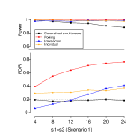
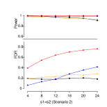
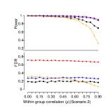
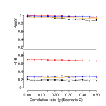
Figure 1: The power and the FDR of generalized simultaneous, pooling, intersection and individual methods for continuous data setting when varying $s_{1}=s_{2}$ in scenario 1 (row1, left) and scenario 2 (row1, right), within-group correlations $\rho_{1}=\rho_{2}$ (row 2, left) and correlation ratio $\gamma_{1}=\gamma_{2}$ (row2, right) for $s_{1}=s_{2}=16$ case in Scenario 2.

Figure 2 compares the power and the FDR on binary and mixed data settings for three cases (1. $s_{1}=s_{2}=0$; 2. $s_{1}=s_{2}\neq 0$; 3. $s_{1}=0,s_{2}\neq 0$) among three methods: GS knockoffs, pooling, and intersection. The results are consistent with continuous data settings. Our GS knockoff method controls FDR all the time in those settings. The intersection method controls FDR but has less power than our method there are only simultaneous signals ($s_{1}=s_{2}=0$). The pooling method always has the highest power among the three methods but it cannot control FDR for two samples with a large number of true signals.

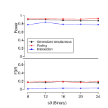
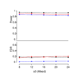
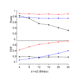
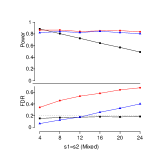
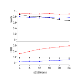
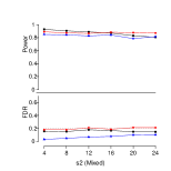
Figure 2: The power and the FDR of generalized simultaneous, pooling and intersection methods when varying $s_{0}$ (row 1), $s_{1}=s_{2}$ (row 2), and $s_{2}$ (row 3) for Scenario 1 (same strengths) under binary (left) and mixed (right) data settings.

The simulation results are consistent with our theoretical expectations. In terms of FDR, the proposed GS knockoff method controls FDR across all designed settings while the other methods fail. The pooling method can control FDR only when there are only simultaneous signals exist ($s_{1}=s_{2}=0$). The intersection method controls FDR when only simultaneous signals exist($s_{1}=s_{2}=0$) and non-mutual signals exist in one group ($s_{1}=0,s_{2}\neq 0$). In terms of power, the GS knockoff method has good power, which is similar to the pooing method and is slightly higher than the intersection method when only simultaneous signals exist($s_{1}=s_{2}=0$). When non-mutual signals exist in one group ($s_{1}=0,s_{2}\neq 0$), GS knockoff, pooling, and intersection methods have similar power. And the performance between scenario 1 (same strengths) and scenario 2 (different signal strengths) of our method are very similar, with all the FDR being controlled.

More results for both Scenario 1 and 2 in three data settings: continuous, binary, and mixed are shown in Appendix E.

6 The N3C data analysis

In this section, we demonstrate the application of our proposed GS knockoff method to the N3C data for the selection of risk factors of long COVID from a collection of baseline patient demographic, comorbidity and medication information. Our data is from the N3C Knowledge Store Shared Project. The N3C enclave consists of EHR data for over 6 million patients with confirmed COVID infection. It also contains high-dimensional patient demographic, comorbidity, medication, social economical information. As of January 25, 2023, there are over 77 data-contributing sites to the N3C data enclave. In this application, to avoid demanding computing time and memory, we construct a toy example with a moderate sample size and a moderate number of candidate features to demonstrate our method. The cohort is constructed by a matched case-control sampling of patients with confirmed COVID infection from two data partners ($n_{1}=12982$ in site 124 and $n_{2}=3100$ in site 967). Information on whether the patient has developed long COVID after the acute COVID has been recorded in the two data sites differently. In data site 124, a binary long COVID U9.09 diagnosis is provided as the long COVID outcome, whereas in site 967, a binary long COVID clinical visit index is recorded as the long COVID outcome. These two long COVID indicators are highly related but not the same. A list of patient baseline information has been extracted as (group level) candidate risk factors ($M=43$). For some of the candidate variables, the data from the two sites are recorded differently (for example, the ”race-ethnicity” variable has different numbers of levels). Our goal for this analysis is to identify mutual risk factors for these two outcomes. Details on the cohort construction and candidate risk factors can be found in Appendix F.

We create dummy variables for the categorical variables and use the GS knockoff method with the second order method for the knockoff construction in Step 1, the group knockoff+ filter with the $\textnormal{FDR}_{\textnormal{group}}$ controlled at 0.2. We also compare the result with the selection using the group knockoff filter.

Using the group knockoff+ filter, 16 risk factors are selected: sex, age at covid, race, dementia, obesity, coronary-artery disease, systemic corticosteroids, depression, metastatic solid tumor cancers, chronic lung disease, myocardial infarction, cardiomyopathies, hypertension, negative antibody, number of covid vaccine doses and covid associated emergency department visit. Using the group knockoff filter, 17 risk factors are selected, including 16 risk factors the same as risk factors selected using group knockoff+ and sickle-cell disease.

7 Discussion

In this paper, we present a novel GS knockoff method, which allows us to control FDR in testing the union null hypotheses on conditional associations between group-level candidate features and outcomes. Like other knockoff-based methods, the GS knockoffs can work with very general conditional model settings and covariate structures within the individual datasets, assuming the independence between the datasets. This method allows us to collectively use information from datasets with different dependencies of $Y|\mathbf{X}$, different outcomes $Y$, and heterogeneous $\mathbf{X}$ structures, allowing for different data types and different group sizes across multiple datasets. The FDR control guarantee is exact for finite sample settings.

This method has broad applications beyond the N3C long COVID real data example. For example, in EHR data from multiple data centers, some covariates are recorded differently among the centers (for example, some centers record the body mass index (BMI) as a continuous variable, but others as an ordinal categorical variable); some groups of variables are of different group sizes (for example, for a solid organ transplant, different centers report different lists of organs); and the demographic distributions are different across the data sources. The GS knockoff method can be used to identify mutual signals with more reliable associations. This method also requires very limited information (only the test statistics) to be shared among the data centers, which benefits data collaboration under privacy protections.

Under the GS knockoff framework, both the Fixed-X and Model-X knockoff approaches can be used for the individual datasets. The framework is compatible with all the existing knockoff and group knockoff construction methods. In this work, we develop a list of group knockoff construction methods to work with both the Fixed-X and Model-X knockoff approaches.

Appendix A Technical Lemmas

Lemma A.1.

For the $\widetilde{X}$ generated from Algorithm 1, it satisfies the group model-X knockoff requirements.

Proof.

Since the generation is without looking at $Y$, so the second condition holds automatically. Here we just need to verify the first condition. Since $(\mathbf{X}_{G_{1}},\widetilde{\mathbf{X}}_{G_{1}})|\mathbf{X}_{-G_{1}}\stackrel{{\scriptstyle\mathclap{\mbox{d}}}}{{=}}(\widetilde{\mathbf{X}}_{G_{1}},\mathbf{X}_{G_{1}})|\mathbf{X}_{-G_{1}}$, we have $(\mathbf{X},\widetilde{\mathbf{X}}_{G_{1}})\stackrel{{\scriptstyle\mathclap{\mbox{d}}}}{{=}}(\mathbf{X},\widetilde{\mathbf{X}}_{G_{1}})_{GSwap(1)}$. Now, we use proof by induction similar as Candes et al. (2018) to show that $(\mathbf{X},\widetilde{X}_{G_{1}},\dots,\widetilde{X}_{m})\stackrel{{\scriptstyle\mathclap{\mbox{d}}}}{{=}}(\mathbf{X},\widetilde{X}_{G_{1}},\widetilde{X}_{G_{m}})_{GSwap(S)}$ for any $S\in[m]$ after $m$ steps. Since the swap of multiple groups can be performed in multiple steps with a swap of one group at a time, we just need to prove the setting for $S=\{j\}$ for $j\in[m]$. Notice the measure for the joint distribution can be written as

$$dP(\mathbf{X},\widetilde{\mathbf{X}}_{\cup_{j=1}^{m}G_{j}}) = dP(\mathbf{X},\widetilde{\mathbf{X}}_{\cup_{j=1}^{m-1}G_{j}})\frac{dP(\widetilde{\mathbf{X}}_{G_{j}},\mathbf{X},\widetilde{\mathbf{X}}_{\cup_{j=1}^{m-1}G_{j}})}{dP(\mathbf{X},\widetilde{\mathbf{X}}_{\cup_{j=1}^{m-1}G_{j}})}$$

$$= dP(\mathbf{X}_{-G_{j}},\mathbf{X}_{-G_{j}},\widetilde{\mathbf{X}}_{\cup_{j=1}^{m-1}G_{j}})\frac{dP(\mathbf{X}_{-G_{j}},\widetilde{\mathbf{X}}_{G_{j}},\widetilde{\mathbf{X}}_{\cup_{j=1}^{m-1}G_{j}}))}{\int dP(\mathbf{X}_{-G_{j}},du,\widetilde{\mathbf{X}}_{\cup_{j=1}^{m-1}G_{j}})}$$

Changing $\mathbf{X}_{G_{j}}$ and $\widetilde{X}_{G_{j}}$ will lead to the same numerator and when $j<m$, by induction, the denominator does not change and when $j=m$, the denominator does not depend on $\mathbf{X}_{G_{j}}$ and $\tilde{X}_{G_{j}}$, so the group exchangeability holds.

Now after the $M$ steps, we get the knockoff that satisfies condition 1 of the group model-X knockoff construction. ∎

Lemma A.2.

For the $\widetilde{X}$ generated from the sequential group knockoff, it satisfies the group model-X knockoff requirements when the model is correctly specified and the true parameters are used.

Proof.

When the model is correctly specified and true parameters are used, we have

$$\widetilde{\mathbf{X}}_{G_{m}}^{con}|\mathbf{X}_{-G_{m}},\widetilde{\mathbf{X}}_{\cup_{j=1}^{m-1}G_{j}}\stackrel{{\scriptstyle\mathclap{\mbox{d}}}}{{=}}\mathbf{X}_{G_{m}}^{con}|\mathbf{X}_{-G_{m}},\widetilde{\mathbf{X}}_{\cup_{j=1}^{m-1}G_{j}}$$

$$\widetilde{\mathbf{X}}_{G_{m}}^{cat}|\widetilde{\mathbf{X}}_{G_{m}}^{cat},\mathbf{X}_{-G_{m}},\widetilde{\mathbf{X}}_{\cup_{j=1}^{m-1}G_{j}}\stackrel{{\scriptstyle\mathclap{\mbox{d}}}}{{=}}\mathbf{X}_{G_{m}}^{con}|\widetilde{\mathbf{X}}_{G_{m}}^{cat},\mathbf{X}_{-G_{m}},\widetilde{\mathbf{X}}_{\cup_{j=1}^{m-1}G_{j}}$$

which together implies

$$\widetilde{\mathbf{X}}_{G_{m}}|\mathbf{X}_{-G_{m}},\widetilde{\mathbf{X}}_{\cup_{j=1}^{m-1}G_{j}}\stackrel{{\scriptstyle\mathclap{\mbox{d}}}}{{=}}\mathbf{X}_{G_{m}}|\mathbf{X}_{-G_{m}},\widetilde{\mathbf{X}}_{\cup_{j=1}^{m-1}G_{j}},$$

and this follows the general group model-X knockoff generation procedure. So applying Lemma A.1 finishes the proof. ∎

The GS knockoff procedure robustness against the misspecification of the distribution of $\mathbf{X}$. In real applications, when we have additional samples of $\mathbf{X}$ (for estimating the distribution of $\mathbf{X}$), we will be able to approximate the $\mathbf{X}$ distribution well. Theorem 2 of Dai & Zheng (2021) can be easily extended to show an FDR upper bound result for GS knockoffs.

Lemma A.3.

Let $\mathbf{W}=f([\mathbf{Z}^{1},\widetilde{\mathbf{Z}}^{1}],\cdots,[\mathbf{Z}^{K},\widetilde{\mathbf{Z}}^{K}])$ where $f$ is an OSFF. Let $\epsilon\in\{\pm 1\}^{M}$ be a sign sequence independent of $\mathbf{W}$, with $\epsilon_{j}=+1$ for all $j\in\mathcal{S}$ and $\epsilon_{j}\sim\{\pm 1\}$ for all $j\in\mathcal{H}$. Then $(W_{1},\cdots,W_{M})\stackrel{{\scriptstyle\mathclap{\mbox{d}}}}{{=}}(W_{1}\cdot\epsilon_{1},\cdots,W_{M}\cdot\epsilon_{M})$.

Proof.

For any $S\subseteq\mathcal{H}$, we can write it as the union of $K$ subsets $S=\cup_{k=1}^{K}S_{k}$, where $S_{k}\subseteq\mathcal{H}_{k}$ for $k=1,\cdots,K$, and $S_{k1}\cap S_{k2}=\emptyset$ for all $k_{1}\neq k_{2}$. In particular, we can let $S_{k}=S\cap\mathcal{H}_{k}\cap(\cup_{j=1}^{k-1}\mathcal{H}_{j})^{c}$. Since $S_{k}\subseteq\mathcal{H}_{k}$, for $k\in[K]$, any statistics $[\mathbf{Z}^{k},\widetilde{\mathbf{Z}}^{k}]=w([\mathbf{X}^{k},\widetilde{\mathbf{X}}^{k}],\mathbf{Y}^{k})$, by the construction of knockoffs, satisfy $[\mathbf{Z}^{k},\widetilde{\mathbf{Z}}^{k}]\stackrel{{\scriptstyle\mathclap{\mbox{d}}}}{{=}}[\mathbf{Z}^{k},\widetilde{\mathbf{Z}}^{k}]_{\textnormal{Swap}(S_{k})}$. By the mutually independence between $[Z^{1},\widetilde{Z}^{1}],\cdots,[Z^{K},\widetilde{Z}^{K}]$, we have

$$f\left([\mathbf{Z}^{1},\widetilde{\mathbf{Z}}^{1}]_{\textnormal{Swap}(S_{1})},\cdots,[\mathbf{Z}^{K},\widetilde{\mathbf{Z}}^{K}]_{\textnormal{Swap}(S_{K})}\right)\stackrel{{\scriptstyle\mathclap{\mbox{d}}}}{{=}}f\left([\mathbf{Z}^{1},\widetilde{\mathbf{Z}}^{1}],\cdots,[\mathbf{Z}^{K},\widetilde{\mathbf{Z}}^{K}]\right).$$

Using the definition of the OSFF, we have

$$f\left([\mathbf{Z}^{1},\widetilde{\mathbf{Z}}^{1}]_{\textnormal{Swap}(S_{1})},[\mathbf{Z}^{2},\widetilde{\mathbf{Z}}^{2}]_{\textnormal{Swap}(S_{2})},\cdots,[\mathbf{Z}^{K},\widetilde{\mathbf{Z}}^{K}]_{\textnormal{Swap}(S_{K})}\right)$$

$$= f\left([\mathbf{Z}^{1},\widetilde{\mathbf{Z}}^{1}],[\mathbf{Z}^{2},\widetilde{\mathbf{Z}}^{2}]_{\textnormal{Swap}(S_{2})},\cdots,[\mathbf{Z}^{K},\widetilde{\mathbf{Z}}^{K}]_{\textnormal{Swap}(S_{K})}\right)\odot\epsilon(S_{1})$$

$$= \cdots$$

$$= f\left([\mathbf{Z}^{1},\widetilde{\mathbf{Z}}^{1}],[\mathbf{Z}^{2},\widetilde{\mathbf{Z}}^{2}],\cdots,[\mathbf{Z}^{K},\widetilde{\mathbf{Z}}^{K}]\right)\odot_{k=1}^{K}\epsilon(S_{k})$$

$$= f\left([\mathbf{Z}^{1},\widetilde{\mathbf{Z}}^{1}],[\mathbf{Z}^{2},\widetilde{\mathbf{Z}}^{2}],\cdots,[\mathbf{Z}^{K},\widetilde{\mathbf{Z}}^{K}]\right)\odot\epsilon(S).$$

So we obtain

$$\mathbf{W}=f\left([\mathbf{Z}^{1},\widetilde{\mathbf{Z}}^{1}],\cdots,[\mathbf{Z}^{K},\widetilde{\mathbf{Z}}^{K}]\right)\stackrel{{\scriptstyle\mathclap{\mbox{d}}}}{{=}}f\left([\mathbf{Z}^{1},\widetilde{\mathbf{Z}}^{1}],\cdots,[\mathbf{Z}^{K},\widetilde{\mathbf{Z}}^{K}]\right)\odot\epsilon(S)=\mathbf{W}\odot\epsilon(S).$$

for any $S\subseteq\mathcal{H}$. Therefore, by choosing $S$ as the set $\{j:\epsilon_{j}=-1\}$, we have

$$(W_{1},\cdots,W_{M})\stackrel{{\scriptstyle\mathclap{\mbox{d}}}}{{=}}(W_{1}\cdot\epsilon_{1},\cdots,W_{M}\cdot\epsilon_{M}).$$

and thus we finish the proof of the lemma. ∎

Lemma A.4.

For $k=m,m-1,\cdots,1,0$, put $V^{+}(k)=\#\{j:1\leq j\leq k,p_{j}\leq 1/2,j\in\mathcal{H}\}$ and $V^{-}(k)=\#\{j:1\leq j\leq k,p_{j}>1/2,j\in\mathcal{H}\}$ with the convention that $V^{\pm}(0)=0$. Let $\mathcal{F}_{k}$ be the filtration defined by knowing all the non-null $p$-values, as well as $V^{\pm}(k^{\prime})$ for all $k^{\prime}\geq k$. Then the process $M(k)=\frac{V^{+}(k)}{1+V^{-}(k)}$ is a super-martingale running backward in time with respect to $\mathcal{F}_{k}$. For any fixed $q$, $\widehat{k}=\widehat{k}_{+}$ or $\widehat{k}=\widehat{k}_{0}$ as defined in the proof of theorem 1 are stopping times, and as consequences

$$\mathbb{E}\left[{\frac{\#\{j\leq\widehat{k}:p_{j}\leq 1/2,j\in\mathcal{H}\}}{1+\#\{j\leq\widehat{k}:p_{j}>1/2,j\in\mathcal{H}\}}}\right]\leq 1$$

Proof.

The filtration $\mathcal{F}_{k}$ contains the information of whether $k$ is null and non-null process is known exactly. If $k$ is non-null, then $M(k-1)=M(k)$ and if $k$ is null, we have

$$M(k-1)=\frac{V^{+}(k)-\mathbbm{1}_{p_{k}\leq 1/2}}{1+V^{-}(k)-(1-\mathbbm{1}_{p_{k}\leq 1/2})}=\frac{V^{+}(k)-\mathbbm{1}_{p_{k}\leq 1/2}}{\left(V^{-}(k)+\mathbbm{1}_{p_{k}\leq 1/2}\right)\vee 1}$$

Given that nulls are i.i.d., we have

$$\mathbb{P}\left\{{\mathbbm{1}_{p_{k}\leq 1/2}|\mathcal{F}_{k}}\right\}=\frac{V^{+}(k)}{\left(V^{+}(k)+V^{-}(k)\right)}.$$

So when $k$ is null, we have

$$\mathbb{E}\left[{M(k-1)|\mathcal{F}_{k}}\right] = \frac{1}{V^{+}(k)+V^{-}(k)}\left[V^{+}(k)\frac{V^{+}(k)-1}{V^{-}(k)+1}+V^{-}(k)\frac{V^{+}(k)}{V^{-}(k)\vee 1}\right]$$

$$= \frac{V^{+}(k)}{1+V^{-}(k)}\mathbbm{1}_{V^{-}(k)>0}+(V^{+}(k)-1)\mathbbm{1}_{V^{-}(k)=0}$$

$$\leq M(k)$$

This finishes the proof of super-martingale property. $\widehat{k}$ is a stopping time with respect to $\{\mathcal{F}_{k}\}$ since $\{\widehat{k}\geq k\}\in\mathcal{F}_{k}$. So we have $\mathbb{E}\left[{M(\widehat{k})}\right]\leq\mathbb{E}\left[{M(m)}\right]=\mathbb{E}\left[{\frac{\#\{j:p_{j}\leq 1/2,j\in\mathcal{H}\}}{1+\#\{j:p_{j}>1/2,j\in\mathcal{H}\}}}\right]$.

Let $X=\#\{j:p_{j}\leq 1/2,j\in\mathcal{H}\}$, given that $p_{j}\geq Unif[0,1]$ independently for all nulls, we have $X\leq_{d}Binomial(N,1/2)$. Let $Y\sim Binomial(N,1/2)$ where $N$ is the total number of nulls. Given that $f(x)=\frac{x}{1+N-x}$ is non-decreasing, we have

$$\mathbb{E}\left[{\frac{X}{1+N-X}}\right] \leq \mathbb{E}\left[{\frac{Y}{1+N-Y}}\right]$$

$$= \sum_{i=1}^{N}(1/2)^{N}\frac{N!}{i!(N-i)!}\frac{i}{1+N-i}$$

$$= \sum_{i=1}^{N}\mathbb{P}\left\{{Y=i-1}\right\}$$

$$\leq 1.$$

∎

Appendix B Proof of the main theorem (Theorem 4.1)

The proof of Theorem 4.1 follows the proof idea in Barber & Candès (2015). Let $m=\#\{j:W_{j}\neq 0\}$ and assume without loss of generality that $|W_{1}|\geq|W_{2}|\geq\cdots\geq|W_{m}|>0$. Define p-values $p_{j}=1$ if $W_{j}<0$ and $p_{j}=1/2$ if $W_{j}>0$, then Lemma 1 implies that null $p$-values are $i.i.d.$ with $p_{j}\geq\text{Unif}[0,1]$ and are independent from nonnulls.

We first show the result for the knockoff+ threshold. Define $V=\#\{j\leq\widehat{k}_{+}:p_{j}\leq 1/2,j\in\mathcal{H}\}$ and $R=\#\{j\leq\widehat{k}_{+}:p_{j}\leq 1/2\}$ where $\widehat{k}_{+}$ satisfy that $|W_{\widehat{k}_{+}}|=\tau_{+}$ where $\tau_{+}$ is defined in theorem 1, we have

$$\mathbb{E}\left[{\frac{V}{R\vee 1}}\right]=\mathbb{E}\left[{\frac{V}{R\vee 1}\mathbbm{1}_{\widehat{k}_{+}>0}}\right]$$

$$= \mathbb{E}\left[{\frac{\#\{j\leq\widehat{k}_{+}:p_{j}\leq 1/2,j\in\mathcal{H}\}}{1+\#\{j\leq\widehat{k}_{+}:p_{j}>1/2,j\in\mathcal{H}\}}\left(\frac{1+\#\{j\leq\widehat{k}_{+}:p_{j}>1/2,j\in\mathcal{H}\}}{\#\{j\leq\widehat{k}_{+}:p_{j}\leq 1/2\}\vee 1}\right)\mathbbm{1}_{\widehat{k}_{+}>0}}\right]$$

$$\leq \mathbb{E}\left[{\frac{\#\{j\leq\widehat{k}_{+}:p_{j}\leq 1/2,j\in\mathcal{H}\}}{1+\#\{j\leq\widehat{k}_{+}:p_{j}>1/2,j\in\mathcal{H}\}}}\right]q\leq q,$$

where the first inequality holds by the definition of $\widehat{k}_{+}$ and the second inequality holds by Lemma A.4.

Similarly, for the knockoff threshold, we have $V=\#\{j\leq\widehat{k}_{0}:p_{j}\leq 1/2,j\in\mathcal{H}\}$ and $R=\#\{j\leq\widehat{k}_{0}:p_{j}\leq 1/2\}$ where $\widehat{k}_{0}$ satisfies that $|W_{\widehat{k}_{0}}|=\tau$ where $\tau$ is defined as in theorem 1, then

$$\mathbb{E}\left[{\frac{V}{R+q^{-1}}}\right]$$

$$= \mathbb{E}\left[{\frac{\#\{j\leq\widehat{k}_{0}:p_{j}\leq 1/2,j\in\mathcal{H}\}}{1+\#\{j\leq\widehat{k}_{0}:p_{j}>1/2,j\in\mathcal{H}\}}\left(\frac{1+\#\{j\leq\widehat{k}_{0}:p_{j}>1/2,j\in\mathcal{H}\}}{\#\{j\leq\widehat{k}_{0}:p_{j}\leq 1/2\}+q^{-1}}\right)\mathbbm{1}_{\widehat{k}_{0}>0}}\right]$$

$$\leq \mathbb{E}\left[{\frac{\#\{j\leq\widehat{k}_{0}:p_{j}\leq 1/2,j\in\mathcal{H}\}}{1+\#\{j\leq\widehat{k}_{0}:p_{j}>1/2,j\in\mathcal{H}\}}}\right]q\leq q,$$

where the first inequality holds by the definition of $\widehat{k}_{0}$ and the second inequality holds by Lemma A.4.

Appendix C Proof of the corollary

Proof.

First, we noticed that for $m\in S$,

$$W_{m} = f([\mathbf{Z}^{1},\widetilde{\mathbf{Z}}^{1}],\cdots,[\mathbf{Z}^{k},\widetilde{\mathbf{Z}}^{k}]_{\textnormal{Swap}(S)},\cdots,[\mathbf{Z}^{K},\widetilde{\mathbf{Z}}^{K}])_{m}$$

$$= \prod_{j\in[K]\backslash k}(Z^{j}_{m}-\widetilde{Z}^{j}_{m})(\widetilde{Z}_{m}^{k}-Z_{m}^{k})$$

$$= -\prod_{j\in[K]}(Z^{j}_{m}-\widetilde{Z}^{j}_{m})$$

$$= -f([\mathbf{Z}^{1},\widetilde{\mathbf{Z}}^{1}],\cdots,[\mathbf{Z}^{K},\widetilde{\mathbf{Z}}^{K}])_{m},$$

and for $m\notin S$

$$W_{m} = f([\mathbf{Z}^{1},\widetilde{\mathbf{Z}}^{1}],\cdots,[\mathbf{Z}^{k},\widetilde{\mathbf{Z}}^{k}]_{\textnormal{Swap}(S)},\cdots,[\mathbf{Z}^{K},\widetilde{\mathbf{Z}}^{K}])_{m}$$

$$= \prod_{j\in[K]\backslash k}(Z^{j}_{m}-\widetilde{Z}^{j}_{m})(Z_{m}^{k}-\widetilde{Z}_{m}^{k})$$

$$= \prod_{j\in[K]}(Z^{j}_{m}-\widetilde{Z}^{j}_{m})$$

$$= f([\mathbf{Z}^{1},\widetilde{\mathbf{Z}}^{1}],\cdots,[\mathbf{Z}^{K},\widetilde{\mathbf{Z}}^{K}])_{m},$$

So we have

$$W = f([\mathbf{Z}^{1},\widetilde{\mathbf{Z}}^{1}],\cdots,[\mathbf{Z}^{k},\widetilde{\mathbf{Z}}^{k}]_{\textnormal{Swap}(S)},\cdots,[\mathbf{Z}^{K},\widetilde{\mathbf{Z}}^{K}])$$

$$= f([\mathbf{Z}^{1},\widetilde{\mathbf{Z}}^{1}],\cdots,[\mathbf{Z}^{k},\widetilde{\mathbf{Z}}^{k}],\cdots,[\mathbf{Z}^{K},\widetilde{\mathbf{Z}}^{K}])\odot\epsilon(S)$$

and thus the OSFF assumption is satisfied.

When Model-X group knockoff construction is used, we notice that based on the construction of group Model-X knockoff, we have $[\mathbf{X}^{k}\widetilde{\mathbf{X}}^{k}]\stackrel{{\scriptstyle\mathclap{\mbox{d}}}}{{=}}[\mathbf{X}^{k}\widetilde{\mathbf{X}}^{k}]_{GSwap(S)}$, $\widetilde{\mathbf{X}}^{k}\perp\!\!\!\perp Y^{k}|\mathbf{X}^{k}$. For any $S\subseteq\mathcal{H}$, we have $[\mathbf{X}^{k},\widetilde{\mathbf{X}}^{k}]|Y^{k}\stackrel{{\scriptstyle\mathclap{\mbox{d}}}}{{=}}[\mathbf{X}^{k},\widetilde{\mathbf{X}}^{k}]_{GSwap(S)}|Y^{k}$. By the definition of knockoff-compatible statistics, we have

$$[\mathbf{Z}^{k},\widetilde{\mathbf{Z}}^{k}]_{Swap(S)}=t([\mathbf{X}^{k},\widetilde{\mathbf{X}}^{k}]_{GSwap(S)},Y^{k})$$

$$=^{d} t([\mathbf{X}^{k},\widetilde{\mathbf{X}}^{k}],Y^{k})$$

$$= [\mathbf{Z}^{k},\widetilde{\mathbf{Z}}^{k}]$$

for any $S\subseteq\mathcal{H}$. When fixed group knockoff construction is used, by the definition of knockoff compatible statistics and sufficiency requirement, we have

$$[\mathbf{Z}^{k},\widetilde{\mathbf{Z}}^{k}]_{Swap(S)}=t([\mathbf{X}^{k},\widetilde{\mathbf{X}}^{k}]^{\top}_{GSwap(S)}[\mathbf{X}^{k},\widetilde{\mathbf{X}}^{k}]_{GSwap(S)},[\mathbf{X}^{k},\widetilde{\mathbf{X}}^{k}]_{GSwap(S)}^{\top}Y^{k})$$

$$=^{d} t([\mathbf{X}^{k},\widetilde{\mathbf{X}}^{k}]^{\top}[\mathbf{X}^{k},\widetilde{\mathbf{X}}^{k}],[\mathbf{X}^{k},\widetilde{\mathbf{X}}^{k}]^{\top}Y^{k})$$

$$= [\mathbf{Z}^{k},\widetilde{\mathbf{Z}}^{k}].$$

Applying Theorem 4.1, we obtain the conclusion for this corollary. ∎

Appendix D Additional simulation details

D.1 Data Generation

Continuous.

We set both experiments to have the same sample size $n_{k}=1000$ and the same number of groups of features $M=80$. We have the 5 features per group for each group (i.e, $G_{km}=\{5m-4,\cdots,5m\}$ for $k\in[K],m\in[M]$ and $p_{1}=p_{2}=400$ features in total for each experiment). We simulate independent $X^{k}$s for $k\in[K]$ such that

$$\mathbf{X}_{i}^{k}\sim\mathcal{N}(\mathbf{0},\Sigma^{k})~{}\text{for}~{}i\in[n_{k}],$$

where $\Sigma^{k}\in\mathbb{R}^{p_{k}\times p_{k}}$ with diagonal elements $\Sigma_{jj}^{k}=1$ for $j\in[p_{k}]$, within-group correlations $\Sigma_{ji}^{k}=\rho_{k}$ for $i\neq j$ in the same group (i.e., $\{i,j\}\subset G_{km}$ for some $m\in[M]$) and between-group correlations $\Sigma_{ji}^{k}=\gamma_{k}\rho_{k}$ for $j\neq i$ in different groups (i.e., There is no $m\in[M]$ such that $\{i,j\}\subset G_{km}$).

Next, we generate the coefficients $\beta^{1},\cdots,\beta^{K}$ for the $K$ experiments. We denote $s_{0}$ as the number of groups of simultaneous signals among the $K$ datasets, $s_{k}$ as the number of groups of signals specifically for the $k$-th datasets. We consider two scenarios: (1) both directions and strengths of the mutual signals are the same among the $K$ datasets, and (2) only the directions of the mutual signals are the same but the signal strengths are different among the K datasets. For both datasets, the signal strengths within each group $m\in[M]$ are identical.

For Scenario 1, we sample $\omega_{j}\in\mathbb{R}^{s_{j}},j\in\{0,1,2\}$, with their elements $\omega_{ji}\sim\textnormal{Uniform}[0,A]$ independent for $i=1,\cdots,s_{j}$. Then we sample $\epsilon\in\{-1,1\}^{M}$ where $\epsilon_{m}$ are independently sampled from Rademacher distribution for $l=1,\cdots,M$. With $K=2$, the coefficients $\beta^{1},\beta^{2}$ are determined by:

$$\beta^{1} = ((\omega_{0}^{\top},\omega_{1}^{\top},\mathbf{0}_{M-s_{0}-s_{1}}^{\top})^{\top}\odot\epsilon)\otimes\mathbf{1}_{5}^{\top},$$

$$\beta^{2} = ((\omega_{0}^{\top},\mathbf{0}_{s_{1}}^{\top},\omega_{2}^{\top},\mathbf{0}_{M-s_{0}-s_{1}-s_{2}}^{\top})^{\top}\odot\epsilon)\otimes\mathbf{1}_{5}^{\top},$$

where $\otimes$ is the Kronecker product and $\odot$ is the Hadamard product.

For Scenario 2, we generate $\omega_{0k}\in\mathbb{R}^{s_{0}}$ for $k\in[K]$ independently; i.e., we sample $\omega_{0ki}\sim\textnormal{Uniform}[0,A]$ independently for $k\in[K]$ and $i=1,\cdot,s_{0}$. We generate $\omega_{1}$, $\omega_{2}$, and $\epsilon$ the same way as described in Scenario 1. The coefficients $\beta^{1},\beta^{2}$ are determined by:

$$\beta^{1} = ((\omega_{01}^{\top},\omega_{1}^{\top},\mathbf{0}_{M-s_{0}-s_{1}}^{\top})^{\top}\odot\epsilon)\otimes\mathbf{1}_{5}^{\top}$$

$$\beta^{2} = ((\omega_{02}^{\top},\mathbf{0}_{s_{1}}^{\top},\omega_{2}^{\top},\mathbf{0}_{M-s_{0}-s_{1}-s_{2}}^{\top})^{\top}\odot\epsilon)\otimes\mathbf{1}_{5}^{\top}.$$

Then $Y_{i}^{k}$s are obtained from the following linear model:

$$Y^{k}_{i} = \beta^{k\top}\mathbf{X}^{k}_{i}+\varepsilon^{k}_{i},$$

where $\varepsilon_{i}^{k}\sim\mathcal{N}(0,\sigma_{k}^{2})$ for $k=1,2$, and $i=1,\dots,n_{k}$, $\sigma_{k}$ is the signal noise ratio.

Binary.

Our design matrices $\mathbf{X}^{k}$s are composed by a mixture of $M=80$ categorical and continuous variables. For both data sets, without loss of generality, we set the first 20 features as independent categorical variables with 5 categories (each level with probability 0.2) and generate the other 60 features from a multivariate normal distribution with mean 0 and covariance $\Sigma(\gamma)$, where $\Sigma(\gamma)$ is an auto-correlation matrix with its (i,j)-th element equals to $\gamma^{|i-j|}$. For each categorical variable, we create 4 dummy variables and consider them as a group (i.e. $p_{k}=140$ for $k\in[K]$). For continuous variables, each of them is considered as a group.

Next, we generate the coefficients $\beta^{1},\cdots,\beta^{K}\in\mathbb{R}^{p_{k}}$. We randomly select an index set $S_{0}\subseteq[M]$ with length $|S_{0}|=s_{0}$ to indicate the mutual group-level signals among the $K$ datasets and mutually exclusive sets $S_{k}\subseteq[M]\setminus S_{0},~{}\text{for}~{}k\in K$ with $|S_{k}|=s_{k}$ as the indices for the exclusive signals for the $k$-th dataset. For the random selection, we stratified by the type of variable (categorical vs continuous) to keep the ratio between categorical variables and continuous variables in $S_{0}$, $\dots$, $S_{K}$ to be 1:3. Then we randomly generate the magnitudes and directions of the $\beta$ elements independently in the signal sets.

Let $\bar{\mathbf{X}}^{k}$ denote the expanded design matrix of $\mathbf{X}^{k}$ after replacing each categorical variable with dummy variables. Then we generate $Y^{k}$ from logistic models:

$$Y^{k}_{i}\sim\textnormal{Bernoulli}\left(\frac{\exp(\alpha_{k}+\beta^{k\top}\bar{\mathbf{X}}^{k}_{i})}{1+\exp(\alpha_{k}+\beta^{k\top}\bar{\mathbf{X}}^{k}_{i})}\right),$$

where $k=1,2~{}\text{and}~{}i=1,\cdots,n_{k}$.

Mixed.

We first generate $\mathbf{X}^{k}$s and $\beta^{k}$s the same as the binary case and expand the design matrix to obtain $\bar{\mathbf{X}}^{k}$. Then we generate the latent outcome $\overline{Y}^{k}$s for $k\in[K]$ from the linear models:

$$\overline{Y}^{k}_{i} = \beta^{k\top}\bar{\mathbf{X}}^{k}_{i}+\varepsilon^{k}_{i},$$

where $\varepsilon_{i}^{k}\sim\mathcal{N}(0,\sigma_{k}^{2})$ for $k=1,2$, and $i=1,\dots,n_{k}$, $\sigma_{k}$ is the signal noise ratio. Then we set $Y_{i}^{1}=\overline{Y}_{i}^{1}$ and set a threshold for $\overline{Y}_{i}^{2}$ to construct the binary $Y_{i}^{2}$:

$$Y^{2}_{i}=\mathbbm{1}\{\overline{Y}^{2}_{i}\geq 0\},~{}\text{where}~{}i=1,\cdots,n_{2}.$$

.

D.2 Simulation settings

We conduct simulations to check the effects of sparsity levels $s_{0},s_{1},s_{2}$ and different correlation structures. To be specific, for the continuous case, we set the amplitude of signals $A=0.6$, the within-group correlations $\rho_{k}=0.5,~{}\text{for}~{}k\in[K]$, and the between-group correlations are set to be $\gamma_{k}\rho_{k},~{}\text{for}~{}k\in[K]$, with the default correlation ratio $\gamma_{k}=0.1$. To understand the effects of sparsity levels, within and between group correlations respectively, we vary one of three kinds of parameters (sparsity levels parameters, within-group correlation parameters, and correlation ratio parameters) in each simulation study and fix the other two kinds of parameters.

• Sparsity level parameters: $s_{0},s_{1},s_{2}.$ We fix $\gamma_{k}=0.1$, and $\rho_{k}=0.5$.

  1. Fixing $$s_{1}=s_{2}=0 s_{0}=8,12,16,20,24$$, we vary ;

  2. Fixing $$s_{0}=16 s_{1}=s_{2}=4,8,12,16,20,24$$, we vary ;

  3. Fixing $$s_{0}=16 s_{1}=0 s_{2}=4,8,12,16,20,24$$ and , we vary .

• Within-group correlation parameters: $\rho_{1},\rho_{2}$. We fix $\gamma_{k}=0.1$ and vary within-group correlations $\rho_{1}=\rho_{2}\in\{0,0.1,\dots,0.9\}$ for the following three choice of $s_{0},s_{1},s_{2}$.

  $$s_{0}=16,s_{1}=0,s_{2}=0;$$

  $$s_{0}=16,s_{1}=16,s_{2}=16;$$

  $$s_{0}=16,s_{1}=0,s_{2}=16.$$

• Correlation ratio parameters: $\gamma_{1},\gamma_{2}$. We fix $\rho_{k}=0.5$ and vary correlation ratio $\gamma_{1}=\gamma_{2}\in\{0,0.05,0.1,\dots,0.5\}$ for the following three choice of $s_{0},s_{1},s_{2}$. Then the between-group correlations are calculated as $\rho_{k}\gamma_{k}$.

  $$s_{0}=16,s_{1}=0,s_{2}=0;$$

  $$s_{0}=16,s_{1}=16,s_{2}=16;$$

  $$s_{0}=16,s_{1}=0,s_{2}=16.$$

  For the binary and mixed cases, we only vary the sparsity levels. We fixed the auto-correlation parameter $r_{1}=r_{2}=0.5$, $\alpha_{1}=1,\alpha_{2}=-1$, and vary the sparsity level $s_{0},s_{1},s_{2}.$ as following:

  1. Fixing $$s_{1}=s_{2}=0 s_{0}=8,12,16,20,24$$, we vary ;

  2. Fixing $$s_{0}=16 s_{1}=s_{2}=4,8,12,16,20,24$$, we vary ;

  3. Fixing $$s_{0}=16 s_{1}=0 s_{2}=4,8,12,16,20,24$$ and , we vary .

Appendix E Additional simulation results

In Figure 3 and Figure 4, we show results for continuous setting with Scenario 1 (same strengths) and Scenario 2 (different signal strengths).

For the continuous settings, when only simultaneous signals exist ($s_{1}=s_{2}=0$), three methods GS knockoffs, pooling and intersection control FDR with similar powers for both the Scenario 1(same strengths) and the Scenario 2(different signal strengths) in general. As within group correlation increases, GS knockoff method still has similar power with pooling and is slightly higher than the intersection method ($s_{1}=s_{2}=0$). When there exist non-mutual signals in one group ($s_{1}=0,s_{2}\neq 0$), pooling methods fail to control FDR but the GS knockoffs and intersection still control FDR. When non-mutual signals exist in both groups ($s_{1}=s_{2}\neq 0$), only GS knockoffs can control FDR. The individual method fails to control FDR across all the continuous settings. And the performance between scenario 1(same strengths) and scenario 2(different signal strengths) of our method are very similar, with all the FDR being controlled.

Figure 5 shows the results for binary and mixed data settings with Scenario 2 (different signal strengths). The results are similar to Scenario 1 (same strengths). Our GS knockoffs method controls FDR across all the binary and mixed settings. pooling method can only control FDR when only simultaneous signals exist ($s_{1}=s_{2}=0$) but fail in ($s_{1}=0,s_{2}\neq 0$) and ($s_{1}=s_{2}\neq 0$) cases. The intersection method fails to control FDR when non-mutual signals exist in both groups ($s_{1}=s_{2}\neq 0$). In addition, when only simultaneous signals exist ($s_{1}=s_{2}=0$), our GS knockoffs has similar power with pooling and is slightly higher than intersection. when there exist non-mutual signals in one group ($s_{1}=0,s_{2}\neq 0$), GS knockoffs has similar power with intersection and is slightly lower power than the pooling method.

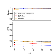
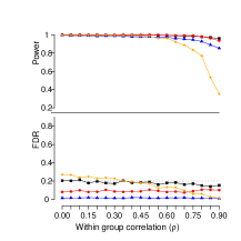
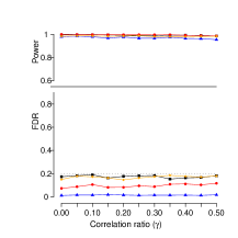
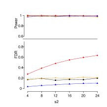
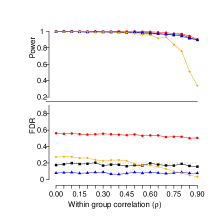
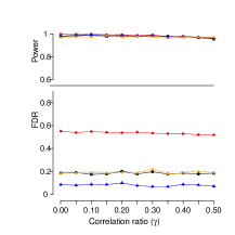
Figure 3: The power and the FDR of generalized simultaneous, pooling, intersection and individual methods when varying sparsity level (left), within-group correlation (middle) and correlation ratio (right) in two cases: 1. $s_{1}=s_{2}=0$ (row 1); 2. $s_{1}=0,s_{2}\neq 0$ (row 2) for Scenario 2 (different signal strengths) under continuous data setting.

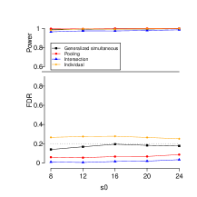
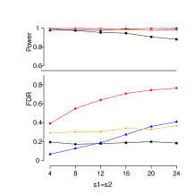
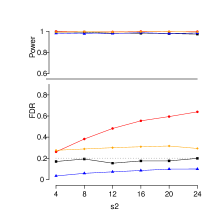
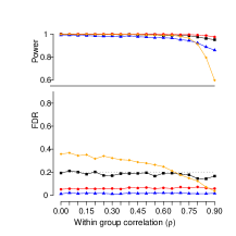
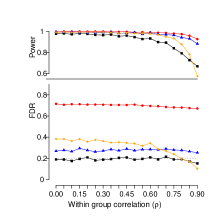
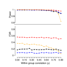
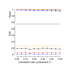
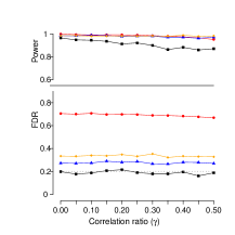
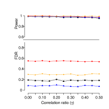
Figure 4: The power and the FDR of generalized simultaneous, pooling, intersection and individual methods when varying sparsity level (row 1), within-group correlation (row 2) and correlation ratio (row 3) in three cases: 1. $s_{1}=s_{2}=0$ (left); 2. $s_{1}=s_{2}\neq 0$ (middle); 3. $s_{1}=0,s_{2}\neq 0$ (right) for Scenario 1 (same strengths) under continuous data setting.

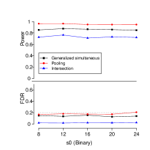
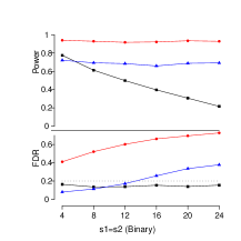
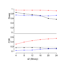
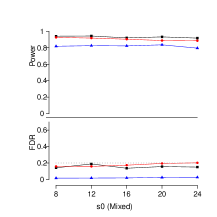
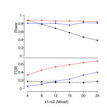
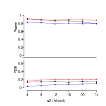
Figure 5: The power and the FDR of generalized simultaneous, pooling and intersection methods when varying $s_{0}$ (left), $s_{1}=s_{2}$ (middle), and $s_{2}$ (right) for Scenario 2 (different signal strengths) under binary (row1) and mixed (row2) data settings.

Appendix F Additional information for real data analysis

The detailed cohort generating inclusion and exclusion steps are illustrated in Figure 6.

There are 43 risk factors included in this analysis: demographic information include sex (”Male”, ”Felmale”), age at covid, race (”Hispanic or Latino Any Race”, ”Others”), indicators include tuberculosis, mild liver disease, moderate severe liver disease, thalassemia, rheumatologic disease, dementia, congestive heart failure, substanceuse disorder, kidney disease, malignant cancer, diabetes complication, cerebrovascular disease, peripheralvascular disease, heart failure, hemiplegia or paraplegia, psychosis, obesity, coronaryartery disease, systemic corticosteroids, depression, metastatic solid tumor cancers, HIV infection, chronic lung disease, peptic ulcer, sickle cell disease, myocardial infarction, diabetes uncomplicated, cardiomyopathies, hypertension, other immunocompromised, negative antibody, pulmonary embolism, tobacco smoker, solid organ or blood stem cell transplant, and some covid related information include number of covid vaccine dose, covid regimen corticosteroids (”Yes” or ”No”), remdesivir usage during covid (”Yes” or ”No”), extracorporeal membrane oxygenation (ECMO) machine usage during covid (”Yes” or ”No”), covid associated hospitalization indicator (”Yes” or ”No”), covid associated emergency department visit (”Yes” or ”No”), and severity type (”Asymptomatic”, ”Mild”, ”Moderate”, ”Severe”). Those indicators indicate patients have been diagnosed with those diseases or symptoms before or on the day they were confirmed to get an acute covid infection (i.e. all the indicators are in two categories: ”Yes”, ”No”). The full data dictionary can be found in https://unite.nih.gov/workspace/report/ri.report.main.report.855e1f58-bf44-4343-9721-8b4c878154fe.

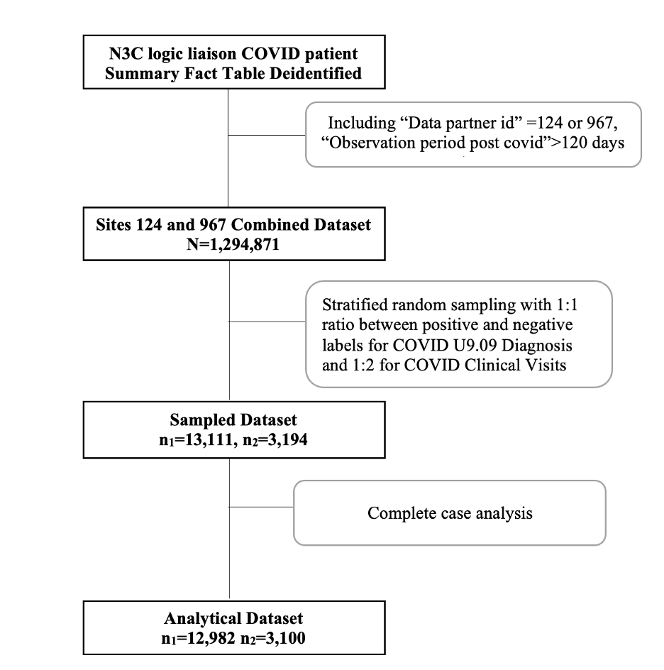
Figure 6: Cohort construction for N3C Knowledge Store Shared Project.

References

- Barber & Candès (2015) Barber, R. F. and Candès, E. J. Controlling the false discovery rate via knockoffs. Ann. Statist., 43(5):2055–2085, 2015. doi: 10.1214/15-AOS1337.
- Barber & Candès (2019) Barber, R. F. and Candès, E. J. A knockoff filter for high-dimensional selective inference. Ann. Statist., 47(5):2504–2537, 2019. doi: 10.1214/18-AOS1755.
- Barber et al. (2020) Barber, R. F., Candès, E. J., and Samworth, R. J. Robust inference with knockoffs. Ann. Statist., 48(3):1409–1431, 2020. doi: 10.1214/19-AOS1852.
- Bates et al. (2020) Bates, S., Candès, E., Janson, L., and Wang, W. Metropolized knockoff sampling. Journal of the American Statistical Association, 2020. doi: 10.1080/01621459.2020.1729163.
- Bogomolov & Heller (2013) Bogomolov, M. and Heller, R. Discovering findings that replicate from a primary study of high dimension to a follow-up study. Journal of the American Statistical Association, 108(504):1480–1492, 2013. doi: 10.1080/01621459.2013.829002.
- Bogomolov & Heller (2018) Bogomolov, M. and Heller, R. Assessing replicability of findings across two studies of multiple features. Biometrika, 105(3):505–516, 2018. ISSN 0006-3444. doi: 10.1093/biomet/asy029.
- Candes et al. (2018) Candes, E., Fan, Y., Janson, L., and Lv, J. Panning for gold:‘model-x’knockoffs for high dimensional controlled variable selection. Journal of the Royal Statistical Society: Series B (Statistical Methodology), 80(3):551–577, 2018.
- Candès et al. (2018) Candès, E., Fan, Y., Janson, L., and Lv, J. Panning for gold: ‘model-x’ knockoffs for high dimensional controlled variable selection. Journal of the Royal Statistical Society: Series B (Statistical Methodology), 80(3):551–577, 2018. doi: https://doi.org/10.1111/rssb.12265.
- Chen et al. (2019) Chen, J., Hou, A., and Hou, T. Y. A prototype knockoff filter for group selection with FDR control. Information and Inference: A Journal of the IMA, 9(2):271–288, 2019. ISSN 2049-8772. doi: 10.1093/imaiai/iaz012.
- Chi (2008) Chi, Z. False discovery rate control with multivariate p -values. Electron. J. Statist., 2:368–411, 2008. doi: 10.1214/07-EJS147.
- Dai & Barber (2016) Dai, R. and Barber, R. The knockoff filter for fdr control in group-sparse and multitask regression. In Balcan, M. F. and Weinberger, K. Q. (eds.), Proceedings of The 33rd International Conference on Machine Learning, volume 48 of Proceedings of Machine Learning Research, pp. 1851–1859, New York, New York, USA, 2016. PMLR.
- Dai & Zheng (2021) Dai, R. and Zheng, C. Multiple testing for composite null with fdr control guarantee. arXiv preprint arXiv:2106.12719, 2021.
- Dai et al. (2022) Dai, X., Lyu, X., and Li, L. Kernel knockoffs selection for nonparametric additive models. Journal of the American Statistical Association, 0(0):1–13, 2022. doi: 10.1080/01621459.2022.2039671. URL https://doi.org/10.1080/01621459.2022.2039671.
- Haendel et al. (2020) Haendel, M. A., Chute, C. G., Bennett, T. D., Eichmann, D. A., Guinney, J., Kibbe, W. A., Payne, P. R. O., Pfaff, E. R., Robinson, P. N., Saltz, J. H., Spratt, H., Suver, C., Wilbanks, J., Wilcox, A. B., Williams, A. E., Wu, C., Blacketer, C., Bradford, R. L., Cimino, J. J., Clark, M., Colmenares, E. W., Francis, P. A., Gabriel, D., Graves, A., Hemadri, R., Hong, S. S., Hripscak, G., Jiao, D., Klann, J. G., Kostka, K., Lee, A. M., Lehmann, H. P., Lingrey, L., Miller, R. T., Morris, M., Murphy, S. N., Natarajan, K., Palchuk, M. B., Sheikh, U., Solbrig, H., Visweswaran, S., Walden, A., Walters, K. M., Weber, G. M., Zhang, X. T., Zhu, R. L., Amor, B., Girvin, A. T., Manna, A., Qureshi, N., Kurilla, M. G., Michael, S. G., Portilla, L. M., Rutter, J. L., Austin, C. P., Gersing, K. R., and the N3C Consortium. The National COVID Cohort Collaborative (N3C): Rationale, design, infrastructure, and deployment. Journal of the American Medical Informatics Association, 28(3):427–443, 08 2020. ISSN 1527-974X. doi: 10.1093/jamia/ocaa196. URL https://doi.org/10.1093/jamia/ocaa196.
- Heller & Yekutieli (2014) Heller, R. and Yekutieli, D. Replicability analysis for genome-wide association studies. Ann. Appl. Stat., 8(1):481–498, 2014. doi: 10.1214/13-AOAS697.
- Heller et al. (2014) Heller, R., Bogomolov, M., and Benjamini, Y. Deciding whether follow-up studies have replicated findings in a preliminary large-scale omics study. Proceedings of the National Academy of Sciences, 111(46):16262–16267, 2014. ISSN 0027-8424. doi: 10.1073/pnas.1314814111.
- Huang & Janson (2020) Huang, D. and Janson, L. Relaxing the assumptions of knockoffs by conditioning. Ann. Statist., 48(5):3021–3042, 2020. doi: 10.1214/19-AOS1920.
- Kormaksson et al. (2021) Kormaksson, M., Kelly, L. J., Zhu, X., Haemmerle, S., Pricop, L., and Ohlssen, D. Sequential knockoffs for continuous and categorical predictors: With application to a large psoriatic arthritis clinical trial pool. Statistics in Medicine, 40(14):3313–3328, 2021. doi: https://doi.org/10.1002/sim.8955. URL https://onlinelibrary.wiley.com/doi/abs/10.1002/sim.8955.
- Langley (2000) Langley, P. Crafting papers on machine learning. In Langley, P. (ed.), Proceedings of the 17th International Conference on Machine Learning (ICML 2000), pp. 1207–1216, Stanford, CA, 2000. Morgan Kaufmann.
- Liu & Zheng (2019) Liu, Y. and Zheng, C. Deep latent variable models for generating knockoffs. Stat, 8(1):e260, 2019. doi: https://doi.org/10.1002/sta4.260. e260 sta4.260.
- Montani et al. (2022) Montani, D., Savale, L., Noel, N., Meyrignac, O., Colle, R., Gasnier, M., Corruble, E., Beurnier, A., Jutant, E.-M., Pham, T., Lecoq, A.-L., Papon, J.-F., Figueiredo, S., Harrois, A., Humbert, M., and Monnet, X. Post-acute covid-19 syndrome. European Respiratory Review, 31(163), 2022. ISSN 0905-9180. doi: 10.1183/16000617.0185-2021. URL https://err.ersjournals.com/content/31/163/210185.
- Pfaff et al. (2022) Pfaff, E. R., Madlock-Brown, C., Baratta, J. M., Bhatia, A., Davis, H., Girvin, A., Hill, E., Kelly, L., Kostka, K., Loomba, J., McMurry, J. A., Wong, R., Bennett, T. D., Moffitt, R., Chute, C. G., Haendel, M., The N3C Consortium, and The RECOVER Consortium. Coding long covid: Characterizing a new disease through an icd-10 lens. medRxiv, 2022. doi: 10.1101/2022.04.18.22273968. URL https://www.medrxiv.org/content/early/2022/09/02/2022.04.18.22273968.
- Romano et al. (2020) Romano, Y., Sesia, M., and Candès, E. Deep knockoffs. Journal of the American Statistical Association, 115(532):1861–1872, 2020. doi: 10.1080/01621459.2019.1660174.
- Sesia et al. (2018) Sesia, M., Sabatti, C., and Candès, E. J. Gene hunting with hidden Markov model knockoffs. Biometrika, 106(1):1–18, 2018. ISSN 0006-3444. doi: 10.1093/biomet/asy033.
- Spector & Janson (2020) Spector, A. and Janson, L. Powerful knockoffs via minimizing reconstructability, 2020.
- Srinivasan et al. (2021) Srinivasan, A., Xue, L., and Zhan, X. Compositional knockoff filter for high-dimensional regression analysis of microbiome data. Biometrics, 77(3):984–995, 2021. doi: https://doi.org/10.1111/biom.13336. URL https://onlinelibrary.wiley.com/doi/abs/10.1111/biom.13336.
- Zhao & Nguyen (2020) Zhao, S. D. and Nguyen, Y. T. Nonparametric false discovery rate control for identifying simultaneous signals. Electron. J. Statist., 14(1):110–142, 2020. doi: 10.1214/19-EJS1663.