Semantic Attention Flow Fields for Monocular Dynamic Scene Decomposition

Abstract

From video, we reconstruct a neural volume that captures time-varying color, density, scene flow, semantics, and attention information. The semantics and attention let us identify salient foreground objects separately from the background across spacetime. To mitigate low resolution semantic and attention features, we compute pyramids that trade detail with whole-image context. After optimization, we perform a saliency-aware clustering to decompose the scene. To evaluate real-world scenes, we annotate object masks in the NVIDIA Dynamic Scene and DyCheck datasets. We demonstrate that this method can decompose dynamic scenes in an unsupervised way with competitive performance to a supervised method, and that it improves foreground/background segmentation over recent static/dynamic split methods.
Project webpage: https://visual.cs.brown.edu/saff

1 Introduction

Given a casually-captured monocular RGB video of a dynamic scene, decomposing it into foreground objects and background is an important task in computer vision, with downstream applications in segmentation and video editing. An ideal method would also reconstruct the geometry and appearance over time including frame correspondences.

Previous methods have made great progress but there are many limitations. Some works assume that there is no object motion in the scene [32, 46, 31, 16, 4], take input from multi-view cameras [16, 46], or do not explicitly reconstruct the underlying 3D structure of the scene [4, 7]. For objects, some works rely on masks or user input to aid segmentation [42, 15, 7], or use task-specific training datasets [7]. Sometimes, works assume the number of foreground objects [4, 20]. Given the challenges, many works train and test on synthetic data [14, 38].

Figure 1: We decompose a dynamic 3D scene from monocular input into time-varying color, density, scene flow, semantics, and attention information. This could be used to provide precise editing of objects or effects focused around objects.

We present Semantic Attention Flow Fields (SAFF): A method to overcome these limitations by integrating low-level reconstruction cues with high-level pretrained information—both bottom-up and top-down—into a neural volume. With this, we demonstrate that embedded semantic and saliency (attention) information is useful for unsupervised dynamic scene decomposition. SAFF builds upon neural scene flow fields [18], an approach that reconstructs appearance, geometry, and motion. This uses frame interpolation rather than explicit canonicalization [35] or a latent hyperspace [26], which lets it more easily apply to casual videos. For optimization, we supervise two network heads with pretrained DINO-ViT [6] semantic features and attention. Naively supervising high-resolution SAFF with low-resolution DINO-ViT output reduces reconstruction quality. To mitigate the mismatch, we build a semantic attention pyramid that trades detail with whole-image context. Having optimized a SAFF representation for a dynamic scene, we perform a saliency-aware clustering both in 3D and on rendered feature images to describe objects and their background. Given the volume reconstruction, the clustering generalizes to novel spacetime views.

To evaluate SAFF’s dynamic scene decomposition capacity, we expand the NVIDIA Dynamic Scene [45] and DyCheck [10] datasets by manually annotating object masks across input and hold-out views. We demonstrate that SAFF outperforms 2D DINO-ViT baselines and is comparable to a state-of-the-art video segmentation method ProposeReduce[19] on our data. Existing monocular video dynamic volume reconstruction methods typically separate static and dynamic parts, but these often do not represent meaningful foreground. We show improved foreground segmentation over NSFF and the current D²NeRF [40] method for downstream tasks like editing.

2 Related Work

Decomposing a scene into regions of interest is a long-studied task in computer vision [5], including class, instance, and panoptic segmentation in high-level or top-down vision, and use of low-level or bottom-up cues like motion. Recent progress has considered images [12, 4, 20], videos [14, 15], layer decomposition [44, 24], and in-the-wild databases using deep generative models [25]. One example, SAVi++[7], uses slot attention [20] to define 2D objects in real-world videos. Providing first-frame segmentation masks achieves stable performance, with validation on the driving Waymo Open Dataset [33]. Our work attempts 3D scene decomposition for a casual monocular video without initial masks.

Scene Decomposition with NeRFs

Neural Radiance Fields (NeRF) [41] have spurred new scene decomposition research through volumes. ObSuRF [32] and uORF [46] are unsupervised slot attention works that bind a latent code to each object. Unsupervised decomposition is also possible on light fields [31]. For dynamic scenes, works like NeuralDiff [37] and D²NeRF [40] focus on foreground separation, where foreground is defined to contain moving objects. Other works like N3F [36] and occlusions-4d [13] also decompose foregrounds into individual objects. N3F requires user input to specify which object to segment, and occlusions-4d takes RGB point clouds as input. Our work attempts to recover a segmented dynamic scene from a monocular RGB video without added markup or masks.

Neural Fields Beyond Radiance

Research has begun to add non-color information to neural volumes to aid decomposition via additional feature heads on the MLP. iLabel [47] adds a semantic head to propagate user-provided segmentations in the volume. PNF [17] and Panoptic-NeRF [9] attempt panoptic segmentation within neural fields, and Object-NeRF integrates instance segmentation masks into the field during optimization [42]. Research also investigates how to apply generic pretrained features to neural fields, like DINO-ViT.

DINO-ViT for Semantics and Saliency

DINO-ViT is a self-supervised transformer that, after pretraining, extracts generic semantic information [6]. Amir et al. [1] use DINO-ViT features with $k$-means clustering to achieve co-segmentation across a video. Seitzer et al. [29] combine slot attention and DINO-ViT features for object-centric learning on real-world 2D data. TokenCut [39] performs normalized cuts on DINO-ViT features for foreground segmentation on natural images. Deep Spectral Segmentation [22] show that graph Laplacian processing of DINO-ViT features provides unsupervised foreground segmentation, and Selfmask  [30] shows that these features can provide object saliency masks. Our approach considers these clustering and saliency findings for the setting of 3D decomposition from monocular video.

DINO-ViT Fields

Concurrent works have integrated DINO-ViT features into neural fields. DFF [16] distills features for dense multi-view static scenes with user input for segmentation. N3F [36] expands NeuralDiff to dynamic scenes, and relies on user input for segmentation. AutoLabel [3] uses DINO-ViT features to accelerate segmentation in static scenes given a ground truth segmentation mask. Other works use DINO-ViT differently. FeatureRealisticFusion [21] uses DINO-ViT in an online feature fusion task, focusing on propagating user input, and NeRF-SOS [8] uses 2D DINO-ViT to process NeRF-rendered multi-view RGB images of a static scene. In contrast to these works, we consider real-world casual monocular videos, recover and decompose a 3D scene, then explore whether saliency can avoid the need for masks or user input in segmenting objects.

Figure 2: Overview. From monocular video, SAFF builds a neural field of scene-flowed 3D density, radiance, semantics, and attention (b). This is guided by semantic attention pyramids that increase resolution, plus depth and optical flow priors (a). We can render new spacetime views of any channel, and use saliency-aware clustering to decompose objects and background (c).

3 Method

For a baseline dynamic scene reconstruction method, we begin with NSFF from Li et al. [18] (Sec. 3.1), which builds upon NeRF [23]. NSFF’s low-level scene flow frame-to-frame approach provides better reconstructions for real-world casual monocular videos than deformation-based methods [35, 26]. We modify the architecture to integrate higher-level semantic and saliency (or attention) features (Sec. 3.2). After optimizing a SAFF for each scene, we perform saliency-aware clustering of the field (Sec. 3.4). All implementation details are in our supplemental material.

Input

Our method takes in a single RGB video over time $i$ as an ordered set of images $I\in\mathcal{I}$ and camera poses. We use COLMAP to recover camera poses [28]. From all poses, we define an NDC-like space that bounds the scene, and a set of rays $\mathbf{r}\in\mathcal{R}$, one per image pixel with color $\hat{\mathbf{c}}^{\dagger}$. Here, $\hat{\cdot}$ denotes a 2D pixel value in contrast to a 3D field value, and $\cdot^{\dagger}$ denotes an input value in contrast to an estimated value.

From pretrained networks, we estimate single-frame monocular depth $\hat{d}^{\dagger}$ (MiDaSv2 [27]), optical flow $\hat{\mathbf{p}}_{i}^{\dagger}$ (RAFT [34]), and semantic features $\hat{\mathbf{s}}^{\dagger}$ and attention $\hat{\mathbf{a}}^{\dagger}$ (DINO-ViT [6]) after important preprocessing (Sec. 3.3).

3.1 Initial Dynamic Neural Volume Representation

The initial representation comprises a static NeRF $F_{\boldsymbol{\theta}}^{\text{st}}$ and a dynamic NeRF $F_{\boldsymbol{\theta}}^{\text{dy}}$. The static network predicts a color $\mathbf{c}$, density $\sigma$, and blending weight $v$ (Eq. 1), and the dynamic network predicts time-varying color $\mathbf{c}_{i}$, density $\sigma_{i}$, scene flow $\mathbf{f}_{i}$, and occlusion weights $w_{i}$ (Eq. 2). In both network architectures, other than position $\mathbf{x}$, we add direction $\boldsymbol{\omega}$ to a late separate head to only condition the estimation of color $\mathbf{c}$.

$$F_{\boldsymbol{\theta}}^{\text{st}}:(\mathbf{x},\boldsymbol{\omega})\hskip 8.5359pt \rightarrow(\mathbf{c}^{\text{st}},\sigma^{\text{st}},v)$$ (1)

$$F_{\boldsymbol{\theta}}^{\text{dy}}:(\mathbf{x},\boldsymbol{\omega},i) \rightarrow(\mathbf{c}_{i}^{\text{dy}},\sigma_{i}^{\text{dy}},\mathbf{f}_{i},w_{i})$$ (2)

To produce a pixel’s color, we sample points at distances $t$ along the ray $\mathbf{x}_{t}=\mathbf{x}-\boldsymbol{\omega}t$ between near and far planes $t_{n}$ to $t_{f}$, query each network, then integrate transmittance $T$, density $\sigma$, and color along the ray from these samples [23]. For brevity, we omit evaluating at $\mathbf{x}_{t},\boldsymbol{\omega}$, e.g., $\sigma^{\text{st}}(\mathbf{x}_{t})$ is simply $\sigma^{\text{st}}$; $\mathbf{c}^{\text{st}}(\mathbf{x}_{t},\boldsymbol{\omega})$ is simply $\mathbf{c}^{\text{st}}$.

We produce a combined color from the static and dynamic colors by multiplication with their densities:

$$\sigma_{i}\mathbf{c}_{i}=v\sigma^{\text{st}}\mathbf{c}^{\text{st}}+(1-v)\sigma_{i}^{\text{dy}}\mathbf{c}_{i}^{\text{dy}}\vspace{-0.1cm}$$ (3)

Given that transmittance integrates density up to the current sampled point under Beer-Lambert volume attenuation, the rendered pixel color for the ray is computed as:

$$\hat{\mathbf{c}}_{i}=\int_{t_{n}}^{t_{f}}{T_{i}\sigma_{i}\mathbf{c}_{i}\,dt}\hskip 5.69046pt\text{where}\hskip 5.69046ptT_{i}=\exp\left(-\int_{t_{n}}^{t}\sigma_{i}\,dt\right)$$ (4)

To optimize the volume to reconstruct input images, we compute a photometric loss $L_{\hat{\mathbf{c}}}$ between rendered and input colors:

$$\mathcal{L}_{\hat{\mathbf{c}}}=\frac{1}{|\mathcal{R}|}\sum\limits_{\mathbf{r}_{i}\in\mathcal{R}}||\hat{\mathbf{c}}_{i}(\mathbf{r}_{i})-\hat{\mathbf{c}}_{i}^{\dagger}(\mathbf{r}_{i})||_{2}^{2}$$ (5)

Scene Flow

Defining correspondence over time is important for monocular input as it lets us penalize a reprojection error with neighboring frames $j\in\mathcal{N}$, e.g., where $j=i+1$ or $j=i-1$. We denote _i→j for the projection of frame $i$ onto frame $j$ by scene flow. $F_{\boldsymbol{\theta}}^{\text{dy}}$ estimates both forwards and backwards scene flow at every point to penalize a bi-direction loss.

Thus, we approximate color output at time step $j$ by flowing the queried network values at time step $i$:

$$\hat{\mathbf{c}}_{i\rightarrow{j}}=\int_{t_{n}}^{t_{f}}T_{i\rightarrow j}\sigma_{i\rightarrow j}\mathbf{c}_{i\rightarrow j}\,dt$$ (6)

Reprojection must account for occlusion and disocclusion by motion. As such, $F_{\boldsymbol{\theta}}^{\text{dy}}$ also predicts forwards and backwards scene occlusion weights $w_{i+1}$ and $w_{i-1}\in[0,1]$, where a point with $w_{i+1}=0$ means that occlusion status is changed one step forwards in time. We can integrate $w$ to a pixel:

$$\hat{w}_{i\rightarrow{j}}=\int_{t_{n}}^{t_{f}}T_{i\rightarrow{j}}\sigma_{i\rightarrow{j}}w_{j}\,dt$$ (7)

Then, this pixel weight modulates the color loss such that occluded pixels are ignored.

$$\mathcal{L}_{\hat{\mathbf{c}}_{i\rightarrow{j}}}=\frac{1}{|\mathcal{R}||\mathcal{N}|}\sum\limits_{\mathbf{r}_{i}\in\mathcal{R}}\sum\limits_{j\in\mathcal{N}}\hat{w}_{i\rightarrow{j}}(\mathbf{r}_{i}) ||\hat{\mathbf{c}}_{i\rightarrow{j}}(\mathbf{r}_{i})-\hat{\mathbf{c}}_{j}^{\dagger}(\mathbf{r}_{j})||_{2}^{2}$$ (8)

Prior losses

We use the pretrained depth and optical flow map losses to help overcome the ill-posed monocular reconstruction problem. These losses decay as optimization progresses to rely more and more on the optimized self-consistent geometry and scene flow. For geometry, we estimate a depth $\hat{d}_{i}$ for each ray $\mathbf{r}_{i}$ by replacing $\mathbf{c}_{i}$ in Eq. 4 by the distance $t$ along the ray. Transform $z$ estimates a scale and shift as the pretrained network produces only relative depth.

$$\mathcal{L}_{\hat{d}}=\frac{1}{|\mathcal{R}|}\sum\limits_{\mathbf{r}_{i}\in\mathcal{R}}||\hat{d}_{i}-z(\hat{d}_{i}^{\dagger})||_{1}$$ (9)

For motion, projecting scene flow to a camera lets us compare to the estimated optical flow. Each sample point along a ray $\mathbf{x}_{i}$ is advected to a point in the neighboring frame $\mathbf{x}_{i\rightarrow{j}}$, then integrated to the neighboring camera plane to produce a 2D point offset $\hat{\mathbf{p}}_{i}(\mathbf{r}_{i})$. Then, we expect the difference in the start and end positions to match the prior:

$$\mathcal{L}_{\hat{\mathbf{p}}}=\frac{1}{|\mathcal{R}||\mathcal{N}|}\sum\limits_{\mathbf{r}_{i}\in\mathcal{R}}\sum\limits_{j\in\mathcal{N}(i)}||\hat{\mathbf{p}}_{i}(\mathbf{r}_{i})-\hat{\mathbf{p}}^{\dagger}_{i}(\mathbf{r}_{i})||_{1}$$ (10)

Additional regularizations encourage occlusion weights to be close to one, scene flow to be small, locally constant, and cyclically consistent, and blending weight $v$ to be sparse.

3.2 Semantic Attention Flow Fields

Beyond low-level or bottom-up features, high-level or top-down features are also useful to define objects and help down-stream tasks like segmentation. For example, methods like NSFF or D²NeRF struggle to provide useful separation of static and dynamic parts because blend weight $v$ estimates whether the volume appears to be occupied by some moving entity. This is not the same as objectness; tasks like video editing could benefit from accurate dynamic object masks.

As such, we extract 2D semantic features and attention (or saliency) values from a pretrained DINO-ViT network, then optimize the SAFF such that unknown 3D semantic and attention features over time can be projected to recreate their 2D complements. This helps us to ascribe semantic meaning to the volume and to identify objects. As semantics/attention are integrated into the 4D volume, we can render them from novel spacetime views without further DINO-ViT computation.

To estimate semantic features $\mathbf{s}$ and attention $\mathbf{a}$ at 3D points in the volume at time $i$, we add two new heads to both the static $F_{\boldsymbol{\theta}}^{\text{st}}$ and the dynamic $F_{\boldsymbol{\theta}}^{\text{dy}}$ networks:

$$F_{\boldsymbol{\theta}}^{\text{st}}:(\mathbf{x},\boldsymbol{\omega})\hskip 8.5359pt \rightarrow(\mathbf{c}^{\text{st}},\sigma^{\text{st}},v,\mathbf{s}^{\text{st}},\mathbf{a}^{\text{st}})$$ (11)

$$F_{\boldsymbol{\theta}}^{\text{dy}}:(\mathbf{x},\boldsymbol{\omega},i) \rightarrow(\mathbf{c}_{i}^{\text{dy}},\sigma_{i}^{\text{dy}},\mathbf{f}_{i},w_{i},\mathbf{s}_{i}^{\text{dy}},\mathbf{a}_{i}^{\text{dy}})$$ (12)

As semantic features have been demonstrated to be somewhat robust to view dependence [1], in our architectures both heads for $\mathbf{s},\mathbf{a}$ are taken off the backbone before $\boldsymbol{\omega}$ is injected.

To render semantics from the volume, we replace the color term $\mathbf{c}$ in Eq. 4 with $\mathbf{s}$ and equivalently for $\mathbf{a}$:

$$\sigma_{i}\mathbf{s}_{i} =v\sigma^{\text{st}}\mathbf{s}^{\text{st}}+(1-v)\sigma_{i}^{\text{dy}}\mathbf{s}_{i}^{\text{dy}}\mathrm{,\hskip 2.84544pt}\hat{\mathbf{s}}_{i}=\int_{t_{n}}^{t_{f}}T_{i}\sigma_{i}\mathbf{s}_{i}\,dt$$ (13)

To encourage scene flow to respect semantics over time, we penalize complementary losses on $\mathbf{s}$ and $\mathbf{a}$ (showing $\mathbf{s}$ only):

$$\mathcal{L}_{\hat{\mathbf{s}}_{i\rightarrow{j}}}=\frac{1}{|\mathcal{R}||\mathcal{N}|}\sum\limits_{\mathbf{r}_{i}\in\mathcal{R}}\sum\limits_{j\in\mathcal{N}}\hat{w}_{i\rightarrow{j}}(\mathbf{r}_{i})||\hat{\mathbf{s}}_{i\rightarrow{j}}(\mathbf{r}_{i})-\hat{\mathbf{s}}_{j}^{\dagger}(\mathbf{r}_{j})||_{2}^{2}$$ (14)

Finally, as supervision, we add respective losses on the reconstruction of the 2D semantic and attention features from projected 3D volume points (showing $\mathbf{s}$ only):

$$\mathcal{L}_{\hat{\mathbf{s}}} =\frac{1}{|\mathcal{R}|}\sum\limits_{\mathbf{r}_{i}\in\mathcal{R}}||\hat{\mathbf{s}}_{i}(\mathbf{r}_{i})-\hat{\mathbf{s}}_{i}^{\dagger}(\mathbf{r}_{i})||_{2}^{2}$$ (15)

Unlike depth and scene flow priors, these are not priors—there is no self-consistency for semantics to constrain their values. Thus, we do not decay their contribution. While decaying avoids disagreements between semantic and attention features and color-enforced scene geometry, it also leads to a loss of useful meaning (please see supplemental).

Thus our final loss becomes:

$$\mathcal{L}_{\text{SAFF}}=\mathcal{L}_{\hat{\mathbf{c}}}+\lambda_{\hat{\mathbf{c}}_{i\rightarrow{j}}}\mathcal{L}_{\hat{\mathbf{c}}_{i\rightarrow{j}}}+\lambda_{\hat{d}}\mathcal{L}_{\hat{d}}+\lambda_{\hat{\mathbf{p}}}\mathcal{L}_{\hat{\mathbf{p}}}$$ (16)

$$+\lambda_{\hat{\mathbf{s}}_{i\rightarrow{j}}}\mathcal{L}_{\hat{\mathbf{s}}_{i\rightarrow{j}}}+\lambda_{\hat{\mathbf{a}}_{i\rightarrow{j}}}\mathcal{L}_{\hat{\mathbf{a}}_{i\rightarrow{j}}}+\lambda_{\hat{\mathbf{s}}}\mathcal{L}_{\hat{\mathbf{s}}}+\lambda_{\hat{\mathbf{a}}}\mathcal{L}_{\hat{\mathbf{a}}}$$

(a) Input	(b) Semantics	(c) Semantics (volume)	(d) Saliency	(e) Saliency (volume)
	(f) Pyr. semantics	(g) Our pyr. semantics (volume)	(h) Pyr. saliency	(i) Our pyr. saliency (volume)

Figure 3: Semantics and saliency improve by both volume integration and by our pyramid. On Balloon NBoard, blocky artifacts are removed. Semantics are visualized as most significant three PCA dimensions; specific colors are less meaningful.

3.3 Semantic Attention Pyramids

When thinking about scenes, we might argue that semantics from an ideal extractor should be scale invariant, as distant objects have the same class as close objects. We might also argue that saliency (or attention features) may not be scale invariant, as small details in a scene should only be salient when viewed close up. In practice, both extracted features vary across scale and have limited resolution, e.g., DINO-ViT [6] produces one output for each $8\times 8$ patch. But, from this, we want semantic features and saliency for every RGB pixel that still respects scene boundaries.

Thus far, work on static scenes has ignored the input/feature resolution mismatch [16] as multi-view constraints provide improved localization within the volume. For monocular video, this approach has limitations [36]. Forming many constraints on dynamic objects requires long-term motion correspondence—a tricky task—and so we want to maximize the resolution of any input features where possible without changing their meaning.

One way may be through a pyramid of semantic and attention features that uses a sliding window approach at finer resolutions. Averaging features could increase detail around edges, but we must overcome the practical limit that these features are not stable across scales. This is especially important for saliency: unlike typical RGB pyramids that must preserve energy in an alias-free way [2], saliency changes significantly over scales and does not preserve energy.

Consider a feature pyramid $\mathcal{P}$ with loss weights per level:

$$\mathcal{L}_{\mathcal{P}\hat{\mathbf{s}}}=\sum\limits_{i\in\mathcal{P}}\lambda_{\hat{\mathbf{s}}}^{i}\mathcal{L}_{\hat{\mathbf{s}}}^{i}\hskip 14.22636pt\mathcal{L}_{\mathcal{P}\hat{\mathbf{a}}}=\sum\limits_{i\in\mathcal{P}}\lambda_{\hat{\mathbf{a}}}^{i}\mathcal{L}_{\hat{\mathbf{a}}}^{i}$$ (17)

Naively encouraging scale-consistent semantics and whole-image saliency, e.g., $\lambda_{\hat{\mathbf{s}}}\!=\!\{\nicefrac{{1}}{{3}},\nicefrac{{1}}{{3}},\nicefrac{{1}}{{3}}\}$ with $\lambda_{\hat{\mathbf{a}}}\!=\!\{1,0,0\}$, empirically leads to poor recovered object edges because the balanced semantics and coarse saliency compete over where the underlying geometry is. Instead, we weight both equally $\lambda_{\hat{\mathbf{s}}}=\lambda_{\hat{\mathbf{a}}}=\{\nicefrac{{1}}{{9}},\nicefrac{{4}}{{9}},\nicefrac{{4}}{{9}}\}$. Even though the coarse layer has smaller weight, it is sufficient to guide the overall result. This balances high resolution edges from fine layers and whole object features from coarse layers while reducing geometry conflicts, and leads to improved features (Fig. 3).

Of course, any sliding window must contain an object to extract reliable features for that object. At coarse levels, an object is always in view. At fine levels, an object is only captured in some windows. Objects of interest tend to be near the middle of the frame, meaning that boundary windows at finer pyramid levels contain features that less reliably capture those objects. This can cause spurious connections in clustering. To cope with this, we relatively decrease finer level boundary window weights: We upsample all levels to the finest level, then increase the coarsest level weight towards the frame boundary to $\lambda_{\hat{\mathbf{s}}}=\lambda_{\hat{\mathbf{a}}}=\{\nicefrac{{1}}{{3}},\nicefrac{{1}}{{3}},\nicefrac{{1}}{{3}}\}$.

3.4 Using SAFF for Saliency-aware Clustering

We now wish to isolate salient objects. Even in dynamic scenes, relevant objects may not move, so analyzing dynamic elements is insufficient (cf. [40]). One approach predicts segmentation end-to-end [19]. However, end-to-end learning requires priors about the scene provided by supervision, and even large-scale pretraining might fail given unseen test scenes. To achieve scene-specific decompositions from per-video semantics, inspired by Amir et al. [1], we design clustering for spacetime volumes that allows segmenting novel spatio-temporal views. While DINO-ViT is trained on images, its features are loosely temporally consistent [6].

Some works optimize a representation with a fixed number of clusters, e.g., via slot attention [20] in NeRFs [32, 46]. Instead, we cluster using elbow $k$-means, letting us adaptively find the number of clusters after optimization. This is more flexible than baking an anticipated number of slots (sometimes with fixed semantics), and lets us cluster and segment in novel spatio-temporal viewpoints.

We demonstrate clustering results in both 3D over time and on rendered volume 2D projections over time. Given the volume reconstruction, we might think that clustering directly in 3D would be better. But, monocular input with narrow baselines makes it challenging to precisely reconstruct geometries: Consider that depth integrated a long a ray can still be accurate even though geometry at specific 3D points may be inaccurate or ‘fluffy’. As such, we use the 2D volume projection clustering results in 2D comparisons.

Method

For 3D over time, we sample points from the SAFF uniformly along input rays ($128\!\times\!H\!\times\!W$) and treat each pixel as a feature point, e.g., semantics are 64 dim. and saliency is 1 dim. For volume projection, we render to $N$ input poses ($N\!\times\!H\!\times\!W$), and treat each pixel as a feature point instead. In either case, we cluster all feature points together using elbow $k$-means to produce an initial set of separate regions. For each cluster $c$, for each image, we calculate the mean attention of all feature points within the cluster $\bar{\mathbf{a}}_{c}$. If $\bar{\mathbf{a}}_{c}>0.07$, then this cluster is salient for this image. Finally, all feature points vote on saliency: if more than $70\%$ agree, the cluster is salient.

Salient objects may still be split into semantic parts: e.g., in Fig. 4, the person’s head/body are separated. Plus, unwanted background saliency may exist, e.g., input $\hat{\mathbf{a}}^{\dagger}$ is high for the teal graphic on the wall. As such, before saliency voting, we merge clusters whose centroids have a cosine similarity $>0.5$. This reduces the first problem as heads and bodies are similar, and reduces the second problem as merging the graphic cluster into the background reduces its average saliency (Fig. 4).

To extract an object from the 3D volume, we sample 3D points along each input ray, then ascribe the label from the semantically-closest centroid. All clusters not similar to the stored salient clusters are marked as background with zero density. For novel space-time views, we render feature images from the volume, then assign cluster labels to each pixel according to its similarity with stored input view centroids.

(i) Input frame	(a) Our pyr. semantic (volume)	(b) Semantic clustering (pre-merge)	(c) Salient clusters (pre-merge)	(iii) Extraction (fixed time)
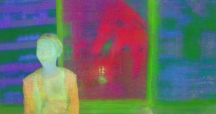
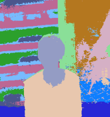
(ii) Input semantic/attention	(d) Our pyr. saliency (volume)	(e) Our merged clustering	(f) Our final foreground	(iv) Extraction (fixed view)

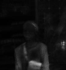
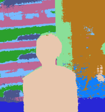
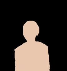
Figure 4: Saliency-aware clustering improves decomposition. On Dynamic Face, the head and body are semantically and saliently different, but are mutually different from the background. This allows us to extract a time-varying 3D field of the object.

4 Experiments

We show the impact of adding semantic and saliency features through scene decomposition and foreground experiments. Our website contains supplemental videos.

Data: NVIDIA Dynamic Scene Dataset (Masked)

This data [45] has 8 sequences of 24 time steps formed from 12 cameras simultaneously capturing video. We manually annotate object masks for view and time step splits; we will release this data publicly. We define three data splits per sequence:

1. Input: A monocular camera that moves position for every timestep is simulated from the input sequences; we use Yoon et al.’s input sequences [45].

2. Fix Cam 0 (hold out): We fix the camera at position 0 as time plays, requiring novel view and time synthesis. $\{(\mathrm{cam}_{0},\mathrm{time}_{i}),i\in[1,2,...23]\}$.

3. Fix Time 0 (hold out): We fix time at step 0 as the camera moves, requiring novel view and time synthesis. $\{(\mathrm{cam}_{i},\mathrm{time}_{0}),i\in[1,2,...11]\}$.

Data: DyCheck Dataset (Masked)

For single-camera casual monocular data, we select a subset of Gao et al.’s DyCheck dataset [10]. We remove scenes without an obvious subject, e.g., where telling foreground from background is hard even for a human. We select haru-sit, space-out, spin, paper-windmill, and mochi-high-five. We uniformly sample $48$ frames and manually annotate object masks. We take even frames as the input set and odd frames as the hold out set. We use the same hyperparameters between both datasets.

Metrics

To assess clustering performance, we use the Adjusted Rand Index (ARI; $[-1,1]$). This compares the similarity of two assignments without label matching, where random assignment would score $\approx$0. For foreground segmentation, we compute IoU (Jaccard), and for RGB quality we use PSNR, SSIM, and LPIPS.

	(a) Input	(b) DINO-ViT (2D)	(c) ProposeReduce [19]	(d) SAFF (Ours; input)	(e) SAFF (Ours; novel)
Dynamic Face
Balloon NBoard
Umbrella

Figure 5: SAFF object segmentations show balanced quality while recovering a volumetric scene representation (e). Basic DINO-ViT produces low-quality segmentations and misses objects. A state-of-the-art 2D video learning method [19] sometimes has edge detail (Umbrella, legs) but othertimes misses detail and objects (Balloon NBoard).

4.1 Comparisons including ablations

SAFF (ours)

We optimize upon the input split of each scene, and perform clustering to obtain object segmentations. To produce a foreground, we merge all salient objects.

SAFF (3D)

The same as above, but processed in 3D rather than on 2D volume projections.

— w/ pyr $\lambda_{\hat{\mathbf{a}}}=\{1,0,0\}$

Pyramid with only coarse saliency (Sec. 3.3) and balanced semantic weight across levels.

— w/o pyr

No pyramid (Sec. 3.3); we optimize with features and saliency extracted from the input image only.

— w/o merge

With pyramid, but we remove cluster merging inside the saliency-aware clustering algorithm.

— w/ blend $v$

To compare generic dynamic segmentation to saliency segmentation, we use the static/dynamic weight instead of volume saliency to segment foreground objects. We set every pixel below the 80% $v$ quantile in each image to be background, or otherwise foreground.

— w/ post process

We add a step after the saliency-aware clustering to refine edges using a conditional random field (please see supplemental material for details). This gains significantly from the depth estimated via volume reconstruction, producing sharp and detailed edges.

NSFF [18] This method cannot produce semantic clusterings. While saliency and blend weight $v$ have different meanings, if we compare our $v$ to NSFF’s, then we can see any impact of a shared backbone with attention heads upon the static/dynamic separation. We disable the supervised motion mask initialization in NSFF as our method does not use such information.

D²NeRF [40] This method also cannot produce semantic clusterings. Over HyperNeRF [26], it adds a shadow field network and further losses to try to isolate objects into the dynamic NeRF over the separate static one. The paper also compares to NSFF without motion mask initialization.

DINO-ViT (2D) [1]

We ignore the volume and pass 2D semantic and attention features into the clustering algorithm. This cannot apply to novel viewpoints. Instead, we evaluate the approach upon all multi-view color images—input and hold-out—whereas other methods must render hold-out views. With our added pyramid processing (Sec. 3.3).

— w/o pyr

No pyramid; upsample to input RGB size.

ProposeReduce (2D) [19]

As a general comparison point, we apply this state-of-the-art 2D video segmentation method. For object segmentation, we use a ProposeReduce network that was pretrained with supervision on YouTube-VIS 2019 [43] for instance segmentation. For foreground segmentation, we use weights pretrained on UVOS [5] intended specifically for unsupervised foreground segmentation. As ProposeReduce is only a 2D method, we provide it with hold-out images for splits with novel views rather than our approach that must render novel views at hold-out poses.

4.2 Findings

	(a) Input	(b) NSFF [18] blend $v$	(c) D2NeRF [40] blend $v$	(d) SAFF blend $v$	(e) SAFF foregrounds
Jumping
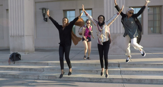
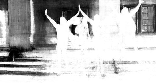
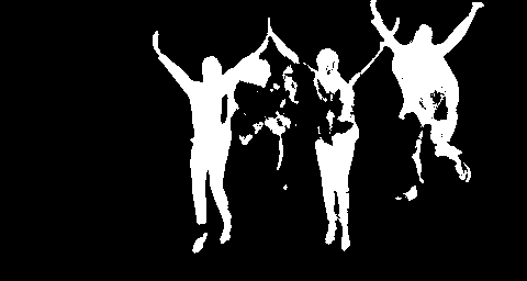
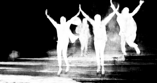
Balloon NBoard

Figure 6: Saliency improves foreground segmentation. Static/dynamic separations are not foreground segmentations, leading to limited use of dynamic NeRF models for downstream tasks. Minor improvements to dynamic blending weight $v$ are seen in some sequences (Jumping) by adding the saliency head to the shared backbone.

Dynamic scene decomposition

We separate the background and each foreground object individually (Tab. 1). The baseline 2D DINO-ViT method is improved by our pyramid approach. But, being only 2D, this fails to produce a consistent decomposition across novel spacetime views even when given ground truth hold-out images. This shows the value of a volume integration. Next, supervised ProposeReduce produces good results (Fig. 5), but sometimes misses salient objects or fails to join them behind occluding objects, and only sometimes produces better edges than our method without post-processing as it can oversmooth edges. ProposeReduce also receives ground truth images in hold-out sets.

Instead, our approach must render hold-out views via the volume reconstruction. This produces more consistent segmentations through spacetime manipulations—this is the added value of volume integration through learned saliency and attention heads. Ablated components show the value of our pyramid step, its coarse-saliency-only variant, and the cluster merge and image post processing steps. Qualitatively, we see good detail (Fig. 5); post-processing additionally improves edge quality and removes small unwanted regions.

Oracle saliency

We also include an oracle experiment where saliency voting is replaced by cluster selection based on ground truth masks. This experiment tells us what part of the performance gap lies with saliency itself, and what remains due to volume integration and cluster boundary issues. With oracle clusters, our decomposition performance is 0.8 ARI (Tab. 1) even in hold-out views. This shows that our existing cluster boundaries are accurate, and that accurate saliency for object selection is the larger remaining problem.

Table 1: Spacetime volume integration improves dynamic scene decomposition. Pyramid construction and cluster merging help quantitatively, and ours is comparable to SOTA supervised 2D video segmentation network ProposeReduce. Metric: Adjusted Rand Index ($[-1,1]$, higher is better).

	Input	Fix Cam 0	Fix Time 0
ProposeReduce (2D)	0.725	0.736	0.742
DINO-ViT (2D)	0.501	0.495	0.321
w/o pyr $\hat{\mathbf{s}},\hat{\mathbf{a}}$	0.470	0.464	0.346
SAFF (3D)	0.594	0.578	0.566
SAFF (ours)	0.653	0.634	0.625
w/ pyr $\lambda_{\hat{\mathbf{a}}}=\{1,0,0\}$	0.620	0.598	0.592
w/o pyr $\hat{\mathbf{s}},\hat{\mathbf{a}}$	0.545	0.532	0.521
w/o merge cluster	0.593	0.574	0.563
w/ post process	0.759	0.733	0.735
w/ oracle	0.834	0.806	0.800
w/ oracle + post process	0.922	0.890	0.880

Table 2: Saliency improves foreground segmentation. Adding saliency also slightly aids how much static/dynamic blend weight $v$ represents the foreground (cf. NSFF blend $v$ to SAFF’s). Here, ProposeReduce uses unsupervised training and data [5]. Metric: IoU/Jaccard ($[0,1]$, higher is better).

	Input	Fix Cam 0	Fix Time 0
ProposeReduce (2D)	0.609	0.464	0.591
DINO-ViT (2D)	0.381	0.382	0.357
NSFF — blend $v$	0.322	0.309	0.268
D2NeRF— blend $v$	0.470	0.334	0.269
SAFF — saliency	0.609	0.589	0.572
— blend $v$	0.388	0.380	0.329
— post process $v$	0.720	0.694	0.679

Foreground segmentation

We simplify the problem and consider all objects as simply ‘foreground’ to compare to methods that do not produce per object masks. Here, the same trend continues (Tab. 2). We note more subtle improvements to static/dynamic blending weights when adding our additional feature heads to the backbone MLP, and overall show that adding top-down information helps produce more useful object masks. Qualitative results show whole objects in the foreground rather than broad regions of possible dynamics (NSFF) or broken objects (D²NeRF; Fig. 6).

Table 3: SAFF semantics generalize to DyCheck Dataset (Masked) Oracle saliency. ProposeReduce is given ground truth test frames, while SAFF must render them. SAFF is comparable to SOTA supervised 2D video segmentation network ProposeReduce. Metric: Adjusted Rand Index ($[-1,1]$, higher is better); IoU/Jaccard index ($[-1,1]$, higher is better).

	ARI		IoU
	Input	Test	Input	Test
ProposeReduce (2D)	0.761	0.762	0.761	0.762
DINO-ViT (2D)	0.801	0.800	0.797	0.797
SAFF (3D)	0.902	0.820	0.910	0.812

Input	ProposeReduce [19]	SAFF (Ours; input)	SAFF (Ours; novel)

Figure 7: SAFF can apply to DyCheck Dataset (Masked). SAFF is comparable to supervised large-scale 2D video learning [19]. Some fine details are improved (bottom, fingers) and novel views maintain their geometry (bottom, gap between legs occluded by head at input timestep).

DyCheck evaluation

DyCheck often has close-up objects and, even with our selected sequences, saliency struggles to find foreground objects. Thus, we use oracle saliency. DINO-ViT and ProposeReduce are given test views while SAFF must render them. Quantitative (Tab. 3) and qualitative (Fig. 7) experiments show similar trends as before: ProposeReduce is good but may miss objects and fine details; SAFF may produce finer details and is more geometrically consistent.

5 Discussion and Limitations

(a) Input	(b) SAVi++ [7]	(c) SAFF

(d) Input	(e) SAFF salient	(f) Salient+dynamic

Figure 8: Limitations. DINO-ViT is not instance-aware, causing unwanted grouping (c). Unwanted static objects may be salient; assuming salient objects are dynamic fixes this (f).

DINO-ViT features are not instance-aware (Fig. 8). This is in contrast to object-centric learning approaches that aim to identify individual objects. To represent these different approaches, we compare to a result from slot-attention based SAVi++ [7]. This method trains on thousands of supervised MOVi [11] sequences with per-object masks, whereas we use generic pre-trained features and gain better edges from volume integration. Combining these two approaches could give accurate instance-level scene objects.

DINO-ViT saliency may attend to unwanted regions. In Figure 8d–e, the static pillars could be isolated using scene flow. But, often our desired subjects do not move (cf. people in Umbrella or Balloon NBoard). For tasks or data that can assume that salient objects are dynamic, we use SAFF’s 4D scene reconstruction to reject static-but-salient objects by merging clusters via scene flow: First, we project $\mathbf{f}$ over each timestep into each input camera pose—this simulates optical flow with a static camera. Clusters are marked as salient per image if mean flow magnitude per cluster $\bar{|\mathbf{p}|}>0.07$ and mean attention $\bar{\mathbf{a}}_{c}>0.07$. Finally, as before, a cluster is globally salient if 70% of images agree (Fig. 8f).

Acknowledgements

The CV community in New England for feedback, and funding from NSF CNS-2038897 and an Amazon Research Award. Eliot thanks a Randy F. Pausch ’82 Undergraduate Summer Research Award at Brown CS.

References

- [1] Shir Amir, Yossi Gandelsman, Shai Bagon, and Tali Dekel. Deep vit features as dense visual descriptors. arXiv preprint arXiv:2112.05814, 2021.
- [2] Jonathan T Barron, Ben Mildenhall, Matthew Tancik, Peter Hedman, Ricardo Martin-Brualla, and Pratul P Srinivasan. Mip-nerf: A multiscale representation for anti-aliasing neural radiance fields. In Proceedings of the IEEE/CVF International Conference on Computer Vision, pages 5855–5864, 2021.
- [3] Kenneth Blomqvist, Lionel Ott, Jen Jen Chung, and Roland Y. Siegwart. Baking in the feature: Accelerating volumetric segmentation by rendering feature maps. ArXiv, abs/2209.12744, 2022.
- [4] Christopher P. Burgess, Loïc Matthey, Nicholas Watters, Rishabh Kabra, Irina Higgins, Matthew M. Botvinick, and Alexander Lerchner. Monet: Unsupervised scene decomposition and representation. ArXiv, abs/1901.11390, 2019.
- [5] Sergi Caelles, Jordi Pont-Tuset, Federico Perazzi, Alberto Montes, Kevis-Kokitsi Maninis, and Luc Van Gool. The 2019 davis challenge on vos: Unsupervised multi-object segmentation. arXiv:1905.00737, 2019.
- [6] Mathilde Caron, Hugo Touvron, Ishan Misra, Hervé Jégou, Julien Mairal, Piotr Bojanowski, and Armand Joulin. Emerging properties in self-supervised vision transformers. In Proceedings of the International Conference on Computer Vision (ICCV), 2021.
- [7] Gamaleldin F. Elsayed, Aravindh Mahendran, Sjoerd van Steenkiste, Klaus Greff, Michael C. Mozer, and Thomas Kipf. SAVi++: Towards end-to-end object-centric learning from real-world videos. In Advances in Neural Information Processing Systems, 2022.
- [8] Zhiwen Fan, Peihao Wang, Yifan Jiang, Xinyu Gong, Dejia Xu, and Zhangyang Wang. Nerf-sos: Any-view self-supervised object segmentation on complex scenes. ArXiv, abs/2209.08776, 2022.
- [9] Xiao Fu, Shangzhan Zhang, Tianrun Chen, Yichong Lu, Lanyun Zhu, Xiaowei Zhou, Andreas Geiger, and Yiyi Liao. Panoptic nerf: 3d-to-2d label transfer for panoptic urban scene segmentation. In International Conference on 3D Vision (3DV), 2022.
- [10] Hang Gao, Ruilong Li, Shubham Tulsiani, Bryan Russell, and Angjoo Kanazawa. Monocular dynamic view synthesis: A reality check. In NeurIPS, 2022.
- [11] Klaus Greff, Francois Belletti, Lucas Beyer, Carl Doersch, Yilun Du, Daniel Duckworth, David J. Fleet, Dan Gnanapragasam, Florian Golemo, Charles Herrmann, Thomas Kipf, Abhijit Kundu, Dmitry Lagun, Issam H. Laradji, Hsueh-Ti Liu, Henning Meyer, Yishu Miao, Derek Nowrouzezahrai, Cengiz Oztireli, Etienne Pot, Noha Radwan, Daniel Rebain, Sara Sabour, Mehdi S. M. Sajjadi, Matan Sela, Vincent Sitzmann, Austin Stone, Deqing Sun, Suhani Vora, Ziyu Wang, Tianhao Wu, Kwang Moo Yi, Fangcheng Zhong, and Andrea Tagliasacchi. Kubric: A scalable dataset generator. 2022 IEEE/CVF Conference on Computer Vision and Pattern Recognition (CVPR), pages 3739–3751, 2022.
- [12] Klaus Greff, Raphael Lopez Kaufman, Rishabh Kabra, Nicholas Watters, Christopher P. Burgess, Daniel Zoran, Loïc Matthey, Matthew M. Botvinick, and Alexander Lerchner. Multi-object representation learning with iterative variational inference. In ICML, 2019.
- [13] Basile Van Hoorick, Purva Tendulka, Dídac Surís, Dennis Park, Simon Stent, and Carl Vondrick. Revealing occlusions with 4d neural fields. 2022 IEEE/CVF Conference on Computer Vision and Pattern Recognition (CVPR), pages 3001–3011, 2022.
- [14] Rishabh Kabra, Daniel Zoran, Goker Erdogan, Loïc Matthey, Antonia Creswell, Matthew M. Botvinick, Alexander Lerchner, and Christopher P. Burgess. Simone: View-invariant, temporally-abstracted object representations via unsupervised video decomposition. ArXiv, abs/2106.03849, 2021.
- [15] Thomas Kipf, Gamaleldin F. Elsayed, Aravindh Mahendran, Austin Stone, Sara Sabour, Georg Heigold, Rico Jonschkowski, Alexey Dosovitskiy, and Klaus Greff. Conditional Object-Centric Learning from Video. In International Conference on Learning Representations (ICLR), 2022.
- [16] Sosuke Kobayashi, Eiichi Matsumoto, and Vincent Sitzmann. Decomposing nerf for editing via feature field distillation. In Advances in Neural Information Processing Systems, volume 35, 2022.
- [17] Abhijit Kundu, Kyle Genova, Xiaoqi Yin, Alireza Fathi, Caroline Pantofaru, Leonidas J. Guibas, Andrea Tagliasacchi, Frank Dellaert, and Thomas Funkhouser. Panoptic neural fields: A semantic object-aware neural scene representation. In Proceedings of the IEEE/CVF Conference on Computer Vision and Pattern Recognition (CVPR), pages 12871–12881, June 2022.
- [18] Zhengqi Li, Simon Niklaus, Noah Snavely, and Oliver Wang. Neural scene flow fields for space-time view synthesis of dynamic scenes. In Proceedings of the IEEE/CVF Conference on Computer Vision and Pattern Recognition (CVPR), 2021.
- [19] Huaijia Lin, Ruizheng Wu, Shu Liu, Jiangbo Lu, and Jiaya Jia. Video instance segmentation with a propose-reduce paradigm. 2021 IEEE/CVF International Conference on Computer Vision (ICCV), pages 1719–1728, 2021.
- [20] Francesco Locatello, Dirk Weissenborn, Thomas Unterthiner, Aravindh Mahendran, Georg Heigold, Jakob Uszkoreit, Alexey Dosovitskiy, and Thomas Kipf. Object-centric learning with slot attention. arXiv preprint arXiv:2006.15055, 2020.
- [21] Kirill Mazur, Edgar Sucar, and Andrew J. Davison. Feature-realistic neural fusion for real-time, open set scene understanding. ArXiv, abs/2210.03043, 2022.
- [22] Luke Melas-Kyriazi, Christian Rupprecht, Iro Laina, and Andrea Vedaldi. Deep spectral methods: A surprisingly strong baseline for unsupervised semantic segmentation and localization. In CVPR, 2022.
- [23] Ben Mildenhall, Pratul P. Srinivasan, Matthew Tancik, Jonathan T. Barron, Ravi Ramamoorthi, and Ren Ng. Nerf: Representing scenes as neural radiance fields for view synthesis. In ECCV, 2020.
- [24] Tom Monnier, Elliot Vincent, Jean Ponce, and Mathieu Aubry. Unsupervised layered image decomposition into object prototypes. In Proceedings of the IEEE/CVF International Conference on Computer Vision (ICCV), pages 8640–8650, October 2021.
- [25] Michael Niemeyer and Andreas Geiger. Giraffe: Representing scenes as compositional generative neural feature fields. In Proc. IEEE Conf. on Computer Vision and Pattern Recognition (CVPR), 2021.
- [26] Keunhong Park, Utkarsh Sinha, Peter Hedman, Jonathan T. Barron, Sofien Bouaziz, Dan B Goldman, Ricardo Martin-Brualla, and Steven M. Seitz. Hypernerf: A higher-dimensional representation for topologically varying neural radiance fields. ACM Trans. Graph., 40(6), dec 2021.
- [27] René Ranftl, Katrin Lasinger, David Hafner, Konrad Schindler, and Vladlen Koltun. Towards robust monocular depth estimation: Mixing datasets for zero-shot cross-dataset transfer. IEEE Transactions on Pattern Analysis and Machine Intelligence, 44(3), 2022.
- [28] Johannes Lutz Schönberger and Jan-Michael Frahm. Structure-from-motion revisited. In Conference on Computer Vision and Pattern Recognition (CVPR), 2016.
- [29] Maximilian Seitzer, Max Horn, Andrii Zadaianchuk, Dominik Zietlow, Tianjun Xiao, Carl-Johann Simon-Gabriel, Tong He, Zheng Zhang, Bernhard Scholkopf, Thomas Brox, and Francesco Locatello. Bridging the gap to real-world object-centric learning. ArXiv, abs/2209.14860, 2022.
- [30] Gyungin Shin, Samuel Albanie, and Weidi Xie. Unsupervised salient object detection with spectral cluster voting. In CVPRW, 2022.
- [31] Cameron Smith, Hong-Xing Yu, Sergey Zakharov, Frédo Durand, Joshua B. Tenenbaum, Jiajun Wu, and Vincent Sitzmann. Unsupervised discovery and composition of object light fields. ArXiv, abs/2205.03923, 2022.
- [32] Karl Stelzner, Kristian Kersting, and Adam R. Kosiorek. Decomposing 3d scenes into objects via unsupervised volume segmentation. ArXiv, abs/2104.01148, 2021.
- [33] Pei Sun, Henrik Kretzschmar, Xerxes Dotiwalla, Aurelien Chouard, Vijaysai Patnaik, Paul Tsui, James Guo, Yin Zhou, Yuning Chai, Benjamin Caine, Vijay Vasudevan, Wei Han, Jiquan Ngiam, Hang Zhao, Aleksei Timofeev, Scott Ettinger, Maxim Krivokon, Amy Gao, Aditya Joshi, Yu Zhang, Jonathon Shlens, Zhifeng Chen, and Dragomir Anguelov. Scalability in perception for autonomous driving: Waymo open dataset. In IEEE/CVF Conference on Computer Vision and Pattern Recognition (CVPR), June 2020.
- [34] Zachary Teed and Jia Deng. Raft: Recurrent all-pairs field transforms for optical flow. In European conference on computer vision, pages 402–419. Springer, 2020.
- [35] Edgar Tretschk, Ayush Tewari, Vladislav Golyanik, Michael Zollhöfer, Christoph Lassner, and Christian Theobalt. Non-rigid neural radiance fields: Reconstruction and novel view synthesis of a dynamic scene from monocular video. 2021 IEEE/CVF International Conference on Computer Vision (ICCV), pages 12939–12950, 2021.
- [36] Vadim Tschernezki, Iro Laina, Diane Larlus, and Andrea Vedaldi. Neural Feature Fusion Fields: 3D distillation of self-supervised 2D image representations. In Proceedings of the International Conference on 3D Vision (3DV), 2022.
- [37] Vadim Tschernezki, Diane Larlus, and Andrea Vedaldi. NeuralDiff: Segmenting 3D objects that move in egocentric videos. In Proceedings of the International Conference on 3D Vision (3DV), 2021.
- [38] Rishi Veerapaneni, John D. Co-Reyes, Michael Chang, Michael Janner, Chelsea Finn, Jiajun Wu, Joshua Tenenbaum, and Sergey Levine. Entity abstraction in visual model-based reinforcement learning. In Leslie Pack Kaelbling, Danica Kragic, and Komei Sugiura, editors, Proceedings of the Conference on Robot Learning, volume 100 of Proceedings of Machine Learning Research, pages 1439–1456. PMLR, 30 Oct–01 Nov 2020.
- [39] Yangtao Wang, Xi Shen, Shell Xu Hu, Yuan Yuan, James L. Crowley, and Dominique Vaufreydaz. Self-supervised transformers for unsupervised object discovery using normalized cut. In Conference on Computer Vision and Pattern Recognition, 2022.
- [40] Tianhao Wu, Fangcheng Zhong, Andrea Tagliasacchi, Forrester Cole, and Cengiz Öztireli. D2nerf: Self-supervised decoupling of dynamic and static objects from a monocular video. ArXiv, abs/2205.15838, 2022.
- [41] Yiheng Xie, Towaki Takikawa, Shunsuke Saito, Or Litany, Shiqin Yan, Numair Khan, Federico Tombari, James Tompkin, Vincent Sitzmann, and Srinath Sridhar. Neural fields in visual computing and beyond. Computer Graphics Forum, 2022.
- [42] Bangbang Yang, Yinda Zhang, Yinghao Xu, Yijin Li, Han Zhou, Hujun Bao, Guofeng Zhang, and Zhaopeng Cui. Learning object-compositional neural radiance field for editable scene rendering. In International Conference on Computer Vision (ICCV), October 2021.
- [43] Linjie Yang, Yuchen Fan, and Ning Xu. Video instance segmentation. 2019 IEEE/CVF International Conference on Computer Vision (ICCV), Oct 2019.
- [44] Vickie Ye, Zhengqi Li, Richard Tucker, Angjoo Kanazawa, and Noah Snavely. Deformable sprites for unsupervised video decomposition. In IEEE Conference on Computer Vision and Pattern Recognition (CVPR), June 2022.
- [45] Jae Shin Yoon, Kihwan Kim, Orazio Gallo, Hyun Soo Park, and Jan Kautz. Novel view synthesis of dynamic scenes with globally coherent depths from a monocular camera. In IEEE/CVF Conference on Computer Vision and Pattern Recognition (CVPR), June 2020.
- [46] Hong-Xing Yu, Leonidas J. Guibas, and Jiajun Wu. Unsupervised discovery of object radiance fields. In International Conference on Learning Representations, 2022.
- [47] Shuaifeng Zhi, Tristan Laidlow, Stefan Leutenegger, and Andrew Davison. In-place scene labelling and understanding with implicit scene representation. In Proceedings of the International Conference on Computer Vision (ICCV), 2021.