Ternary Quantization: A Survey

Abstract

Inference time, model size, and accuracy are critical for deploying deep neural network models. Numerous research efforts have been made to compress neural network models with faster inference and higher accuracy. Pruning and quantization are mainstream methods to this end. During model quantization, converting individual float values of layer weights to low-precision ones can substantially reduce the computational overhead and improve the inference speed. Many quantization methods have been studied, for example, vector quantization, low-bit quantization, and binary/ternary quantization. This survey focuses on ternary quantization. We review the evolution of ternary quantization and investigate the relationships among existing ternary quantization methods from the perspective of projection function and optimization methods.

1 Introduction

Deep neural network (DNN) models involve millions of parameters. Model size and inference efficiency are major challenges when deploying DNN models under latency, memory, and power restrictions. DNN model quantization is very attractive as it can accelerate the training and inference process and lower resource consumption by reducing bit width. Despite these advantages, quantization also poses challenges, especially in training efficiency and performance: i) it takes much more effort to optimize and longer to train than conventional methods; ii) models trained on large datasets usually require pretraining before quantization.

The most significant disadvantage of quantization is that quantized models have lower accuracy than their full-precision counterparts: the lower the bit width, the more noticeable the difference. Binary/ternary quantization are the two extreme cases that can completely replace the multiplication operation with the bit shift operation combined with hardware implementation. Compared with other higher bit-width quantization works (2 to 16-bit), this can bring considerable energy efficiency gains. However, it is hard to maintain a higher accuracy when using binary quantization. The ternary models can achieve much better performance at a small additional bit-width cost. Their performance is comparable with full-precision models. In addition, unlike binary quantization, it is easy to turn a symmetrically higher bit-width quantization into ternary quantization. In other words, ternary quantization is a special case among existing higher bit-width (2-16 bit) symmetric quantization works. Therefore, the summary of ternary quantization works would be instrumental. This survey focuses on ternary weights quantization. Detailed introduction of binary and other quantization works can be found in the work of Amir et al. (2021).

Quantization can be classified in several ways: uniform, nonuniform, symmetric, asymmetric, post-training, and quantization-aware methods. In general, quantization methods involve two steps: thresholding and projection. Therefore, this survey summarizes ternary quantization in terms of projection function and optimization methods. The projection function is categorized by quantization strategies. The optimization methods are categorized by how the gradient is used to optimize the model parameters. We use the proximal operator Neal et al. (2014) to reveal the intrinsic relationship among optimization methods in existing works.

The main contributions of this survey are:

• A holistic and insightful review of ternary quantization.

• A detailed comparison of formulation and optimization during the ternary quantization process.

• Insights into the connections among different ternary quantization methods, which can be generalized to multi-bit quantization.

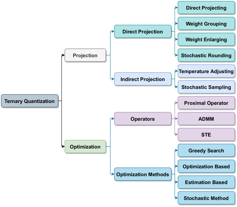
The overall structure of this survey is shown in Figure 1. Section 2 is a brief introduction to ternary quantization. Section 3 describes how ternary quantization is formulated based on projection functions. Section 4 summarizes various optimization methods from the perspective of the proximal operator. Recommendations on potential research topics on ternary quantization and conclusions are in Sections 5 and 6, respectively.

Figure 1: The overall structure of this ternary quantization survey.

2 Ternary Neural Networks

A general representation of a neural network layer is:

$$\small\mathbf{y}=\phi(\mathbf{w}^{\top}\mathbf{x}),$$ (1)

where $\mathbf{w}\in\mathbb{R}^{n\times{m}}$, $\mathbf{x}\in\mathbb{R}^{n}$ is the input vector to the layer, $\phi$ represents a nonlinear activation function, and $\mathbf{y}\in\mathbb{R}^{m}$ is the output feature vector. Ternary quantization has two components, i.e., thresholding and projection:

$$\small\hat{w}=\texttt{Q}(w)=\left\{\begin{aligned} 1&:w>\Delta\\ 0&:\left|w\right|\leq\Delta\\ -1&:w<-\Delta,\end{aligned}\right.$$ (2)

$$s.t.~{}~{}\hat{w}\in\mathbf{\hat{w}},w\in\mathbf{w},~{}\text{and}~{}\Delta\in\mathbb{R},$$

where $\Delta$ denotes the quantization threshold. The optimization objective can be defined as:

$$\small\underset{{\mathbf{w},\alpha}}{\operatorname{argmin}}~{}J(\mathbf{w})=\|\mathbf{w}-\alpha\mathbf{\hat{w}}\|_{2},$$ (3)

where $\alpha$ denotes a scaling factor. Given $\Delta$, $\alpha$ has a closed-form solution Li (2018); Fengfu et al. (2016). More details are in Section 4.1.

2.1 Brief History

Early ternary quantization work aims to deploy models on dedicated hardware. The earliest literature dates back to 1988, in the work of Tzi-Dar and M (1988). Due to hardware limitations, the weights must be quantized into two or three levels in order to program weights onto VLSI chips. The author of Tzi-Dar and M (1988) studies several learning algorithms to project continuous weights into ternary values. It compares six schemes for training a three-layer network with random initialization. They do not explain specific implementation details or outline the workflow. Based on their algorithms and overview, they use a genetic algorithm combined with gradient descent and simulated annealing to solve a ternary weight optimization problem. They claim that the genetic algorithm outperforms other methods.

In 1990, the work of M. et al. (1990) provided a detailed ternary quantization training process. One difference from most modern works is that they do not keep the original copy of full-precision weights but quantize the model immediately after the gradient update. Research efforts were made in the subsequent five years to extend this work. However, the network is elementary, and the data set is small GR and MR (1994); G. et al. (1995). Later, Kyuyeon and Wonyong (2014) tried to use a method similar to Straight-Through Estimator (STE) Yoshua et al. (2013) for quantization. The network is smaller and only has three layers.

Until 2016, with the emergence of Ternary Weight Networks (TWN) Fengfu et al. (2016), ternary quantization began to be used for large models (VGG Karen and Andrew (2014), ResNetKaiming et al. (2016)) and large datasets (ImageNet Jia et al. (2009)). Therefore, those methods designed for simple data and models are no longer applicable. In the early days, TWN and Trained Ternary Quantization (TTQ) Chenzhuo et al. (2016) were relatively intuitive, and the overall accuracy was different from the present ternary quantization methods. Since then, several hardware-related implementations K. et al. (2016); Leroy (2017); Kota et al. (2017); Asit et al. (2017); Li (2018); Giuseppe et al. (2020); Shubham et al. (2020); A. et al. (2020); Peng et al. (2021) have emerged on the basis of TWN and TTQ work. These methods focus on designing hardware; the network is no longer three layers.

Since 2017, some new branches of ternary quantization have been proposed. For example, ternary constrained optimization Cong et al. (2017), knowledge distillation for low-bit models Asit and Debbie (2017), matrix factorization Peisong and Jian (2017), partitioning Aojun et al. (2017, 2018); Peisong et al. (2018) , stochastic quantization Jan et al. (2018); Christos et al. (2018); Oran et al. (2018) , smooth transition Peiqi et al. (2018) and widening Asit et al. (2017). We will elaborate on the development of these methods in the upcoming sections.

2.2 An Overview of Ternary Optimization

The scaling factor $\alpha$ and threshold $\Delta$ in Eq. (3) can be non-symmetric. To obtain ternary weights $\{-\alpha,0,\alpha\}$, most ternary quantization works focus on designing the projection function to make deployment on hardware devices possible. However, ternary quantization usually comes with three problems: the difference between $\mathbf{w}$ and $\mathbf{\hat{w}}$ is significant, the model can get stuck in local minima Amir et al. (2021); Tzi-Dar and M (1988), and the projection brings zero gradients. Therefore, one of the purposes of ternary quantization is to improve the accuracy of the quantized model by narrowing the gap between $\mathbf{\hat{w}}$ and $\mathbf{w}$ Fengfu et al. (2016). In addition, since the projection function will neutralize the gradient update once the magnitude values of updated $\mathbf{w}$ are less than the $\Delta$, the model will stall at the local minimum. Rescaling $\mathbf{w}$ with $\alpha$ can help jump out of these local minimums and thus improve the accuracy of the quantized model GR and MR (1994). Therefore, $\alpha$ and $\Delta$ can reduce the gap between $\mathbf{\hat{w}}$ and $\mathbf{w}$ Fengfu et al. (2016), and jump out of local minimums.

Early work of Tzi-Dar and M (1988) (1988) proposed to jump out of the local minimum by random initialization. The disadvantage is that the old version of weights cannot be used for subsequent training. Therefore, Tzi-Dar and M (1988) further combines the genetic algorithm (GA) to generate a new weight by mixing the stalled weights. The work of M. et al. (1990) was the first one that proposed a scaling factor to alleviate this local minimum problem. The author of M. et al. (1990) projects the full-precision weights to {0, 1, -1}, and then uses $\alpha$ and $\Delta$ to adjust the direction and magnitude of the quantized weights. Their model has only three layers with 132 units. Thus, they use greedy search to obtain the scaling factor $\alpha$ and threshold $\Delta$. Another noteworthy point is that the work of M. et al. (1990) uses full-precision weights only for initialization. Then the gradients are updated directly on the ternary weights, meaning that the full-precision weights are not helpful for the following optimization process.

From the work of Kyuyeon and Wonyong (2014), ternary quantization methods tend to use dual-averaging sub-gradient algorithms Yurii (2002), i.e., updating gradients to full-precision copies rather than ternary weights, which can alleviate the local minima problem caused by projection functions. In this way, the gradients can accumulate on full-precision weights until the magnitude values of $\mathbf{w}$ are greater than the $\Delta$. From another perspective, the intuition of the full-precision update approach is to find the optimal ternary weights near the optimal full-precision weights. Most of the works after 2014 performed gradient updates on full-precision weights and used pre-trained models as initialization when using large-scale datasets, e.g., ImageNet.

After 2014, more and more works take Eq. (3) as a base formula for ternary quantization, which focuses on two parameters, one is the scaling factor $\alpha$, and the other is the threshold $\Delta$. Intuitively, the purpose of these two parameters is actually to make $\mathbf{w}$ and $\mathbf{\hat{w}}$ closer. For example, $\Delta$ and $\alpha$ affect the direction and magnitude of $\mathbf{w}$. The model weights are scaled by $\alpha$, then projected by $\Delta$. The scaling factor $\alpha$ can be a fixed value Fengfu et al. (2016) or an optimized target Chenzhuo et al. (2016). Usually, the threshold $\Delta$ divides $\mathbf{w}$ into zero and non-zero values. It is worth noting that $\Delta$ is usually obtained by estimation rather than optimization. Given $\Delta$, $\alpha$ has a closed-form solution (Eq. (19)). In addition, many works optimize $\alpha$ and $\Delta$ iteratively (See section 4.0.2). Given an estimated $\Delta$, the scaling factor is first calculated by Eq. (19) (like the method in the 90s), and the $\Delta$ is estimated again based on the newer $\alpha$. This process can be repeated several times until the distance between $\mathbf{w}$ and $\mathbf{\hat{w}}$ is small enough. Therefore, we conclude that the scaling factor $\alpha$ and threshold $\Delta$ can optimize the distance between $w$ and $\hat{w}$ and jump out of local minima.

Although $\alpha$ and $\Delta$ can help with ternary projection, projecting continuous variables into discrete spaces leads to the optimization problem of non-differentiable and zero gradients. From the perspective of proximal optimization Neal et al. (2014), proximal gradient descent can be used to approximately solve these problems. The widely used STE also can be seen as a special case of proximal optimization Neal et al. (2014). Most of the optimization process keeps a full-precision copy of the model weights and performs optimization based on the gradients produced by quantization.

This survey covers the ternary quantization works after 2014, as the previous ones are based on small-size networks. The structure of this survey is organized according to the projection function and optimization of ternary quantization.

3 Projection Function

The purpose of the projection function is to produce discrete weight values. Unlike other works that categorize the projection functions into deterministic and stochastic ones, we classify them according to the state of the weights in the forward pass. The following content in this section includes a summary of direct and indirect projection functions. (Note that from this section, the equations in this survey from other works will follow the definitions of the original work, and we will provide the accurate source of such equations.)

3.1 Overview of The Projection Function

For most projection-based ternary quantization methods, the backpropagation gradients are estimated values. Although STE Yoshua et al. (2013) or Hinton’s slides are the most popular, similar methods were used in as early as 1994, in the work of M. et al. (1990). Different from the STE, in the early works, the weights are quantized by the projection immediately after gradient updates. Obviously, the gradient update will be neutralized by projection functions, which brings the problem of getting stuck in local minima Tzi-Dar and M (1988) during training. Until recently, some works have shown that the dual-averaging method Yurii (2002) can alleviate this problem of weight neutralization. The dual-averaging method in the ternary quantization scenario can be interpreted as using projected (quantized) weight values to produce gradients for updating full-precision weights during backpropagation, which is now a widely applied quantization standard.

The purpose of indirect projection methods is to relieve inaccurate gradients by employing a gradual projection process. Some works perform single-element-wise projection, for example, mixing ternary and full-precision values to create hybrid values and gradually adjust the portion of ternary values Yu et al. (2018) or using a temperature-based function to adjust the discrete degree Jiwei et al. (2019); Christos et al. (2018). Other works gradually mix ternary, and full-precision values based on a score function Aojun et al. (2017) or randomly Angela et al. (2020). In addition to the gradual projection methods, stochastic methods either sample discrete weights over the multinomial distribution or add normal-distributed noise to discrete weights to create continuous ones Oran et al. (2018). However, the sampling efficiency of those methods could be a challenge for deep neural networks.

3.2 Direct Projection

Discrete projection uses projection functions to create non-differentiable discrete values in the forward pass. It can be divided into fully and partially discrete methods. Partially discrete methods include group-wise and random discretization. What needs to be considered is how the gradient can be updated to the weight during backpropagation and the solution of corresponding $\alpha$ and $\Delta$. The key factors of ternary quantization are to find the proper scaling factor $\alpha$, threshold $\Delta$, and sub-gradient to minimize the difference between $\mathbf{\hat{w}}$ and $\mathbf{w}$.

3.2.1 Direct Projecting

The earliest direct projection method was mentioned in 1988 Tzi-Dar and M (1988), without any details on the training process.

The first detailed ternary training appeared in 1990 (Eq. (5-8) of M. et al. (1990)):

$$\small\mathrm{E}_{\mathrm{h}}(\mathrm{A})=\sum_{\mathrm{s}}\sum_{\mathrm{k}}\sum_{\mathrm{j}=1}^{\mathrm{N}_{\mathrm{s}-1}}\left(\mathbf{w^{\prime}}_{\mathrm{kj}}^{(s)}-\mathrm{A}^{-1}<\mathbf{w}_{\mathrm{kj}}^{(s)}\mathrm{A}>\right)^{2}$$ (4)

$$\small\mathbf{w^{\prime\prime}}_{\mathrm{kj}}^{(s)}=\left\langle A_{h}\mathbf{w^{\prime}}_{\mathrm{kj}}^{(s)}\right\rangle.$$ (5)

$$\small\mathbf{w^{\prime\prime}}_{\mathrm{kj}}^{(s)}(t+1)=\left\langle\mathbf{w^{\prime\prime}}_{\mathrm{kj}}^{(s)}(t)+\eta\Delta_{k}^{(s)}\right\rangle$$ (6)

where $A$ is the scaling factor, $\langle\cdot\rangle$ denotes rounding, and $\Delta$ is the gradient. We can see that the work of M. et al. (1990) tries to find a proper scaling factor $A$ that minimizes the distance between the scaled $\mathbf{\hat{w}}$ and $\mathbf{w}$. Then use the scaled $\mathbf{\hat{w}}$ for the forward pass. The difference between their method and STE is that Eq. (6) rounds $\mathbf{w}$ directly after the gradient update.

Kyuyeon and Wonyong (2014) project $\mathbf{w}$ into discrete space in the forward pass to produce gradients and keep a full-precision copy of weight values for gradient updates. It also extends the work to higher bit quantization scenarios (Fig 3 and Eq.(5-8) in Kyuyeon and Wonyong (2014)):

$$\small\begin{array}[]{c}{w}_{ij,new}=w_{ij}-\alpha\left\langle\frac{\partial E}{\partial w_{ij}}\right\rangle\\ w_{ij,new}^{(q)}=Q_{ij}\left(w_{ij,new}\right)\\ Q(x)=\Delta\operatorname{sgn}(x)\cdot\min\left\{\left\lfloor\frac{|x|}{\Delta}+0.5\right\rfloor,\frac{M-1}{2}\right\}\end{array}$$ (7)

where $\frac{M-1}{2}$ is the number of bits, $\Delta$ is optimized in a greedy manner, and $\left\langle\cdot\right\rangle$ returns averaged values. The gradient $\frac{\partial E}{\partial w_{ij}}$ is used to update the full-precision $\mathbf{w}$, which is actually the use of STE. Wonyong et al. (2016) use the same quantization method to study the performance gap between the floating point and the ternary weights from the perspective of the model complexity.

Fengfu et al. (2016), the authors of TWN, use STE for quantization in the subsequent work. In their work, the threshold $\Delta$ is an estimated value, and the scaling factor $\alpha$ has a closed-form solution (Eq. (19)). Shen (2018) apply TWN to activation quantization with binary weight values. Yin and Xin (2016) introduce two scaling factors with an estimated $\Delta$ to obtain more accurate ternary values. Yin et al. (2017) restrict the scaling factor $\alpha$ with the form of power-of-two and provide a lower bound of $\alpha$; and it also estimates the $\Delta$ like other works Chenzhuo et al. (2016); Fengfu et al. (2016) do. The work of Hande et al. (2017); Leroy (2017) uses a greedy Dichotomic search to find the optimized $\Delta$, and defines a score function to measure the difference between $\mathbf{w}$ and $\hat{\mathbf{w}}$ (Eq. (3) in Hande et al. (2017)). Wu (2017) propose a preprocessing method based on k-means to assign each weight value to cluster centers, i.e., $\pm\alpha,0$. The scaling factors $\pm\alpha$ play the role of the threshold $\Delta$. The author uses a method similar to TWN to obtain $\alpha$. The final quantization is fulfilled by regular STE.

3.2.2 Weight Grouping

Grouping methods gradually increase the portion of the projected full-precision weights, i.e. $\texttt{Q}(\mathbf{w})$. The advantage of grouping is that using mixed precision weights can bring smaller errors than fully-quantized weights and thus produce more accurate gradients. The error can be measured by:

$$\small\begin{array}[]{c}\|\mathbf{y}-\mathbf{x}^{\top}\mathbf{w}\|_{2}^{2}\leq\|\mathbf{y}-\mathbf{x}^{\top}(r\mathbf{w}+(1-r)\texttt{Q}(\mathbf{w}))\|_{2}^{2}\\ \leq\|\mathbf{y}-\mathbf{x}^{\top}\texttt{Q}(\mathbf{w})\|_{2}^{2},\end{array}$$ (8)

where $r$ controls the projected portion of $\mathbf{w}$. One of the extreme cases can be found in Zijian and Liang (2020):

$$\begin{array}[]{c}\min_{w_{j}}L=\frac{1}{n}\sum_{i=1}^{n}\max\left(0,1-y_{i}\alpha\left(\mathbf{w}_{\neg j}^{\top}\mathbf{z}_{i}+w_{j}z_{ij}\right)\right)\\ +\lambda\alpha^{2}w_{j}^{2}+\lambda\alpha^{2}\mathbf{w}_{\neg j}^{\top}\mathbf{w}_{\neg j},\end{array}$$

$$\small\text{ s.t. }\quad w_{j}\in\{-1,0,1\}$$ (9)

where $\mathbf{z}$ is the input, $L$ denotes the hinge loss, and $\mathbf{w}_{\neg j}$ denotes the full-precision weight vector with $j$-th entry equaling zero. Eq. (9) indicates that: one can perform ternary quantization element by element to obtain optimal ternary weights. Or one can do that reverse; for example, many other methods Aojun et al. (2017); Yiming et al. (2019); Peisong et al. (2018) fix ternary weights but update full-precision weights. The fixed portion of ternary weights is gradually increased during training. The work of Aojun et al. (2017) uses weight magnitude as a reference to fix the ternary weights. Whereas Yiming et al. (2019) use column-wise optimization, i.e., optimizing one column by fixing other columns. Peisong et al. (2018) and Jiwei et al. (2019) perform element-wise and layer-wise quantization, respectively.

In addition, K. et al. (2016) introduce a full-precision buffer zone around $|\pm 0.5|$ and use $h$ to control the width of that zone:

$$\small w(t)=\left\{\begin{array}[]{ll}-1&\text{ if }w_{h}(t)\leq-0.5-h,\\ 0&\text{ if }w_{h}(t)\geq-0.5+h\vee w_{h}(t)\leq 0.5-h,\\ 1&\text{ if }w_{h}(t)\geq 0.5+h,\\ w(t-1)&\text{ otherwise }\end{array}\right.$$ (10)

By setting a continuous zone $[\pm 0.5,\pm h]$, once the weight values in the zone obtain enough gradients, they will have a chance to jump out and become discrete. However, this design cannot guarantee that all weights can jump out. Dubey (2017) combine the concept of grouping with the quantization scheme of TWN. More specifically, the $\mathbf{w}$ is divided into $N$ orthogonal subsets and the optimal $\alpha$ and $\Delta$ are optimized through brute force search (minimizing the $L2$ distance between $\mathbf{w}$ and $\mathbf{\hat{w}}$). The authors of Dubey (2017) also find that grouping through input channels can obtain better ternary quantization results. SYQ (Julian et al. (2018)) proposes a similar method as Dubey (2017) but with a different grouping scheme and optimizes group-wise $\alpha$ with SGD Chenzhuo et al. (2016). Peisong and Jian (2017) decompose the full-precision weight matrix into three subsets in a greedy manner and performs ternary quantization on those subsets; however, the training details are not clear. INQ (Aojun et al. (2017)) quantizes and freezes the full-precision weights with a larger magnitude. The rest flexible weight values are further optimized and gradually quantized. The work of Aojun et al. (2018) defines ternary centers and then gradually increases the quantized portion around the ternary centers. Lukas and Luca (2020) randomly divide the weights into triples and full-precision groups. First, the ternary part is frozen, and the full-precision part is updated. Then the full-precision is frozen, and the ternary is updated to full-precision. Repeat this process and simultaneously increase the proportion of $\mathbf{\hat{w}}$ until quantization is complete.

3.2.3 Weight Enlarging

Duplicating the layer weights Zhezhi et al. (2019) and increasing layer width Asit et al. (2017) can increase the capacity of the model. We name this kind of operation enlarging.

Asit et al. (2017) study the impact of increasing model redundancy, e.g., increasing the layer width and the number of ternary filters, on the accuracy of ternary quantization. Zhezhi et al. (2019) study adding additional ternary residual layers to enhance the model performance. Each layer has multiple copies of the weights, and those copies are empirically assigned with different $\Delta$. Weixiang et al. (2020) produce the ternary by adding two binary weights with scaling factor $\alpha$, which avoids the uncertainty of $\Delta$: $\{\alpha,-\alpha\}+\{\alpha,-\alpha\}=\{2\alpha,0,-2\alpha\}$. Similarly, Yue et al. (2021) stack two ternary weights with coefficients to produce new ternary values.

Hassan et al. (2020) propose a separable ternary structure. Two ternary weights are stacked together as mixed weights during training. The mixed weights can be split into two ternary weights for fast inference. During inference, the two inner products of a layer can be calculated separately but at the cost of doubled computation overhead. Hyungjun et al. (2020) decouple ternary activations into two binary activations by adjusting the bias of the BatchNorm layer. The ternary activations are decomposed into the sum of the two binary ones.

To summarize, enlarging is proposed to compensate for the reduced model capacity caused by ternary quantization. With the use of enlarging, the performance can be improved, but additional computational overhead will also be needed.

3.2.4 Stochastic Rounding

The above-mentioned methods sometimes are usually categorized as deterministic methods. For stochastic methods, an earlier article on stochastic ternary quantization is proposed by Zhouhan et al. (2016), which is an extended work of binary quantization Matthieu et al. (2015). The works of A. et al. (2020) and Hyungjun et al. (2020) show that randomized or stochastic rounding can provide unbiased discrete projection. Zhouhan et al. (2016) apply stochastic ternary quantization in the forward pass, and the power-of-two quantization is applied to the input to eliminate multiplications during backpropagation. Hande et al. (2017) use a pre-trained full-precision (teacher) model to guide the same structure ternary (student) model. It randomly quantizes the teacher activations and then enables the student to imitate these activations by using layer-wise algorithms. The activations are quantized before the weights.

Unlike commonly used methods that obtain gradients in discrete space and update weight in continuous space, in the work of Li (2018), the gradients are stochastically projected into discrete space to update ternary weights. There are six possible transitions for the weight values in total, i.e., $\{-1\}\rightarrow\{0,1\}$, $\{0\}\rightarrow\{-1,+1\}$, and $\{1\}\rightarrow\{-1,0\}$ (see Fig. 3 in Li (2018)). The probability of projection depends on the magnitude and direction of the gradients.

In summary, stochastic rounding selects one of the two closest grid points with probability depending on different measurements, e.g. weight magnitude. Although stochastic rounding can reduce the biased gradient in projection, the sampling speed is slow [ref]. Therefore the efficiency of generating weights is very low, especially when the number of weight elements is large, and the training and inference efficiency of the model will be reduced.

3.3 Indirect Projection

The above-mentioned direct projection methods suffer from non-differentiability. The indirect projection methods try to partially or gradually bypass such non-differentiability. In other words, they try to train a quantized model in the continuous space as much as possible. The indirect projection methods can be categorized into gradual and stochastic discrete projection methods.

3.3.1 Temperature Adjusting

To gradually adjust the discreteness, a common approach is introducing a temperature parameter to a projection function, e.g., tanh Ruihao et al. (2019), Sigmoid Jiwei et al. (2019), and GumbelSoftmax Christos et al. (2018). The higher the temperature, the closer to the step function. The temperature parameter controls the steepness. The temperature adjustment can adapt the strength of discreteness during the quantization.

In the work of Jiwei et al. (2019) and Hassan et al. (2020), the continuous weights pass through a Sigmoid function and become discrete when gradually increasing the temperature of the Sigmoid function:

$$\small\sigma(Tx)=\frac{1}{1+\exp(-Tx)}.$$ (11)

Increasing the temperature $T$ allows the weight values to be gradually converted from continuous to discrete. Peiqi et al. (2018) extend the work of TTQ to RNN and uses a sloping factor to adjust the steepness of activation for quantization. Unlike TWN uses an indicator function directly, the work of Yu et al. (2018) proposes a soft threshold function to fulfill the quantization. More specifically, they propose $L1$ and $L2$ regularizers to adjust the degree of quantization. Then, a gradually increased $\lambda$ is used to adjust the strength of regularizers to convert the full-precision weights to discrete ones. Therefore the ProxQuant Yu et al. (2018) can be seen as a gradual quantization method. The GumbelSoftmax-based method, like Christos et al. (2018), also involves a gradually changed temperature parameter to convert the continuous weights into discrete ones.

3.3.2 Stochastic Sampling

There are two types of stochastic quantization methods. One stochastically projects continuous weight into discrete (Section 3.2.4). And the other stochastic quantization method makes discrete weights continuous again by adding noise to facilitate optimization Jan et al. (2018), or gradually converting stochastic projection from continuous space into discrete space Christos et al. (2018). In the work of Oran et al. (2018), the multinomial distribution is implemented with two Sigmoid functions, and the layer weights are used as the probability parameter, however, at the cost of doubling the weight size. The mean and variance of $\mathbf{\hat{w}}$ are calculated after sampling over multinomial distribution. With the mean and variance value, the noise $\mathcal{N}(0,I)$ is used to generate continuous weights in the forward pass. The discrete weights are obtained during inference by directly sampling over the multinomial distribution (For more details, please see Section 4.2). Christos et al. (2018) use Gumbel-Softmax and temperature parameters. It can be seen as an enhanced version of the LR-net Oran et al. (2018), as it involves a gradually changing temperature as in the Sigmoid-based method. The final form of the weight is discrete, whereas the LR-net directly samples discrete weight during inference, which is inefficient. Stochastic sampling can sample multiple weights to form an ensemble model, however, the overall accuracy could be better.

In summary, the indirect projection has the issue of low running efficiency. The temperature adjusting methods use Sigmoid functions to gradually convert continuous weight to discrete. Accuracy is high, while the training is time-consuming. For example, the quantization method of Jiwei et al. (2019) performs time-consuming layer-wise quantization and has three phases: weight quantization training, activation quantization training with quantized weights, and fine-tuning with both quantized activations and weights together. The training time depends on the depth of the network. The stochastic methods suffer from inefficient sampling – the more parameters the network has, the slower the sampling speed will be.

4 Optimization Methods

The optimization of ternary quantization can be categorized in many ways, for example, optimization-based, estimation-based, and greedy-search-based. One can even use alternative training schemes, knowledge distillation, or additional loss terms to help with the optimization process. We summarize the connections among various forms and use proximal mapping to unify the direct projection optimization methods.

4.0.1 Proximal Operator

Since proximal operators can be viewed as generalized projections Neal et al. (2014), we use the proximal operator to unify ternary quantization methods. In this survey, the proximal operator under ternary settings is:

$$\small\operatorname{prox}_{I_{\texttt{Q}}}(w)=\underset{x\in\mathbb{R},\alpha\in\mathbb{R}}{\operatorname{argmin}}\left(I_{\texttt{Q}}(x)+\frac{1}{2\lambda}\|w-\alpha x\|_{2}^{2}\right),$$ (12)

where $\alpha$ is a scaling factor. If $I_{\texttt{Q}}(x)$ is an indicator function:

$$\small I_{\texttt{Q}}(x)=\left\{\begin{array}[]{ll}0&x\in\texttt{Q}(x),\\ +\infty&x\notin\texttt{Q}(x),\end{array}\right.$$ (13)

then the proximal operator of $I_{\texttt{Q}}$ reduces to Euclidean projection $P(\cdot)$ onto a closed nonempty convex set $\texttt{Q}(x)$:

$$\small P_{\texttt{Q}}(w)=\underset{\alpha,x\in\texttt{Q}(x)}{\operatorname{argmin}}\|w-\alpha x\|_{2}.$$ (14)

Eq. (14) is equivalent to Eq. (3). The optimization process of ternary quantization can be seen as a Euclidean Projection, i.e., projecting full-precision weights into discrete sets $\texttt{Q}(\cdot)$.

4.0.2 Alternating Direction Method of Multipliers

Alternating minimization is commonly used when optimizing with two variables. Ternary quantization can be seen as constrained convex optimization, i.e., a special case of the Alternating Direction Method of Multipliers (ADMM) Stephen et al. (2011). We take the ADMM as a general example to summarize the widely used alternating training scheme in ternary quantization. Consider a generic constrained convex optimization:

$$\small\begin{array}[]{ll}\operatorname{minimize}&f(w)\\ \text{ s.t. }&w\in\texttt{Q}(w).\end{array}$$ (15)

The ADMM form of the above is:

$$\small\begin{array}[]{ll}\text{ minimize }&f(w)+I_{\texttt{Q}}(z)\\ \text{ s.t. }&w-z=0.\end{array}$$ (16)

The training algorithm is described below:

$$w^{k+1} :=\operatorname{prox}_{f}(w)=\underset{w}{\operatorname{argmin}}\left(f(w)+\frac{1}{2\lambda}\left\|w-z^{k}+u^{k}\right\|_{2}^{2}\right),$$ (17)

$$z^{k+1} :=\operatorname{prox}_{I_{\texttt{Q}}}(w)=P_{\texttt{Q}}\left(w^{k+1}+u^{k}\right),$$

$$u^{k+1} :=u^{k}+w^{k+1}-z^{k+1},$$

where $k$ denotes the training iteration. ADMM is most useful when the proximal operators of $f$ and ${I_{\texttt{Q}}}$ can be efficiently evaluated, but the proximal operator for $f+{I_{\texttt{Q}}}$ is not easy to evaluate (See: page 154 of Proximal AlgorithmsNeal et al. (2014)). Therefore, one can easily use the alternating minimization method to perform quantization Kyuyeon and Wonyong (2014); Peisong et al. (2018); Zijian and Liang (2020); Jiwei et al. (2019); Yiming et al. (2019); Lu and T. (2018); Yu et al. (2018); Peisong and Jian (2017). For example, given a specific $\Delta$ and $\alpha$ to optimize $\operatorname{prox}_{f}(w)$, then optimize $\operatorname{prox}_{I_{\texttt{Q}}}$ to get a newer version of $\Delta$ and $\alpha$, repeat this process until the model convergence.

4.0.3 Straight-Through Estimator

The optimization process of ternary quantization with a Straight-Through Estimator is equivalent to a ternary projection function $P_{\texttt{Q}}(w)$ with dual-averaging Yurii (2002):

$$\small\left\{\begin{array}[]{l}{{\hat{w}}}_{t}:=P_{\texttt{Q}}(w)=\underset{\alpha,x\in\texttt{Q}(x)}{\operatorname{argmin}}\|w-\alpha x\|_{2},\\ w_{t+1}=w_{t}-\eta_{t}{\nabla}L\left({\hat{w}}_{t},\right)\end{array}\right.$$ (18)

where $t$ denotes the training iteration, and $\eta_{t}$ denotes the learning rate. When a=1, Eq. (14) becomes very common quantization function, such as A. et al. (2020); Giuseppe et al. (2020); Lukas and Luca (2020); Li (2018); Kota et al. (2017); Zhouhan et al. (2016); K. et al. (2016); Hande et al. (2017); Kyuyeon and Wonyong (2014). Many hardware-quantization articles Peng et al. (2021); A. et al. (2020); Shubham et al. (2020); Giuseppe et al. (2020) also prefer to use this method. However, projecting to $\{\pm 1,0\}$ widens the distance between $\mathbf{w}$ and $\mathbf{\hat{w}}$.

Considering the case of $\alpha>0$, the well-known paper TWN Fengfu et al. (2016) proposes the use of Eq. (14). In addition to the above-mentioned projection $P_{\texttt{w}}$, the work of TWN also uses an approximated $\Delta$ to minimize the optimization objective and then projects $\mathbf{w}$ onto $\alpha\mathbf{\hat{w}}$. Unlike the work of TWN, TTQ Chenzhuo et al. (2016) takes $\alpha$ as an optimized parameter.

4.1 Direct Projection

Direct projection methods usually include $\alpha$ and $\Delta$. In the following content, the works are summarized in three aspects of how to get $\alpha$ and $\Delta$: estimation-based, optimization-based, and greedy-search-based methods.

4.1.1 Estimation Based Methods

The estimation-based methods usually take Eq. (14) as the foundation. As indicated in Eq. (14), the purpose of estimating $\alpha$ and $\Delta$ is finding the shortest $L2$ distance between $\mathbf{w}$ and $\mathbf{\hat{w}}$. Given a fixed $\Delta$, a closed-form solution of $\alpha$ is:

$$\small\alpha=\frac{1}{\|\mathbf{w}\|_{0}}\sum_{i=0}^{n}|w_{i}|.$$ (19)

And the matrix version of Eq. (19) can be found in the work of Cong et al. (2017). One of the drawbacks of estimation-based methods is that there is no explicit solution for the $\Delta$, which causes the $\alpha$ to be inaccurate. Therefore, TWN directly estimates the $\Delta$ with $\frac{0.7}{n}\sum_{i=1}^{n}|w_{i}|$, and TTQ uses $\Delta=0.05\times\operatorname{max}(|\mathbf{w}|)$. As mentioned above, in Eq. (14), when the $\alpha$ is estimated as $1$, the quantization operation is equivalent to projecting the values to $\{0,1,-1\}$ Kyuyeon and Wonyong (2014); Ryan et al. (2021).

Although many works do not mention the form of Eq. (14), according to the definition of proximal mapping, any method with a projection function can be categorized into this estimation-based class. For example, in the ELBNN Cong et al. (2017), the author extends the proximal operator with augmented Lagrange, i.e., a complex projection with ADMM. ELBNN defines the matrix form of $\alpha$:

$$\small\alpha=\frac{\mathbf{w}^{\top}\mathbf{\hat{w}}}{\mathbf{\hat{w}}^{\top}\mathbf{\hat{w}}}=\frac{1}{\|\mathbf{\hat{w}}\|_{0}}\sum_{i=0}^{n}|w_{i}|,$$ (20)

which is identical to Eq. (19).

In addition the projection function, ProxQuant Yu et al. (2018) lets $\alpha=1$ in Eq. (14), like TWN does. The author of Proxquant propose two types of regularization terms, and the quantization function is defined as:

$$\small\mathbf{\hat{w}}=\left\{\begin{array}[]{l}\textsc{SoftThreshold}(\mathbf{w},\mathbf{\hat{w}},\lambda),(L1~{}term),\\ \frac{\lambda\mathbf{\hat{w}}+\mathbf{w}}{1+\lambda},(L2~{}term),\end{array}\right.$$ (21)

where $\lambda$ controls the portion of the quantized weights $\mathbf{\hat{w}}$. Peisong and Jian (2017) mention the scaling factor $\alpha$ should be proportional to the square root of the sum number of rows and columns, however, without any details about the proposed estimation. Aojun et al. (2017) use $2^{n}$ as the scaling factor and perform group-wise quantization in a gradual manner. Shen (2018) use $\Delta=\frac{0.4}{n}\sum_{i=1}^{n}|w_{i}|$ to produce ternary activation. Aojun et al. (2018) add $L1$ and $L2$ regularizers to encourage the weights to move closer to ternary values. The $\alpha$ is estimated by $\texttt{mean}(\mathbf{w})+0.05\texttt{max}(\mathbf{w})$. The training process is sophisticated: the converged full-precision weights are first used to get $\alpha$, then a group-wise quantization is applied. Next, a newer $\alpha$ is obtained, and more weights are quantized group by group. Zhezhi et al. (2019) use $\alpha=\texttt{mean}(\mathbf{w})$ (TWN) and $\Delta=0.05\times\operatorname{max}(|\mathbf{w}|)$ (TTQ) as quantization settings. In addition, they introduce an extra residual layer with independent $\alpha$. Weixiang et al. (2020) add two binary weights to obtain ternary ones and give a closed-form solution of $\alpha$. One of the advantages of the work of Weixiang et al. (2020) is that the $\Delta$ is no longer needed. The author of Weixiang et al. (2020) also proposes refined gradients (Eq. (13) in Weixiang et al. (2020)); however, knowledge distillation is applied in their published code. Therefore, it is hard to know the result without using knowledge distillation.

For the estimation-based works, $\Delta$ controls the number of zeros in $\mathbf{w}$. Given a $\Delta$, $\alpha$ can have a closed-form solution. However, it is hard to explicitly determine $\Delta$ due to the use of learning rate and weight-decay continuously producing a large amount of near-zero values during training. Therefore, if the estimated $\Delta$ is inaccurate, $\alpha$ is inaccurate neither. A proper sparsity can be one consideration during optimizing $\alpha$ and $\Delta$.

4.1.2 Optimization Based Methods

To overcome the abovementioned inaccurate $\alpha$ and $\Delta$ issue, TTQ Chenzhuo et al. (2016) proposes two scaling factors that are optimized by:

$$\small\frac{\partial J}{\partial\alpha^{\pm}}=\sum_{i=1}^{n^{\pm}}\frac{\partial J}{\partial w_{i}^{\pm}},$$ (22)

where “$\pm$” denotes the positive or negative parts. For example, $\alpha^{-}$ denotes the scaling factor for negative weight values $w^{-}$ and is updated by $\sum_{i=1}^{n^{-}}\frac{\partial J}{\partial w_{i}^{-}}$, and $n^{-}$ denotes the number of negative values in $\mathbf{w}$. For the $\Delta$ in TTQ, it has a similar form to TWN, i.e., $\Delta=0.05\times\operatorname{max}(\mathbf{\|w\|_{1}})$, which reveals that $\mathbf{\|w\|_{1}}$ is related to layer sparsity. Therefore, the author of TTQ studies the impact of model sparsity on ternary quantization and concludes that: “Increasing sparsity beyond 50% reduces the model capacity too far, increasing error. The minimum error occurs with sparsity between 30% and 50%.”Chenzhuo et al. (2016). Asit et al. (2017) use the same method as TTQ, but with a widening of the network (WPRN). Peng et al. (2021) introduce a learnable $\Delta$ by replacing it with $\frac{\alpha}{2}$. Julian et al. (2018) group the weight values and assign scaling factors to each group. Then those fine-grained scaling factors are optimized by SGD as TTQ does. Jiwei et al. (2019) formulate the quantization with a Sigmoid function and a temperature coefficient $T$:

$$\small\texttt{Q}(w)=\frac{1}{1+exp(T\times(\beta w+b))},$$ (23)

where $\beta$ and $b$ are learnable coefficients for the quantization parameters $w$. In this way, each parameter can be optimized by SGD (Eq (8-11) of Jiwei et al. (2019)). Yuhang et al. (2019) adopt the same learnable coefficients as Jiwei et al. (2019) by applying: $\bar{w}=\beta w+b,$ where $\beta$ and $b$ are both learned via STE, and then performing ternary quantization. However, Yuhang et al. (2019) does not provide detailed gradient update rules as Jiwei et al. (2019) does. Yue et al. (2021) stack the residual values between the ternary $\mathbf{\hat{w}}$ and $\mathbf{w}$ to obtain a ternary projection function which has the output of $\{-2\alpha,0,2\alpha\}$ and does not need $\Delta$ for thresholding. Moreover, it refines the gradient of $\alpha$ and can be easily extended to arbitrary bits (see Eq. (13-16 and 19) of Yue et al. (2021)).

Ryan et al. (2021) extend the work of TTQ by adding loss regularization terms to mix binary and ternary quantization:

$$\small\min\left(||w|+\alpha|^{p},||w|-\alpha|^{p},\tan(\beta)|w|^{p}\right)$$ (24)

By adjusting $\beta$ from $\frac{\pi}{4}$ to $\frac{\pi}{2}$, they can control the strength of the ternary quantization (Fig. 2 in Ryan et al. (2021)). However, $p$ is empirically set to $1$, and no details are provided regarding optimizing $\beta$ and $\alpha$. Yiming et al. (2019) push the full-precision weights closer to the cluster center (ternary values) by adding regularization terms in the objective function and then using STE for ternary quantization. Lu and T. (2018) add the second-order information (Hessian matrix) term to the objective function to adjust the gradient updates.

4.1.3 Greedy Search Based Methods

Greedy search method is another way to obtain $\alpha$. The works of M. et al. (1990); GR and MR (1994); Hande et al. (2017) use greedy search methods to determine the scaling factor $\alpha$ within a specified range, whereas Kyuyeon and Wonyong (2014) directly search $\alpha$ without a range. Hande et al. (2017) and Leroy (2017) use a half-interval search algorithm to find the best $\pm\alpha$. Wu (2017) uses k-means to continuously update the ternary center of $\mathbf{w}$ after each gradient update. The values of $\mathbf{w}$ are updated with their corresponding center. Then newer centers of $\mathbf{w}$ are calculated for the next training iteration. To make the estimation of $\alpha$ and $\Delta$ in TWN more accurate, Dubey (2017) use two sets of $\alpha$ and $\Delta$ to fulfill quantization and apply brute-force search to obtain them. Specifically, each input channel has an independent scaling factor $\alpha$. Yin et al. (2017) use the power-of-two scaling factor to improve performance further. When the quantization bit is greater than $2$, the $\Delta$ adopts a fixed form of $0.75\times max(||w||_{1})$, which is similar to the estimated $\Delta$ in TTQ. Lu and T. (2018) use the Newton proximal method to facilitate ternary quantization, the second-order information $\mathbf{d}$ is used as a scaling factor when calculating $\alpha$:

$$\small\alpha=\frac{\|\mathbf{\hat{w}}\odot\mathbf{d}\odot\mathbf{w}\|_{1}}{\|\mathbf{\hat{w}}\odot\mathbf{d}\|_{1}}.$$ (25)

A greedy search function $\texttt{find}(\cdot)$ is defined to help obtain $\alpha$. The $\Delta$ is assigned to $\frac{a}{2}$ (Corollary 3.1 in Lu and T. (2018)). Peisong et al. (2018) use greedy search to find optimized $\alpha$. More specifically, during each iteration, it only updates one element of $\mathbf{\hat{w}}$ but fix all the other elements. It only needs to check $n\times 2^{k}$ possibilities, and the bit number $k$ is usually very small. Yiming et al. (2019) minimize a variant of Eq. (3) to encourage weight values to get close to $\{0,\pm\alpha\}$:

$$\small\underset{\alpha,z\in\{0,1\}}{\operatorname{argmin}}\left\|\mathbf{w}-\alpha\mathbf{\hat{w}}^{T}\mathbf{z}\right\|^{2},$$ (26)

$$\small\alpha=\frac{\mathbf{w}\mathbf{z}^{\top}\mathbf{\hat{w}}}{\mathbf{\hat{w}}^{\top}\mathbf{z}\mathbf{z}^{\top}\mathbf{\hat{w}}},$$ (27)

where $\mathbf{z}$ denotes a sparsity indicator vector like a pruning mask. The author of Yiming et al. (2019) defines a greedy function $\texttt{H}(\cdot)$ to solve $\mathbf{z}$, i.e., finding a proper sparsity of $\mathbf{w}$ to obtain optimal $\alpha$. Lukas and Luca (2020) apply group-wise stochastic quantization and gradually increase the quantized portion. During initialization, the pre-trained weights are re-scaled by $\frac{w}{\alpha}$ in order to reduce the $L2$ distance between $\mathbf{w}$ and $\mathbf{\hat{w}}$ (Eq. (5) in Lukas and Luca (2020)). As for finding the optimized $\alpha$, they apply grid search over 1,000 points spread uniformly over $[0,\operatorname{max}(\|\mathbf{w}\|_{1})]$. Zijian and Liang (2020) show a classical proximal mapping quantization. They quantize the SVM model to ternary values. The optimization process does not involve gradient descent (Eq. (9)). Instead, it exhausts all of the possible values of $\{-1,0,1\}$ for each $w$ and selects the value that produces the minor loss.

In summary, although the direct projection is intuitive and convenient, the discrete weights will cause inaccurate gradients. Therefore, based on the proximal operator and the STE, many works propose different refining ideas to relieve the inaccurate gradient issue or get more accurate $\alpha$ and $\Delta$. However, there is no detailed analysis explaining the connection among $\alpha$, $\Delta$, and $\mathbf{w}$. Moreover, there was not any significant improvement in classification accuracy in recent years.

4.2 Indirect Projection

Indirect projection can offset the disadvantage of direct projection based on a statement in the work of Matthieu et al. (2015): K and Giacomo (2015) and Suyog et al. (2015) show that randomized or stochastic rounding can provide the unbiased discrete projection.

In the work of Zhouhan et al. (2016), they use a stochastic method in the forward pass and propose a constraint function $\bar{w}=\texttt{HardSigmoid}(w)$ Matthieu et al. (2015) to ensure $\bar{w}\in\{0,1\}$. In fact, $\bar{w}$ is a parameter of a random value generator. The stochastic quantization process is defined below:

$$\small\begin{array}[]{l}P\left(\hat{w}=1\right)=\bar{w};P\left(\hat{w}=0\right)=1-\bar{w};\text{if}~{}\bar{w}>0\\ P\left(\hat{w}=-1\right)=-\bar{w};P\left(\hat{w}=0\right)=1+\bar{w};\text{if}~{}\bar{w}\leq 0\end{array}$$ (28)

Nevertheless, stochastic quantization can only relieve the inaccurate gradient issue, and the sampling speed is slow when quantizing larger models. Although the experiment result of Zhouhan et al. (2016) is better than the deterministic method, almost all of the following deterministic methods outperform the work of Zhouhan et al. (2016). In addition, the author of Zhouhan et al. (2016) also shows the possibility of quantizing the gradient to 3 to 4 bits during backpropagation. Unlike other works that directly update the full-precision copy of the weight, GXNOR-Net Li (2018) projects the magnitude of gradients to transition probabilities. The stochastic ternary quantization is then controlled by such probability.

The other similar work of Oran et al. (2018) takes $\theta$ as the parameter of the multinomial distribution M() to generate discrete weight values $\hat{w}=\texttt{M}(\theta)$. To make the discrete values $\hat{w}$ continuous again, the author applies the following process:

$$\small\begin{array}[]{l}\mu_{ij}=\mathbb{E}_{\theta_{ij}}\left[\hat{w}_{ij}\right]\text{ and }\sigma_{ij}^{2}=\operatorname{Var}_{\theta_{ij}}\left[\hat{w}_{ij}\right],\\ m_{i}=\sum_{j}\mu_{ij}h_{j}\text{ and }v_{i}^{2}=\sum_{j}\sigma_{ij}^{2}h_{j}^{2}\\ \epsilon\sim\mathcal{N}(0,I),\\ w=m+v\odot\epsilon,\end{array}$$ (29)

where $h$ denotes the input of a layer (Eq. (4) in Oran et al. (2018)). In other words, they apply the reparameterization trick P et al. (2015) to produce continuous weights by using the normally distributed noise $\epsilon$, mean $m_{i}$, variance $v_{i}^{2}$. In this way, the gradients can pass through the projection operation.

Knowledge distillation (KD) can also be used to improve the performance of ternary quantization. Geoffrey et al. (2015) propose the knowledge distillation method to transfer knowledge from a larger neural network (teacher) to a smaller one (student). Applying KD to quantization is proposed by Asit and Debbie (2017); in their work, they compare different scenarios, for example, training the teacher and student network together or training the student with a pre-trained teacher network. In addition to comparing the teacher and student with the same structure, they also compare the scenarios with different structures. Their results show that the KD can significantly improve quantization performance, but applying KD with different network structures and schemes does not bring additional improvement.

5 Opportunities and Future Works

The issue of ternary quantization is low training efficiency and poor accuracy. Most ternary quantization methods using large datasets are trained based on pre-trained models, which is more time-consuming. The lower accuracy is caused by using estimated gradients to update layer weights. Even with increased bit width, the estimation bias in STE still leads to a loss of accuracy since continuous space is essential when performing backpropagation. In addition, the commonly used speedup only works with 16-bit or 8-bit weights, and the hardware implementation for ternary inference has yet to be widely used. Besides, only a few works, such as TTQ et al., study the relationship between the model sparsity and quantization. From a codebook perspective, vector quantization (VQ) and ternary quantization are similar. Ternary can be seen as a special case of fixed codebooks, and more work can be done in this area. Ternary is mainly reflected in the optimization of memory consumption, and the advantage of VQ is mainly reflected in the optimization of hard disk space. The combination of the two can achieve the effect of can optimize both hard disk and memory consumption. There are more ways to design ternary quantization from a stochastic perspective and a generative model perspective.

Another problem is that most works use full-precision weights as initialization to obtain ternary weights. Intuitively, this may need to be revised. Jan et al. (2018) propose a training procedure for constrained full-precision models to obtain very accurate quantized models without training aware quantization. Dan et al. (2023) mention that finding the best full-precision weights around ternary weights and then applying regular ternary quantization can boost the quantization performance. In other words, the current initialization method may need to be adjusted to improve the accuracy. In addition, general quantization methods may emerge in the future.

6 Conclusion

In this survey, we summarize the ternary quantization from the perspective of the projection function and optimization function. We first introduce a brief history of ternary quantization. For example, the origin of the first ternary quantization method and the ternary quantization methods before the introduction of STE. We introduce the projection functions, which include direct projecting, weight grouping, enlarging, stochastic rounding, temperature adjusting, and stochastic sampling. Our classifications provide a new perspective different from conventional classifications, such as uniform, nonuniform, symmetric, and asymmetric quantization methods. Moreover, our classifications are applicable to higher-bit quantization works. We reveal the intrinsic relationship among the ternary quantization methods via proximal optimization. We show how ADMM can explain the widely applied alternating training scheme in ternary quantization. We also examine the connections among STE, dual-averaging, and proximal operators in ternary quantization. This survey summarizes the current research in ternary quantization and provides insight into higher-bit quantization works.

References

- A. et al. [2020] Laborieux A., Bocquet M., Hirtzlin T., Klein J.-O., Diez L. Herrera, Nowak E., Vianello E., Portal J.-M., and Querlioz D. Low Power In-Memory Implementation of Ternary Neural Networks with Resistive RAM-Based Synapse. In 2020 2nd IEEE International Conference on Artificial Intelligence Circuits and Systems (AICAS), pages 136–140, August 2020.
- Amir et al. [2021] Gholami Amir, Kim Sehoon, Dong Zhen, Yao Zhewei, Mahoney Michael W, and Keutzer Kurt. A survey of quantization methods for efficient neural network inference, 2021.
- Angela et al. [2020] Fan Angela, Stock Pierre, Graham Benjamin, Grave Edouard, Gribonval Rémi, Jegou Herve, and Joulin Armand. Training with quantization noise for extreme model compression, 2020.
- Aojun et al. [2017] Zhou Aojun, Yao Anbang, Guo Yiwen, Xu Lin, and Chen Yurong. Incremental Network Quantization: Towards Lossless CNNs with Low-Precision Weights, August 2017.
- Aojun et al. [2018] Zhou Aojun, Yao Anbang, Wang Kuan, and Chen Yurong. Explicit Loss-Error-Aware Quantization for Low-Bit Deep Neural Networks. pages 9426–9435, 2018.
- Asit and Debbie [2017] Mishra Asit and Marr Debbie. Apprentice: Using Knowledge Distillation Techniques To Improve Low-Precision Network Accuracy, November 2017.
- Asit et al. [2017] Mishra Asit, Nurvitadhi Eriko, Cook Jeffrey J., and Marr Debbie. WRPN: Wide Reduced-Precision Networks, September 2017.
- Chenzhuo et al. [2016] Zhu Chenzhuo, Han Song, Mao Huizi, and Dally William J. Trained Ternary Quantization. In arXiv:1612.01064 [cs], December 2016.
- Christos et al. [2018] Louizos Christos, Reisser Matthias, Blankevoort Tijmen, Gavves Efstratios, and Welling Max. Relaxed Quantization for Discretized Neural Networks. In arXiv:1810.01875 [cs stat], October 2018.
- Cong et al. [2017] Leng Cong, Li Hao, Zhu Shenghuo, and Jin Rong. Extremely Low Bit Neural Network: Squeeze the Last Bit Out with ADMM, September 2017.
- Dan et al. [2023] Liu Dan, Chen Xi, Ma Chen, and Liu Xue. Hyperspherical quantization: Toward smaller and more accurate models. In Proceedings of the IEEE/CVF Winter Conference on Applications of Computer Vision, pages 5262–5272, 2023.
- Dubey [2017] Naveen Mellempudi Abhisek Kundu Dheevatsa Mudigere Dipankar Das Bharat Kaul Pradeep Dubey. Ternary Neural Networks with Fine-Grained Quantization, May 2017.
- Fengfu et al. [2016] Li Fengfu, Zhang Bo, and Liu Bin. Ternary Weight Networks, November 2016.
- G. et al. [1995] Hoskins B. G., Haskard M. R., and Curkowicz G. R. A VLSI implementation of multi-layer neural network with ternary activation functions and limited integer weights. In International Conference on Microelectronics, 1995.
- Geoffrey et al. [2015] Hinton Geoffrey, Vinyals Oriol, and Dean Jeff. Distilling the knowledge in a neural network, 2015.
- Giuseppe et al. [2020] Di Guglielmo Giuseppe, Duarte Javier, Harris Philip, Hoang Duc, Jindariani Sergo, Kreinar Edward, Liu Mia, Loncar Vladimir, Ngadiuba Jennifer, Pedro Kevin, Pierini Maurizio, Rankin Dylan, Sagear Sheila, Summers Sioni, Tran Nhan, and Wu Zhenbin. Compressing deep neural networks on FPGAs to binary and ternary precision with HLS4ML, December 2020.
- GR and MR [1994] Curkowicz GR and Haskard MR. A Back-Propagation Adaptation Yielding a Ternary Output ANN with Limited Integer Weights, 1994.
- Hande et al. [2017] Alemdar Hande, Leroy Vincent, Prost-Boucle Adrien, and Pétrot Frédéric. Ternary neural networks for resource-efficient AI applications. In 2017 International Joint Conference on Neural Networks (IJCNN), pages 2547–2554, May 2017.
- Hassan et al. [2020] Dbouk Hassan, Sanghvi Hetul, Mehendale Mahesh, and Shanbhag Naresh. DBQ: A Differentiable Branch Quantizer for Lightweight Deep Neural Networks, July 2020.
- Hyungjun et al. [2020] Kim Hyungjun, Kim Kyungsu, Kim Jinseok, and Kim Jae-Joon. BinaryDuo: Reducing Gradient Mismatch in Binary Activation Network by Coupling Binary Activations, February 2020.
- Jan et al. [2018] Achterhold Jan, Koehler Jan Mathias, Schmeink Anke, and Genewein Tim. Variational Network Quantization. February 2018.
- Jia et al. [2009] Deng Jia, Dong Wei, Socher Richard, Li Li-Jia, Li Kai, and Fei-Fei Li. Imagenet: A large-scale hierarchical image database. In 2009 IEEE conference on computer vision and pattern recognition, pages 248–255. Ieee, 2009.
- Jiwei et al. [2019] Yang Jiwei, Shen Xu, Xing Jun, Tian Xinmei, Li Houqiang, Deng Bing, Huang Jianqiang, and Hua Xiansheng. Quantization Networks, November 2019.
- Julian et al. [2018] Faraone Julian, Fraser Nicholas, Blott Michaela, and Leong Philip H. W. SYQ: Learning Symmetric Quantization for Efficient Deep Neural Networks. pages 4300–4309, 2018.
- K and Giacomo [2015] Muller Lorenz K and Indiveri Giacomo. Rounding methods for neural networks with low resolution synaptic weights, 2015.
- K. et al. [2016] Esser Steven K., Merolla Paul A., Arthur John V., Cassidy Andrew S., Appuswamy Rathinakumar, Andreopoulos Alexander, Berg David, McKinstry Jeffrey L., Melano Timothy, Davis R., Nolfo Carmelo di, Datta Pallab, Amir Arnon, Taba Brian, Flickner Myron D., and Modha Dharmendra S. Convolutional networks for fast energy-efficient neuromorphic computing, 2016.
- Kaiming et al. [2016] He Kaiming, Zhang Xiangyu, Ren Shaoqing, and Sun Jian. Deep residual learning for image recognition. In Proceedings of the IEEE conference on computer vision and pattern recognition, pages 770–778, 2016.
- Karen and Andrew [2014] Simonyan Karen and Zisserman Andrew. Very deep convolutional networks for large-scale image recognition, 2014.
- Kota et al. [2017] Ando Kota, Ueyoshi Kodai, Orimo Kentaro, Yonekawa Haruyoshi, Sato Shimpei, Nakahara Hiroki, Ikebe Masayuki, Asai Tetsuya, Takamaeda-Yamazaki Shinya, Kuroda Tadahiro, and Motomura Masato. BRein memory: A 13-layer 4.2 K neuron/0.8 M synapse binary/ternary reconfigurable in-memory deep neural network accelerator in 65 nm CMOS. In 2017 Symposium on VLSI Circuits, pages C24–C25, June 2017.
- Kyuyeon and Wonyong [2014] Hwang Kyuyeon and Sung Wonyong. Fixed-point feedforward deep neural network design using weights +1 0 and -1. In 2014 IEEE Workshop on Signal Processing Systems (SiPS), pages 1–6, October 2014.
- Leroy [2017] Adrien Prost-Boucle Alban Bourge Frédéric Pétrot Hande Alemdar Nicholas Caldwell Vincent Leroy. Scalable high-performance architecture for convolutional ternary neural networks on FPGA. September 2017.
- Li [2018] Lei Deng Peng Jiao Jing Pei Zhenzhi Wu Guoqi Li. GXNOR-Net: Training deep neural networks with ternary weights and activations without full-precision memory under a unified discretization framework., April 2018.
- Lu and T. [2018] Hou Lu and Kwok James T. Loss-aware Weight Quantization of Deep Networks, February 2018.
- Lukas and Luca [2020] Cavigelli Lukas and Benini Luca. RPR: Random Partition Relaxation for Training; Binary and Ternary Weight Neural Networks, January 2020.
- M. et al. [1990] Marchesi M., Benvenuto N., Orlandi G., Piazza F., and Uncini A. Design of multi-layer neural networks with powers-of-two weights. In 1990 IEEE International Symposium on Circuits and Systems (ISCAS), pages 2951–2954 vol.4, May 1990.
- Matthieu et al. [2015] Courbariaux Matthieu, Bengio Yoshua, and David Jean-Pierre. Binaryconnect: Training deep neural networks with binary weights during propagations, 2015.
- Neal et al. [2014] Parikh Neal, Boyd Stephen, et al. Proximal algorithms, 2014.
- Oran et al. [2018] Shayer Oran, Levi D., and Fetaya Ethan. Learning Discrete Weights Using the Local Reparameterization Trick, 2018.
- P et al. [2015] Kingma Durk P, Salimans Tim, and Welling Max. Variational dropout and the local reparameterization trick, 2015.
- Peiqi et al. [2018] Wang Peiqi, Xie Xinfeng, Deng Lei, Li Guoqi, Wang Dongsheng, and Xie Yuan. HitNet: Hybrid Ternary Recurrent Neural Network. In Advances in Neural Information Processing Systems, volume 31. Curran Associates Inc., 2018.
- Peisong and Jian [2017] Wang Peisong and Cheng Jian. Fixed-Point Factorized Networks. In 2017 IEEE Conference on Computer Vision and Pattern Recognition (CVPR), pages 3966–3974, Honolulu HI, July 2017. IEEE.
- Peisong et al. [2018] Wang Peisong, Hu Qinghao, Zhang Yifan, Zhang Chunjie, Liu Yang, and Cheng Jian. Two-step quantization for low-bit neural networks. In Proceedings of the IEEE Conference on computer vision and pattern recognition, pages 4376–4384, 2018.
- Peng et al. [2021] Chen Peng, Zhuang Bohan, and Shen Chunhua. FATNN: Fast and Accurate Ternary Neural Networks. pages 5219–5228, 2021.
- Ruihao et al. [2019] Gong Ruihao, Liu Xianglong, Jiang Shenghu, Li Tianxiang, Hu Peng, Lin Jiazhen, Yu Fengwei, and Yan Junjie. Differentiable Soft Quantization: Bridging Full-Precision and Low-Bit Neural Networks. pages 4852–4861, 2019.
- Ryan et al. [2021] Razani Ryan, Morin Gregoire, Sari Eyyub, and Nia Vahid Partovi. Adaptive Binary-Ternary Quantization. pages 4613–4618, 2021.
- Shen [2018] Diwen Wan Fumin Shen Li Liu Fan Zhu Jie Qin Ling Shao Heng Tao Shen. TBN: Convolutional Neural Network with Ternary Inputs and Binary Weights, September 2018.
- Shubham et al. [2020] Jain Shubham, Gupta Sumeet Kumar, and Raghunathan Anand. TiM-DNN: Ternary In-Memory Accelerator for Deep Neural Networks, July 2020.
- Stephen et al. [2011] Boyd Stephen, Parikh Neal, Chu Eric, Peleato Borja, Eckstein Jonathan, et al. Distributed optimization and statistical learning via the alternating direction method of multipliers, 2011.
- Suyog et al. [2015] Gupta Suyog, Agrawal Ankur, Gopalakrishnan Kailash, and Narayanan Pritish. Deep learning with limited numerical precision. In International conference on machine learning, pages 1737–1746. PMLR, 2015.
- Tzi-Dar and M [1988] Chiueh Tzi-Dar and Goodman Rodney M. Learning algorithms for neural networks with ternary weights, 1988.
- Weixiang et al. [2020] Xu Weixiang, He Xiangyu, Zhao Tianli, Hu Qinghao, Wang Peisong, and Cheng Jian. Soft Threshold Ternary Networks. volume 3, pages 2298–2304, July 2020.
- Wonyong et al. [2016] Sung Wonyong, Shin Sungho, and Hwang Kyuyeon. Resiliency of Deep Neural Networks under Quantization, January 2016.
- Wu [2017] Jie Ding JunMin Wu Huan Wu. Three-Means Ternary Quantization. November 2017.
- Yiming et al. [2019] Hu Yiming, Li Jianquan, Long Xianlei, Hu Shenhua, Zhu Jiagang, Wang Xingang, and Gu Qingyi. Cluster Regularized Quantization for Deep Networks Compression. In 2019 IEEE International Conference on Image Processing (ICIP), pages 914–918, September 2019.
- Yin and Xin [2016] Penghang Yin and Yingyong Qi Shuai Zhang Jack Xin. Training Ternary Neural Networks with Exact Proximal Operator, December 2016.
- Yin et al. [2017] Penghang Yin, Zhang Shuai, Qi Yingyong, and Xin Jack. Quantization and training of low bit-width convolutional neural networks for object detection, 2017.
- Yoshua et al. [2013] Bengio Yoshua, Léonard Nicholas, and Courville Aaron. Estimating or propagating gradients through stochastic neurons for conditional computation, 2013.
- Yu et al. [2018] Bai Yu, Wang Yu-Xiang, and Liberty Edo. ProxQuant: Quantized Neural Networks via Proximal Operators. September 2018.
- Yue et al. [2021] Li Yue, Ding Wenrui, Liu Chunlei, Zhang Baochang, and Guo Guodong. TRQ: Ternary Neural Networks With Residual Quantization, May 2021.
- Yuhang et al. [2019] Li Yuhang, Dong Xin, Zhang Sai Qian, Bai Haoli, Chen Yuanpeng, and Wang Wei. RTN: Reparameterized Ternary Network, December 2019.
- Yurii [2002] Nesterov Yurii. Primal-dual subgradient methods for convex problems, 2002.
- Zhezhi et al. [2019] He Zhezhi, Gong Boqing, and Fan Deliang. Optimize Deep Convolutional Neural Network with Ternarized Weights and High Accuracy. In 2019 IEEE Winter Conference on Applications of Computer Vision (WACV), pages 913–921, January 2019.
- Zhouhan et al. [2016] Lin Zhouhan, Courbariaux Matthieu, Memisevic Roland, and Bengio Yoshua. Neural Networks with Few Multiplications. In International Conference on Learning Representations, February 2016.
- Zijian and Liang [2020] Lei Zijian and Lan Liang. Memory and Computation-Efficient Kernel SVM via Binary Embedding and Ternary Model Coefficients, October 2020.