An Adaptive Computational Intelligence Approach to Personalised Health Assessment and Immune Age Characterisation from Common
Hematological Markers

Abstract

We introduce a simulated digital model that learns a person’s optimal blood health over time. Using a learning adaptive algorithm, our model provides a risk assessment score that compares an individual’s chronological age from birth to an estimation of a biological immune age derived from the score. We demonstrate its efficacy against real and synthetic data from medically relevant cases, extreme cases, and empirical blood cell count data from 100K data records in the Centers for Disease Control and Prevention’s National Health and Nutrition Examination Survey (CDC NHANES) that spans 13 years. We find that the score is informative when distinguishing healthy individuals from those with diseases, both self-reported and abnormal blood tests manifested, providing an entry-level score for patient triaging. We show that, by analyzing an individual’s Full Blood Count (FBC) or Complete Blood Count (CBC), test results over time allows us to calculate an immune age score that correlates with chronological age. The immune age score, derived solely from popular hematological markers, can be widely used to serve purposes of precise healthcare, and predictive medicine.

Keywords: personalized health, predictive medicine, twin digital health, blood risk score, risk stratification, individual assessment, immune age

1 Introduction

Risk assessment tools are often needed to improve patient safety and patient outcomes. Risk assessment scores used for initial patient classification or diagnosis and triaging (i.e., assessment of priority for healthcare services) are often qualitative and inter-subjective. Robust quantitative tools with clinical relevance are required to optimize health monitoring choices across all levels of healthcare systems.

Risk scores are valuable predictive tools that, when implemented, can be utilised by clinicians with positive results, leading to better patient outcomes. Risk assessment measures for patient triage are often needed to optimise patient pathways and health monitoring across all levels of health care. However, most scores are defined for very specific conditions, such as heart disease, cardiovascular disease (CVD) or venous thromboembolism (VTE), to mention just a few. Others reflect factors such as risk of severe disease [23, 31], clinical acuity [10, 33], and long-term outcomes [30, 32]. For example, the Intermountain risk score [19] provides a complete / full blood count (CBC / FBC) risk score shown to be associated with bleeding and in-hospital mortality based on red blood cell size, originally used as an anaemia predictor [26], and is often reported in FBC/CBC panels.

FBC/CBCs have been found to contain enough information to produce clinically useful scores [3, 18]. At the same time, it has also been shown that although a CBC is a low-cost laboratory test that is almost universally used, its risk predictive information content is often underused [29].

Regular blood testing has been associated with short-term mortality and with the ability to significantly improve emergency department triage [22]. Most risk scores depend on multiple factors external to a single test result in itself and have proven useful when available, even in the context of the immune system [34]. A number of these scores are based on such factors as physiological data, medical and family history, and lifestyle choices, and reference a range of things, from age and sex to drinking and smoking habits. While numerical scores and colour-based scores are relatively common, to the authors’ knowledge no single general numerical and colour-based blood test risk assessment score exists that is based on a combination of distances from population or personalised average values, in particular for CBC and immune-related data.

In medical practice, a simple risk score based solely on blood test results and agnostic with respect to a specific condition while still being able to quantify the results of a blood test has not been proposed, to the authors’ knowledge. Here we introduce a general numerical and colour-based risk stratification score to quantify any number of abnormal blood markers. The risk model introduced is not data expensive when run ab initio, and yet it is shown to be informative, and its implementation is easily interpretable, while allowing for adaptation to enhance sophistication.

A marker, analyte or test parameter is a potentially non-mutually exclusive property related to a blood test. Analytes can include protein-based substances, antibodies, biochemical entities and any other product or sub-product of cellular function related to the blood or to the immune system. For example, in a Full (or Complete) Blood Count, there are usually about 13 to 15 analytes, although the proposed score is not limited to any particular set or number of such analytes. In the context of a cell’s properties, relevant tests can index, for example, cell count, cell size, cell morphology, cell nuclei morphology and cell maturity, among a wide range of parameters/analytes.

2 Methods

Here we introduce a family of indices based on a distance metric and closed learning algorithm for detecting rapid, small (precise), and personalised changes in blood test results. The indexes have the advantage of being fully explainable, unlike those featured in other statistical or machine-learning approaches. This metric takes the form of a quantitative measure or score that aggregates data from a set of numeric blood test results, combining and condensing them into a single numerical value that allows rapid triage, sorting, and immune age assessment. The main purpose of the score is to learn from, monitor, and provide a quick assessment of divergence from population and personalised reference values.

We will call this risk assessment score ”immune score”, given its connection to the immune system through blood cell subpopulation counts, in particular as registered in the most popular blood test, the FBC or the CBC.

The immune score constitutes a dimensional reduction technique based on a single real-value number and a colour scheme that takes a multidimensional blood test space with dimension size equal to the number of analytes, where each value of a marker or analyte corresponds to the coordinate of that value in that dimension. The score itself can be seen as the norm of a suitable vector transformation that pinpoints the health status of the patient in that space, relative to the test and the set of markers or analytes. Thus, the numerical vector value integrates all the analyte’s space dimensions.

Let

$$\bar{x}=(x_{1},\dots,x_{n})$$

be a vector of raw analyte values obtained by a suitable (series of) lab tests, as usually presented to physicians and patients.

We call the associated vector space for blood cell analytes the multidimensional immune space, or the immune space for short.

CDC NHANES data were used to estimate deficiencies and toxicities of specific nutrients in the population and subgroups in the U.S., to extract population reference data, and to estimate the contribution of diet, supplements, and other factors to whole blood levels of nutrients. This data can be used for research purposes and is publicly available [28].

2.1 Numerical score

This first formulation of the score takes the form of a linear function because it does not take into account possible interactions between analytes. CBC blood cell counts can interact through immune system responses. For example, an infection may increase neutrophils and decrease lymphocytes. RBC parameters can also be impacted by complex environmental cues such as nutrient levels, iron deficiency, stress conditions, or disorders. We also assume that each analyte contributes equally to the immune score (this is likely to be only partially true, as some of the analytes are more or less medically informative than others, with this degree of informativeness itself varying with different conditions. Moreover, not all analytes are independent, and some analytes may be statistically dependent on others—suitable refinements will be introduced later). Some examples of analytes which are independent of each other are RBC and WBC count (they do not directly influence the counts of each other). The counts of some analytes are dependent of each other. Examples include Neutrophils and WBC. In essence, neutrophils are a type of leukocyte (WBC), so the neutrophil count is included in and contributes to the total WBC. Another example is Hemoglobin and hematocrit. Hemoglobin measures the amount of hemoglobin protein in red blood cells. Hematocrit measures the percentage of blood volume taken up by red blood cells. Thus, Hematocrit is mathematically dependent on the hemoglobin concentration because one gives a subset or ratio of the other.

For ease of comparison between successive versions of the score, all values are normalized within the range $[0,10]$. Following user feedback, we then reverse the scale by subtracting the normalized value from 10. This means that each analyte will contribute with a maximum weight of

$$w_{a}=\sqrt{\frac{100}{N}}.$$

where $N$ is the number of analytes. From now on we will consider the example of $N=13$ typical for a CBC or FBC. Before the scale inversion, from a geometrical point of view a vector of values in the multidimensional immune space will be mapped to a point in a $N$D-“quadrant” going from 0 to $w_{a}$ that will be called the normalised immune space. This mapping will allow us to observe the evolution of an individual’s score as a trajectory in the normalised immune space where a notion of distance will come in handy.

While the score proposed is agnostic, in the sense that it can incorporate, or not, any number of analytes, and requires no other input, it can be adapted to incorporate medically relevant information by assigning weights that serve as multipliers of an analyte’s effect according to its criticality for different profiles.

The adoption of a score within a maximum range of $[0,10]$ can be approached in different ways. One is to assume no theoretical maximum values for analytes and asymptotically approach the minimum score of 0, without ever reaching it in individual cases. We adopted an alternative approach, capping values to a pre-established “reasonable” maximum, beyond which all specific values mean the same. The pre-established maximum is two standard deviations beyond normal (healthy) ranges, which sets the statistical significance critical value alpha at 0.05 (i.e., 95% confidence interval).

In an initial test, reference tables from Haematology Reference Ranges from the NHS were used for normal (healthy) ranges for each analyte according to age, sex, and pregnancy status [7]. $G$ will denote the set of possible categories:

$G$	=	$\{$Adult male, non-pregnant adult female, pregnant adult female,
		newborn child, two-month-old child, six-month-old child,
		one-year old child, 2-6-year-old child, 6-12-year-old child, 12-18-year-old teenager$\}$

Let $g$ denote any value in $G$.

For each analyte, $r_{u}(g,i)$ is the upper limit in the normal range of the analyte $i$ for an individual belonging to group $g$. Similarly, $r_{l}(g,i)$ is the lower limit.

An efficient computer implementation of the score can pre-calculate the following values:

• The expected vector, containing the mean value of each analyte for a given group:

  $$\bar{e}(g)=(e(g,1),\dots,e(g,N)).$$

  Mean values will derive from the analysis of suitable data to be obtained from reliable databases or directly collected by us. For ease of explanation, in the following we provisionally select the arithmetical average of the lower and upper limits in the NHS table:

  $$e(g,i)=\frac{r_{l}(g,i)+r_{l}(g,i)}{2}.$$

• The standard deviation for an analyte $i$ in group $g$ is denoted by

  $$\sigma(g,i).$$

  Again, these values will be empirically calculated. In the meantime, we will use the distance from the mean to either limit within the normal (healthy) range:

  $$\sigma(g,i)=\frac{(r_{u}(g,i)-r_{l}(g,i))}{2}.$$

• The maximum difference vector, containing the maximum possible distance from the mean value of each analyte:

  $$\bar{m}(g)=(m(g,1),\dots m(g,N)),$$

  where

  $$m(g,i)=\frac{(r_{u}(g,i)-r_{l}(g,i))}{2}+2\sigma(g,i).$$

  (twice standard deviations from the limits of the healthy ranges).

• The weighted vectors of each group (which will be used to normalise the possible values to a maximum immune score, before reversion, of 10):

  $$\bar{w}(g)=(w(g,1),\dots,w(g,N)),$$

  where $w(g,i)=w_{a}/m(g,i)$.

Let $\bar{c}=(c_{1},\dots,c_{N})$ be a vector of analyte values for an individual of group $g$. Then the normalised vector is calculated using the following formula:

$$\bar{n}(\bar{c})=(f(c_{1},e(g,1),m(g,1),w(g,1)),\dots,f(c_{N},e(g,N),m(g,N),w(g,N))),$$

where

$$f(x,y,z,w)={\sf if}\>|x-y|\geq z\>{\sf then}\>w_{a}\>{\sf else}\>|x-y|\times w.$$

The value obtained by subtracting the normalized vector $\bar{n}(\bar{c})$ from 10 is defined as the Normalized Immune Score, abbreviated as NIS:

$$\text{NIS}=10-\|\bar{n}(\bar{c})\|.$$

We will denote the uninverted score by $\text{NIS}^{*}$, which is defined as $\text{NIS}^{*}=\|\bar{n}(\bar{c})\|$.

One novel aspect of this metric is the ability to incorporate medical knowledge into the score calculation using weights (scalar or piecewise functions). This allows adding clinical expertise to the data-driven score in a transparent mathematical way, rather than using opaque statistical black-box approaches. Statistical black-box approaches refer to complex statistical modeling techniques that are not easily interpretable (e.g., neural networks). The weights make it possible to adjust analyte contributions in a nonlinear fashion if needed. Synthetic analytes can also be introduced to simulate nonlinear relationships in a clear mathematical form, rather than dealing with nonlinearities directly in a statistically obscure way. Unlike statistical or machine learning approaches, the distance-metric-based score is transparent, so that clinicians can fully understand how it works, and even reproduces the calculation by hand with a justification at every step without loss of generality.

2.2 Colour-based score

In addition to this numerical value, the score incorporates a second indicator that will be easy to read and interpret. The idea is to utilise colour codes as a means of flagging deviations from normal (healthy) reference values. This is called the Colour-Coded Immune Score or CCIS for short.

The CCIS uses the same analytes and their normal (healthy) ranges as before. There are thresholds for each of the analytes that trigger different types of alerts:

• A value within normal healthy ranges: No alert, colour coded green.

• An abnormal value within one standard deviation above/below healthy reference values: amber alert.

• An abnormal value beyond one standard deviation from the normal healthy values: red alert. As in the normalised immune score, values are capped to a maximum of two standard deviations.

Keeping the range to within two standard deviations when assessing a score or metric has the following statistical implications: 1) About 95% of observations fall within 2 standard deviations of the mean in a normal distribution. Thus, restricting the range cuts off the most extreme 5% of outliers. This makes the statistics more robust by removing very unusual values (outliers) that could skew results. But it also reduces the variability seen in the data. However, it may also provide an overly narrow or skewed view of the true variability in the metrics being evaluated. For the goals of our analysis, i.e., sample CBC analysis, assuming a normal distribution justifies this rationale and its implications.

The results for each analyte are also combined in a single global value, which will constitute the CCIS. The rules are as follows:

• Green: all values within normal range (green).

• Amber: 1-3 individual amber alerts.

• Red: More than 3 amber alerts or one or more red alerts.

Clearly, the CCIS is not a numerical value, but a colour-coded output, like the individual alerts for separate analytes. This clearly distinguishes the CCIS from the normalised immune score.

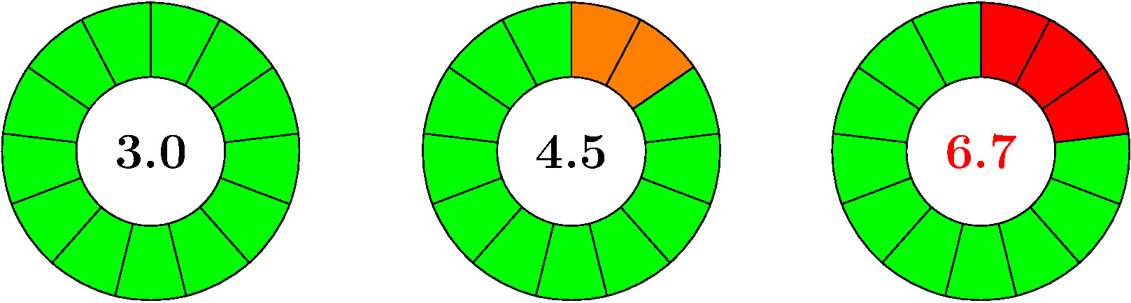
The information for the CCIS can be presented in a simple graphical way. We construct a doughnut graph with one slice for each analyte. Analytes assigned the same colour will be grouped together, which will produce doughnut graphs of at most 3 different colour-coded sections. Some examples for purposes of illustration are presented in Fig. 1.

3 A numerical score derived from the CCIS

We explored an alternative score that would follow the colour-coded scheme, but would also produce a numerical value. The intention was to combine the accessibility of the CCIS and the finer precision of the NIS in a single value. As with the latter, the value would range from 0 to 10.

We expected the following property: If $v_{1},v_{2}$ are possible score values and $v_{1}>v_{2}$, it should be the case that $v_{2}$ indicates greater cause for concern than $v_{1}$.

On the other hand, values should be closely related to the colour codes. That is, values $v_{1}$, $v_{2}$ and $v_{3}$ correspond to CCIS scores of green, amber and red, respectively, and they should be ordered as follows:

$$v_{1}>v_{2}>v_{3}.$$

A more precise way of expressing the above ideas is the set of rules codified in Table 3.

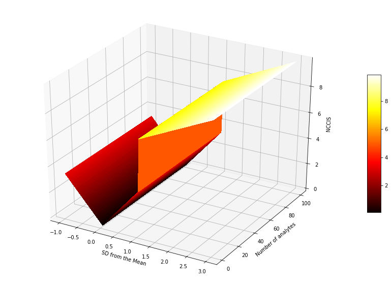
In the following section, we present a procedure for translating the CCIS into a numerical value according to the above schema. We will call this value the NCCIS. The expected behaviour of the NCCIS with respect to the number of analytes and its deviation from the norm can be observed in Fig. 3.

Table 1: NHS reference values: Typical tabular presentation for illustration purposes of a Complete/Full Blood Count test. Minimum and maximum value show minimum and maximum between male/female values.

Parameter/Component	Result	Low Ref Value	High Ref Value
Haemoglobin (HgB)	152.3 g/L	115 g/L	180 g/L
Total White Cell Count (WBC)	9.3 g/L	3.6 g/L	11.00 g/L
Platelet count (PLT)	286.5 $\times 10^{9}$/L	140 $\times 10^{9}$/L	400$\times 10^{9}$/L
Red cell count	5.5 $\times 10^{12}$/L	3.8$\times 10^{12}$/L	6.5$\times 10^{12}$/L
Mean Cell Volume (MCV)	93.3 fL	80 fL	100 fL
MC Haemoglobin (MCH)	29 pg	27 pg	32 pg
MCH Concentration	315 g/L	310 g/L	350 g/L
Neutrophils	6.9 $\times 10^{9}$/L	1.8 $\times 10^{9}$/L	7.5$\times 10^{9}$/L
Lymphocytes	3.6$\times 10^{9}$/L	1.0$\times 10^{9}$/L	4.0$\times 10^{9}$/L
Monocytes	0.3$\times 10^{9}$/L	0.2 $\times 10^{9}$/L	0.8 $\times 10^{9}$/L
Eosinophils	0.2$\times 10^{9}$/L	0.1$\times 10^{9}$/L	0.4$\times 10^{9}$/L
Basophils	0.2$\times 10^{9}$/L	0.02 $\times 10^{9}$/L	0.1$\times 10^{9}$/L
Haematocrit	0.4 L/L	0.37 L/L	0.47 L/L

Table 2: Mean values and standard deviations found in the NHANES 2003–2016 database for the 13 analytes of the immune scores (same units as above).

Analyte	Mean Male	Std Male	Mean Female	Std Female
Haemoglobin (HgB)	150.72	11.51	133.33	11.62
Total White Cells	6.92	3.12	7.01	2.09
Platelet count (PLT)	228	54.33	255.42	64.19
Total Red Cells (RBC)	4.93	0.45	4.40	0.38
MCV	89.96	5.13	89.22	5.72
Hematocrit (HT)	0.44	0.03	0.39	0.03
MCH	26.96	10.33	26.55	10.47
MCHC	336.55	18.41	335.02	20.46
Neutrophils	4	1.85	4.16	1.66
Lymphocytes	2.11	2.21	2.11	0.79
Monocytes	0.57	0.21	0.52	0.18
Eosinophils	0.20	0.16	0.17	0.14
Basophils	0.04	0.06	0.04	0.05

The behaviour of Fig. 3 illustrates how values at a remove from healthy values are pushed towards higher values by design, as an alerting mechanism.

3.1 Calculating CCIS and NCCIS

The computation of NCCIS is performed using the uninverted $\text{NIS}^{*}$. Some of the values used in the calculation of the $\text{NIS}^{*}$ include:

• $w_{a}=\sqrt{100/13}$ is the maximum normalised distance for each analyte in the normalised vector of a patient’s readings.

• $e(g,i)$ is the mean (or expected) value for analyte $i$ in group $g$.

• $\sigma(g,i)$ is the standard deviation from the mean.

• $n(g,i)=(r_{u}(g,i)-r_{l}(g,i))/2$ is the normal (healthy reference) interval length from the mean value (assuming upper and lower limits are equidistant from the mean, an assumption to be revised in the future, both in the NIS and here in the NCCIS).

Now the raw (not normalised) borders between colours are

• raw maximum value for green: $n(g,i)$.

• raw maximum value for amber: $n(g,i)+\sigma(g,i)$.

• raw maximum value for red: $n(g,i)+2\sigma(g,i)$.

And the normalised version:

$$m_{gr}(g,i) = n(g,i)\times(w_{a}/(n(g,i)+2\sigma(g,i)))$$

$$m_{a}(g,i) = (n(g,i)+\sigma(g,i))\times(w_{a}/(n(g,i)+2\sigma(g,i)))$$

$$m_{r}(g,i) = (n(g,i)+2\sigma(g,i))\times(w_{a}/(n(g,i)+2\sigma(g,i)))=w_{a}$$

Therefore the current $\text{NIS}^{*}$ intervals for the different colours for individual analytes are:

• Green: $[0,m_{gr}(g,i)]$ (that is, from 0 distance from the mean value up to the normalised maximum value for green.)

• Amber: $(m_{gr}(g,i),m_{a}(g,i)]$.

• Red: $(m_{r}(g,i),w_{a}]$.

Figure 1: CCIS colour-based alerts. On the left, an individual with all values normal (healthy) and thus coded green. At the centre, an individual with two amber alerts. On the right-hand side, an individual with three red alerts, which produce a global red flag quantifying potential risk by colouring the numerical score depicted in the centre. In applications, colours following the guidelines of national health systems such as the NHS are recommended. For convenience, the numerical score has been inverted (with respect to $\text{NIS}^{*}$) to conform to the popular 0-10 grading scheme, where 10 is best and 0 is worst.

For global values the calculation has to take into account both the definition of the $\text{CCIS}^{*}$ and the fact that each analyte can have proportionally different normal ranges and standard deviations:

• Green: The minimum global green corresponds to 0 in every analyte. The maximum is $m_{gr}(g,i)$ in each analyte. This gives us the following interval:

  $$[0,\sqrt{\sum^{13}_{i=1}m_{gr}(g,i)^{2}}]$$

• Amber: The minimum global amber is 1 analyte value, just above green. The maximum is 3 maximum amber values and the rest (10) at the upper limit of green. Let analyte $j$ be such that $m_{gr}(g,j)$ is the minimum of the green upper limits, and let analytes $k$, $m$, $n$ be the three biggest of the amber upper limits. Then we have the following interval:

  $(m_{gr}(g,j),$

  $\quad\sqrt{(m_{a}(g,k)^{2}+m_{a}(g,m)^{2}+m_{a}(g,n)^{2})+m_{gr}(g,i_{1})^{2}+\cdots m_{gr}(g,i_{10})^{2}}].$

• Red. The minimum global red is 1 red analyte value or 3 amber analyte values. The maximum is, obviously, 10 (13 maximum individual analyte values). Let us suppose that the lowest minimum for red is $(m_{r}(g,k))$ and that there are no 3 upper limits for amber analytes whose sum is below this. Then the intervals are:

  $$(m_{r}(g,k),10].$$

We will designate the ends of these intervals $\mbox{min}_{green}$, $\mbox{max}_{green}$, $\mbox{min}_{amber}$, $\mbox{max}_{amber}$, $\mbox{min}_{red}$ and $\mbox{max}_{red}$.

The $\text{NCCIS}^{*}$ is calculated using the following function:

$$\mbox{NCCIS}^{*}(v) = {\sf if}\>\mbox{CCIS}(v)=\mbox{green }\>{\sf then}\>a_{green}(\mbox{NIS}^{*}(v))$$

$$\>{\sf else}\>{\sf if}\>\mbox{CCIS}(v)=\mbox{amber }\>{\sf then}\>a_{amber}(\mbox{NIS}^{*}(v))$$

$$\qquad\>{\sf else}\>a_{red}(\mbox{NIS}^{*}(v))$$

where CCIS and NIS are functions calculating the respective scores and the functions $g_{a}$, $a_{a}$ and $r_{a}$ map the NIS to the intervals set in the table at the beginning of Section 4:

$$a_{green}(x) = w_{green}\times x$$

$$a_{amber}(x) = (10/3)+w_{amber}\times(x-\mbox{min}_{amber})$$

$$a_{red}(x) = (20/3)+w_{red}\times(x-\mbox{min}_{red})$$

and the $\text{NIS}^{*}$ value is weighted according to a normalising weight:

$$w_{green} = 10/(3\times\mbox{max}_{green})$$

$$w_{amber} = 10/(3\times(\mbox{max}_{amber}-\mbox{min}_{amber}))$$

$$w_{red} = 10/(3\times(10-\mbox{min}_{red}))$$

Finally, as in the case of NIS, we invert the scale to obtain the NCCIS:

$$\text{NCCIS}=10-\text{NCCIS}^{*}.$$

Table 3: Mapping of score segments and colours. For convenience, the numerical score has been inverted to conform to the popular 0-10 grading scheme, where 10 is best and 0 is worst.

Colour from CCIS	Ideal interval for a numerical score
Green	$(20/3,10]$
Amber	$(10/3,20/3]$
Red	$[1,10/3]$

3.2 NHANES Age Prediction

The zero counts were removed from the NHANES data prior to all analysis. However, the sex was replaced by 1 for males and 2 to denote females, for the quantitative analysis. The sex groups were separated by health status as was determined by binning the immune scores and ages by the healthy range thresholds as indicated on Table 1, which are as follows: Red Blood Cell (RBC) count (between 3.8 to 5.8), and for the multivariate measure, the healthy ranges were as follows: normal Mean Corpuscular Hemoglobin (MCH) (27-33), Hematocrit (HCT) (37-47), lymphocytes (LYMP) (1.0-4.0), and neutrophils (NEUT) (1.8-7.5). Above, or below these healthy count ranges, the individuals were binned into the unhealthy groups. Further, the error rates analysis for the age prediction between the actual ages and immune-score computed ages were performed using these binned subsets.

4 Results

We have introduced a set of scores for patient triaging purposes tested against a large dataset based on numerical distance and a colour scheme. The most relevant part of the score is its single numerical value ranging from 0 to 10, capturing the distance of all other test values from population or personal reference values. Results show that such triage is statistically significant even in the face of noise, as in the NHANES database (containing 100K unfiltered surveys and tests), where disease is self-reported by interviewees who may have had the disease at the time of the survey or at some prior point in time. Filtering the score by test results also makes for a significant improvement, showing that it will perform better under less noisy conditions.

Figure 2: Immune score space: The $x$ axis represents the deviation of all the analytes from the expected value, while the $y$ axis measures the total number of analytes. A negative standard deviation indicates that the value is lower than expected and a positive one indicates a larger than expected value. The cut-off seen on the negative $x$ axis shows the fact that real-life values for analytes have a strict lower bound but, technically, have no upper bounds. For instance, it is not possible to have a negative white blood cell count.
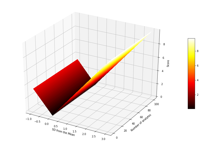
The behaviour of the numerical value is consistent through varying numbers of analytes and scales linearly with respect to deviation from the norm, and this graph explores the behaviour of the immune score over synthetically generated patient values as a function of number of analytes and divergence from healthy reference values.

Figure 3: The behaviour of NCCIS over synthetically generated patients with differing values and a deviation from the norm with respect to the respective expected values. The $x$ axis measures the stated analyte, while the $y$ axis measures the total number of analytes. In contrast to the behaviour of the immune score (Fig. 2), NCCISS is a non-linear function that displays a step-like behaviour by design, while remaining independent of the number of analytes.

Comparison	Sample Size (n)	p-value	F-value
Healthy vs Unhealthy	11976 vs 1107	P ¡ 0.0001	1011.03
Healthy vs Anemia	11976 vs 982	P ¡ 0.0001	900.89
Healthy vs HIV	11976 vs 62	P ¡ 0.0001	80.92
Healthy vs Hodgkin’s Disease	11976 vs 37	P ¡ 0.0001	17.95
Healthy vs Leukemia	11976 vs 18	P ¡ 0.0001	92.78
Healthy vs Blood Cancer	11976 vs 8	0.08029	3.06

Table 4: Differences in NIS Mean Values. All comparisons were performed using ANOVA.

Figure 4: Distribution of the Normalised Immune Score (NIS) from 0 to 10 ($y$ axis) among adult individuals in the NHANES 2000–2018 database.The Healthy cohort is defined as those individuals with all analytes within the normal ranges as defined by the NHS (1). Others comprise the Unhealthy set. After filtering for adult status (18 years old or older) and completeness of analyte information, a total of 53,114 individuals are represented in the plot.

Comparison	Sample Size (n)	p-value
Healthy vs Unhealthy	11976 vs 1107	P ¡ 0.0001
Healthy vs Anemia	11976 vs 982	P ¡ 0.0001
Healthy vs HIV	11976 vs 62	P ¡ 0.0001
Healthy vs Hodgkin’s Disease	11976 vs 37	P ¡ 0.0001
Healthy vs Leukemia	11976 vs 18	P ¡ 0.0001
Healthy vs Blood Cancer	11976 vs 8	P ¡ 0.0001

Table 5: Differences in NCCIS Mean Values. All comparisons were performed using ANOVA.

Figure 5: Distribution of the Normalised Colour-Coded Immune Score (NCCIS) from 0 to 10 ($y$ axis) among adult individuals in the NHANES 2000–2018 database. Individuals are defined as Healthy if all their analytes are within the normal ranges as defined by the NHS (1) and Unhealthy otherwise. After filtering for adult status (18 years old or older) and completeness of analyte information, a total of 53,114 individuals are represented in the plot. One explanation for the bimodality of some of these plots is the nature of the source data as self-reported where respondents may or may not have been ill at the time of giving their answers, or from the application of the separating cutoff value from NIS. In either case, both score separating capabilities are highly statistically significant.

In Table 6, we provide examples of CCIS and its correspondent NCCIS values for a sample of real-life and artificial cases. The second column of the table shows the NIS, for purposes of comparison. It is worth noting that these examples were generated using the NHS values for normal healthy subjects, and based on the provisional assumption that the distance between the upper and normal ranges is twice the standard deviation. The examples were taken from [8] as they were intended as very preliminary tests. We are aware that their source clearly states they are meant only for teaching purposes. Here they are used for purposes of illustration only, and the development of the NIS and NCCIS is not dependent on them.

One can observe how the NCCIS values meet the requirements we set in advance of their definition. We tested the NIS and NCCIS against real data from the National Health and Nutrition Examination Survey 2003–2016 (NHANES), provided in [28]. One measure of success was their ability to show how accurately the score discriminates between healthy subjects and patients suffering from various diagnosed illnesses.

To this end, we examined thousands of cases from [28] and calculated the distribution, mean values, and standard deviations for each of the analytes (see Fig. 7. We used the means and standard deviations from the data to define the metrics for both the NIS and NCCIS. Finally, we calculated the NIS and NCCIS for thousands of cases in the NHANES database to find individual scores. The resulting values were grouped as belonging to healthy individuals or to a selected list of common diseases.

In order to maximise the discriminatory power of both scores, we tried different alternative combinations of means, normal ranges and standard deviations, either taking these values from NHS values as of early 2022 or inferring them from the NHANES database (Fig. 7). At the end of the day, we settled for (1) NHS normal healthy reference values and means and standard deviations for the NIS; (2) means and standard deviations calculated from the NHANES database, and normal ranges from the NHS for the NCCIS. NHANES means and standard deviations are shown in Table 3.

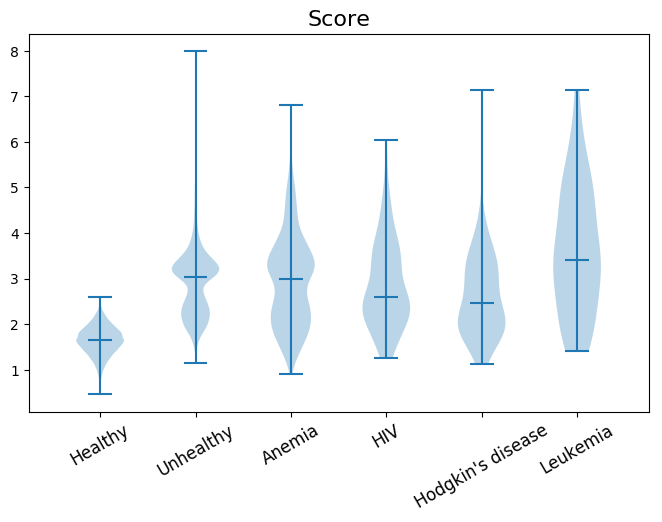
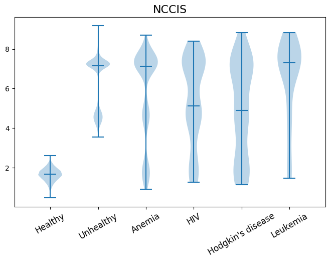
Figure 4 illustrates the distribution of NIS values across various (self-declared) conditions for individuals in the NHANES database. Table 4 presents the number of data points used, along with the respective ANOVA results to test statistical significance. It must be noted that the self-reported conditions were not independently confirmed. Moreover, the survey participants did not distinguish between current or past diagnoses. This could be expected to introduce some noise, as some currently healthy people will be labelled as having a condition and some people with conditions will not have been diagnosed. We hope to improve accuracy by filtering the data or by adding other data sources in the future.

Nevertheless, the NIS was able to discriminate between healthy and non-healthy individuals, as most healthy individuals are clustered around very low NIS values. In contrast, different conditions produced higher NIS values on average.

Conversely, the NCCIS did not substantially improve our knowledge of how some diseases impact analyte counts. There may be underlying co-morbidities or cases of blood-immune disorders that could create anomalous deviations from the predictions. Regardless, the methods are shown to be valid for predicting the complex immune profiles/trends (variation over time) observed in diverse patients when considering socio-clinical metadata parameters such as age, and sex, thereby suggesting their clinical applicability for purposes such as triaging and fast screening and extensions to such deviant clinical cases in prospective studies. In Fig. 5, it can be seen that reported medical conditions produce a higher average NCCIS value, but also induced some anomalous clustering, along with respective ANOVA analysis in table  5. Furthermore, the distribution of scores was even wider than that of the NIS. We thus concluded that the NCCIS did enhance the knowledge already gleaned from the NIS and the CCIS.

Table 6: Different tested scores perform differently according to each score’s definition.

Individual	NIS	CCIS	NCCIS
Adult male with all values at the mean	0.00	Green	0.00
Adult male values slightly removed from mean within normal healthy reference interval	1.84	Green	1.84
Adult male with all abnormal values	10.00	Red	10.00
Adult male with leukocytosis and diabetes	4.15	Red	7.60
Adult male with pancytopenia	5.54	Red	8.18
Adult male with mycosis	4.69	Red	7.83
Adult female with fatigue	3.07	Amber	5.43
Adult female with shortness of breath	6.70	Red	8.68
Adult female with thrombocytopenia	5.50	Red	8.16
Adult (female) with infection	3.63	Red	7.39

4.1 Linearisation and Separability

While the calculation of the score can incorporate normal ranges adjusted for age, race, sex, pregnancy stage, geography and any other consideration warranted by the literature, the score is intended to go beyond this clinical utility by capturing medical knowledge. A feature of the proposed (immune) score is the option to incorporate weights as multipliers in the form of scalars or piece-wise functions per analyte to modify its contribution relative to other analytes in a non-linear fashion, even under time sensitive conditions [11]. For example, in a blood differential test, conditions related to decreased white cell counts are milder than those associated with higher cell counts. However, the literature on conditions where there is a decrease of basophils, mast cells, monocytes and eosinophils in isolation is sparse, and reduced weights can be assigned to these possibly less-relevant markers.

Differences in cell shape and size, however, are usually more clinically significant and can be assigned greater weights. Typically, disorders affecting bone marrow function (i.e., blood cancers) result in the presence of abnormal (often immature) cells in peripheral blood; their presence in peripheral blood beyond this level would almost always be abnormal. A related point is whether the score can reflect subtle/minor changes in shape (variation in cell size, nuclear size, presence of other organelles) or only very crude and major deviations in size. For white blood cells, we do not yet understand what significance these have.

For example, the neutrophil-to-lymphocyte ratio relation is a key determinant of severity for sepsis, and involves 2 analytes. The synthetic analyte that can be added is the ratio itself, thus replacing a non-linear rule that would eventually make the score’s description too convoluted to read with ease with a key marker as another analyte [20, 25].

The scores introduced here are not intended to be used as a diagnostic tool on their own and can only quantify abnormality in terms of deviation from healthy reference (absolute or adaptable) values. The score is sensitive to out-of-range values and increases its value or changes its colour as a function of how removed values are from lower and upper bounds of reference values according to the number of standard deviations from the medians, but it cannot quantify diseases or conditions. The score indicates how far the bulk of all markers are from normal (healthy) reference values, the median, and an interval determined by published reference values for specific demographic or health conditions. Medians can be derived from empirical data (Fig. 6).

Figure 6: Distributions within ‘healthy’ reference values are heavily skewed in most cases, do not follow a normal or uniform distribution and often have long tails suggesting a personalised approach to reference values for abnormal results. The list of analyte labels is in the Supplementary Information.

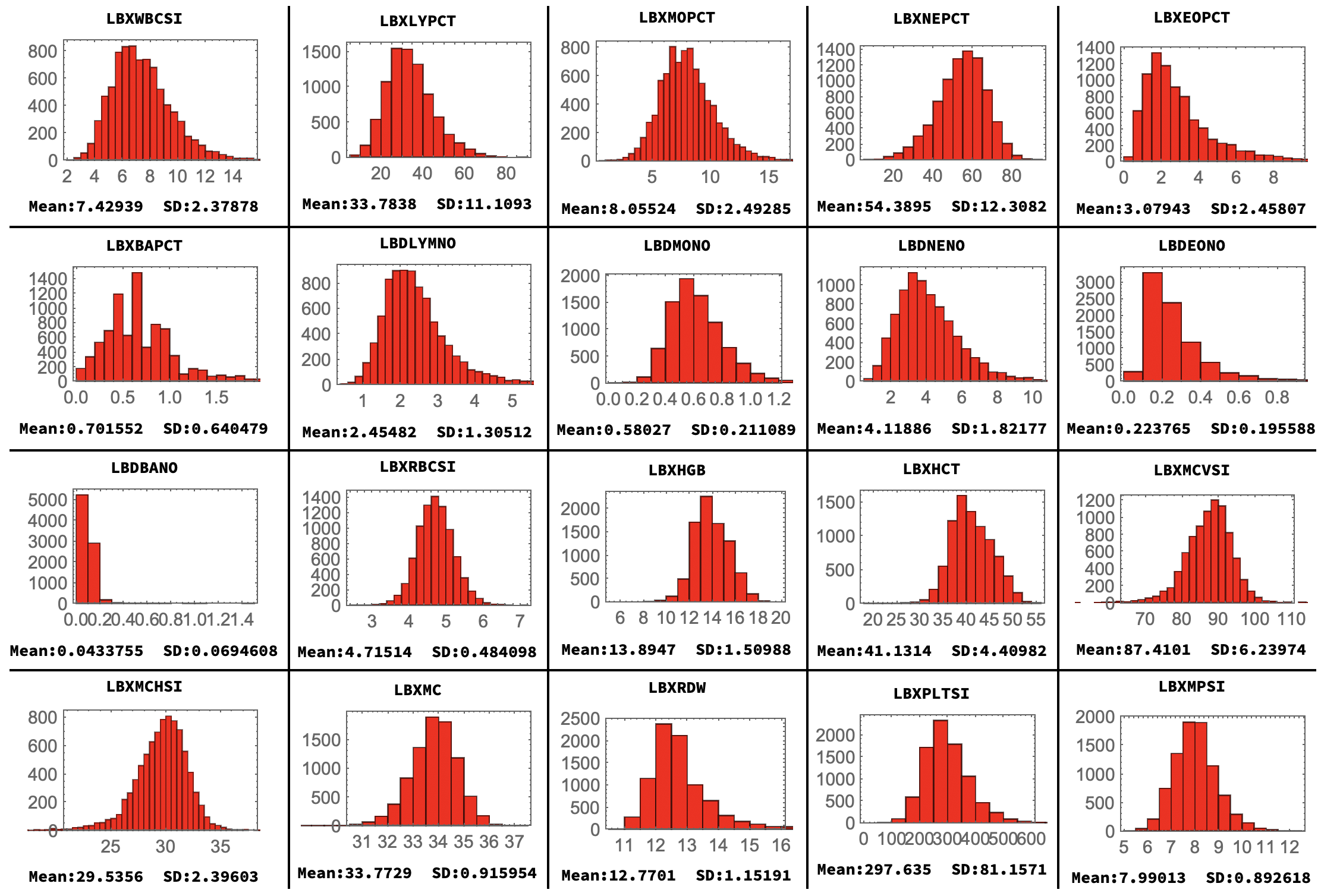
Figure 11 shows how male and female NHANES data can be distinguished by the scores using Red Blood Cell (RBC) counts as a health status predictor. The normal versus abnormal RBC ranges from the NHS were used to label the person as healthy or unhealthy. The Pearson $R^{2}$ value for RBC-dependent health status was found to be 0.176, for both sexes considered together. The Pearson $R^{2}$ values were 0.203 and 0.455, for male and female RBC counts considered separately, when comparing healthy and unhealthy groups.

We observed that the self-reported health status of the patients did not accurately predict their clinically assessed blood analytes. This was expected because self-reports may have reflected illness at various points in time in a person’s life rather than ongoing conditions. In other words, with this experiment, we de-noised the data by disregarding self-reported status to test the score against cleansed data based exclusively on CBC results as a discriminant, according to medical guidance on normal population reference values. That is, the interpretation of the health status a person could have potentially received from a medical doctor based exclusively on their CBC.

When healthy and unhealthy patients were separated using a subset of four CBC/FBC analyte measures, namely, MCH, HCT, neutrophil, and lymphocyte counts, as shown in Figure 13, we obtained the second best $R^{2}$ value of 0.075, for both sexes. The $R^{2}$values were 0.050 and 0.123, for the male and female groups, respectively. We found that neutrophil count alone, as a single clinical parameter, had a near equal performance as the composite measure of these four analyte parameters, with an $R^{2}$ of 0.072 when including both sexes. The inclusion of other white blood cell (WBC) parameters, such as monocyte count, eosinophil, and basophil, did not outperform these correlates. We observed that different subsets of a CBC/FBC by health status separated the data. All reported measures were statistically significant, with a two-tailed P$<0.0001$.

This also suggests that the mutlivariate biopsychosocial determinants of health should also be integrated for a top-bottom analysis of the disease predisposition and health dynamics of patients when assessing such self-reported measures. The irreducibility (multidimensionality) of these self-reported health measures may help explain why they are highly noisy and intersect with multiple other health factors, including multi-scale stressors such as the time of day, basic survival factors such as nutritional status/intake, sleep-related mood, psychological state, and social determinants of health, together with other health parameters.

4.2 Adaptive reference values

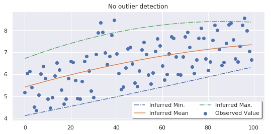
The reference ranges found in the medical literature are based on population-wide statistics that often fail to account for individual differences [6, 5]. To address this, we introduced an adaptive version of the immune score with the objective of providing personalised reference ranges to an individual’s medical history data. Our rationale is that, in applying the immune score to the resulting adaptive ranges, we obtain an immune score that is more significant in the statistical and clinical sense.

The main underlying assumption of this adaptive immune score definition is that, if a significant event (in the clinical sense) can be measured via an analyte, such an event will present itself as a value that breaks from the trend defined by the behaviour of the analyte over time. A second assumption is that such events can occur within the normal range as defined by a population reference range. A third assumption is that, while a trend becomes more incontrovertible the more data points there are, past values are less significant than proximate events. The next assumption is that the trend can be non-monotonous. The final assumption is that standard reference ranges can detect such events with acute sensitivity, while low specificity can thus be improved by narrowing the ranges but not by expanding them.

The adaptive feature of the immune score starts with a mathematical function that models the behaviour of an analyte as a time series (observed values over time). For each given point, the function assigns a linear approximation to the current and past data over a fixed time span (called a time step). The differential of this approximation is weighed against the differentials obtained for previous data via a linear combination of the current and previous derivatives. Finally, this linear approximation is evaluated over the mean time for the corresponding time-step. The resulting model is a function that carries the momentum of all previous values, and only previous values, yet remains adaptable for future long-term trends while being robust in the face of temporal disruptions to the trend. The speed of this adaptation can be controlled by hyper-parameters such as the size of the time step and the coefficients for the linear combination of differentials.

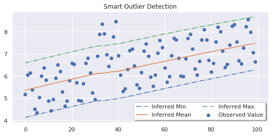
The function described in the preceding paragraph represents the adaptive mean, from which the adaptive ranges are inferred. The adaptive ranges consist of two functions, the upper limit and the lower limit. The upper limit is defined as the adaptive mean plus the standard deviation of all the values that are above the mean, up to the point of time in question. Similarly, the lower limit is the adaptive mean minus the standard deviation of all the values that are below the adaptive mean up to the relevant point in time. Next, we smooth the transition from the population ranges to the adaptive ranges by means of a linear combination of both ranges such that the adaptive range becomes the dominant factor in the time function.

Furthermore, this linear combination ensures that the adaptive ranges stay within the population ranges by defaulting to the population ranges whenever the resulting adaptive maximum is above the population maximum or the adaptive minimum is below the adaptive mean.

Figure 7: Statistical inference without smart outlier detection. In contrast to the smart outlier detection technology, simple statistical regression towards the observed values results in skewed inferred ranges.

Figure 8: Smart outlier detection example. The machine learning technology can adapt the range of expected values for all analytes, showing stable trends, while also detecting abnormal values or trends. In the image, we can show the result of machine learning inference of the ranges of normal values for a patient while also detecting abnormal values.

5 Immune age estimation

The immune system plays an important role in protecting against infections and in maintaining human health. Blood is the medium in which most immune cells circulate through the body.

Ageing is associated with complex changes and dysregulation of cellular processes. Nine tentative hallmarks that represent common denominators of ageing in different organisms have been described before[24].

As lifespan increases in many countries, there is a concomitant increase in age-related morbidities, particularly cardiovascular diseases, and increased susceptibility to seasonal infections, cancers, and neurodegenerative disorders. A unifying link between the higher rates of these disparate diseases observed in ageing populations is the progressive decline in immune functions.

It has been postulated that inflammation plays a critical role in regulating physiological ageing. Inflammatory components of the immune system are often chronically elevated in aged individuals, a phenomenon that has been termed “inflammageing” [12, 14, 13, 15, 17, 2].

However, the dynamics of this process at the individual level have not been characterised, hindering quantification of an individual’s ‘immune age’.

[2] used multiple ‘omics’ technologies to capture population- and individual-level changes in the human immune system in individuals of different ages sampled longitudinally over a nine-year period. They observed high inter-individual variability in the rates of change of cellular frequencies that was dictated by the individual’s baseline values, allowing identification of steady-state levels toward which a cell subset converged and the ordered convergence of multiple cell subsets toward older adult homeostasis.

In [16], an IMM-AGE score was described that captured an individual’s immune-ageing process. The IMM-AGE score correlated with age, yet it captured additional metrics such as cell-cytokine response better than chronological age.

Here we present a method where a single blood test, as in a complete full blood count of 13 blood analytes, gives insight into the immune age as compared to chronological age. Chronological age simply indicates the age of the individual, as determined by the length of time someone has lived or is living since their birth. This term should not be confused in the context of other literature, such as age estimates predicted by DNA methylation patterns from the Horvath algorithm.

5.1 Immune Score Over time

We hypothesised that as the human body ages the immune score will vary over time. In particular, we expected to see an upwards trajectory in direct relation to age.

To test the hypothesis, we selected two cohorts comprising all the data entries of individuals with ages ranging between 20 to 30 years, from the dataset, separating them by sex (male or female). These cohorts were used to build two immune spaces by computing the respective mean and standard deviations for each of the thirteen analytes. Afterward, for each sex, we selected seven cohorts of adults aged 20 to 25, 25 to 35, 35 to 45, 45 to 55, 55 to 65, 65 to 75, and 75 to 85 years of age, making for a total of 14 cohorts. Finally, we computed the immune score for each entry. The mean immune age for each of the cohorts is shown in Fig. 9.

(a)

(b)

Figure 9: (a) The mean immune age as a function of age for NHANES data. The reference ranges were computed over the population aged 20 to 90 for males and females, respectively. Each of the data points represents the mean immune score for the cohort $[age-5,age+5]$; for example, 50 represents the immune score for the population aged 45 to 55 years. (b)The distribution of immune age as a function of age. While a correlation trend is visible (especially for males), across sex the correlation is weak because healthy and non-healthy cohorts (both self-reported and by ground truth) are confounded.

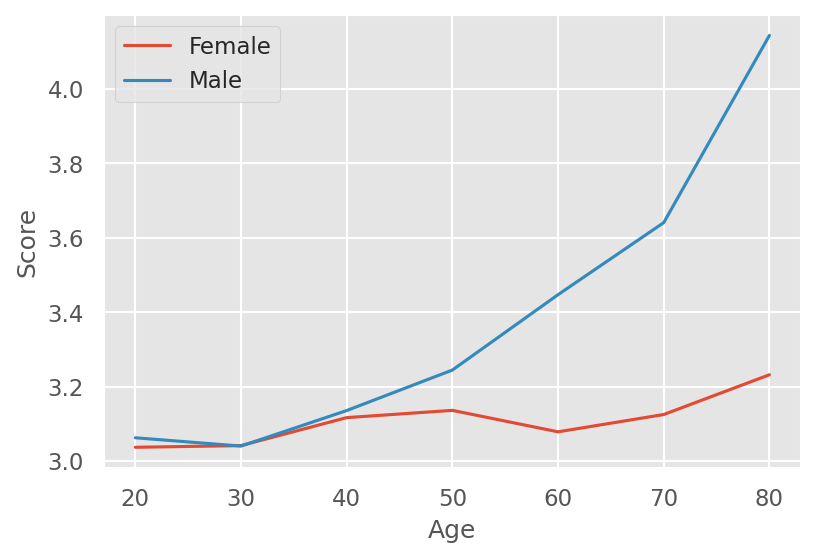
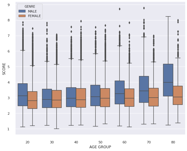
The results show significantly different behaviour over time for male and female cohorts. For subjects over the age of 30, it is evident that the male population presents an upward trajectory with respect to age for the mean immune score, as well as an increase in the 50th percentile and variance. However, the trend in females is slowed down (compared to males) between ages 40 and 50 and reversed between ages 50 and 60. It remains to be investigated whether some of the analytes involved are confounded with contradictory trends from other physiological differences, such as menopause, which occurs exactly between the ages where the slow-down and reversal in the age score trend for females is detected. It is known and has been reported that pregnancy and menopause produce a higher and more progressive increase in red cell counts, haematocrit levels and increased mean cell volume (MCV), and haemoglobin concentrations [21, 4, 9, 27, 1].

5.2 Immune age based on the immune score

We define the immune age as the reverse function of the relation between the expected immune score and the age of an individual. Formally:

Definition 5.1.

For a given immune score $\alpha$, the immune age $A:\alpha\mapsto a$ is defined as the function:

$$A(\alpha)=a.\overline{\{S(p):p\text{ age is }a\})}=\alpha,$$

where $\overline{\{S(p):p\text{ age is }a\})}$ is the mean immune score for all the individuals of age $a$.

In other words, the immune age is defined as the age in the function of the expected immune score; the immune age for a given score is the age cohort for which such a score is expected.

Given the observed behaviour of the mean immune score over time, we assert that we can apply the given immune age definition for males aged 20 or older. However, we have shown that the functional relation is much weaker, or nonexistent, in the female population.

As explained in Section 5.1, the data compiled comprises a list of seven values representing the mean immune score for each of the seven age cohorts. In order to apply the Definition 5.1, we fitted a linear model of degree 3 to the data, obtaining a monotonously decreasing function that allows us to interpolate and extrapolate the expected immune score over specific ages. The resulting curve, which we call an immune age curve, is shown in Fig. 10.

Figure 10: A linear approximation of degree 3 to the mean score over seven age cohorts from the healthy groups only. The linear model smooths the curve and allows for extrapolation.

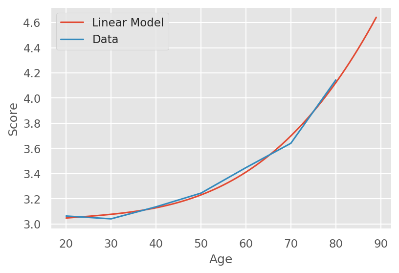
We will only consider integer ages in years. Therefore we can represent the immune age curve by a list of 70 real values that contains the inferred immune score for each age between 20 and 90. Let us denote this curve by the list of pairs $\text{IAC}=\langle(20,3.0),(21,3.1),\dots,(a,\alpha),\dots,(90,4.75)\rangle$.

We now can obtain the immune age $A$ by means of the following function:

$$A(\alpha)=\begin{cases}20\quad&\text{if}\,\alpha\leq 3\\ 90\quad&\text{if}\,\alpha\geq 4.75\\ a.(a,\alpha^{*})\in\text{IAC}\quad&\text{elsewhere}\end{cases}$$

where $\alpha^{*}$ is the closest score in $IAC$ to $\alpha$. If there are two scores at the same distance, we choose the leftmost option. The resulting function is shown in Fig. 13. The curve shows some minor bumps which are the results of the discretisation used. We maintain that this distortion is not significant.

As a tool that returns an estimated age with respect to a score, we can analyse its predictive power. Using the NHANES data and focusing on males aged 20 to 90, we can measure the error of using the score to predict a person’s age.

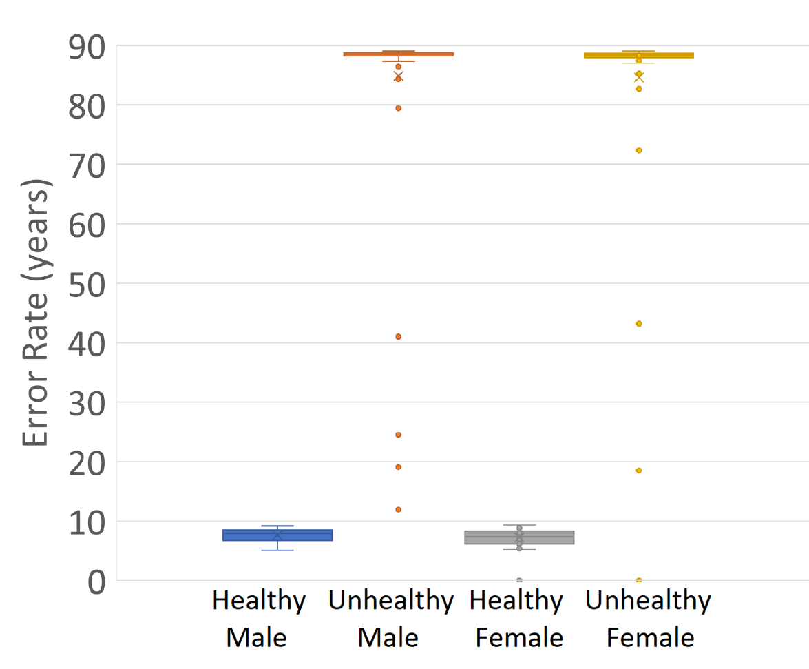
As shown in Figure 14, prediction error rates are much lower in healthy NHANES data, compared to unhealthy groups, for both sexes and therefore can be used to estimate the chronological age of healthy patients. Prediction error rates for the immune score age were overestimated by approximately 7 years, for the healthy groups, in both sexes, allowing a correction (mean error rate of 7.33 $\pm$ 1.21 for healthy females, and 7.62 $\pm$ 1.17 for healthy males). Furthermore, there is a statistically significant difference between the healthy and non-healthy groups (regardless of sex) in the error rates of age prediction. Pearson’s correlation statistics on the age error rates predicted, by the health status of the red blood cell count, as discussed before, were an R square value of 0.293 and 0.168, for men (P$<$ 0.0001) and females (P$<$0.013). Age prediction error rates were high and not significant when self-reported health measures were used to separate health status groups, but were significant when taking abnormal CBC values only.

Table 7: Statistics of each CBC analyte as a predictor or discriminant of health and age.

Counts	Healthy	Unhealthy	Age
BASO	0.0051	0.0166	0.0004
EOS	0.0012	2.00E-05	0.0049
HCT	0.0036	0.0055	0.0696
HGB	0.1179	0.1397	0.0635
LYMP	0.0429	0.4983	0.0928
MCH	0.0831	0.0001	0.1538
MCHC	0.0025	0.0043	0.0047
MCV	0.2661	0.337	0.2186
MONO	0.0121	0.0004	0.0073
NEUT	0.0084	0.0069	0.018
RBC	0.0268	1.00E-05	0.0009
PLT	0.0921	0.3334	0.1029

Table 7 shows the statistics of the predictors and separators of age for healthy and unhealthy populations. These plots show that common blood marker dynamics are predictive of age and health.

There are small but potentially meaningful differences between reference ranges. This could affect the classification of out-of-range counts when applying mismatched country-specific ranges. Using uniform, population-appropriate references is important for generalizable models but our main contribution is to learn each individual personal reference values hence making the reference discrepancies per country less relevant.

Table 8: Best predictors for each category

Healthy	Unhealthy	Age
MCV	LYMP	MCV
HGB	MCV	MCH
PLT	PLT	PLT
MCH	HGB	LYMP
LYMP	BASO	HCT
RBC	NEUT	HGB
MONO	HCT	NEUT
NEUT	MCHC	MONO
BASO	MONO	EOS
HCT	MCH	MCHC
MCHC	EOS	RBC
EOS	RBC	BASO

Figure 11: Age Prediction Error Rates between actual patient (biological) age and Immune-score predicted age from NHANES dataset by RBC counts. The health status was determined by the best blood analyte correlate in this case, as previously discussed, the RBC counts, to separate healthy from unhealthy groups by sex. The results show that the immune-score predicted age has the lowest prediction error rate among healthy groups, for both sexes and overestimates age when the individuals are not healthy.

6 Conclusion

We have introduced risk-assessment scores and studied their behaviour against typical synthetic and empirical disease cases. We have introduced a learning procedure to adapt normal versus abnormal reference values to personalised ranges for more precise and individual medical assessment and demonstrated the capabilities and applications of the scores for triaging purposes against a popular public database showing how the scores separate healthy from unhealthy cohorts both self-reported with significant noise and determined by typical normal reference values. The approaches were shown to be informative for quick and entry-level patient health sorting and triaging.

The numerical score was shown to be able to define an ‘immune age’, with some differences for males and females who are known to show greater fluctuations due to e.g. menopause. In the case of estimation of immune age, the chronological age of healthy people was closely predicted by common hematological markers typically measured in FBC or CBC, and for unhealthy self-reported or by typical abnormal reference values, the score was not predictive of chronological age, conforming with the theoretical expectation of a good predictor of health by the divergence between estimated immune and actual chronological age.

Unlike statistical or traditional machine learning and black-box approaches, the approach introduced is transparent to clinicians, health professionals, and health consumers who can follow the calculations and interpretation to be assessed in a clinical context for rapid screening and decision support.

Appendix

Table 9: List of blood-related label headers in the NHANES database

LBXWBCSI	White blood cell count (1000 cells/uL)
LBXLYPCT	Lymphocyte percent (%)
LBXMOPCT	Monocyte percent (%)
LBXNEPCT	Segmented neutrophils percent (%)
LBXEOPCT	Eosinophils percent (%)
LBXBAPCT	Basophils percent (%)
LBDLYMNO	Lymphocyte number
LBDMONO	Monocyte number
LBDNENO	Segmented neutrophils number
LBDEONO	Eosinophils number
LBDBANO	Basophils number
LBXRBCSI	Red blood cell count (million cells/uL)
LBXHGB	Haemoglobin (g/dL)
LBXHCT	Haematocrit (%)
LBXMCVSI	Mean cell volume (fL)
LBXMCHSI	Mean cell haemoglobin (pg)
LBXMC	MCHC (g/dL)
LBXRDW	Red cell distribution width (%)
LBXPLTSI	Platelet count SI (1000 cells/uL)
LBXMPSI	Mean platelet volume (fL)

Data

The National Health and Nutrition Examination Survey[28] is a research program conducted by the National Center for Health Statistics (NCHS) of the United States of America. This program offers a public database that contains information relating to the demographic, health, and nutritional status of adults and children in the USA. In particular, it offers individual laboratory results for the thirteen analytes, along with demographic information (such as age, biological sex, among others) for thousands of individuals collected over 20 years.

For the immune age sections, we extracted a subset of 31900 individuals chosen according to the following criteria.

• 20 years of age or older as stated by RIDAGEYR.

• The general health condition (all self-reported) variable (HSD010) was stated as Good, Very Good or Excellent.

• The values for the 13 analytes, along with the general health condition, age and sex (RIAGENDR) were present in the data.

References

- [1] José M Aldrighi et al. “Platelet activation status decreases after menopause” In Gynecol Endocrinol 20.5, 2005, pp. 249–57 DOI: 10.1080/09513590500097549.
- [2] Ayelet Alpert et al. “A clinically meaningful metric of immune age derived from high-dimensional longitudinal monitoring” In Nat Med 25.3, 2019, pp. 487–495 DOI: 10.1038/s41591-019-0381-y.
- [3] Jeffrey L Anderson et al. “Usefulness of a complete blood count-derived risk score to predict incident mortality in patients with suspected cardiovascular disease” In Am J Cardiol. 99.2, 2007, pp. 169–74 DOI: 10.1016/j.amjcard.
- [4] John Aneke et al. “Changes in Haematological Indices of Women at Different Fertility Periods in Nnewi, South-East, Nigeria” In J Med Res 2, 2016, pp. 166–169 DOI: 10.31254/jmr.2016.2610
- [5] Petter Brodin and Mark M Davis “Human immune system variation” In Nat Rev Immunol. 17.1, 2017, pp. 21–29 DOI: 10.1038/nri.2016.125.
- [6] Petter Brodin et al. “Variation in the human immune system is largely driven by non-heritable influences” In Cell 160.1-2, 2015, pp. 37–47 DOI: 10.1016/j.cell.2014.12.020.
- [7] “Case Index by Patient History” In NHS Foundation Trust, York Teaching Hospital URL: https://www.yorkhospitals.nhs.uk/seecmsfile/?id=2396
- [8] “Case Index by Patient History” In University of Pittsburgh, Department of Pathology, 2022, pp. Accessed on URL: https://path.upmc.edu/cases/
- [9] J.. Cruickshank “Some Variations in the Normal Haemoglobin Concentration” In British Journal of Haematology 18.5, 1970, pp. 523–530 DOI: https://doi.org/10.1111/j.1365-2141.1970.tb00773.x
- [10] F H Edwards et al. “The Society of Thoracic Surgeons National Cardiac Surgery Database: current risk assessment” In Ann Thorac Surg. 63.3, 1997, pp. 903–8 DOI: 10.1016/s0003-4975(97)00017-9.
- [11] I. Erdemir “The comparison of blood parameters between morning and evening exercise” In European Journal of Experimental Biology 3.1, 2013, pp. 559–563
- [12] C Franceschi et al. “Inflamm-aging. An evolutionary perspective on immunosenescence” In Ann N Y Acad Sci. 908, 2000, pp. 244–54 DOI: 10.1111/j.1749-6632.2000.tb06651.x.
- [13] Claudio Franceschi and Judith Campisi “Chronic inflammation (inflammaging) and its potential contribution to age-associated diseases” In J Gerontol A Biol Sci Med Sci. 69.1, 2014, pp. 4–9 DOI: 10.1093/gerona/glu057.
- [14] Claudio Franceschi et al. “Inflammaging and anti-inflammaging: a systemic perspective on aging and longevity emerged from studies in humans” In Mech Ageing Dev. 128.1, 2006, pp. 92–105 DOI: 10.1016/j.mad.2006.11.016.
- [15] Claudio Franceschi et al. “Inflammaging and ’Garb-aging”’ In Trends Endocrinol Metab 28.3, 2017, pp. 199–212 DOI: 10.1016/j.tem.2016.09.005.
- [16] David Furman et al. “Chronic inflammation in the etiology of disease across the life span” In Nat Med 25.12, 2019, pp. 1822–1832 DOI: 10.1038/s41591-019-0675-0.
- [17] David Furman et al. “Expression of specific inflammasome gene modules stratifies older individuals into two extreme clinical and immunological states” In Nat Med 23.2, 2017, pp. 174–184 DOI: 10.1038/nm.4267.
- [18] Benjamin D Horne et al. “Complete blood count risk score and its components, including RDW, are associated with mortality in the JUPITER trial” In Eur J Prev Cardiol. 22.4, 2014, pp. 519–26 DOI: 10.1177/2047487313519347.
- [19] Benjamin D Horne et al. “The Intermountain Risk Score (including the red cell distribution width) predicts heart failure and other morbidity endpoints” In Eur J Heart Fail 12.11, 2010, pp. 1203–13
- [20] R. Kaushik et al. “Diagnostic and Prognostic Role of Neutrophil-to-Lymphocyte Ratio in Early and Late Phase of Sepsis” In Indian J Crit Care Med. 22.9, 2018, pp. 660–663 URL: https://www.ncbi.nlm.nih.gov/pmc/articles/PMC6161585/
- [21] Vuokko Kovanen et al. “Design and protocol of Estrogenic Regulation of Muscle Apoptosis (ERMA) study with 47 to 55-year-old women’s cohort: novel results show menopause-related differences in blood count” In Menopause 25.9, 2018, pp. 1020–1032 DOI: 10.1097/GME.0000000000001117.
- [22] Michael Kristensen et al. “Routine blood tests are associated with short term mortality and can improve emergency department triage: a cohort study of patients” In Scand J Trauma Resusc Emerg Med. 25.1, 2017, pp. 115 DOI: 10.1186/s13049-017-0458-x.
- [23] Lawrence Liao et al. “A new anatomic score for prognosis after cardiac catheterization in patients with previous bypass surgery” In J Am Coll Cardiol. 46.9, 2005, pp. 1684–92 DOI: 10.1016/j.jacc.2005.06.074.
- [24] Carlos López-Otín et al. “The Hallmarks of Aging” In Cell 153.6, 2013, pp. 1194–217 DOI: 10.1016/j.cell.2013.05.039
- [25] E.. Martins et al. “Neutrophil-lymphocyte ratio in the early diagnosis of sepsis in an intensive care unit: a case-control study” In Rev Bras Ter Intensiva. 31.1, 2019, pp. 63–70 URL: https://www.ncbi.nlm.nih.gov/pmc/articles/PMC6443306/#:~:targetText=The%5C%20presence%5C%20of%5C%20a%5C%20neutrophil,were%5C%20related%5C%20to%5C%20patient%5C%20mortality.
- [26] Omid Fatemi Mohammad Madjid “Components of the complete blood count as risk predictors for coronary heart disease: in-depth review and update” In Tex Heart Inst J. 40.1, 2013, pp. 17–29
- [27] Daisuke Nakada et al. “Estrogen increases haematopoietic stem-cell self-renewal in females and during pregnancy” In Nature 505.7484, 2014, pp. 555–558 DOI: 10.1038/nature12932
- [28] “National Health and Nutrition Examination Survey” In Centers for Disease Control and Prevention, National Center for Health Statistics, 2016 URL: https://wwwn.cdc.gov/nchs/nhanes/Default.aspx
- [29] Xiaowei Niu et al. “Risk stratification based on components of the complete blood count in patients with acute coronary syndrome: A classification and regression tree analysis” In Sci Rep. 8.1, 2018, pp. 2838 DOI: 10.1038/s41598-018-21139-w.
- [30] Quinn R Pack et al. “Development and Validation of a Predictive Model for Short- and Medium-Term Hospital Readmission Following Heart Valve Surgery” In J Am Heart Assoc. 5.9, 2016 DOI: 10.1161/JAHA.116.003544.
- [31] I Ringqvist et al. “Prognostic value of angiographic indices of coronary artery disease from the Coronary Artery Surgery Study (CASS)” In J Clin Invest. 71.6, 1983, pp. 1854–66 DOI: 10.1172/jci110941.
- [32] P W Wilson et al. “Prediction of coronary heart disease using risk factor categories” In Circulation 97.18, 1998, pp. 1837–47 DOI: 10.1161/01.cir.97.18.1837.
- [33] Jack E Zimmerman, Andrew A Kramer, Douglas S McNair and Fern M Malila “Acute Physiology and Chronic Health Evaluation (APACHE) IV: hospital mortality assessment for today’s critically ill patients” In Crit Care Med. 34.5, 2006, pp. 1297–310 DOI: 10.1097/01.CCM.0000215112.84523.F0.
- [34] Ming-Xiang Zou et al. “A four-factor immune risk score signature predicts the clinical outcome of patients with spinal chordoma” In Clin Transl Med. 10.1, 2020, pp. 224–237 DOI: 10.1002/ctm2.4.