Cooperative Data Collection with Multiple UAVs for Information Freshness in the Internet of Things

Abstract

Maintaining the freshness of information in the Internet of Things (IoT) is a critical yet challenging problem. In this paper, we study cooperative data collection using multiple Unmanned Aerial Vehicles (UAVs) with the objective of minimizing the total average Age of Information (AoI). We consider various constraints of the UAVs, including kinematic, energy, trajectory, and collision avoidance, in order to optimize the data collection process. Specifically, each UAV, which has limited on-board energy, takes off from its initial location and flies over sensor nodes to collect update packets in cooperation with the other UAVs. The UAVs must land at their final destinations with non-negative residual energy after the specified time duration to ensure they have enough energy to complete their missions. It is crucial to design the trajectories of the UAVs and the transmission scheduling of the sensor nodes to enhance information freshness. We model the multi-UAV data collection problem as a Decentralized Partially Observable Markov Decision Process (Dec-POMDP), as each UAV is unaware of the dynamics of the environment and can only observe a part of the sensors. To address the challenges of this problem, we propose a multi-agent Deep Reinforcement Learning (DRL)-based algorithm with centralized learning and decentralized execution. In addition to the reward shaping, we use action masks to filter out invalid actions and ensure that the constraints are met. Simulation results demonstrate that the proposed algorithms can significantly reduce the total average AoI compared to the baseline algorithms, and the use of the action mask method can improve the convergence speed of the proposed algorithm.

I Introduction

There is a rising need to support ubiquitous connections for Internet of Things (IoT)-based applications, such as monitoring agricultural growth, tracking marine life, and surveilling border areas, to name but a few, in remote geographical areas where terrestrial network infrastructures are limited. To meet this need, Unmanned Aerial Vehicles (UAVs) have emerged as a promising technology for providing timely, flexible, and elastic services in underserved areas due to their high mobility and agility [2][3]. Specifically, UAVs equipped with microprocessors and wireless transceivers can dynamically move towards each sensor in IoT networks to collect or disseminate information. With their fully controllable mobility and high altitude, UAVs can exploit the Line-of-Sight (LoS) wireless communications on the air-to-ground channel to improve throughput and reduce transmission energy consumption. Moreover, UAVs can be dispatched on demand and their locations can be promptly adjusted according to the dynamic communication environment, providing fast and flexible reconfiguration.

Due to their attractive characteristics, UAV-enabled IoT networks have gained considerable attention and aroused numerous research interests in recent years. However, most of the existing works have focused on optimizing traditional performance metrics, such as system throughput, coverage, and delay [4, 5, 6, 7, 8]. These performance metrics fail to quantify the freshness of information in the UAV-enabled IoT networks, which is critical for mission-critical applications [9, 10], such as forest fire containment and extinguishment, and disaster relief surveillance and rescue. In these applications, the accuracy of the decisions made using the collected information from IoT devices depends heavily on the freshness of the information. This has led to the use of the Age of Information (AoI) as a measure of fresh information from the receiver’s perspective [11, 12, 13].

Due to the limited onboard energy of the UAV, it is difficult, if not impossible, to collect data from all the sensors in a large area within a stringent time requirement using a single UAV. Therefore, it is necessary to study cooperative data collection with multiple UAVs. However, compared with the single UAV-enabled IoT networks, there are several technical challenges that result from having multiple UAVs. Firstly, since the UAVs would collide with each other, the additional collision avoidance constraint has to be guaranteed when designing the UAVs’ trajectories. Secondly, due to the mutual interference among the simultaneous status updating, the scheduling of the IoT device has to be carefully designed as well to mitigate transmission failure. Thirdly, since the dynamic of the environment is affected by the actions of all UAVs, the environment faced by each UAV is non-stationary. Lastly, the action space increases exponentially with the number of UAVs, making it more difficult to find an optimal decision. Previous studies in this area have relied on global state information for coordination [14, 15], which can lead to significant communication overhead. Therefore, further study is needed on how to cooperatively collect status update packets from sensors with multiple UAVs in a decentralized manner in order to maintain information freshness.

Motivated by these facts, we consider the IoT networks without terrestrial network infrastructures and investigate the problem of cooperative data collection with multiple UAVs for information freshness. In this model, each UAV acts as an individual agent. Specifically, each UAV with a limited amount of onboard energy is dispatched from its depot, flies towards the sensors to collect status update packets, and finally arrives at the destination within a fixed period. These UAVs must avoid collisions during the flight and reach their destinations before running out of energy. Each sensor node is equipped with a battery and can harvest energy from the ambient environment. The sensor is only available when it has enough energy. We jointly design the trajectories of UAVs and the scheduling of sensors to minimize the total average AoI. The main contributions of this paper are summarized as follows.

• We formulate the multi-UAV data collection problem as a finite-horizon Decentralized Partially Observable Markov Decision Process (Dec-POMDP) due to the lack of terrestrial network infrastructures, the limited observation of each UAV, and the unknown dynamics of the environment, including the energy harvesting rate of the sensors and the line-of-sight probability of the air-to-ground channel.

• We propose a multi-agent deep reinforcement learning (DRL) based algorithm with Centralized Training with Decentralized Execution (CTDE) to cope with the non-stationary environment. Particularly, the UAVs are jointly trained by leveraging global information in the training phase, whereas each UAV makes the decision independently based on its own observation in the execution phase. Moreover, to ensure the kinematic, energy, and trajectory constraints, we use an action mask to filter out the invalid actions during the training and execution phases.

• We conduct extensive simulations to evaluate the performance of the proposed algorithm. The results show that the proposed algorithm can effectively coordinate the trajectories of UAVs and the scheduling of sensors. Compared with the baseline algorithms, the total average AoI of the proposed algorithm is significantly reduced.

The paper is organized as follows: The related work is summarized in Section II. The system model and problem formulation are described in Section III. The multi-agent DRL approach is proposed in Section IV. The simulation results and discussions are given in Section V. Finally, we conclude this paper in Section VI.

II Related Work

II-A Single-UAV Data Collection

The collection of fresh data in IoT networks using a single unmanned aerial vehicle (UAV) has been extensively studied. In [16], the UAV’s flight trajectory was designed to minimize the number of expired packets based on Q-learning, taking into account the AoI deadline constraint imposed on each sensor. In [17], two age-optimal data collection problems were formulated to minimize either the average AoI or peak AoI, where the sensors are grouped into non-overlapping clusters and the UAV flies along with the collection points to collect data from a set of sensors. Both the charging time and trajectory of the UAV were designed to minimize the average AoI for UAV-assisted wirelessly powered IoT networks in [18], where the UAV charges the sensors before collecting state updates from them. In [19], considering three data acquisition strategies of UAV, i.e., hovering, flying, and hybrid, a dynamic programming algorithm was used to optimize the visiting order of the SNs and data acquisition strategies to minimize the average AoI while also satisfying the energy constraints of the SN. The above studies [16, 17, 18, 19] all involve the UAV collecting status update packets from each sensor only once, whereas in [20, 21], the UAV is allowed to visit each sensor multiple times within a given time period. A DRL algorithm was proposed to optimize the UAV’s trajectory and the scheduling of sensors with the objective of minimizing the normalized weighted sum of AoI in [20], and this was extended in [21] by combining DRL and convex optimization.

However, the energy consumption of the UAV has been ignored in these previous works. In reality, it is important to consider the UAV’s energy consumption when designing its flight trajectory due to the limited onboard battery of the UAV. In our earlier work [1], the age-optimal flight trajectory and transmission scheduling were jointly designed considering both the energy and time constraints. In [22], the UAV was used as a mobile relay and the average PAoI was minimized by jointly optimizing the UAV’s flight trajectory, energy allocations, and transmission time durations at both the sensor and the UAV. In [23], the sensing and communication trade-off was studied in terms of time and energy consumption for the cellularly connected UAV. In [24], the UAV’s flight speed, hovering locations, and bandwidth allocation were jointly optimized to minimize the weighted sum of the expected average AoI, propulsion energy of the UAV, and the transmission energy at IoT devices.

II-B Multi-UAV Data Collection

There have been several studies that involve the use of multiple UAVs for collaborative data collection. In one study [25], UAVs were used to collect data generated by vehicles in intelligent transportation systems and the Deep Deterministic Policy Gradient (DDPG) algorithm was used to optimize the UAVs’ trajectories and the transmission scheduling of vehicles in order to minimize the expected weighted sum AoI. Another study [26] utilized the Deep Q-Network (DQN) to design the cooperative trajectories of the UAVs in order to maximize total energy efficiency under both energy and AoI constraints. While these studies both involve multiple UAVs, all of the UAVs’ actions are controlled by a single agent, which can result in a very large action space.

In contrast, the study [14] proposed a distributed sense-and-send protocol in which each UAV acts as its own agent and makes its own decisions based on a compound action actor-critic algorithm in order to minimize the AoI. This approach was further extended in [15], where a multi-UAV trajectory design algorithm based on DDPG was proposed to minimize the AoI for UAV-to-device communications. However, in these studies, each UAV must communicate with the BS in order to obtain the full knowledge of all other UAVs’ states, leading to significant signaling overhead.

In [27], two UAVs were used, one as an energy transmitter and the other as a data collector, and the Independent DQN (IDQN) algorithm was employed to design the UAVs’ trajectories in order to minimize the AoI, enhance energy transfer to devices, and minimize UAV energy consumption. With IDQN, each UAV makes decisions based on its own observations, but the convergence of IDQN is not guaranteed in a non-stationary multi-agent environment. To address this issue, we model the collaborative data collection problem as a Dec-POMDP and adopt the CTDE framework in this work. Specifically, multiple UAVs are centrally trained with global state information to ensure convergence, and then each UAV makes its decisions based on local observations without the need for a central entity to collect and disseminate global state information.

III System Model and Problem Formulation

In this section, we first describe the multi-UAV enabled IoT network. Then, we present the energy consumption model, the air-to-ground channel model, and the evolution of the age of information. Finally, we formulate a data collection problem by optimizing the flight trajectories of the UAVs and the transmission scheduling of the sensors.

III-A Scenario Description

As shown in Fig. 1, we consider a multi-UAV enabled IoT network containing $N$ randomly distributed sensor nodes (SNs). The set of all SNs is denoted by $\mathcal{N}=\{1,2,\ldots,N\}$ and the location of SN $n\in\mathcal{N}$ is represented by $\bm{w}_{n}=(x_{n},y_{n},0)$ in a three-dimensional Cartesian coordinate system. A swarm of $M$ rotary-wing UAVs is employed to cooperatively collect status updates from the SNs, which are directly used by the UAVs to execute certain tasks. The set of all UAVs is denoted as $\mathcal{M}=\{1,2,\ldots,M\}$. We assume a discrete-time system where time is divided into equal-length time slots, each lasting $\tau_{0}$ seconds. The UAVs are required to support collaborative data collection for a total of $T$ time slots. In particular, UAV $m\,(m\in\mathcal{M})$ takes off from an initial location $\boldsymbol{u}_{m}^{\text{start}}$ and flies over various SNs to collect their status updates. By the end of the $T$-th slot, the UAV needs to arrive at its final destination $\boldsymbol{u}_{m}^{\text{stop}}$.

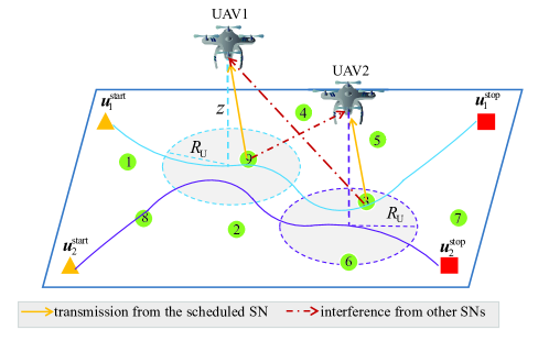
Figure 1: An illustration of multi-UAV enabled data collection.

At the beginning of time slot $t$, the location of UAV $m\in\mathcal{M}$ in the three-dimensional Cartesian coordinate is denoted by $\boldsymbol{u}_{m}(t)=(x_{m}(t),y_{m}(t),z_{m}(t))$, where $(x_{m}(t),y_{m}(t))$ is the projection of the location of UAV $m$ on the ground and $z_{m}(t)$ is the altitude of UAV $m$. We assume that all UAVs fly at the same fixed altitude, i.e., $z_{m}(t)=z,\forall t$. The velocity of UAV $m$ at the beginning of time slot $t$ is represented in polar coordinates and denoted by $\boldsymbol{v}_{m}(t)=(v_{m}^{s}(t),\varphi_{m}(t))$, where $v_{m}^{s}(t)=\left\|\boldsymbol{v}_{m}(t)\right\|$ is the speed of UAV $m$ and $\varphi_{m}(t)$ is the velocity direction with $0\leq\varphi_{m}(t)\leq 2\pi$. We assume a constant acceleration $\bm{a}_{c,m}(t)=\dot{\bm{v}}_{m}(t)$ during one time slot and hence the velocity can be updated by $\bm{v}_{m}(t+1)=\bm{v}_{m}(t)+\bm{a}_{c,m}(t)\tau_{0}$. As the quad-rotor UAV is able to easily steer by adjusting the rotation rate of four rotors, we assume that the UAV can change its direction instantly at the beginning of a time slot, and the flight direction is then fixed for the rest of the time slot. In practice, UAVs are subject to kinematic constraints. In particular, the speed of the UAV $m$ at the slot $t$ cannot exceed its maximum value $v_{\max}^{s}$, i.e., $v_{m}^{s}(t)\leq v_{\max}^{s}$, and the turning angle of UAV $m$ at the slot $t$, $\triangle\varphi_{m}(t)=\varphi_{m}(t)-\varphi_{m}(t-1)$, cannot exceed its maximum value $\triangle\varphi_{\max}$, i.e., $\mid\triangle\varphi_{m}(t)\mid\leq\triangle\varphi_{\max}$. We denote the velocities of all UAVs as $\boldsymbol{V}=(\bm{v}_{1},\bm{v}_{2},\ldots,\bm{v}_{M})$, where $\bm{v}_{m}=(\boldsymbol{v}_{m}(1),\boldsymbol{v}_{m}(2),\ldots,\boldsymbol{v}_{m}(T))$ represents the sequence of velocities of UAV $m$. The flight trajectory of UAV $m$ is defined as a sequence of locations it flies over, i.e., $\bm{p}_{m}=(\bm{u}_{m}(1),\bm{u}_{m}(2),\ldots,\boldsymbol{u}_{m}(T))$, where $\bm{u}_{m}(1)=\bm{u}_{m}^{\text{start}}$ and $\bm{u}_{m}(T)=\bm{u}_{m}^{\textrm{stop}}$. To avoid collisions between the UAVs, the distance between any two UAVs at time slot $t$ cannot be less than the safe distance, i.e., $d_{m,m^{\prime}}(t)\geq d_{\textrm{safe}}$, for any $m\neq m^{\prime}(m,m^{\prime}\in\mathcal{M})$.

Each UAV has a coverage area on the ground with radius $R_{U},m\in\mathcal{M}$, which is fixed and determined by the transmit power of the SN, the altitude of the UAV, the antenna gains, and the channel path loss. In particular, we set the radius as $R_{U}=\sqrt{d^{2}-z^{2}},$ where $d=\frac{c}{4\pi f_{c}}\left(\frac{P_{c}G_{s}G_{u}}{\xi_{\text{th}}\sigma^{2}\eta_{\text{NLoS}}}\right)^{1/\varsigma}$. The specific notations will be explained in Subsection III-C. Let $\overline{d}_{n,m}(t)$ denote the distance between SN $n$ and the projection of UAV $m$ on the ground at the beginning of slot $t$. If $\overline{d}_{n,m}(t)\leq R_{U}$, then SN $n$ is within the coverage area of UAV $m$ at slot $t$. At every time slot, each UAV has to decide which SN within its coverage area is scheduled to update its status. Let $\boldsymbol{b}_{m}=(b_{m}(1),b_{m}(2),\ldots,b_{m}(T))$ be the SN scheduling vector of UAV $m$, where $b_{m}(t)=n$ indicates that SN $n$ transmits a status update packet to UAV $m$ at time slot $t$ and $b_{m}(t)=0$ means that no SN is scheduled by UAV $m$ at time slot $t$. The SN scheduling vector of all UAVs is represented by $\boldsymbol{B}=(\boldsymbol{b}_{1},\boldsymbol{b}_{2},\ldots,\boldsymbol{b}_{M})$.

III-B Energy Model

III-B1 UAV Energy Model

We assume that all the UAVs have the same amount of initial onboard energy, denoted by $E_{\text{max}}$. The major energy consumption of the UAV consists of communication energy and propulsion energy. Since each UAV acts as a receiver for the status update packets, its communication energy consumption is much smaller than the propulsion energy consumption and hence can be ignored. The propulsion energy consumption of UAV $m$ $E_{m}(t)$ in time slot $t$ can be expressed as follows [7]:

$$E_{m}(t)= \tau_{0}n_{r}\Bigg{[}\frac{\sigma}{8}\left(\frac{T_{m}^{\textrm{h}}(t)}{c_{T}\rho A}+3\left(v_{m}^{s}(t)\right)^{2}\right)\sqrt{\frac{T_{m}^{\textrm{h}}(t)\rho c_{s}^{2}A}{c_{T}}}+\frac{1}{2}d_{0}\rho c_{s}A\left(v_{m}^{s}(t)\right)^{3}+$$

$$\qquad(1+c_{f})T_{m}^{\textrm{h}}(t)\left(\sqrt{\frac{\left(T_{m}^{\textrm{h}}(t)\right)^{2}}{4\rho^{2}A^{2}}+\frac{\left(v_{m}^{s}(t)\right)^{4}}{4}}-\frac{\left(v_{m}^{s}(t)\right)^{2}}{2}\right)^{\frac{1}{2}}\Bigg{]},$$ (1)

where $n_{r}$ is the number of rotors, $\sigma$ is the local blade section drag coefficient, $c_{T}$ indicates the thrust coefficient based on disk area, $\rho$ represents the density of air, $A$ and $c_{s}$ denote the disk area for each rotor and rotor solidity, respectively, $d_{0}$ is the fuselage drag ratio for each rotor, $c_{f}$ is the incremental correction factor of induced power, and $T_{m}^{\textrm{h}}(t)$ is the thrust of each rotor. For better exposition, we consider only the acceleration in a straight line with the velocity and omit the acceleration component perpendicular to the velocity [7]. Then, the thrust of each rotor can be expressed as

$$T_{m}^{\textrm{h}}(t)=\frac{1}{n_{r}}\left[\left(Wa_{c,m}(t)+\frac{1}{2}\rho\left(v_{m}^{s}(t)\right)^{2}S_{FP}\right)^{2}+(Wg)^{2}\right]^{1/2},$$ (2)

where $a_{c,m}(t)=(v_{m}^{s}(t+1)-v_{m}^{s}(t))/\tau_{0}$, $S_{FP}$ represents the fuselage equivalent flat plate area, $W$ denotes the weight of the UAV, and $g$ is the gravity acceleration.

III-B2 SN Energy Model

We consider that each SN has a battery with finite capacity $E_{\textrm{max}}^{\textrm{sn}}$ and is able to harvest energy from the ambient environment. Let $E_{n}^{\textrm{sn}}(t)$ denote the battery level of SN $n$ at the beginning of slot $t$. Without loss of generality, we assume that the batteries of all SNs are fully charged at the start, i.e., $E_{n}^{\textrm{sn}}(1)=E_{\textrm{max}}^{\textrm{sn}}$ for any $n\in\mathcal{N}$. We also assume that SNs are able to continuously harvest energy from sources such as solar and wind [28, 29, 30]. However, since the ambient environment’s energy is weather-dependent and unreliable, we model the harvested energy at each SN as an independent Bernoulli process with parameter $\lambda_{n}$. This means that at each time slot, there is a probability $\lambda_{n}$ that a certain amount of energy will arrive at SN $n$. Moreover, since the renewable energy generators (e.g., solar panels) used by SNs to harvest energy are independent of the transceivers of SNs, the SNs can simultaneously harvest energy and transmit information. We denote this arrival of energy with an indicator $\kappa_{n}(t)$, where $\kappa_{n}(t)=1$ indicates that the amount of $E_{n}^{\textrm{har}}$ energy is harvested by SN $n$ at slot $t$ and $\kappa_{n}(t)=0$ otherwise. We assume that the scheduled SN transmits a status update packet in a time slot with a fixed power $P_{c}$, and hence the energy required by SN $n$ for status updating is $E_{n}^{\textrm{c}}=P_{c}\tau_{0}$. Let $\zeta_{n}(t)$ be an indicator that denotes whether SN $n$ is scheduled to transmit at slot $t$, where $\zeta_{n}(t)=1$ if it is scheduled by any UAV, and $\zeta_{n}(t)=0$ otherwise. Specifically, we have $\zeta_{n}(t)=1-\prod_{m=1}^{M}\bm{1}(b_{m}(t)\neq n)$. It is worth noting that the SN can be scheduled only if it has enough energy in the battery, i.e., $E_{n}^{\textrm{sn}}(t)\geq E_{n}^{c}$. Therefore, the dynamics of the battery level at SN $n$ are given by

$$E_{n}^{\textrm{sn}}(t+1)=\begin{cases}\min\{E_{n}^{\textrm{sn}}(t)+\kappa_{n}(t)E_{n}^{\textrm{har}}-E_{n}^{\textrm{c}},E_{\textrm{max}}^{\textrm{sn}}\},&\text{if }\zeta_{n}(t)=1,\\ \min\{E_{n}^{\textrm{sn}}(t)+\kappa_{n}(t)E_{n}^{\textrm{har}},E_{\textrm{max}}^{\textrm{sn}}\},&\textrm{otherwise}.\end{cases}$$ (3)

III-C Air-to-Ground Channel

The obstacles in the environment can impact the air-to-ground (A2G) signal propagation. Depending on the specific propagation environment, the A2G channel can be either LoS or non-line-of-sight (NLoS). However, the information about the exact locations, heights, and number of obstacles is generally not available in practical scenarios. The UAV will have a LoS view towards a specific SN with a given probability. Let $d_{n,m}(t)$ denote the Euclidean distance between SN $n$ and UAV $m$ in slot $t$. Then, the LoS probability between SN $n$ and UAV $m$ is given by [31]

$$p_{n,m}^{\text{LoS}}(t)=\frac{1}{1+\beta_{0}\exp\left(\text{\textminus}\beta_{1}\left(\frac{180}{\pi}\arcsin\left(\frac{z}{d_{n,m}(t)}\right)\text{\textminus}\beta_{0}\right)\right)},$$ (4)

where $\beta_{0}$ and $\beta_{1}$ are constants determined by the environment. Then, the path loss between SN $n$ and UAV $m$ in slot $t$ can be expressed as

$$PL_{n,m}(t)=\begin{cases}\left(\frac{4\pi f_{c}d_{n,m}(t)}{c}\right)^{\varsigma}\eta_{\text{LoS}},&\textrm{w.p. $p_{n,m}^{\text{LoS}}(t)$},\\ \left(\frac{4\pi f_{c}d_{n,m}(t)}{c}\right)^{\varsigma}\eta_{\text{NLoS}},&\textrm{otherwise.}\end{cases}$$ (5)

where $\varsigma$ is the path loss exponent, $f_{c}$ is the carrier frequency, $c$ represents the speed of light in vacuum, and $\eta_{\text{LoS}}$ and $\eta_{\text{NLoS}}$ ($\eta_{\text{NLoS}}>\eta_{\text{LoS}}>1$) are the excessive path-loss coefficients for LoS and NLoS links, respectively. We assume that the UAV does not know whether the channel state is LoS or NLoS before the scheduling, and is unaware of the LoS probabilities either.

Each status update packet is assumed to be transmitted in a single time slot. As in [32], we choose the slot length $\tau_{0}$ in such a way that the distance between the UAV and the SNs can be assumed to be approximately constant within each slot. For instance, $\tau_{0}$ might be chosen such that $\tau_{0}v_{\text{max}}^{s}\ll z$. Since there are multiple UAVs collecting status updates from the SNs in the same frequency band, the SNs transmitting in the same time slot may interfere with each other. We assume that both the SNs and UAVs are equipped with omni-directional antennas, with antenna gains denoted as $G_{s}$ and $G_{u}$, respectively. Without loss of generality, we set $G_{s}=G_{u}=0\thinspace$dB. It is noteworthy that this work can be extended to scenarios with directional antennas. Then, the signal-to-interference-noise ratio (SINR) of the A2G channel between SN $n$ and UAV $m$ is given by

$$\xi_{n,m}(t) =\frac{P_{c}G_{s}G_{u}\gamma_{n,m}(t)}{\sigma^{2}+I_{n,m}(t)},$$ (6)

where $P_{c}$ is the transmission power of each SN, $\gamma_{n,m}(t)=\frac{1}{PL_{n,m}(t)}$ is the channel gain, and $\sigma^{2}$ is the noise power. In (6), $I_{n,m}(t)=\sum_{n^{\prime}\in\mathcal{N}_{-m}(t)/n}P_{c}\gamma_{n^{\prime},m}(t)$ is the total interference power, where $\mathcal{N}_{-m}(t)$ is the set of all SNs that are scheduled by other UAVs $m^{\prime}$ (i.e., $m^{\prime}\in\mathcal{M},m^{\prime}\neq m$) in slot $t$. Then, the packet from SN $n$ is successfully received by UAV $m$ in slot $t$ if the SINR $\xi_{n,m}(t)$ is no smaller than a threshold $\xi_{\text{th}}$; otherwise, it fails.

III-D Age of Information

We consider that the UAVs directly utilize the collected status updates to make subsequent decisions as in [21] and employ AoI to measure the freshness of information at the UAVs. In particular, the AoI of SN $n$ $\delta_{n}(t)$ is defined as the time elapsed since the generation of the latest status update received by any UAV. We consider a generate-at-will policy, where an SN generates a status update packet whenever it is scheduled. The status update packets contain information about the status of the physical process of interest and the time instant (i.e., the time when the sample was generated). If UAV $m$ schedules SN $n$ to update its status at time slot $t$ and the transmission is successful (i.e., $\xi_{n,m}(t)\geq\xi_{\text{th}}$), the AoI of SN $n$ is decreased to one (due to the one time slot used for packet transmission); otherwise, it is increased by one. Then, the dynamic of the AoI of SN $n$ is expressed as

$$\delta_{n}(t+1)=\begin{cases}1,&\text{if }\zeta_{n}(t)=1\textrm{ and $\xi_{n,m}(t)\geq\xi_{\text{th}},$}\\ \textrm{min}(\delta_{n}(t)+1,\delta_{\max}),&\text{otherwise},\end{cases}$$ (7)

where $\delta_{\text{max}}$ is the maximum value of AoI. The reason we set an upper limit of the AoI is that the highly outdated status update will not be of any use to time-critical IoT applications [33, 9]. Moreover, the value of $\delta_{\max}$ is application-dependent and can be small or large. We also assume that the AoI of each SN is maintained by the SN itself, as a successful transmission is acknowledged immediately by the UAV.

III-E Problem Formulation

In this multi-UAV enabled data collection problem, our objective is to minimize the time-average total expected AoI, which is the time-average of the sum of the expected AoI associated with each SN, by jointly optimizing the trajectories of UAVs and the scheduling of SNs. The optimization problem can be expressed as follows:

$$\text{P1: }\min_{\boldsymbol{V},\boldsymbol{B}}\quad \frac{1}{T}\mathbb{E}\left[\sum_{t=1}^{T}\sum_{n=1}^{N}\delta_{n}(t)\right],$$ (8a)

s.t. $$d_{m,m^{\prime}}(t)\geq d_{\textrm{safe}},\forall m,m^{\prime}\in\mathcal{M},m\neq m^{\prime},$$ (8b)

$$0\leq v_{m}^{s}(t)\leq v_{\max}^{s},\forall m\in\mathcal{M},$$ (8c)

$$0\leq\varphi_{m}(t)\leq 2\pi,\forall m\in\mathcal{M},$$ (8d)

$$|\triangle\varphi_{m}(t)|\leq\triangle\varphi_{\max},\forall m\in\mathcal{M},t\geq 2,$$ (8e)

$$\zeta_{n}(t)\leq\bm{1}(E_{n}(t)\geq E_{n}^{c},\overline{d}_{n,m}(t)\leq R_{\textrm{U}}),\forall n\in\mathcal{N},\exists m\in\mathcal{M},$$ (8f)

$$\sum_{t=1}^{T}E_{m}(t)\leq E_{\text{max}},\forall m\in\mathcal{M},$$ (8g)

$$\bm{u}_{m}(1)=\bm{u}_{m}^{\textrm{start}},\bm{u}_{m}(T)=\bm{u}_{m}^{\textrm{stop}},\forall m\in\mathcal{M}.$$ (8h)

The collision avoidance constraint is given in (8b). The speed constraint (8c) and direction constraints (8d) and (8e) ensure that the UAV satisfies the kinematic constraints. The SN scheduling constraint (8f) ensures that each SN can be scheduled only if the remaining energy in the battery is enough for transmission and if it is within the coverage area of at least one UAV. The UAV energy constraint (8g) ensures that each UAV will not run out of energy before the end of $T$-th slot. The trajectory constraint (8h) guarantees that each UAV starts from its initial location at the first slot and arrives at its final location at the end of $T$-th slot. Solving the above stochastic optimization problem is very challenging due to the unknown of the environmental dynamics, the causality of energy consumption, and the limited observation capability of the UAVs. The traditional optimization methods that require the knowledge of all environmental dynamics do not apply to this problem. Instead, we propose a multi-agent DRL approach to jointly design the trajectory planning and the transmission scheduling.

IV Multi-agent DRL Approach

In this section, we consider the multi-UAV enabled data collection, where a group of UAVs cooperatively collect status updates from the SNs. Each UAV works as an independent agent, making its own decisions without sharing information with other UAVs. Since each UAV does not know the actions of other UAVs, it is only able to observe the AoI and the battery level of the SNs in its vicinity. As such, we first cast the multi-UAV enabled data collection problem into a Dec-POMDP, which enables multiple separate POMDPs operating on various agents to behave independently while working towards an objective function that relies on the behaviors of all the agents [34]. Then, we propose a multi-agent DRL-based algorithm to obtain the policy for each UAV.

IV-A Dec-POMDP Formulation

In the Dec-POMDP, there are multiple UAVs interacting with the environment represented by a set of states $\mathcal{S}$. Each UAV is controlled by its own dedicated agent, and the objective function depends on the actions of all the agents. At each time slot, each UAV receives its own observation and takes its individual action. A cost is received accordingly by each UAV, and then the environment transits to a new state. In the following, we define the state, observation, action, state transition, and cost of the Dec-POMDP in more detail.

IV-A1 State

The state in slot $t$ is defined as $\boldsymbol{s}(t)=(\boldsymbol{u}(t),\boldsymbol{\delta}(t),\boldsymbol{V}(t),\boldsymbol{\varphi}(t-1),\boldsymbol{E}^{\textrm{sn}}(t),\boldsymbol{\phi}(t),\boldsymbol{\psi}(t))\in\mathcal{S}$, which consists of seven parts:

• $\boldsymbol{u}(t)=(\boldsymbol{u}_{1}(t),\boldsymbol{u}_{2}(t),\ldots,\boldsymbol{u}_{M}(t))$ is the locations of all UAVs at the beginning of time slot $t$.

• $\boldsymbol{\delta}(t)=(\delta_{1}(t),\delta_{2}(t),\ldots,\delta_{N}(t))$ is the AoI of all SNs in time slot $t$.

• $\boldsymbol{V}(t)=(v_{1}^{s}(t),v_{2}^{s}(t),\ldots,v_{M}^{s}(t))$ is the speed of all UAVs at the beginning of time slot $t$.

• $\boldsymbol{\varphi}(t-1)=(\varphi_{1}(t-1),\varphi_{2}(t-1),\ldots,\varphi_{M}(t-1))$ is the direction of velocity of all UAVs at time slot $t-1$.

• $\boldsymbol{E}^{\textrm{sn}}(t)=(E_{1}^{\textrm{sn}}(t),E_{2}^{\textrm{sn}}(t),\ldots,E_{N}^{\textrm{sn}}(t))$ is the battery level of all SNs in time slot $t$.

• $\boldsymbol{\phi}(t)=(\phi_{1}(t),\phi_{2}(t),\ldots,\phi_{M}(t))$ is the time difference of all UAVs at the beginning of slot $t$. Particularly, $\phi_{m}(t)=T-t+1-T_{m}^{\text{req}}(t)$ is the difference between the remaining time of the flight cruise, i.e., $T-t+1$, and the time required by UAV $m$ to reach the final destination, i.e., $T_{m}^{\text{req}}(t)$. We assume that when the speed of UAV $m$ is zero, its velocity direction can be any value between (0, 2$\pi$). There are two cases for calculating $T_{m}^{\text{req}}(t)$. In the first case, if UAV $m$ can immediately turn its velocity direction towards the destination, i.e., $\triangle\varphi_{m}^{\textrm{stop}}(t)\leq\triangle\varphi_{\max}$ or $v_{m}^{s}(t)=0$, then $T_{m}^{\text{req}}(t)$ consists of the number of time slots required to accelerate to the maximum speed and then fly to the destination with the maximum speed. In the other case, if UAV $m$ cannot turn its velocity direction immediately towards the destination, we stipulate that it first decreases its speed to zero, then turns its velocity direction towards the destination and accelerates to the maximum speed, and then flies to the destination with the maximum speed. Therefore, $T_{m}^{\text{req}}(t)$ consists of the number of time slots required to decelerate its speed to zero, accelerate to the maximum speed, and then fly to the destination with the maximum speed. For computational and presentation simplicity, when the UAV $m$ cannot immediately turn the velocity direction towards the destination, we assume that the velocity direction is in the opposite direction to the final position. By doing this, we can obtain an upper bound on $T_{m}^{\text{req}}(t)$. As a result, $T_{m}^{\text{req}}(t)$ can be expressed as

  $$T_{m}^{\text{req}}(t)=\begin{cases}1+\lceil\frac{\left\|\bm{u}_{m}(t)-\bm{u}_{m}^{\text{stop}}\right\|-\triangle_{m,1}(t)}{v_{\max}^{s}\tau_{0}}\rceil,&\textrm{if }\triangle\varphi_{m}^{\textrm{stop}}(t)\leq\triangle\varphi_{\max}\textrm{ or }v_{m}^{s}(t)=0,\\ 2+\lceil\frac{\left\|\bm{u}_{m}(t)-\bm{u}_{m}^{\text{stop}}\right\|+\triangle_{m,2}(t)-\triangle_{m,3}}{v_{\max}^{s}\tau_{0}}\rceil,&\textrm{otherwise,}\end{cases}$$ (9)

  where $\lceil\cdotp\rceil$ denotes the ceiling, $\triangle\varphi_{m}^{\textrm{stop}}(t)=|\varphi_{m}(t)-\varphi_{m}^{\textrm{stop}}(t)|$ denotes the absolute value of the angle difference between the direction of the velocity of UAV $m$ $\varphi_{m}(t)$ and the direction of the vector of the current position of UAV $m$ pointing to the destination $\varphi_{m}^{\textrm{stop}}(t)$. $\triangle_{m,1}(t)=\frac{v_{\max}^{s}+v_{m}^{s}(t)}{2}\tau_{0}$ indicates the distance flown by UAV $m$ from $v_{m}^{s}(t)$ to the maximum speed $v_{\max}^{s}$, $\triangle_{m,2}(t)=\frac{v_{m}^{s}(t)}{2}\tau_{0}$ indicates the distance flown by UAV $m$ from $v_{m}^{s}(t)$ to zero, and $\triangle_{m,3}=\frac{v_{\max}^{s}}{2}\tau_{0}$ denotes the distance flown by UAV $m$ from zero velocity to $v_{\max}^{s}$.

• $\boldsymbol{\psi}(t)=(\psi_{1}(t),\psi_{2}(t),\ldots,\psi_{M}(t))$ is the energy difference of all UAVs at the beginning of slot $t$. Particularly, $\psi_{m}(t)=E_{\text{max}}-\sum_{i=1}^{t-1}E_{m}(i)-E_{m}^{\text{req}}(t)$ is the difference between the remaining energy of UAV $m$, i.e., $E_{\text{max}}-\sum_{i=1}^{t-1}E_{m}(i)$, and the energy required for the UAV $m$ to reach the destination from its current location, i.e.,

  $$E_{m}^{\textrm{req}}(t)=\begin{cases}E_{m}^{a_{c,m}^{1}(t)}+\sum_{i=1}^{T_{m}^{\text{req}}(t)-1}E_{m}^{v_{\max}^{s},0},&\textrm{if }\triangle\varphi_{m}^{\textrm{stop}}(t)\leq\triangle\varphi_{\max}\textrm{ or }v_{m}^{s}(t)=0,\\ E_{m}^{a_{c,m}^{2}(t)}+E_{m}^{0,a_{c,m}^{3}}+\sum_{i=1}^{T_{m}^{\text{req}}(t)-2}E_{m}^{v_{\max}^{s},0},&\textrm{otherwise},\end{cases}$$ (10)

  where $E_{m}^{a_{c,m}^{1}(t)}$ denotes the energy consumed in slot $t$ when $a_{c,m}(t)=\frac{v_{\max}^{s}-v_{m}^{s}(t)}{\tau_{0}}$, $E_{m}^{a_{c,m}^{2}(t)}$ denotes the energy consumed in slot $t$ when $a_{c,m}(t)=\frac{-v_{m}^{s}(t)}{\tau_{0}}$, $E_{m}^{0,a_{c,m}^{3}}$ denotes the energy consumed in one time slot when $v_{m}^{s}(t)=0$ and $a_{c,m}(t)=\frac{v_{\max}^{s}}{\tau_{0}}$, and $E_{m}^{v_{\max}^{s},0}$ denotes the energy consumed in one time slot when $v_{m}^{s}(t)=v_{\max}^{s}$ and $a_{c,m}(t)=0.$

IV-A2 Observation

We assume that the SNs will report their AoI and battery level at the beginning of each time slot using orthogonal access and each UAV can receive these information from the SNs locating within its coverage area. The observation of UAV $m$ at slot $t$ is represented as $\boldsymbol{o}_{m}(t)=(\bm{u}_{m}(t),\hat{\bm{\delta}}_{m}(t),$ $v_{m}^{s}(t),$ $\varphi_{m}(t-1),\hat{\bm{E}}_{m}^{\text{sn}}(t),\phi_{m}(t),\psi_{m}(t))$, $\forall m\in\mathcal{M}$, where $\hat{\boldsymbol{\delta}}_{m}(t)=(\hat{\delta}_{m,1}(t),\hat{\delta}_{m,2}(t),\ldots,\hat{\delta}_{m,N}(t))$ and $\hat{\boldsymbol{E}}_{m}^{\text{sn}}(t)=(\hat{E}_{m,1}^{\text{sn}}(t),\hat{E}_{m,2}^{\text{sn}}(t),\ldots,\hat{E}_{m,N}^{\text{sn}}(t))$ denote, respectively, the AoI and the battery level of the SNs which can be observed by UAV $m$ at time slot $t$. In particular, if SN $n$ is in the coverage of UAV $m$ at time slot $t$, we have $\hat{\delta}_{m,n}(t)=\delta_{n}(t)$ and $\hat{E}_{m,n}^{\text{sn}}(t)=E_{n}^{\text{sn}}(t)$; otherwise, $\hat{\delta}_{m,n}(t)=\textrm{none}$ and $\hat{E}_{m,n}^{\text{sn}}(t)=\text{none}$.

IV-A3 Action

The action of UAV $m$ in time slot $t$, $\boldsymbol{a}_{m}(t)=(v_{m}^{s}(t+1),\varphi_{m}(t),b_{m}(t))$, is characterized by its speed $v_{m}^{s}(t+1)$ at the beginning of time slot $t+1$, the direction of velocity $\varphi_{m}(t)$ and the scheduling of SNs $b_{m}(t)$ in time slot $t$. We discretize the values of $v_{m}^{s}(t+1)$ and $\varphi_{m}(t)$ as $v_{m}^{s}(t+1)\in\{0,\frac{1}{N_{1}}v_{\max}^{s},\frac{2}{N_{1}}v_{\max}^{s},\ldots,v_{\max}^{s}\}$ and $\varphi_{m}(t)\in\{0,\frac{1}{N_{2}}2\pi,\frac{2}{N_{2}}2\pi,\ldots,2\pi\}$, respectively, where $N_{1}$ and $N_{2}$ are positive integers. Therefore, the action space of each UAV is defined as $\mathcal{A}=\mathcal{V}^{s}\times\varPhi\times\mathcal{B}$, where $\mathcal{V}^{s}=\{0,\frac{1}{N_{1}}v_{\max}^{s},\frac{2}{N_{1}}v_{\max}^{s},\ldots,v_{\max}^{s}\}$ is the set of the UAV’s speed, $\varPhi=\{0,\frac{1}{N_{2}}2\pi,\frac{2}{N_{2}}2\pi,\ldots,2\pi\}$ is the set of the UAV’s direction, and $\mathcal{B}=\{0,1,\ldots,N\}$ is the set of the scheduling actions. Then, the joint action of all UAVs is then given by $\tilde{\bm{a}}(t)=(\bm{a}_{1}(t),\ldots,\bm{a}_{M}(t))$.

Due to kinematic constraints, not all movements in $\mathcal{V}^{s}\times\varPhi$ are valid at each state and the available actions vary by states. To filter out the invalid actions and prevent unnecessary exploration, we define the set of available movements for UAV $m$ as $\mathcal{V}^{\prime}_{m}(t)\triangleq\{v_{m}^{s}(t+1),\varphi_{m}(t)|v_{m}^{s}(t+1)\in\mathcal{V}^{s},\varphi_{m}(t)\in\varPhi,(\varphi_{m}(t-1)-\triangle\varphi_{\max})\textrm{ mod }2\pi\leq\varphi_{m}(t)\leq(\varphi_{m}(t-1)+\triangle\varphi_{\max})\textrm{ mod }2\pi\}$. However, due to the long-term constraints in (8g)-(8h), the UAVs may not be able to choose actions from $\mathcal{V}^{\prime}_{m}(t)$ for the entire period of $T$ time slots. If $\phi_{m}(t)<0$ or $\psi_{m}(t)<0$ , the UAV will not be able to reach the destination within the $T$-th time slot due to either a lack of time or a lack of energy. In these cases, the UAV may need to stop exploring and follow predetermined policies when there is a low time or energy difference. Let $\overline{E}$ denote the maximum energy that can be consumed in one time slot. Since $\phi_{m}(t+1)\geq\phi_{m}(t)-4$ and $\psi_{m}(t+1)\geq\psi_{m}(t)-4\overline{E}$ (as proven in the appendix), the UAV is free to choose movement actions from $\mathcal{V}^{\prime}_{m}(t)$ when $\phi_{m}(t)>4$ and $\psi_{m}(t)>4\overline{E}$. On the other hand, when $\phi_{m}(t)\leq 4$ or $\psi_{m}(t)\leq 4\overline{E}$, there are two predetermined policies: one is that UAV $m$ must adjust its direction towards the destination and fly at maximum speed if $\triangle\varphi_{m}^{\textrm{stop}}(t)\leq\triangle\varphi_{\max}\textrm{ or }v_{m}^{s}(t)=0$. The other is that UAV $m$ must decelerate its speed to zero, accelerate to the maximum speed, and then fly to the destination with the maximum speed if $\triangle\varphi_{m}^{\textrm{stop}}(t)>\triangle\varphi_{\max}$ and $v_{m}^{s}(t)\neq 0$.

At the same time, UAV $m$ can either schedule an SN within its coverage area to update or fly without data collection. However, due to the energy causality, not all of the SNs in the coverage area of the UAV can be scheduled to transmit. Therefore, the available scheduling set of UAV $m$ in time slot $t$ is given by

$$\mathcal{B}^{\prime}_{m}(t)=\left\{n\mid n\in\mathcal{B},\overline{d}_{n,m}(t)\leq R_{\textrm{U}},E_{n}(t)\geq E_{n}^{c}\right\}.$$ (11)

IV-A4 State Transition

We describe the transition of each element of $\bm{s}(t)$ in detail. The battery level and the AoI of each SN are updated as in (3) and (7), respectively. The dynamics of the location of UAV $m$ can be expressed as

$$\bm{u}_{m}(t+1)=\boldsymbol{u}_{m}(t)+(\frac{v_{m}^{s}(t)+v_{m}^{s}(t+1)}{2}\cos\varphi_{m}(t)\tau_{0},\frac{v_{m}^{s}(t)+v_{m}^{s}(t+1)}{2}\sin\varphi_{m}(t)\tau_{0}).$$ (12)

The time difference $\phi_{m}(t)$ is updated based on the location and velocity of UAV $m$. According to the definition of time difference, the update of the time difference is given by

$$\phi_{m}(t+1)=\phi_{m}(t)-1+T_{m}^{\text{req}}(t)-T_{m}^{\text{req}}(t+1).$$ (13)

Similarly, the energy difference is updated as follows:

$$\psi_{m}(t+1)=\psi_{m}(t)-E_{m}(t)+E_{m}^{\textrm{req}}(t)-E_{m}^{\textrm{req}}(t+1).$$ (14)

IV-A5 Cost

The cost depends on the state and joint action of all UAVs. The overall goal is to minimize the total AoI. Moreover, if any two UAVs collide, violating the constraint in (8b), a penalty is imposed on the cost. Then, the cost is defined as follows:

$$c(t)=\begin{cases}\sum_{n=1}^{N}\delta_{n}(t)+k_{1},&\textrm{if }d_{m,m^{\prime}}(t)<d_{\textrm{safe}},m\neq m^{\prime},m,m^{\prime}\in\mathcal{M},\\ \sum_{n=1}^{N}\delta_{n}(t),&\textrm{otherwise.}\end{cases}$$ (15)

where $k_{1}$ is a positive constant that is set to be large enough.

Our goal is to find an optimal policy $\pi^{*}$, which determines the sequential actions over a finite horizon of length $T$. Since the system state is partially observed by the UAVs, the policy of each UAV is a mapping from its observation space to its action space. In particular, given the initial state $\bm{s}(1)$, the optimal policy can be obtained by minimizing the time-average expected cost as follows,

$$\pi^{*}=\arg\underset{\pi}{\min}\frac{1}{T}\mathbb{E}_{\pi}\left[\sum_{t=1}^{T}c(t)|s(1)\right].$$ (16)

Here, the expectation is taken with respect to the distribution over trajectories induced by $\pi$, along with the state transitions. However, classic reinforcement learning methods, such as Q-learning, are not feasible to use when the state and action spaces are large. This is because one of the conditions for Q-learning to converge to the optimal solution is to visit each state-action pair an infinite number of times, which is not possible when the state-action pair dimension is enormous [35]. Therefore, we resort to multi-agent DRL approach in the following subsection to solve this problem.

IV-B Multi-Agent DRL Approach

If the state of the environment is fully observable by a central controller, the problem of data collection using multiple UAVs can be solved through centralized learning. In particular, all the UAVs are controlled by a single agent, where the input is the state of the environment and the output is the combination of all UAVs’ actions. In centralized learning, the global action-value function $Q_{\pi}^{G}(\boldsymbol{s}(t),\tilde{\boldsymbol{a}}(t))$, which is based on the state $\boldsymbol{s}$ and the joint action $\tilde{\boldsymbol{a}}$, can be expressed as follows:[36]

$$Q_{\pi}^{G}(\boldsymbol{s}(t),\tilde{\boldsymbol{a}}(t))=\mathbb{E}\left[\sum_{i=t}^{T}c(i)|\boldsymbol{s}(t)=\boldsymbol{s},\tilde{\boldsymbol{a}}(t)=\tilde{\boldsymbol{a}}\right],$$ (17)

This function represents the accumulated expected cost for selecting the joint action $\tilde{\boldsymbol{a}}$ in state $\boldsymbol{s}$ then following policy $\pi$ since slot $t$. The action-value function for the optimal policy $Q^{G*}(\boldsymbol{s}(t),\tilde{\boldsymbol{a}}(t))$ can be estimated by [36]

$$Q^{G}(\boldsymbol{s}(t),\tilde{\boldsymbol{a}}(t))= (1-\alpha)Q^{G}(\boldsymbol{s}(t),\tilde{\boldsymbol{a}}(t))+\alpha\left[c(t)+\min_{\tilde{\boldsymbol{a}}^{\prime}}Q^{G}(\boldsymbol{s}(t+1),\tilde{\boldsymbol{a}}^{\prime})\right].$$ (18)

The optimal policy is the one that takes the action which minimizes the action-value function at each step.

However, a UAV cannot obtain the knowledge of other UAVs’ actions and observations to estimate the global action-value function. Therefore, centralized learning cannot be utilized in this distributed setup. A natural way to realize decentralized learning is to train each UAV independently by using IDQN [37], where each UAV adopts a DQN approach to approximate its action-value function by using a deep neural network (DNN). Nonetheless, IDQN may not converge in the non-stationary multi-agent environment due to simultaneous learning and exploring.

To address the aforementioned difficulties, we propose a QMIX-based algorithm, which can be trained in a centralized manner but executed in a decentralized way [38]. Similar to IDQN, there are multiple agent networks in QMIX, each corresponding to a UAV. In addition, there is a mixing network in QMIX. During the training process, as shown in Fig. 2, each UAV uses an agent network to estimate the local action-value function based on its own observations and actions, while the mixing network combines the system state and all local action-value functions to produce a global action-value function. The essence of the QMIX is to guarantee the monotonicity between the global action-value function and the local action-value functions. During the testing process, as shown in Fig. 3, each agent only needs to execute its action based on its own observations and the previous action, which will subsequently minimize the global action-value function. In the following, we explain how QMIX uses the agent networks and the mixing network to achieve centralized training with decentralized execution.

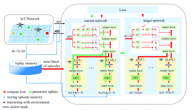
Figure 2: The framework of the QMIX algorithm in the training phase. The forward propagation process is represented by a solid red arrow, which is used to calculate the loss, while the backpropagation process is represented by a solid green arrow, which is used to update the parameters of the neural network. The top white box represents the mixing network and the bottom yellow boxes represent the agent networks. The blue arrow indicates the collection of the experience, and the black arrow indicates the interaction with environment. The black grid represents the action mask.

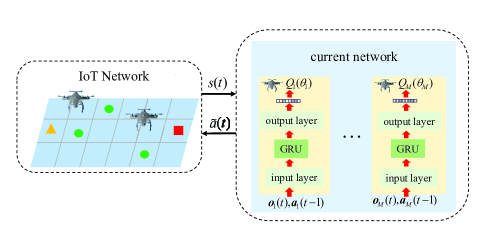
Figure 3: The framework of the QMIX algorithm in the testing phase.

IV-B1 Agent Network

For each UAV, there is an agent network to evaluates its local action-value function $Q_{m}(\boldsymbol{\tau}_{m}(t),\boldsymbol{a}_{m}(t);\theta_{m})$, where $\theta_{m}$ is the weights of the agent network. Each agent network has an input layer, a Gated Recurrent Unit (GRU) layer, and an output layer. The input layer of the agent network collects the current observation $\boldsymbol{o}_{m}(t)$ and the previous action $\boldsymbol{a}_{m}(t-1)$ of UAV $m$ and then feeds the joint observation-action history $\boldsymbol{\tau}_{m}(t)=(\boldsymbol{o}_{m}(t),\boldsymbol{a}_{m}(t-1))$ to the GRU layer. As an improved version of standard recurrent neural network, the GRU layer includes update gates and reset gates, which help capture long-term and short-term dependencies in sequences, respectively [39]. Hence, the GRU layer is able to overcome the partial observability of the underlying Dec-POMDP. Then, the GRU layer outputs its hidden states, which are fed to the output layer. Based on the hidden states of the GRU layer, the output layer produces the local action-value function.

Remark 1.

The computational complexity of training an agent network depends on the number of neurons in the input layer $h_{\text{I}}^{\text{a}}$, the GRU layer $h_{\text{G}}^{\text{a}}$, and the output layer $h_{\text{O}}^{\text{a}}$. Similar to [40], we can obtain the computational complexity of the GRU layer as $\mathcal{O}(h_{\text{G}}^{\text{a}}(3h_{\text{I}}^{\text{a}}+3h_{\text{G}}^{\text{a}}+h_{\text{O}}^{\text{a}}))$. Moreover, the computational complexity of a fully-connected layer with $h_{\text{I}}$ input and $h_{\text{O}}$ output neurons is $\mathcal{O}(h_{\text{I}}h_{\text{O}})$ [41]. Altogether, the computational complexity of training an agent network is $\mathcal{O}(h_{\text{I}}^{\text{a}}h_{\text{G}}^{\text{a}}+h_{\text{G}}^{\text{a}}(3h_{\text{I}}^{\text{a}}+3h_{\text{G}}^{\text{a}}+h_{\text{O}}^{\text{a}})+h_{\text{G}}^{\text{a}}h_{\text{O}}^{\text{a}})$, where $h_{\text{I}}^{\text{a}}$ and $h_{\text{O}}^{\text{a}}$ represent the dimensions of observation space and action space, respectively.

IV-B2 Mixing Network

The mixing network consists of a fully-connected neural network (FNN) with one hidden layer and a set of hypernetworks. The weights of the mixing network are denoted by $\theta_{0}$. We use the mixing network to evaluate the global action-value function $Q^{G}(\tilde{\boldsymbol{\tau}}(t),\tilde{\boldsymbol{a}}(t),$ $\boldsymbol{s}(t);\theta)$, where $\tilde{\bm{\tau}}(t)=(\bm{\tau}_{1}(t),\ldots,\bm{\tau}_{M}(t))$ and $\theta=(\theta_{0},\theta_{1},\ldots,\theta_{M})$. The input of the mixing network includes the output of each agent network, i.e., $Q_{m}(\boldsymbol{\tau}_{m},\boldsymbol{a}_{m}),\forall m\in\mathcal{M}$, and the state of the environment. In particular, the FNN takes the output of each agent network as its input and mixes them monotonically via a hidden layer. The output layer has only one neuron and produces the global action-value function. Different from a conventional FNN, the weights and biases of the FNN in the mixing network are produced by a set of hypernetworks. All the hypernetworks take the state $\boldsymbol{s}(t)$ as input so that $Q^{G}(\tilde{\boldsymbol{\tau}}(t),\tilde{\boldsymbol{a}}(t),\boldsymbol{s}(t);\theta)$ can be adjusted with respect to the state in a non-monotonic way. There are two hypernetworks that generate the weights between the input layer and the hidden layer, and those between the hidden layer and the output layer. Each of these two hypernetworks consists of one fully-connected (FC) layer. An absolute activation function is employed at the output of the FC layer to obtain the non-negative weights of the FNN. Moreover, the biases of the hidden layer and the output layer of the FNN are produced by another hypernetworks in a similar manner. In particular, we employ a hypernetwork with one FC layer to obtain the biases of the hidden layer, and a hypernetwork containing two FC layers with a rectified linear unit (ReLU) nonlinearity to obtain the biases of the output layer, respectively. With this structure, the mixing network guarantees that the global action-value function monotonically increases with a local action-value function [38], i.e.,

$$\frac{\partial Q^{G}(\tilde{\boldsymbol{\tau}}(t),\tilde{\boldsymbol{a}}(t),\boldsymbol{s}(t);\theta)}{\partial Q_{m}(\boldsymbol{\tau}_{m}(t),\boldsymbol{a}_{m}(t);\theta_{m})}\geq 0,\forall m\in\mathcal{M}.$$ (19)

As a result, the joint action that minimizes the global action-value function is equivalent to the individual actions that minimize each local action-value function. Specifically,

$$\arg\min_{\tilde{\boldsymbol{a}}}Q^{G}(\tilde{\boldsymbol{\tau}},\tilde{\boldsymbol{a}},\boldsymbol{s};\theta)=\left(\begin{array}[]{c}\arg\underset{\boldsymbol{a}_{1}}{\min}Q_{1}(\boldsymbol{\tau}_{1},\boldsymbol{a}_{1};\theta_{1})\\ \arg\underset{\boldsymbol{a}_{2}}{\min}Q_{2}(\boldsymbol{\tau}_{2},\boldsymbol{a}_{2};\theta_{2})\\ \vdots\\ \arg\underset{\boldsymbol{a}_{M}}{\min}Q_{M}(\boldsymbol{\tau}_{M},\boldsymbol{a}_{M};\theta_{M})\end{array}\right).$$ (20)

This allows each agent to greedily choose the action that minimizes its local action-value function in a decentralized way.

Remark 2.

The computational complexity of training the mixing network is dependent on the number of neurons in the FNN and those in the hypernetworks. Particularly, the computational complexity of the FNN with one hidden layer is $\mathcal{O}(h_{\text{I}}^{\text{m}}h_{\text{H}}^{\text{m}}+h_{\text{H}}^{\text{m}}h_{\text{O}}^{\text{m}})$, where $h_{\text{I}}^{\text{m}}$ is the number of neurons in the input layer, $h_{\text{H}}^{\text{m}}$ is the number of neurons in the hidden layer, and $h_{\text{O}}^{\text{m}}$ is the number of neurons in the output layer. Let $h_{\text{HI}}^{\text{m}}$ denote the number of neurons of the input layer of the hypernetworks. The computational complexity for two hypernetworks that generate the weights and biases between the input layer and the hidden layer are $\mathcal{O}(h_{\text{HI}}^{\text{m}}Mh_{\text{H}}^{\text{m}})$ and $\mathcal{O}(h_{\text{HI}}^{\text{m}}h_{\text{H}}^{\text{m}})$, respectively. Similarly, the computational complexity for two hypernetworks that generate the weights and bias between the hidden layer and the output layer are $\mathcal{O}(h_{\text{HI}}^{\text{m}}h_{\text{H}}^{\text{m}}h_{\text{O}}^{\text{m}})$ and $\mathcal{O}(h_{\text{HI}}^{\text{m}}h_{\text{H}}^{\text{m}}+h_{\text{H}}^{\text{m}}h_{\text{O}}^{\text{m}})$, respectively. Altogether, the computational complexity of the mixing network is

$$\mathcal{O}^{\textrm{m}}= \mathcal{O}(h_{\text{I}}^{\text{m}}h_{\text{H}}^{\text{m}}+h_{\text{H}}^{\text{m}}h_{\text{O}}^{\text{m}}+h_{\text{HI}}^{\text{m}}Mh_{\text{H}}^{\text{m}}+h_{\text{HI}}^{\text{m}}h_{\text{H}}^{\text{m}}+h_{\text{HI}}^{\text{m}}h_{\text{H}}^{\text{m}}h_{\text{O}}^{\text{m}}+h_{\text{HI}}^{\text{m}}h_{\text{H}}^{\text{m}}+h_{\text{H}}^{\text{m}}h_{\text{O}}^{\text{m}})$$

$$= \mathcal{O}(h_{\text{H}}^{\text{m}}(h_{\text{I}}^{\text{m}}+2h_{\text{O}}^{\text{m}}+(M+2+h_{\text{O}}^{\text{m}})h_{\text{HI}}^{\text{m}})).$$ (21)

Note that $h_{\text{HI}}^{\textrm{m}}$, $h_{\text{I}}^{\text{m}}$, and $h_{\text{O}}^{\text{m}}$ represent the dimensions of the state space, the number of agents $M$, and $1$, respectively.

IV-B3 Centralized Training

The centralized training of the agent networks and the mixing network is conducted offline. Similar to DQN, two sets of neural networks are used to stabilize the training process, as shown in Fig. 2. One is the current network with weights $\theta$ and the other is the target network with weights $\theta^{-}$. Here, the weights $\theta=(\theta_{0},\theta_{1},\ldots,\theta_{M})$ include the parameters of the mixing network $\theta_{0}$ and the parameters of all agent networks $\theta_{m}$ for $m\in\mathcal{M}$. The current network is used as a function approximator and its weights are updated at every slot. The target network calculates the target action-value function, and its weights are fixed for a period of time before being replaced with the latest weights from the current network at every O steps. Moreover, experience replay is also utilized. In order to efficiently train the GRU layer in each agent network, we sample the entire experience in an episode, rather than sampling transition tuples randomly in the reply memory as in DQN. This allows the hidden states of the GRU layer to learn the temporal correlations from the experience in the episode [42].

Algorithm 1 Training process of the multi-UAV enabled data collection algorithm.

1:  Initialize the current network $Q^{G}(\tilde{\boldsymbol{\tau}},\tilde{\boldsymbol{a}},\boldsymbol{s};\theta)$ and the target network $Q^{G}(\tilde{\boldsymbol{\tau}},\tilde{\boldsymbol{a}},\boldsymbol{s};\theta^{-})$;

2:  Initialize the replay memory $D$;

3:  for  $episode=1:EP$  do

4:     The environment initializes the initial state $\boldsymbol{s}(1)$ and the agent initializes its observation $\bm{o}_{m}(1)$;

5:     while  $\boldsymbol{s}(t)$ is not a terminal state do

6:        for  $\textrm{agent}\textrm{ }m=1:M$  do

7:           Compute available actions $\mathcal{A}_{m}^{\prime}(t)\triangleq\left(\mathcal{V}_{m}^{\prime}(t),\mathcal{B}_{m}^{\prime}(t)\right)$;

8:           Select a random action $\boldsymbol{a}_{m}(t)\in\mathcal{A}_{m}^{\prime}(t)$ with probability $\epsilon$;

9:           Otherwise select $\boldsymbol{a}_{m}(t)=\arg\min\limits_{\boldsymbol{a}_{m}\in\mathcal{A}_{m}^{\prime}(t)}Q_{m}(\bm{\tau}_{m}(t),\boldsymbol{a}_{m};\theta_{m}(t))$;

10:        end for

11:        Execute the joint action $\tilde{\boldsymbol{a}}(t)$, and get cost $c(t)$, next state $\boldsymbol{s}(t+1)$, and next joint observation $\tilde{\boldsymbol{o}}(t+1)$;

12:        Store the $(\boldsymbol{s}(t),\tilde{\boldsymbol{\tau}}(t),\tilde{\mathcal{A}}^{\prime}(t),\tilde{\boldsymbol{a}}(t),c(t),\boldsymbol{s}(t+1),\tilde{\boldsymbol{\tau}}(t+1),\tilde{\mathcal{A}}^{\prime}(t+1))$ in the replay memory;

13:        $\boldsymbol{s}(t)=\boldsymbol{s}(t+1)$ ;

14:     end while

15:     Sample a random mini-batch of episodes from $D$;

16:     Calculate the target action-value of the episode experiences $y^{G}$:

17:     for  $i=1:Z$ do

18:        if  $\boldsymbol{s}(i)$ is not the terminal state  then

19:           $y^{G}(i)=c(i)+\underset{\tilde{\boldsymbol{a}}\in\tilde{\mathcal{A}}^{\prime}(i+1)}{\min}Q^{G}(\tilde{\boldsymbol{\tau}}(i+1),\tilde{\boldsymbol{a}},\boldsymbol{s}(i+1);\theta^{-});$

20:        else

21:           $y^{G}(i)=c(i)$;

22:        end if

23:     end for

24:     $y^{G}=\mathop{\sum_{i=1}^{Z}y^{G}(i)}$;

25:     Update the current network by performing the gradient descent in (23);

26:     if  There are $O$ update-interval steps then

27:        Synchronize the target network by setting $\theta^{-}=\theta$;

28:     end if

29:  end for

The current network of QMIX is trained by minimizing the loss function at each episode. Specifically, the loss function with respect to the experiences in the episodes sampled from the replay memory is given by

$$L(\theta)=\mathop{\frac{1}{Z}\sum_{\textrm{$i=1$}}^{Z}}(y^{G}(i)-Q^{G}(\tilde{\boldsymbol{\tau}}(i),\tilde{\boldsymbol{a}}(i),\boldsymbol{s}(i);\theta))^{2},$$ (22)

where $Z$ is the number of transitions in the mini-batch and $y^{G}(i)=c(i)+\underset{\tilde{\boldsymbol{a}}\in\tilde{\mathcal{A}}^{\prime}(i+1)}{\min}Q^{G}(\tilde{\boldsymbol{\tau}}\left(i+1\right),$ $\tilde{\boldsymbol{a}},\boldsymbol{s}(i+1);\theta^{-})$. Here, $\tilde{\mathcal{A}}^{\prime}(i+1)=(\mathcal{A}^{\prime}_{1}(i+1),\ldots,\mathcal{A}^{\prime}_{M}(i+1))$ is the joint available actions of all UAVs in time slot $i+1$, and $\mathcal{A}^{\prime}_{m}(i+1)$ is the available actions of UAV $m$ in time slot $i+1$ obtained by the action mask method based on the observation $\boldsymbol{o}_{m}(i+1)$. Note that $Q^{G}(\tilde{\boldsymbol{\tau}}(i),\tilde{\boldsymbol{a}}(i),\boldsymbol{s}(i);\theta)$ and $Q^{G}(\tilde{\boldsymbol{\tau}}(i+1),\tilde{\boldsymbol{a}},\boldsymbol{s}(i+1);\theta^{-})$ are obtained by the current network and the target network, respectively. Afterward, the weights of the current network are updated by the semi-gradient algorithm as follows:

$$\theta=\theta+\frac{\alpha}{Z}\sum_{\textrm{$i=1$}}^{Z}(y^{G}(i)-Q^{G}(\tilde{\boldsymbol{\tau}}(i),\tilde{\boldsymbol{a}}(i),\boldsymbol{s}(i);\theta))\nabla_{\theta}Q^{G}(\tilde{\boldsymbol{\tau}}(i),\tilde{\boldsymbol{a}}(i),\boldsymbol{s}(i);\theta).$$ (23)

The details of the centralized training are summarized in Algorithm 1. First, the current network and target network are initialized and the replay memory is cleared out. Since the current network is updated based on the episodes of experiences, we gather the experience from an entire episode (Lines 5~14) before executing a gradient descent step (Line 25). Since the action mask filters out invalid actions which violate constraints (8c)-(8h), there are two cases making an episode terminate: 1) when two UAVs collide, $d_{m,m^{\prime}}(t)<d_{\textrm{safe}},m\neq m^{\prime},m,m^{\prime}\in\mathcal{M}$; 2) all the UAVs reach their final positions at time slot $T$. Before the terminal state, each agent chooses an action by utilizing the $\varepsilon$-greedy policy simultaneously, where $\varepsilon$ is decreasing with the increasing number of time slots $t$ (Lines 6~10). After all the agents conduct their actions, a cost $c(t)$ and the next observation $\tilde{\boldsymbol{o}}(t+1)$ can be obtained. The environment also transits to the next state $\boldsymbol{s}(t+1)$ (Line 11). Then, we randomly sample a mini-batch of episodes from the replay memory $D$ to update the current network (Lines 15~25). In every fixed $O$ episodes, the target network is updated by copying the current network parameters (Lines 26~28). Note that the number and position of SNs remain constant throughout all episodes.

IV-B4 Distributed Execution

When the offline centralized training is finished, the agent networks can be executed online in a decentralized manner. Particularly, each UAV make decisions in a distributed way by leveraging the pre-trained agent network based on its own observations. The testing framework of QMIX is shown in Fig. 3. Specifically, in every slot, each UAV chooses the action that minimizes its local action-value function, i.e., $\bm{a}_{m}(t)=\arg\min\limits_{\boldsymbol{a}_{m}\in\mathcal{A}_{m}^{\prime}(t)}Q_{m}(\boldsymbol{\tau}_{m},\boldsymbol{a}_{m};\theta_{m})$, and updates its observations accordingly. Each UAV continues its flight until it reaches its final position at the $T$-th slot. The details of the distributed execution are summarized in Algorithm 2.

Algorithm 2 Testing process of the multi-UAV enabled data collection algorithm.

1:  Initialize the environment;

2:  for  $episode=1:EPT$  do

3:     The environment initializes the initial state $\boldsymbol{s}(1)$ and the agent initializes its observation $\bm{o}_{m}(1)$;

4:     while  $\boldsymbol{s}(t)$ is not the terminal state do

5:        for  $\textrm{agent}\textrm{ }m=1:M$  do

6:            Compute available actions $\mathcal{A}_{m}^{\prime}(t)$;

7:           Select $\boldsymbol{a}_{m}(t)=\arg\min\limits_{\boldsymbol{a}_{m}\in\mathcal{A}_{m}^{\prime}(t)}Q_{m}(\bm{\tau}_{m}(t),\boldsymbol{a}_{m};\theta_{m}(t))$;

8:        end for

9:        Execute the joint action $\tilde{\boldsymbol{a}}(t)$, and get cost $c(t)$, next state $\boldsymbol{s}(t+1)$, and next joint observation $\tilde{\boldsymbol{o}}(t+1)$;

10:        $\boldsymbol{s}(t)=\boldsymbol{s}(t+1)$;

11:     end while

12:  end for

V Simulation Results

In this section, we conduct extensive simulations to evaluate the performance of our proposed algorithm. First, we describe the simulation setup and three baseline algorithms. Then, we evaluate the convergence and effectiveness of the proposed algorithm with respect to different system parameters.

V-A Simulation Setup

In the simulation, we deploy the SNs uniformly at random in a square area of $800\,\textrm{m}\times 800\,\textrm{m}$. Without loss of generality, we set the initial and final positions of the UAVs evenly at the bottom and top of the area, respectively. For example, if $M=3$, the UAVs’ initial locations will be $(0\,\textrm{m},0\,\textrm{m},100\,\textrm{m})$, $(360\,\textrm{m},0\,\textrm{m},100\,\textrm{m})$, and $(760\,\textrm{m},0\,\textrm{m},100\,\textrm{m})$, and the final locations will be $(0\,\textrm{m},760\,\textrm{m},100\,\textrm{m})$, $(360\,\textrm{m},760\,\textrm{m},100\,\textrm{m})$, and $(760\,\textrm{m},760\,\textrm{m},100\,\textrm{m})$. It is worth noting that the initial and final positions of each UAV can be the same, and the initial/final positions of different UAVs can also be the same. All the UAVs and the SNs are fully charged at the beginning of each episode. Unless otherwise stated, the simulation parameters of the IoT network can be found in Table I.

TABLE I: System parameters

Parameter	Value	Parameter	Value
Flight altitude $z$	$100\,$m [15]	Air density $\rho$	$1.225\,$kg/$\textrm{m}^{3}$
Time duration $T$	100 slots	Disc area for each rotor $A$	$0.0314\,\textrm{m}^{2}$
Slot length $\tau_{0}$	$0.5\,$s	Transmit power of each SN $P_{c}$	$5\,$mW [43]
Safe distance $d_{\textrm{safe}}$	$10\,$m	Noise power $\sigma^{2}$	$-110\,$dBm [44]
UAV maximum speed $v_{\max}^{s}$	$20\,$m/s [7]	$\beta_{0}$, $\beta_{1}$	11.95, 0.14 [45]
UAV maximum turning angle $\triangle\varphi_{\max}$	$\pi/3$	$\eta_{LoS}$, $\eta_{NLoS}$	$1.6\,$dB, $23\,$dB
Battery capacity $E_{\text{max}}$,$E_{\textrm{max}}^{\textrm{sn}}$	$2.4\times 10^{4}\,$J, $5\,$mJ	Carrier frequency$f_{c}$	$2\,$GHz [45]
$E_{\textrm{n}}^{\textrm{har}}$, $\lambda_{\textrm{n}}$	$0.42\,$mJ, $0.9$	Light speed in a vacuum $c$	$3\times 10^{8}\,$m/s
UAV mass $W$	$2\,$kg [7]	Number of rotors $n_{r}$	4
Gravity acceleration $g$	$9.8\,$m/$\textrm{s}^{2}$	$c_{f},c_{T}$	0.131, 0.302
Local blade section drag coefficient $\sigma$	0.012	$c_{s},d_{0}$	0.0955, 0.834

The QMIX-based algorithm is implemented by the PyTorch Library. Specifically, the agent network includes one GRU layer with $256$ hidden neurons. Since each UAV has the same state space and action space, the agent network of each UAV is identical [46]. The hidden layer in the mixing network contains $256$ neurons. The hyperparameters of the QMIX-based algorithm are listed in Table II.

TABLE II: Hyperparameters of the QMIX-based algorithm

Parameter	Value	Parameter	Value
The number of training episodes $EP$	50000	Minimum $\varepsilon$	0.01
$D,O$	1000, 200	Learning rate $\alpha$	0.0005
Mini-batch size	32	Optimizer	Adam
Initial $\varepsilon$	0.99	Activation function	ReLU
$\varepsilon$-greedy decrement	9.9e-6	$N_{1},N_{2}$	1, 6

In the following, we compare the proposed QMIX-based algorithm with three baseline algorithms:

• Nearest scheduling algorithm: This is a simplified version of the QMIX-based algorithm, where the trajectory is designed with the same method as in the multi-agent DRL approach, but each UAV schedules the SN with the nearest distance to itself.

• Cluster-based algorithm: In this algorithm, all the SNs are first clustered into $M$ clusters by K-means, with the initial positions of the cluster center being the start positions of the UAVs. Then, each UAV collects data from the SNs in its corresponding cluster. In each time slot, the UAV flies towards the SN with the largest AoI in its cluster and schedules the SN with the largest AoI within its coverage.

• IDQN-based algorithm: In this algorithm, each UAV works as an independent agent and employs DQN to address the trajectory design and the SN scheduling.

V-B Performance Evaluation

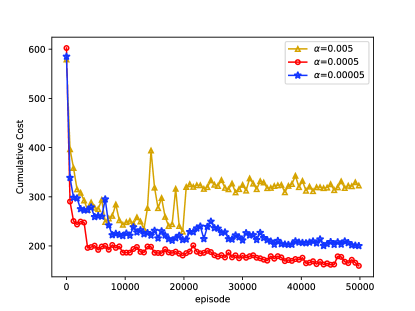
(a)

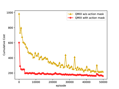
(b)

Figure 4: The convergence evaluation of our proposed QMIX-based algorithm ($\xi_{\textrm{th}}=5\textrm{ dB}$, $M=2$, and $N=15$). (a) The influence of different learning rates $\alpha$. (b) The influence of the action mask method.

We illustrate the convergence of the proposed QMIX-based algorithm in Fig. 4(a). In particular, the cumulative cost is plotted against the number of training episodes for different learning rates $\alpha$. As seen in the figure, a learning rate that is too high causes instability, while a rate that is too low leads to convergence at a local optimum. In this case, we find that the learning rate of 0.0005 performs best, as it produces the lowest cumulative cost compared to rates of 0.005 and 0.00005. This rate is therefore chosen for use with the QMIX algorithm in the following analysis. In Fig. 4(b), we examine the effect of the action mask method on QMIX’s convergence. By comparing QMIX with and without this method, we can see that the inclusion of the action mask leads to faster convergence and a lower cumulative cost. This is due to the mask’s ability to prevent invalid explorations by hiding actions that violate the constraints, thereby improving the performance of the QMIX algorithm.

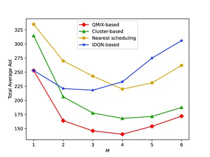
(a)

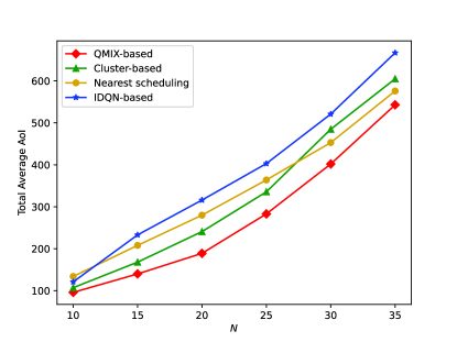
(b)

Figure 5: Comparison between QMIX-based algorithm and other three baseline algorithms ($\xi_{\textrm{th}}=5\textrm{ dB}$). (a) The total average AoI versus the number of UAVs $M$ with $N=15$. (b) The total average AoI versus the number of SNs $N$ with $M=4$.

Fig. 5(a) shows the total average AoI with respect to the number of UAVs $M$ with $N=15$ and $\xi_{\textrm{th}}=5\textrm{ dB}$. As $M$ increases, the total average AoI of the QMIX-based algorithm first decreases and then increases.This trend can be explained from two aspects. On the one hand, the average number of SNs that each UAV needs to schedule decreases as $M$ grows. Since each UAV can schedule no more than one SN at a time, each SN can be scheduled more frequently with more UAVs, resulting in a decrease in the total average AoI. On the other hand, the interference level also grows as $M$ increases. Hence, the probability of the status update being successfully received by the UAV is reduced, thereby raising the total average AoI. Clearly, the performance of the QMIX-based algorithm coincides with that of the IDQN-based algorithm when $M=1$, since they both degrade to single-agent DRL. Fig. 5(b) illustrates the total average AoI versus the number of SNs $N$ with $\xi_{\textrm{th}}=5\textrm{ dB}$ and $M=4$. We can see that the total average AoI increases as $N$ increases. This is because that each UAV can only schedule at most one SN to update its status at a time. Hence, the larger the number of SNs, the longer each SN must wait. Moreover, the total average AoI increases quickly as the number of SNs continues to increase. This is because, for a large $N$, more SNs have to wait to be scheduled by a limited number of UAVs, resulting in a rapid increase in the total average AoI. In both subfigures, the total average AoI of the proposed QMIX-based algorithm is lower than that of the other three baseline algorithms. This advantage is achieved by jointly optimizing the trajectories of UAVs and the scheduling of SNs through cooperative training of the UAVs with the global value function.

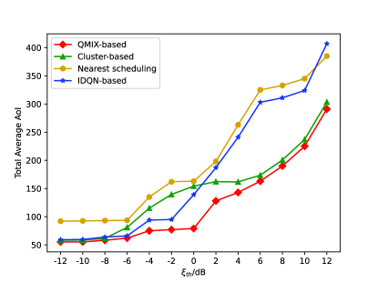
(a)

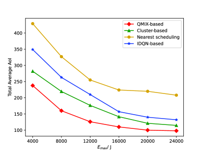
(b)

Figure 6: Comparison between QMIX-based algorithm and other three baseline algorithms ($N=15$). (a) The total average AoI versus the SINR threshold $\xi_{\textrm{th}}$ with $M=4$. (b) The total average AoI versus the total energy $E_{\textrm{max}}$ with $\xi_{\textrm{th}}=5\textrm{ dB and }M=3$.

Fig. 6(a) shows the total average AoI versus the threshold $\xi_{\textrm{th}}$ with $N=15$ and $M=4$. From Fig. 6(a), we can see that the total average AoI increases as $\xi_{\textrm{th}}$ increases. This is due to the fact that the probability of successful transmission decreases with a larger $\xi_{\textrm{th}}$ , resulting in a higher total average AoI. It can also be seen that, while the cluster-based algorithm performs similarly to the QMIX-based algorithm in both the low and high regimes of $\xi_{\textrm{th}}$, the QMIX-based algorithm consistently has the lowest total average AoI across all regimes of $\xi_{\textrm{th}}$. Fig. 6(b) evaluates the total average AoI versus the UAV’s battery capacity $E_{\textrm{max}}$ with $N=15$, $\xi_{\textrm{th}}=5\textrm{dB}$, and $M=3$. The initial and final locations are set to the same, with the UAVs starting at $(0\,\textrm{m},360\,\textrm{m},100\,\textrm{m})$, $(360\,\textrm{m},360\,\textrm{m},100\,\textrm{m})$, and $(760\,\textrm{m},360\,\textrm{m},100\,\textrm{m})$, respectively. The energy consumed by a UAV in one time slot is mainly determined by the UAV’s speed and acceleration, as shown in Eq. (1). From Fig. 6(b), we can see that the total average AoI decreases sharply with $E_{\textrm{max}}$ at first and then decreases more slowly. The reason is that the energy constraint is tight when $E_{\textrm{max}}$ is small, requiring the UAV to hover in some slots to conserve energy. When $E_{\textrm{max}}$ is larger, the energy constraint is less restrictive, allowing the UAV to move more freely to collect packets.

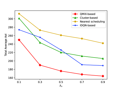
Figure 7: The total average AoI versus the SN’s energy arrival probability $\lambda_{n}$ with $N=15$, $\xi_{\textrm{th}}=5\textrm{dB}$, and $M=2$.

Fig. 7 shows the effect of SN’s energy arrival probability $\lambda_{n}$ on the total average AoI with $N=15$, $\xi_{\textrm{th}}=5\textrm{dB}$, and $M=2$. From Fig. 7, we can see that as $\lambda_{n}$ increases, the total average AoI decreases. This is because when $\lambda_{n}$ is small, the energy of the SN is insufficient, resulting in untimely status updates due to the lack of energy. However, as $\lambda_{n}$ increases, the SN is more likely to have enough energy to update when the UAV flies to its vicinity. When $\lambda_{n}\geq 0.7$, the decrease in total average AoI becomes marginal because the SN can be charged in time. We can also see that the QMIX-based algorithm achieves the lowest total average AoI compared to other baseline algorithms. This is because the QMIX-based algorithm can jointly optimize UAVs’ trajectories and scheduling strategies, even when $\lambda_{n}$ is small, and effectively adjust them to reduce the total average AoI.

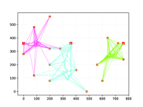
(a)

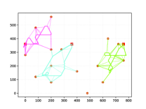
(b)

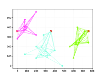
(c)

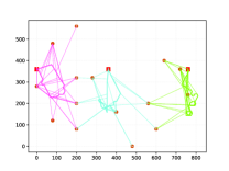
(d)

(e)

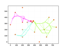
(f)

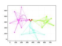
(g)

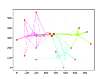
(h)

Figure 8: An illustration of the trajectories of UAVs and scheduling of SNs in one episode ($\xi_{\textrm{th}}=7\textrm{ dB}$, $N=15$, $p_{h}=0.9$, and $M=3$). (a) QMIX-based algorithm with initial and final positions far apart. (b) Nearest scheduling algorithm with initial and final positions far apart. (c) Cluster-based algorithm with initial and final positions far apart. (d) IDQN-based algorithm with initial and final positions far apart. (e) QMIX-based algorithm with close initial and final positions. (f) Nearest scheduling algorithm with close initial and final positions. (g) Cluster-based algorithm with close initial and final positions. (h) IDQN-based algorithm with close initial and final positions.

Fig. 8 displays the trajectories of UAVs and the scheduling of SNs in different algorithms. The solid line indicates the trajectory of the UAV, while the dashed line represents the scheduling of SNs. Moreover, we use different colors to denote different UAVs and their scheduled SNs. For each UAV, its initial and final locations are set to the same and represented by squares in the figures. In Figs. 8(a)-(d), the initial and final positions of the UAVs are far apart, while in Figs. 8(e)-(h), the initial and final positions are close to each other. In Fig. 8(a), the multiple UAVs can fly to and schedule the SNs cooperatively so as to reduce the interference and the total average AoI. However, in Fig. 8(b), the scheduling of the SNs are not coordinated in the nearest scheduling algorithm, resulting in higher interference. In Fig. 8(c), the trajectories of the UAVs are suboptimal in the cluster-based algorithm because the status updates of SNs can only be collected by a specific UAV once they are clustered. In Fig. 8(d), the IDQN-based algorithm can only optimize the trajectories of individual UAVs and the scheduling of SNs separately, resulting in a local optimal solution. As shown in Figs. 8(e)-(h), our approach can also work well in scenarios where the initial and final locations of the UAVs are close to each other. Through the comparison, we can see that the UAVs in the QMIX-based algorithms are able to divide the workload and collect data from different SNs. Additionally, they can cooperate to collect data for some SNs, resulting in a reduction of the total average AoI.

The comparisons of complexity and performance between our proposed algorithm and other baseline algorithms are summarized in Table III. The complexity of the Cluster-based algorithm is primarily determined by the K-means algorithm, which has a complexity of $\mathcal{O}(MN)$. On the other hand, the complexity of the QMIX-based, Nearest Scheduling, and IDQN-based algorithms is mainly determined by the computation of their neural networks. The QMIX-based algorithm and the Nearest Scheduling algorithm have the same agent and mixing networks, but the output layer of the agent network in the Nearest Scheduling algorithm is smaller. To clearly illustrate the difference, the computational complexity of the agent network $\mathcal{O}^{\textrm{a}}$ is denoted as a function of the output dimension of the agent network $h_{\text{O}}$. The IDQN-based algorithm has the same agent networks as the QMIX-based algorithm, but lacks the mixing network. Therefore, the complexity of the QMIX-based algorithm is higher than that of other baseline algorithms. The table also shows the total average AoI for all baseline algorithms and our proposed algorithm, which was obtained with $N=15,M=4,E_{\max}=2.4\times 10^{4}\,\textrm{J},\textrm{ and }\xi_{\textrm{th}}=5\,\textrm{dB}$. We can see that the QMIX-based algorithm achieves the best performance.

TABLE III: Computational complexity and performance comparisons

Method	Computational Complexity	Total average AoI
QMIX-based	$M\mathcal{O}^{\textrm{a}}((N+1)(N_{1}+1)(N_{2}+1))+\mathcal{O}^{\textrm{m}}$	140
Cluster-based	$\mathcal{O}(MN)$	168.1
Nearest scheduling	$M\mathcal{O}^{\textrm{a}}((N_{1}+1)(N_{2}+1))+\mathcal{O}^{\textrm{m}}$	208
IDQN-based	$M\mathcal{O}^{\textrm{a}}((N+1)(N_{1}+1)(N_{2}+1))$	233

VI Conclusions

In this study, we examined the problem of optimally collecting data in multi-UAV enabled IoT networks using multiple cooperative UAVs. We took into account kinematic, energy, trajectory, and collision avoidance constraints and aimed to minimize the total average AoI. To accomplish this goal, we proposed the QMIX-based algorithm to jointly optimize the trajectories of the UAVs and the scheduling of the SNs. Particularly, the UAVs were centrally trained using a global value function, and then each UAV carried out data collection in a distributed manner based on its local observations. Our simulation results showed that the proposed QMIX-based algorithm was superior to other baseline approaches and the action mask method helped accelerate the convergence of the QMIX-based algorithm. We observed that the UAVs in the QMIX-based algorithm were able to divide their workload and collect data from different SNs, and in some cases even cooperated in collecting data from the same SN. We also found that there is an optimal number of UAVs that minimizes the total average AoI due to the tradeoff between increased transmission opportunities and higher mutual interference. In the future work, we will consider optimizing of trajectory planning transmission scheduling based on the NR frame structure, where the UAV trajectory can be optimized on a large timescale, and the transmission scheduling is optimized on a small time scale.

Appendix A Proof for The Property of $\phi_{m}(t+1)\geq\phi_{m}(t)-4$ and $\psi_{m}(t+1)\geq\psi_{m}(t)-4\overline{E}$

When the UAV is able to immediately turn its velocity direction towards the destination at the beginning of slot $t$, i.e., $\triangle\varphi_{m}^{\textrm{stop}}(t)\leq\triangle\varphi_{\max}\textrm{ or }v_{m}^{s}(t)=0$, and the direction of velocity at the beginning of slot $t+1$ is opposite to the direction of the current position pointing towards the destination, i.e., $\varphi_{m}(t+1)=\varphi_{m}^{\textrm{stop}}(t)+\pi$, the minimum values of $(\phi_{m}(t+1)-\phi_{m}(t))$ and $(\psi_{m}(t+1)-\psi_{m}(t))$ are obtained.

In this case, $\bm{u}_{m}(t+1)$, $\bm{u}_{m}(t)$, and $\bm{u}_{m}^{\text{stop}}$ are on a straight line. Hence, we have $\left\|\bm{u}_{m}(t)-\bm{u}_{m}^{\text{stop}}\right\|-\left\|\bm{u}_{m}(t+1)-\bm{u}_{m}^{\text{stop}}\right\|=-\frac{v_{m}^{s}(t)+v_{m}^{s}(t+1)}{2}\tau_{0}$. Then, we can obtain

$$T_{m}^{\textrm{req}}(t)-T_{m}^{\textrm{req}}(t+1)$$

$$= \left\lceil\frac{\left\|\bm{u}_{m}(t)-\bm{u}_{m}^{\text{stop}}\right\|-\frac{v_{m}^{s}(t)+v_{\max}^{s}}{2}\tau_{0}}{v_{\max}^{s}\tau_{0}}\right\rceil-\left\lceil\frac{\left\|\bm{u}_{m}(t+1)-\bm{u}_{m}^{\text{stop}}\right\|+\frac{v_{m}^{s}(t+1)-v_{\max}^{s}}{2}\tau_{0}}{v_{\max}^{s}\tau_{0}}\right\rceil-1$$

$$\overset{(a)}{\geq} \left\lfloor\frac{-\frac{v_{m}^{s}(t)+v_{m}^{s}(t+1)}{2}-\frac{v_{m}^{s}(t)+v_{\max}^{s}}{2}-\frac{v_{m}^{s}(t+1)-v_{\max}^{s}}{2}}{v_{\max}^{s}}\right\rfloor-1$$

$$= \left\lfloor\frac{-v_{m}^{s}(t)-v_{m}^{s}(t+1)}{v_{\max}^{s}}\right\rfloor-1$$

$$\geq -3,$$ (24)

where (a) is due to the fact that $\lceil i\rceil-\lceil j\rceil\geq\lfloor i-j\rfloor$. Bringing (24) into (13), we can get that $\phi_{m}(t+1)\geq\phi_{m}(t)-4.$

By assuming the maximum energy consumption $\overline{E}$ in each time slot, we can obtain that $\psi_{m}(t)-\psi_{m}(t+1)\leq 4\overline{E}$ due to $\phi_{m}(t)-\phi_{m}(t+1)\leq 4$. Hence, we have $\psi_{m}(t+1)\geq\psi_{m}(t)-4\overline{E}$.

References

- [1] M. Yi, X. Wang, J. Liu, Y. Zhang, and B. Bai, “Deep Reinforcement Learning for Fresh Data Collection in UAV-assisted IoT Networks,” in Proc. IEEE INFOCOM WKSHPS, July 2020.
- [2] M. Mozaffari, W. Saad, M. Bennis, Y. Nam, and M. Debbah, “A Tutorial on UAVs for Wireless Networks: Applications, Challenges, and Open Problems,” IEEE Commun. Surv. Tutorials, vol. 21, no. 3, pp. 2334–2360, 2019.
- [3] Y. Zeng, Q. Wu, and R. Zhang, “Accessing From the Sky: A Tutorial on UAV Communications for 5G and Beyond,” Proc. IEEE, vol. 107, no. 12, pp. 2327–2375, Dec 2019.
- [4] J. Gong, T. Chang, C. Shen, and X. Chen, “Flight Time Minimization of UAV for Data Collection Over Wireless Sensor Networks,” IEEE J. Sel. Areas Commun., vol. 36, no. 9, pp. 1942–1954, 2018.
- [5] Y. Zeng and R. Zhang, “Energy-Efficient UAV Communication With Trajectory Optimization,” IEEE Trans. Wireless Commun., vol. 16, no. 6, pp. 3747–3760, 2017.
- [6] C. H. Liu, Z. Chen, J. Tang, J. Xu, and C. Piao, “Energy-Efficient UAV Control for Effective and Fair Communication Coverage: A Deep Reinforcement Learning Approach,” IEEE J. Sel. Areas Commun., vol. 36, no. 9, pp. 2059–2070, 2018.
- [7] R. Ding, F. Gao, and X. S. Shen, “3D UAV Trajectory Design and Frequency Band Allocation for Energy-Efficient and Fair Communication: A Deep Reinforcement Learning Approach,” IEEE Trans. Wireless Commun., vol. 19, no. 12, pp. 7796–7809, 2020.
- [8] M. Pourghasemian, M. R. Abedi, S. S. Hosseini, N. Mokari, M. R. Javan, and E. A. Jorswieck, “AI-Based Mobility-Aware Energy Efficient Resource Allocation and Trajectory Design for NFV Enabled Aerial Networks,” IEEE Trans. Green Commun. Netw., pp. 1–1, 2022.
- [9] M. A. Abd-Elmagid, N. Pappas, and H. S. Dhillon, “On the Role of Age of Information in the Internet of Things,” IEEE Commun. Mag., vol. 57, no. 12, pp. 72–77, 2019.
- [10] O. M. Bushnaq, A. Chaaban, and T. Y. Al-Naffouri, “The Role of UAV-IoT Networks in Future Wildfire Detection,” IEEE Internet Things J., vol. 8, no. 23, pp. 16 984–16 999, 2021.
- [11] S. Kaul, M. Gruteser, V. Rai, and J. Kenney, “Minimizing Age of Information in Vehicular Networks,” in Proc. IEEE 8th Annu. Commun. Soc. Conf. Sensor, Mesh, Ad Hoc Commun. Netw., 2011, pp. 350–358.
- [12] M. Akbari, M. R. Abedi, R. Joda, M. Pourghasemian, N. Mokari, and M. Erol-Kantarci, “Age of Information Aware VNF Scheduling in Industrial IoT Using Deep Reinforcement Learning,” IEEE J. Sel. Areas Commun., vol. 39, no. 8, pp. 2487–2500, 2021.
- [13] C. Guo, X. Wang, L. Liang, and G. Y. Li, “Age of information, latency, and reliability in intelligent vehicular networks,” IEEE Network, pp. 1–8, 2022.
- [14] J. Hu, H. Zhang, L. Song, R. Schober, and H. V. Poor, “Cooperative Internet of UAVs: Distributed Trajectory Design by Multi-Agent Deep Reinforcement Learning,” IEEE Trans. Commun., vol. 68, no. 11, pp. 6807–6821, 2020.
- [15] F. Wu, H. Zhang, J. Wu, Z. Han, H. V. Poor, and L. Song, “UAV-to-Device Underlay Communications: Age of Information Minimization by Multi-Agent Deep Reinforcement Learning,” IEEE Trans. Commun., vol. 69, no. 7, pp. 4461–4475, 2021.
- [16] W. Li, L. Wang, and A. Fei, “Minimizing Packet Expiration Loss With Path Planning in UAV-Assisted Data Sensing,” IEEE Wirel. Commun. Lett., vol. 8, no. 6, pp. 1520–1523, Dec. 2019.
- [17] J. Liu, P. Tong, X. Wang, B. Bai, and H. Dai, “UAV-Aided Data Collection for Information Freshness in Wireless Sensor Networks,” IEEE Trans. Wireless Commun., pp. 1–1, 2020.
- [18] H. Hu, K. Xiong, G. Qu, Q. Ni, P. Fan, and K. B. Letaief, “AoI-Minimal Trajectory Planning and Data Collection in UAV-Assisted Wireless Powered IoT Networks,” IEEE Internet Things J., vol. 8, no. 2, pp. 1211–1223, 2021.
- [19] Z. Jia, X. Qin, Z. Wang, and B. Liu, “Age-Based Path Planning and Data Acquisition in UAV-Assisted IoT Networks,” in Proc. IEEE Int. Conf. Commun. Workshops (ICC Workshops), 2019, pp. 1–6.
- [20] M. A. Abd-Elmagid, A. Ferdowsi, H. S. Dhillon, and W. Saad, “Deep Reinforcement Learning for Minimizing Age-of-Information in UAV-Assisted Networks,” in Proc. IEEE Global Commun. Conf. (GLOBECOM), Puako, HI, USA, May 2019.
- [21] A. Ferdowsi, M. A. Abd-Elmagid, W. Saad, and H. S. Dhillon, “Neural Combinatorial Deep Reinforcement Learning for Age-Optimal Joint Trajectory and Scheduling Design in UAV-Assisted Networks,” IEEE J. Sel. Areas Commun., vol. 39, no. 5, pp. 1250–1265, 2021.
- [22] M. A. Abd-Elmagid and H. S. Dhillon, “Average Peak Age-of-Information Minimization in UAV-assisted IoT Networks,” IEEE Trans. Veh. Technol., vol. 68, no. 2, pp. 2003–2008, 2019.
- [23] S. Zhang, H. Zhang, Z. Han, H. V. Poor, and L. Song, “Age of Information in a Cellular Internet of UAVs: Sensing and Communication Trade-Off Design,” IEEE Trans. Wireless Commun., vol. 19, no. 10, pp. 6578–6592, 2020.
- [24] M. Sun, X. Xu, X. Qin, and P. Zhang, “AoI-Energy-Aware UAV-Assisted Data Collection for IoT Networks: A Deep Reinforcement Learning Method,” IEEE Internet Things J., vol. 8, no. 24, pp. 17 275–17 289, 2021.
- [25] M. Samir, C. Assi, S. Sharafeddine, D. Ebrahimi, and A. Ghrayeb, “Age of Information Aware Trajectory Planning of UAVs in Intelligent Transportation Systems: A Deep Learning Approach,” IEEE Trans. Veh. Technol., vol. 69, no. 11, pp. 12 382–12 395, 2020.
- [26] S. F. Abedin, M. S. Munir, N. H. Tran, Z. Han, and C. S. Hong, “Data Freshness and Energy-Efficient UAV Navigation Optimization: A Deep Reinforcement Learning Approach,” IEEE Trans. Intell. Transp. Syst., pp. 1–13, 2020.
- [27] O. S. Oubbati, M. Atiquzzaman, A. Lakas, A. Baz, H. Alhakami, and W. Alhakami, “Multi-UAV-enabled AoI-aware WPCN: A Multi-agent Reinforcement Learning Strategy,” in Proc. IEEE Int. Conf. Comput. Commun. Workshops (INFOCOM WKSHPS), 2021, pp. 1–6.
- [28] A. Baknina and S. Ulukus, “Optimal and Near-Optimal Online Strategies for Energy Harvesting Broadcast Channels,” IEEE J. Sel. Areas Commun., vol. 34, no. 12, pp. 3696–3708, 2016.
- [29] D. Shaviv and A. Ozgur, “Universally Near Optimal Online Power Control for Energy Harvesting Nodes,” IEEE J. Sel. Areas Commun., vol. 34, no. 12, pp. 3620–3631, 2016.
- [30] A. Arafa, J. Yang, S. Ulukus, and H. V. Poor, “Age-Minimal Transmission for Energy Harvesting Sensors With Finite Batteries: Online Policies,” IEEE Trans. Inf. Theory, vol. 66, no. 1, pp. 534–556, 2020.
- [31] A. Al-Hourani, S. Kandeepan, and S. Lardner, “Optimal LAP Altitude for Maximum Coverage,” IEEE Wireless Commun. Lett., vol. 3, no. 6, pp. 569–572, 2014.
- [32] Y. Zeng, X. Xu, and R. Zhang, “Trajectory Design for Completion Time Minimization in UAV-Enabled Multicasting,” IEEE Trans. Wireless Commun., vol. 17, no. 4, pp. 2233–2246, 2018.
- [33] L. Liu, K. Xiong, J. Cao, Y. Lu, P. Fan, and K. B. Letaief, “Average AoI Minimization in UAV-Assisted Data Collection With RF Wireless Power Transfer: A Deep Reinforcement Learning Scheme,” IEEE Internet Things J., vol. 9, no. 7, pp. 5216–5228, 2022.
- [34] F. A. Oliehoek, C. Amato et al., A concise introduction to decentralized POMDPs. Springer, 2016, vol. 1.
- [35] C. J. Watkins and P. Dayan, “Q-learning,” Machine learning, vol. 8, no. 3, pp. 279–292, 1992.
- [36] R. S. Sutton and A. G. Barto, Reinforcement learning: An introduction. MIT press, 2018.
- [37] A. Tampuu, T. Matiisen, D. Kodelja, I. Kuzovkin, K. Korjus, J. Aru, J. Aru, and R. Vicente, “Multiagent Cooperation and Competition with Deep Reinforcement Learning,” PloS one, vol. 12, no. 4, p. e0172395, 2017.
- [38] T. Rashid, M. Samvelyan, C. S. De Witt, G. Farquhar, J. Foerster, and S. Whiteson, “QMIX: Monotonic Value Function Factorisation for Deep Multi-Agent Reinforcement Learning,” arXiv:1803.11485, 2018.
- [39] J. Chung, C. Gulcehre, K. Cho, and Y. Bengio, “Empirical Evaluation of Gated Recurrent Neural Networks on Sequence Modeling,” arXiv:1412.3555, 2014.
- [40] H. Sak, A. Senior, and F. Beaufays, “Long Short-Term Memory Based Recurrent Neural Network Architectures for Large Vocabulary Speech Recognition,” arXiv:1402.1128, p. arXiv:1402.1128, Feb. 2014.
- [41] J. Wu, C. Leng, Y. Wang, Q. Hu, and J. Cheng, “Quantized Convolutional Neural Networks for Mobile Devices,” in Proc. IEEE Conf. Comput. Vis. Pattern Recognit. (CVPR), June 2016.
- [42] M. Hausknecht and P. Stone, “Deep Recurrent Q-Learning for Partially Observable MDPs,” arXiv:1507.06527, 2015.
- [43] S. Leng and A. Yener, “Age of Information Minimization for Wireless Ad Hoc Networks: A Deep Reinforcement Learning Approach,” in Proc. IEEE Global Commun. Conf. (GLOBECOM). IEEE, 2019, pp. 1–6.
- [44] H. Hu, K. Xiong, G. Qu, Q. Ni, P. Fan, and K. B. Letaief, “AoI-Minimal Trajectory Planning and Data Collection in UAV-Assisted Wireless Powered IoT Networks,” IEEE Internet Things J., vol. 8, no. 2, pp. 1211–1223, 2021.
- [45] M. Mozaffari, W. Saad, M. Bennis, and M. Debbah, “Mobile Unmanned Aerial Vehicles (UAVs) for Energy-Efficient Internet of Things Communications,” IEEE Trans. Wireless Commun., vol. 16, no. 11, pp. 7574–7589, 2017.
- [46] J. Foerster, I. A. Assael, N. De Freitas, and S. Whiteson, “Learning to Communicate with Deep Multi-Agent Reinforcement Learning,” in Proc. 29th Adv. Neural Inf. Process. Syst. (NeurIPS), 2016, pp. 2137–2145.