Noda Iteration for Computing Generalized Tensor Eigenpairs

Abstract

In this paper, we propose the tensor Noda iteration (NI) and its inexact version for solving the eigenvalue problem of a particular class of tensor pairs called generalized $\mathcal{M}$-tensor pairs. A generalized $\mathcal{M}$-tensor pair consists of a weakly irreducible nonnegative tensor and a nonsingular $\mathcal{M}$-tensor within a linear combination. It is shown that any generalized $\mathcal{M}$-tensor pair admits a unique positive generalized eigenvalue with a positive eigenvector. A modified tensor Noda iteration(MTNI) is developed for extending the Noda iteration for nonnegative matrix eigenproblems. In addition, the inexact generalized tensor Noda iteration method (IGTNI) and the generalized Newton-Noda iteration method (GNNI) are also introduced for more efficient implementations and faster convergence. Under a mild assumption on the initial values, the convergence of these algorithms is guaranteed. The efficiency of these algorithms is illustrated by numerical experiments.

Key words.  generalized tensor eigenproblem, modified Noda iteration, generalized Noda iteration, inexact algorithm, Newton’s method, nonnegative tensor, $\mathcal{M}$–tensor, positive preserving

1 Introduction

Tensor spectral theory and eigenvalue problems with a vast range of applications are widely investigated [10, 21, 47, 48]. Variant versions of tensor eigenvalues are introduced from different aspects of generalizing from the matrix counterpart. Some recent papers [8, 17, 35] point out that this generalized eigenvalue framework unifies several definitions of tensor eigenvalues. Generalized tensor eigenvalue problems have been extensively studied due to their wide applications such as higher-order Markov chain [15], quantum information processing [43], and multilabel learning [50].

A tensor $\operatorname{\mathcal{A}}=(a_{i_{1}\ldots i_{m}})$ is a multi-array of entries $a_{i_{1}\ldots i_{m}}\in\mathbf{F}$, where $i_{j}=1,\ldots,n_{j}$ for $j=1,\ldots,m$ and $\mathbf{F}$ is a field. In this paper, we only consider real tensors, i.e., $\mathbf{F}=\mathbb{R}$. When $n=n_{1}=\cdots=n_{m}$, $\operatorname{\mathcal{A}}$ is called an $m$th order $n$-dimensional tensor. Denote the set of all $m$th order $n$-dimensional real tensors as $T_{m,n}$. For any tensor $\operatorname{\mathcal{A}}\in T_{m,n}$ and any vector $\mathbf{x}\in\mathbb{R}^{n}$, the tensor-vector multiplication $\operatorname{\mathcal{A}}\mathbf{x}^{m-1}$ is defined by

$$\operatorname{\mathcal{A}}\mathbf{x}^{m-1}=\left(\sum\limits_{i_{2},\ldots,i_{m}=1}^{n}a_{ii_{2}\cdots i_{m}}x_{i_{2}}\cdots x_{i_{m}}\right)\in\mathbb{R}^{n}.$$

The definition of tensor eigenvalues was proposed by Qi [46] and Lim [36] independently in 2005. Let $\operatorname{\mathcal{A}}=(a_{i_{1}\cdots i_{m}})\in T_{m,n}$. We call a number $\lambda\in\mathbb{C}$ an eigenvalue of $\operatorname{\mathcal{A}}$ if there exists a nonzero vector $\mathbf{x}\in\mathbb{C}^{n}$ satisfying the homogeneous polynomial equations:

$$\operatorname{\mathcal{A}}\mathbf{x}^{m-1}=\lambda\mathbf{x}^{[m-1]},$$ (1.1)

where the notation $\mathbf{x}^{[m-1]}$ for $\mathbf{x}=(x_{1},\ldots,x_{n})^{\top}\in\mathbb{C}^{n}$ is defined by $\mathbf{x}^{[m-1]}=(x_{1}^{m-1},\ldots,x_{n}^{m-1})^{\top}$. Then we call the nonzero vector $\mathbf{x}$ an eigenvector of $\operatorname{\mathcal{A}}$ associated with the eigenvalue $\lambda$ and the pair $(\mathbf{x},\lambda)$ an eigenpair of $\operatorname{\mathcal{A}}$. The set of all eigenvalues of a tensor is called its spectrum. The largest modulus of the elements in the spectrum of $\operatorname{\mathcal{A}}$ is denoted as $\rho(\operatorname{\mathcal{A}})$.

Chang, Pearson, and Zhang [8] first introduced the generalized eigenvalues, called the $\mathcal{B}$-eigenvalues for a tensor $\mathcal{A}$ in their paper. Let $\mathcal{A}$ and $\mathcal{B}$ be two square tensors of the same size. Supposing that $\lambda\in\mathbb{C}$ and $\mathbf{x}\in\mathbb{C}^{n}$ satisfy

$$\mathcal{A}\mathbf{x}^{m-1}=\lambda\mathcal{B}\mathbf{x}^{m-1},~{}\mathbf{x}\neq\mathbf{0},$$ (1.2)

we call $\lambda$ a $\mathcal{B}$–eigenvalue of $\mathcal{A}$ and $\mathbf{x}$ the associated $\mathcal{B}$–eigenvector. Ding and Wei [19] further investigated the perturbation and error analysis of the generalized eigenvalue problem systematically.

Some frequently used notations are introduced as follows. For any real tensor $\mathcal{A}=(a_{i_{1}\ldots i_{m}})\in T_{m,n}$, we say that $\mathcal{A}$ is nonnegative, and write $\mathcal{A}\geq 0$, if $a_{i_{1}\ldots i_{m}}\geq 0$ for all $i_{1},\ldots,i_{m}$. The tensor $\mathcal{A}$ is called positive, $\mathcal{A}>0$, if $a_{i_{1}\ldots i_{m}}>0$ for all $i_{1},\ldots,i_{m}$. If $\mathcal{A},\mathcal{B}\in T_{m,n}$, then $\mathcal{A}\geq\mathcal{B}$ $(\mathcal{A}>\mathcal{B})$ means that $a_{i_{1}\ldots i_{m}}\geq b_{i_{1}\ldots i_{m}}(a_{i_{1}\ldots i_{m}}>b_{i_{1}\ldots i_{m}})$ for all $i_{1},\ldots,i_{m}$. A nonnegative (positive) vector or matrix is defined in the same way.

For real vectors $\mathbf{x}=(x_{1},x_{2},\ldots,x_{n})^{\top}$ and $\mathbf{y}=(y_{1},y_{2},\ldots,y_{n})^{\top}$ with $y_{i}\neq 0$ for all $i$, we use $\frac{\mathbf{x}}{\mathbf{y}}$ to denote the column vector whose $i$-th component is $\frac{x_{i}}{y_{i}}$. We also define $\max\mathbf{x}=\max\limits_{i}x_{i}$ and $\min\mathbf{x}=\min\limits_{i}x_{i}$. We denote $\mathbf{x}^{[m-1]}=(x_{1}^{m-1},\ldots,x_{n}^{m-1})^{\top}$ and $[n]=\{1,2,\ldots,n\}$. For simplicity, we use $\|\cdot\|$ to denote the 2–norm for vectors and matrices in this paper.

Several numerical methods have been proposed in the literature for computing generalized eigenpairs for different classes of tensor pairs. Kolda and Mayo [35] proposed a power method for computing the generalized eigenpairs for symmetric tensor pair. In Cui, Dai, and Nie [17], a semidefinite relaxation method was developed to find all real eigenvalues of symmetric tensor pairs. In [11, 12], Chen, Han and Zhou presented the homotopy methods for computing the (generalized) tensor eigenpair. Yu, Yu, Xu, Song, and Zhou [54] gave an adaptive gradient method for computing generalized tensor eigenpairs. Zhao, Yang and Liu [56] computed the generalized eigenvalues of weakly symmetric tensors. Che, Cichocki and Wei [9] applied the neural dynamical network to compute a best rank-one approximation of a real- valued tensor and solve the tensor eigenvalue problems. Mo, Wang and Wei [40] explored time-varying generalized tensor eigenanalysis via Zhang neural networks.

In this paper, inspired by the work of Chen, Vong, Li, and Xu [13], we will prove an extension of the Perron-Frobenius theory for a special kind of tensor pair and present iteration methods for finding the Perron pair of this special kind of tensor pair. Chen, Vong, Li, and Xu [13] considered the generalized eigenvalue problem of a special type of matrix pairs that exhibits the same kind of properties of nonnegative matrices provided by the Perron-Frobenius theory. Motivated by the nonlinear extension of the Perron-Frobenius theory in [41], Fujimoto [24] considered the matrix generalized eigenproblem $A\mathbf{x}=\lambda B\mathbf{x}$ satisfying the following conditions:

1. $A\geq 0.$

2. $A$ is irreducible.

3. There exists a vector $\mathbf{v}>0$ such that $B\mathbf{v}>A\mathbf{v}$.

4. For all $i\neq j$, $b_{ij}\leq a_{ij}$.

Economic interpretation of these conditions is given in [24]. In [4], the following extension of Perron-Frobenius theory was proved.

Theorem 1.1.

[4] Let $A$ and $B$ be $n\times n$ matrices satisfying the condition $(\mathrm{C1})-(\mathrm{C4})$. Then there exist $\lambda\in(0,1)$ and a vector $\mathbf{x}_{\ast}$ such that $A\mathbf{x}_{\ast}=\lambda B\mathbf{x}_{\ast}$.

Furthermore, if $A\mathbf{v}=\lambda^{\prime}B\mathbf{v}$ with a nonnegative $\lambda^{\prime}$ and a nonzero nonnegative $\mathbf{v}$, then $\lambda=\lambda^{\prime}$ and $\mathbf{v}=\alpha\mathbf{x}_{\ast}$ for some $\alpha>0$.

Chang, Pearson, and Zhang [7] extended the Perron-Frobenius theory to the nonnegative tensor case. The spectral radius of an irreducible nonnegative tensor $\operatorname{\mathcal{A}}$ is actually a positive eigenvalue with a positive eigenvector. This eigenpair is called the Perron pair of $\operatorname{\mathcal{A}}$. It is related to the higher-order connectivity in hypergraphs [29, 30] and the stationary probability distribution of higher-order Markov chains [42].

In 1971, Noda [44] introduced a positivity-preserving method–Noda Iteration (NI)–for computing the Perron pair of a nonnegative matrix. In [13], NI was modified for a matrix pair $(A,B)$ satisfying the conditions $(\mathrm{C}1)-(\mathrm{C}4)$, including a modified Noda iteration (MNI) and a generalized Noda iteration (GNI). It is guaranteed that the associated generalized eigenvector is always positive. Furthermore, Noda iteration was also considered for finding the Perron pair for weakly irreducible nonnegative tensors [39].

In this paper, we consider the tensor pairs satisfying conditions analogous to $(\mathrm{C}1)-(\mathrm{C}4)$, which is referred to as the generalized $\mathcal{M}$-tensor pairs. We show that any generalized $\mathcal{M}$-tensor pair has a unique positive eigenvalue with a positive eigenvector, which is an extension of the matrix Perron-Frobenius theorem. The tensor Noda iteration is also designed for finding the Perron pair for this kind of tensor pair $(\mathcal{A},\mathcal{B})$.

The rest of this paper is organized as follows. First, we give the assumptions analogous to $(\mathrm{C1})-(\mathrm{C4})$ for tensor pairs and prove Perron-Frobenius-type theory for the tensor pairs in Section 2. Based on this extended theory, we propose the tensor Noda iteration with practical modifications for finding the Perron pair of this kind of tensor pair in Section 3. Next, we analyze the convergence of these algorithms in Section 4. Finally, we present numerical examples to demonstrate the effectiveness and convergence behavior of our methods in Section 5.

2 Tensor eigenproblem for generalized $\mathcal{M}$-tensor pair

Similar to the matrix case in [13], we investigate the tensor generalized eigenproblems with some special structures. To present the conditions in tensor case, we need to introduce several concepts of tensor irreducibility.

Definition 2.1.

A tensor $\mathcal{A}\in T_{m,n}$ is said to be reducible if there is a nonempty proper index subset $J\subset\{1,2,\ldots,n\}$ such that

$$a_{i_{1}\ldots i_{m}}=0,~{}\forall i_{1}\in J,~{}\forall i_{2},\ldots,i_{m}\notin J.$$

$\mathcal{A}$ is called irreducible if it is not reducible. In addition, a tensor $\operatorname{\mathcal{A}}\in T_{m,n}$ is called weakly irreducible if for every nonempty proper index subset $S\subset\{1,2,\ldots,n\}$ there exist $i_{1}\in S$ and $i_{2},\ldots,i_{m}$ with at least one $i_{q}\notin S$, $q=2,\ldots,m$, such that $a_{i_{1}i_{2}\ldots i_{m}}\neq 0$.

We consider the generalized eigenproblem of real tensor pair $(\mathcal{A,B})$ under the following conditions:

1. $\mathcal{A}\geq 0$.

2. $\operatorname{\mathcal{A}}$ is weakly irreducible.

3. There exists a vector $\mathbf{v}\in\mathbb{R}^{n},~{}\mathbf{v}>0$ such that $\mathcal{B}\mathbf{v}^{m-1}>\mathcal{A}\mathbf{v}^{m-1}$.

4. For all $(i_{2},\ldots,i_{m})\neq(i,\ldots,i)$, $b_{ii_{2}\ldots i_{m}}\leq a_{ii_{2}\ldots i_{m}}$.

Considering third order tensors for example, the economics interpretations of the above assumptions can be made as follows. Suppose that there are $n$ kinds of goods, $n$ industries, and $n$ kinds of techniques available to produce these goods. The elements $a_{ijk}$ of $\operatorname{\mathcal{A}}$ and $b_{ijk}$ of $\operatorname{\mathcal{B}}$ stand for input and output quantity of the $i$-th goods used by the $k$-th technique of the $j$-th industry. Thus, $(\mathrm{C3^{\prime}})$ tells that the technology is productive enough to produce a surplus in each goods. In addition, $(\mathrm{C1^{\prime}})$ and $(\mathrm{C2^{\prime}})$ implies that every technique used by every industry needs every goods directly or indirectly. Besides, $(\mathrm{C4^{\prime}})$ means that there are no net joint products.

For simplicity, we will call the tensor pair $(\operatorname{\mathcal{A}},\operatorname{\mathcal{B}})$ satisfying conditions $(\mathrm{C1^{\prime}})-(\mathrm{C4^{\prime}})$ as “generalized $\mathcal{M}$-tensor pair” in the following contents.

In order to prove the extension of Perron-Frobenius theory for the generalized $\mathcal{M}$-tensor pair $(\operatorname{\mathcal{A}},\operatorname{\mathcal{B}})$, we further present some properties of $\mathcal{M}$-tensors.

First, we introduce the definition of a $\mathcal{M}$-tensor. A tensor $\mathcal{D}=(d_{i_{1}\ldots i_{m}})\in T_{m,n}$ is called a diagonal tensor if its entries are

$$d_{i_{1}\ldots i_{m}}=\left\{\begin{aligned} &d_{i\ldots i},\quad&\text{if}~{}(i_{1},\ldots,i_{m})=(i,\ldots,i)\\ &0,\quad&\text{otherwise}\end{aligned}\right.$$ (2.1)

The entries $d_{i\ldots i}~{}(i\in[n])$ are called diagonal entries and the others are called off-diagonal entries. If $d_{i\ldots i}=1$ for $i\in[n]$, then $\mathcal{D}$ is called the unit tensor.

A real tensor $\mathcal{A}$ is a $\mathcal{Z}$–tensor if all its off–diagonal entries are nonpositive, which is equivalent to $\mathcal{A}=s\mathcal{I}-\mathcal{B}$, where $\mathcal{I}$ is the unit tensor and $\mathcal{B}$ is a nonnegative tensor. A $\mathcal{Z}$–tensor $\mathcal{A}=s\mathcal{I}-\mathcal{B}(\mathcal{B}\geq 0)$ is called a $\mathcal{M}$–tensor if $s\geq\rho(\mathcal{B})$, and we call it as a nonsingular $\mathcal{M}$–tensor if $s>\rho(\mathcal{B})$.

Combining the results in [18, 55] and [21, pages 81-96], there are dozens of equivalent definitions for nonsingular $\mathcal{M}$-tensors. We only mention a few that will be used in this work as follows.

Proposition 2.1.

If $\mathcal{A}$ is a $\mathcal{Z}$–tensor, then the following conditions are equivalent:

$\rm(1)$ $\mathcal{A}$ is a nonsingular $\mathcal{M}$–tensor.

$\rm(2)$ There exists $\mathbf{x}>0$ with $\mathcal{A}\mathbf{x}^{m-1}>0.$

$\rm(3)$ There exists $\mathbf{x}\geq 0$ with $\mathcal{A}\mathbf{x}^{m-1}>0.$

Thus for a generalized $\mathcal{M}$-tensor pair $(\operatorname{\mathcal{A}},\operatorname{\mathcal{B}})$, $\operatorname{\mathcal{B}}-\operatorname{\mathcal{A}}$ is a $\mathcal{Z}$-tensor since $b_{ii_{2}\ldots i_{m}}\leq a_{ii_{2}\ldots i_{m}}$ for all $(i_{2},\ldots,i_{m})\neq(i,\ldots,i)$. Moreover, Proposition 2.1 indicates that $\operatorname{\mathcal{B}}-\operatorname{\mathcal{A}}$ is a nonsingular $\mathcal{M}$-tensor since $(\mathrm{C}3^{\prime})$ can be rewritten to $(\operatorname{\mathcal{B}}-\operatorname{\mathcal{A}})\mathbf{x}^{m-1}>0$ with a positive vector $\mathbf{x}$. Thus we can denote $\operatorname{\mathcal{B}}-\operatorname{\mathcal{A}}=s\mathcal{I}-\mathcal{C}$, where $\mathcal{I}$ is the unit tensor, $\mathcal{C}$ is nonnegative, and $s>\rho(\mathcal{C})$.

Let $\operatorname{\mathcal{A}}$ and $\operatorname{\mathcal{B}}$ be two $m$th-order tensors in $\mathbb{C}^{n\times\cdots\times n}$. We call the tensor pair $(\operatorname{\mathcal{A}},\operatorname{\mathcal{B}})$ a regular tensor pair, if $\mathrm{det}(\beta\operatorname{\mathcal{A}}-\alpha\operatorname{\mathcal{B}})\neq 0$ for some $(\alpha,\beta)\in\mathbb{C}_{1,2}$. Reversely, we call $(\operatorname{\mathcal{A}},\operatorname{\mathcal{B}})$ a singular tensor pair, if $\mathrm{det}(\beta\operatorname{\mathcal{A}}-\alpha\operatorname{\mathcal{B}})=0$ for all $(\alpha,\beta)\in\mathbb{C}_{1,2}$. Here the determinant of tensor is defined by Qi [28] [48, page 23] and $\mathbb{C}_{1,2}$ denotes a projective plane, in which $(\alpha_{1},\beta_{1}),(\alpha_{2},\beta_{2})\in\mathbb{C}\times\mathbb{C}$ are regarded as the same point, if there is a nonzero scalar $\gamma\in\mathbb{C}$ such that $(\alpha_{1},\beta_{1})=(\gamma\alpha_{2},\gamma\beta_{2})$. If a tensor pair is singular, then any nonzero complex number will be its eigenvalue. Therefore, before proceeding our proof for the extension of Perron-Frobenius theory for the generalized $\mathcal{M}$-tensor pair $(\operatorname{\mathcal{A}},\operatorname{\mathcal{B}})$, we should mention that $(\operatorname{\mathcal{A}},\operatorname{\mathcal{B}})$ is a regular tensor pair. Actually, if $(\operatorname{\mathcal{A}},\operatorname{\mathcal{B}})$ is a singular tensor pair, then $\det(\operatorname{\mathcal{B}}-\operatorname{\mathcal{A}})=0$. According to [28, Theorem 3.1], there exists a vector $\mathbf{x}\in\mathbb{C}^{n}\backslash\{\mathbf{0}\}$ such that $(\operatorname{\mathcal{B}}-\operatorname{\mathcal{A}})\mathbf{x}^{m-1}=0$. This implies that $(s\mathcal{I}-\mathcal{C})\mathbf{x}^{m-1}=0$ or equivalently, $\mathcal{C}\mathbf{x}^{m-1}=s\mathbf{x}^{[m-1]}$. Thus $s$ is a eigenvalue of $\mathcal{C}$, which contradicts the condition $s>\rho(\mathcal{C})$. So $(\operatorname{\mathcal{A}},\operatorname{\mathcal{B}})$ is a regular tensor pair.

For any tensor pair $(\mathcal{A},\mathcal{B})$, $(s,\mathbf{x})$ is an eigenpair of the tensor pair $(\mathcal{A},\mathcal{B-A})$ if and only if $(\frac{s}{1+s},\mathbf{x})$ is an eigenpair of $(\mathcal{A,B})$. Thus, we can consider the eigenproblem $\mathcal{A}\mathbf{x}^{m-1}=s(\mathcal{B}-\mathcal{A})\mathbf{x}^{m-1}$ instead of $\mathcal{A}\mathbf{x}^{m-1}=\lambda\mathcal{B}\mathbf{x}^{m-1}$. We will show later that the existence of the positive solution for the first problem is guaranteed under proper conditions. We summarize the relations between these two eigenproblems in the following lemma.

Lemma 2.1.

For a tensor pair $(\mathcal{A,B})$, denote $\mathcal{C=B-A}$. Let $s$ be a generalized eigenvalue of tensor pair $(\mathcal{A,C})$, then $\lambda=\frac{s}{1+s}$ is a generalized eigenvalue of $\mathcal{(A,B)}$. The relation between $\lambda$ and $s$ can be characterized as follows.

$\rm(1)$ $s\geq 0$ if and only if $\lambda\in[0,1)$;

$\rm(2)$$-1\neq s<0$ if and only if $\lambda\in(-\infty,0)\cup(1,+\infty)$;

$\rm(3)$ $s=-1$ if and only if $\lambda=\infty$;

$\rm(4)$ $s$ is complex and $\mathrm{Im}(s)\neq 0$ if and only if $\lambda$ is complex and $\mathrm{Im}(\lambda)\neq 0$, where $\mathrm{Im}(z)$ denotes the imaginary part of a complex number $z$.

Now we can extend the Perron-Frobenius theory to the generalized $\mathcal{M}$-tensor pair case. First, we prove the existence of a nonnegative solution $(s,\mathbf{x})$ for the generalized eigenproblem $\operatorname{\mathcal{A}}\mathbf{x}^{m-1}=s(\operatorname{\mathcal{B}}-\operatorname{\mathcal{A}})\mathbf{x}^{m-1}$. We need the following lemmas about $\mathcal{M}$-tensor equations.

Lemma 2.2.

[20, Theorem 3.2][21, Theorem 6.3] If $\mathcal{T}$ is a nonsingular $\mathcal{M}$–tensor, then for every positive vector $\mathbf{b}$, the multilinear system of equations $\mathcal{T}\mathbf{x}^{m-1}=\mathbf{b}$ has a unique positive solution.

Lemma 2.3.

Let $\mathcal{T}$ be a nonsingular $\mathcal{M}$-tensor. If $\mathcal{T}\mathbf{x}^{m-1}\geq\mathcal{T}\mathbf{y}^{m-1}>0$, then we have $\mathbf{x}\geq\mathbf{y}>0$.

Proof.

By definition, we can denote $\mathcal{T}=\mu\mathcal{I}-\mathcal{N}$, where $\mathcal{N}$ is a nonnegative tensor and $\mu>\rho(\mathcal{N})$. Denote $\mathcal{T}\mathbf{x}^{m-1}=\mathbf{b}$ and $\mathcal{T}\mathbf{y}^{m-1}=\mathbf{c}$. By Lemma 2.2, we have $\mathbf{x}>0$ and $\mathbf{y}>0$. According to [20, page 702], the iteration

$$\mathbf{x}_{k}=(\mu^{-1}\mathcal{N}\mathbf{x}_{k-1}^{m-1}+\mu^{-1}\mathbf{b})^{[1/(m-1)]},~{}k=1,2,\ldots$$

converges to the unique positive solution of $(\mu\mathcal{I}-\mathcal{N})\mathbf{x}^{m-1}=\mathbf{b}>0$. The same is true for $(\mu\mathcal{I}-\mathcal{N})\mathbf{y}^{m-1}=\mathbf{c}>0$. If we set $\mathbf{x}_{0}=\mathbf{y}_{0}$, then

$$\mathbf{x}_{1}=(\mu^{-1}\mathcal{N}\mathbf{x}_{0}^{m-1}+\mu^{-1}\mathbf{b})^{[1/(m-1)]}\geq(\mu^{-1}\mathcal{N}\mathbf{y}_{0}^{m-1}+\mu^{-1}\mathbf{c})^{[1/(m-1)]}=y_{1}.$$

By induction, we can see that $\mathbf{x}_{k}\geq\mathbf{y}_{k}$ holds for all $k=1,2,\ldots$. Therefore $\mathbf{x}=\lim\limits_{k\rightarrow\infty}\mathbf{x}_{k}\geq\lim\limits_{k\rightarrow\infty}\mathbf{y}_{k}=\mathbf{y}$.

Theorem 2.1.

Let $(\operatorname{\mathcal{A}},\operatorname{\mathcal{B}})$ be a generalized $\mathcal{M}$-tensor pair, then there exists a positive eigenpair $(s,\mathbf{x}_{\ast})$ for the tensor pair $(\operatorname{\mathcal{A}},\operatorname{\mathcal{B}}-\operatorname{\mathcal{A}})$.

Proof.

Denote $\mathbb{R}_{+}^{n}=\{\mathbf{x}\in\mathbb{R}^{n}|\mathbf{x}\geq 0\}$ and $\mathbb{R}_{++}^{n}=\{\mathbf{x}\in\mathbb{R}^{n}|\mathbf{x}>0\}$. We define the operator $(\operatorname{\mathcal{B}}-\operatorname{\mathcal{A}})_{++}^{-1}:\mathbb{R}_{++}^{n}\rightarrow\mathbb{R}_{++}^{n}$ to be $(\operatorname{\mathcal{B}}-\operatorname{\mathcal{A}})_{++}^{-1}\mathbf{b}=\mathbf{x}$, where $\mathbf{x}$ is the unique positive solution for the equation $(\operatorname{\mathcal{B}}-\operatorname{\mathcal{A}})\mathbf{x}^{m-1}=\mathbf{b}$. According to Lemma 2.2, $\mathbf{x}$ exists and is unique since $(\operatorname{\mathcal{B}}-\operatorname{\mathcal{A}})$ is a nonsingular $\mathcal{M}$–tensor, thus $(\operatorname{\mathcal{B}}-\operatorname{\mathcal{A}})_{++}^{-1}$ is well-defined. The continuity of $(\operatorname{\mathcal{B}}-\operatorname{\mathcal{A}})_{++}^{-1}$ is implied by the continuity of the roots of polynomials with respect to the coefficients.

Define the operator $F:\mathbb{R}_{++}^{n}\rightarrow\mathbb{R}_{++}^{n}$ by $F(\mathbf{x})=(\operatorname{\mathcal{B}}-\operatorname{\mathcal{A}})_{++}^{-1}(\operatorname{\mathcal{A}}\mathbf{x}^{m-1})$. Then it is easy to verify that $F$ is homogeneous, that is, for any $t>0$ and $\mathbf{x}\in\mathbb{R}_{++}^{n}$, $F(t\mathbf{x})=(\operatorname{\mathcal{B}}-\operatorname{\mathcal{A}})_{++}^{-1}\operatorname{\mathcal{A}}(t\mathbf{x})^{m-1}$ $=t(\operatorname{\mathcal{B}}-\operatorname{\mathcal{A}})_{++}^{-1}(\operatorname{\mathcal{A}}\mathbf{x}^{m-1})=tF(\mathbf{x})$. Besides, according to Lemma 2.3, $F$ is a monotone function. Referring to [25], we define the associated graph of $F$, $G(F)$, to be the directed graph with vertices $1,\ldots,n$ and an edge from $i$ to $j$ if and only if $\lim\limits_{u\rightarrow\infty}(F(\mathbf{u}_{\{j\}}))_{i}=\infty$, where $\mathbf{u}_{\{j\}}$ is defined by $(\mathbf{u}_{\{j\}})_{i}=u>0$ for $i=j$ and $(\mathbf{u}_{\{j\}})_{i}=1$ for $i\neq j$. Define the operator $F_{\operatorname{\mathcal{A}}}:\mathbb{R}_{++}^{n}\rightarrow\mathbb{R}_{++}^{n}$ by $F_{\operatorname{\mathcal{A}}}(\mathbf{x})=\left(\operatorname{\mathcal{A}}\mathbf{x}^{m-1}\right)^{[1/(m-1)]}$, then $F_{\operatorname{\mathcal{A}}}$ is homogeneous and monotone. The associated graph of $F_{\operatorname{\mathcal{A}}}$, $G(F_{\operatorname{\mathcal{A}}})$, is defined in the same way as $G(F)$. According to the proof of [20, Theorem 3.2], $(\operatorname{\mathcal{A}}\mathbf{u}_{\{j\}}^{m-1})_{i}\rightarrow\infty$ implies that $\big{(}(\operatorname{\mathcal{B}}-\operatorname{\mathcal{A}})_{++}^{-1}(\operatorname{\mathcal{A}}\mathbf{u}_{\{j\}}^{m-1})\big{)}_{i}\rightarrow\infty$. Thus, the associated graph $G(F_{\operatorname{\mathcal{A}}})$ of $F_{\operatorname{\mathcal{A}}}$ is a spanning subgraph of the assoicated graph $G(F)$ of $F$. By [23, Lemma 3.2] and condition $(\mathrm{C2^{\prime}})$, $G(F_{\operatorname{\mathcal{A}}})$ is strongly connected and hence $G(F)$ is strongly connected. By using [25, Theorem 2], $F$ has an eigenvector in $\mathbb{R}_{++}^{n}$ with a positive eigenvalue. That is, there exist $\mathbf{x}_{\ast}\in\mathbb{R}_{++}^{n}$ and $s>0$ such that $(\operatorname{\mathcal{B}}-\operatorname{\mathcal{A}})_{++}^{-1}(\operatorname{\mathcal{A}}\mathbf{x}_{\ast}^{m-1})=s^{1/(m-1)}\mathbf{x}_{\ast}$, or equivalently, $\operatorname{\mathcal{A}}\mathbf{x}_{\ast}^{m-1}=s(\operatorname{\mathcal{B}}-\operatorname{\mathcal{A}})\mathbf{x}_{\ast}^{m-1}$.

Based on Lemmas 2.2 and 2.3, we can prove the uniqueness of the positive eigenvalue for any generalized $\mathcal{M}$-tensor pair.

Remark 2.1.

We need to assume that tensors $\operatorname{\mathcal{A}}$ and $\operatorname{\mathcal{B}}$ are semisymmetric, i.e., $\mathcal{A}_{ii_{2}\ldots i_{m}}=\mathcal{A}_{ij_{2}\ldots j_{m}},\mathcal{B}_{ii_{2}\ldots i_{m}}$ $=\mathcal{B}_{ij_{2}\ldots j_{m}},1\leq i\leq n$, $j_{2}\ldots j_{m}$ is any permutation of $i_{2}\ldots i_{m}$, $1\leq i_{2},\ldots,i_{m}\leq n$ so that we can compute the partial derivatives $D\operatorname{\mathcal{A}}\mathbf{x}^{m-1},D\operatorname{\mathcal{B}}\mathbf{x}^{m-1}$ and put the results in simple forms. For any tensor $\operatorname{\mathcal{A}}$, we can get a semisymmetric tensor $\overline{\operatorname{\mathcal{A}}}$ such that $\operatorname{\mathcal{A}}\mathbf{x}^{m-1}=\overline{\operatorname{\mathcal{A}}}\mathbf{x}^{m-1}$, by defining $\overline{\operatorname{\mathcal{A}}}$ as

$$\overline{a}_{i_{1}i_{2}\ldots i_{m}}=\frac{1}{(m-1)!}\sum\limits_{j_{2}\ldots j_{m}}a_{i_{1}j_{2}\ldots j_{m}},$$ (2.2)

where $j_{2}\ldots j_{m}$ is any permutation of $i_{2}\ldots i_{m}$. Note that the tensors $\operatorname{\mathcal{A}}$ and $\operatorname{\mathcal{B}}$ in this paper will always enter the discussion through terms in the form $\operatorname{\mathcal{A}}\mathbf{x}^{m-1}$ and $\operatorname{\mathcal{B}}\mathbf{x}^{m-1}$, directly or indirectly, so we can just assume that they are semisymmetric, unless specified otherwise.

Theorem 2.2.

Suppose that $(s,\mathbf{x}_{\ast})$ is the positive eigenpair in Theorem 2.1, then $s$ is the unique nonnegative generalized eigenvalue of tensor pair $(\operatorname{\mathcal{A}},\operatorname{\mathcal{B}}-\operatorname{\mathcal{A}})$ with a nonnegative generalized eigenvector, and $\mathbf{x}_{\ast}$ is the unique nonnegative generalized eigenvector associated with $s$, up to a multiplicative constant.

Proof.

First, we prove that $s$ is unique. Suppose that $\operatorname{\mathcal{A}}\mathbf{y}_{\ast}^{m-1}=t(\operatorname{\mathcal{B}}-\operatorname{\mathcal{A}})\mathbf{y}_{\ast}^{m-1}$ with $t>0$ and $\mathbf{y}_{\ast}>0$. Let $\sigma=\max\{\alpha:\mathbf{x}_{\ast}-\alpha\mathbf{y}_{\ast}\geq 0\}$, then $\sigma>0$ and

$$s(\operatorname{\mathcal{B}}-\operatorname{\mathcal{A}})\mathbf{x}_{\ast}^{m-1}=\operatorname{\mathcal{A}}\mathbf{x}_{\ast}^{m-1}\geq\operatorname{\mathcal{A}}(\sigma\mathbf{y}_{\ast})^{m-1}=\sigma^{m-1}t(\operatorname{\mathcal{B}}-\operatorname{\mathcal{A}})\mathbf{y}_{\ast}^{m-1}>0.$$

By Lemma 2.3, this implies that $\mathbf{x}_{\ast}\geq\sigma(t/s)^{1/(m-1)}\mathbf{y}_{\ast}$and hence $t\leq s$. If we exchange $s$ and $t$, $\mathbf{x}_{\ast}$ and $\mathbf{y}_{\ast}$, we have $s\leq t$. Thus, $s=t$, i.e., $s$ is unique.

Next, we show that $\mathbf{x}_{\ast}$ is unique, up to a multiplicative constant. Consider the matrix $D=DF(\mathbf{x}_{\ast})=[\frac{\partial F_{i}}{\partial x_{j}}(\mathbf{x}_{\ast})]_{i,j=1}^{n}$. Denote $(\operatorname{\mathcal{B}}-\operatorname{\mathcal{A}})\mathbf{y}^{m-1}=\operatorname{\mathcal{A}}\mathbf{x}_{\ast}^{m-1}$, by the inverse function theorem, we can deduce the expression $DF(\mathbf{x}_{\ast})=\big{[}(\operatorname{\mathcal{B}}-\operatorname{\mathcal{A}})\mathbf{y}^{m-2}\big{]}^{-1}\operatorname{\mathcal{A}}\mathbf{x}_{\ast}^{m-2}$. It is easy to see that $(\operatorname{\mathcal{B}}-\operatorname{\mathcal{A}})\mathbf{y}^{m-2}$ is a nonsingular M-matrix. Similar to the analysis in [23, Theorem 3.3], the di-graph $G(F)$ is a spanning subgraph of the di-graph $G(D)$, which is induced by the nonnegative entries of $D$. Thus $G(D)$ is strongly connected and according to [53, Theorem 1], $D$ is irreducible. Therefore, by [23, Theorem 2.2] [45, Theorem 2.5], the eigenvector $\mathbf{x}_{\ast}$ is unique.

Theorems 2.1 and 2.2 form a tensor pair version of the Perron-Frobenius theory, which locates at the core for constructing our algorithms and proving their convergence. Based on the above results, we can deduce another useful conclusion, which is similar to the Collatz-Wielandt theorem.

Theorem 2.3.

Suppose that $(\operatorname{\mathcal{A}},\operatorname{\mathcal{B}})$ is a generalized $\mathcal{M}$-tensor pair. Then for any $\mathbf{x}\in\mathbb{R}_{+}^{n}\backslash\{0\}$ such that $(\operatorname{\mathcal{B}}-\operatorname{\mathcal{A}})\mathbf{x}^{m-1}>0$, we have

$$\min\limits_{i}\frac{(\operatorname{\mathcal{A}}\mathbf{x}^{m-1})_{i}}{\big{(}(\operatorname{\mathcal{B}}-\operatorname{\mathcal{A}})\mathbf{x}^{m-1}\big{)}_{i}}\leq s\leq\max\limits_{i}\frac{(\operatorname{\mathcal{A}}\mathbf{x}^{m-1})_{i}}{\big{(}(\operatorname{\mathcal{B}}-\operatorname{\mathcal{A}})\mathbf{x}^{m-1}\big{)}_{i}},$$ (2.3)

where $s$ is the unique positive generalized eigenvalue of the tensor pair $(\operatorname{\mathcal{A}},\operatorname{\mathcal{B}}-\operatorname{\mathcal{A}})$ corresponding to a positive generalized eigenvector.

Proof.

Denote $\mathbf{x}_{\ast}$ as the unique positive eigenvector corresponding to $s$. First, we prove that if $t\geq 0$ and nonzero vector $\mathbf{x}\in\mathbb{R}_{+}^{n}$ satisfy $\operatorname{\mathcal{A}}\mathbf{x}^{m-1}\geq t(\operatorname{\mathcal{B}}-\operatorname{\mathcal{A}})\mathbf{x}^{m-1}>0$, then $t\leq s$.

Let $\sigma=\max\{\alpha:\mathbf{x}_{\ast}-\alpha\mathbf{x}\geq 0\}$, then $\sigma>0$. We have

$$s(\operatorname{\mathcal{B}}-\operatorname{\mathcal{A}})\mathbf{x}_{\ast}^{m-1}=\operatorname{\mathcal{A}}\mathbf{x}_{\ast}^{m-1}\geq\sigma^{m-1}\operatorname{\mathcal{A}}\mathbf{x}^{m-1}\geq\sigma^{m-1}t(\operatorname{\mathcal{B}}-\operatorname{\mathcal{A}})\mathbf{x}^{m-1}>0.$$

This implies that $\mathbf{x}_{\ast}\geq(t/s)^{1/(m-1)}\sigma\mathbf{x}$ and hence $t\leq s$. We can immediately get the left side of (2.3) by letting $t=\min\limits_{i}\frac{(\operatorname{\mathcal{A}}\mathbf{x}^{m-1})_{i}}{\big{(}(\operatorname{\mathcal{B}}-\operatorname{\mathcal{A}})\mathbf{x}^{m-1}\big{)}_{i}}$ in the above result.

The proof for the other side is analogous.

From the relationship $\lambda=\frac{s}{1+s}$, we can get the following corollary immediately.

Corollary 2.1.

Suppose that ($\operatorname{\mathcal{A}},\operatorname{\mathcal{B}}$) is a generalized $\mathcal{M}$-tensor pair. Then for any $\mathbf{x}\in\mathbb{R}_{+}^{n}\backslash\{0\}$ such that $(\operatorname{\mathcal{B}}-\operatorname{\mathcal{A}})\mathbf{x}^{m-1}>0$, we have

$$\min\limits_{i}\frac{(\operatorname{\mathcal{A}}\mathbf{x}^{m-1})_{i}}{(\operatorname{\mathcal{B}}\mathbf{x}^{m-1})_{i}}\leq\lambda\leq\max\limits_{i}\frac{(\operatorname{\mathcal{A}}\mathbf{x}^{m-1})_{i}}{(\operatorname{\mathcal{B}}\mathbf{x}^{m-1})_{i}},$$

where $\lambda$ is the unique positive generalized eigenvalue of the tensor pair $(\operatorname{\mathcal{A}},\operatorname{\mathcal{B}})$ corresponding to a positive generalized eigenvector.

Before proposing the Noda iterative methods for computing the Perron pair of the generalized $\mathcal{M}$-tensor pair $(\operatorname{\mathcal{A}},\operatorname{\mathcal{B}})$, we need to prove that tensor $\mu\operatorname{\mathcal{B}}-\operatorname{\mathcal{A}}$ is a nonsingular $\mathcal{M}$-tensor for any $\mu\in(\lambda,1]$, where $\lambda$ is the unique positive generalized eigenvalue for $(\operatorname{\mathcal{A}},\operatorname{\mathcal{B}})$.

Theorem 2.4.

Let $(\operatorname{\mathcal{A}},\operatorname{\mathcal{B}})$ be a generalized $\mathcal{M}$-tensor pair. Suppose that $\lambda=\frac{s}{s+1}$, where $s$ is the unique positive generalized eigenvalue of tensor pair $(\operatorname{\mathcal{A}},\operatorname{\mathcal{B}}-\operatorname{\mathcal{A}})$ corresponding to a positive generalized eigenvector. Then for any $\mu\in(\lambda,1]$, $\mu\operatorname{\mathcal{B}}-\operatorname{\mathcal{A}}$ is a nonsingular $\mathcal{M}$-tensor.

Proof.

Since $s>0$, we have $0<\lambda<1$. Thus $\mu\operatorname{\mathcal{B}}-\operatorname{\mathcal{A}}$ is a $\mathcal{Z}$-tensor according to the condition $\mathrm{(C4^{\prime})}$. Based on Theorems 2.1 and 2.2, there exists a vector $\mathbf{x}>0$ such that $(\lambda\operatorname{\mathcal{B}}-\operatorname{\mathcal{A}})\mathbf{x}^{m-1}=0$ and hence $\operatorname{\mathcal{B}}\mathbf{x}^{m-1}=\frac{1}{\lambda}\operatorname{\mathcal{A}}\mathbf{x}^{m-1}>0$ since $\operatorname{\mathcal{A}}$ is a weakly irreducible nonnegative tensor. Furthermore, since $\mu>\lambda$, we have

$$(\mu\operatorname{\mathcal{B}}-\operatorname{\mathcal{A}})\mathbf{x}^{m-1}=(\mu-\lambda)\operatorname{\mathcal{B}}\mathbf{x}^{m-1}+(\lambda\operatorname{\mathcal{B}}-\operatorname{\mathcal{A}})\mathbf{x}^{m-1}=(\mu-\lambda)\operatorname{\mathcal{B}}\mathbf{x}^{m-1}>0.$$

By Proposition 2.1, $\mu\operatorname{\mathcal{B}}-\operatorname{\mathcal{A}}$ is a nonsingular $\mathcal{M}$-tensor.

Remark 2.2.

The tensor pair satisfying conditions $\mathrm{(C1^{\prime})-(C4^{\prime})}$ can be found in generalized eigenvalue problems of directed hypergraphs. Consider a strongly connected directed uniform hypergraph $H=(V,E)$. Suppose that $H$ is a $k$-graph, which means $|e_{i}|=k$ for every arc $e_{i}$ in the arc set $E=\{e_{1},\ldots,e_{m}\}$. Denote $\operatorname{\mathcal{A}}$ as the adjacency tensor of $H$ and $\operatorname{\mathcal{B}}$ as the signless Laplacian tensor $\mathcal{D}+\operatorname{\mathcal{A}}$. The adjacency tensor $\operatorname{\mathcal{A}}$ of the directed $k$-graph $H$ is defined as a $k$-order $n$-dimensional tensor whose $(i_{1},\ldots,i_{k})$ entry is

$$a_{i_{1}\ldots i_{k}}=\left\{\begin{aligned} &\frac{1}{(k-1)!}&{\rm if~{}}(i_{1},\ldots,i_{k})=e\in E{\rm~{}and~{}}i_{1}{\rm~{}is~{}the~{}tail~{}of~{}}e,\\ &0&{\rm otherwise}.\\ \end{aligned}\right.$$

A vertex $i_{1}$ is called the tail of an arc $e$ if it is in the first position of $e$, that is, $e=(i_{1},i_{2},\ldots,i_{k})$. The diagonal tensor $\mathcal{D}$ is defined as $d_{i\ldots i}=d_{i}^{+}$, the out-degree of vertex $i$, for all $i\in[n]$. The out-degree of a vertex $i\in V$ is defined as $d_{i}^{+}=|E_{i}^{+}|$, where $E_{i}^{+}=\{e\in E:i{\rm~{}is~{}the~{}tail~{}of~{}}e\}$. Interested readers can refer to [48, page 163] for more detailed definitions about directed uniform hypergraphs. According to [48, Theorem 4.59], $\operatorname{\mathcal{A}}$ is a weakly irreducible nonnegative tensor. Besides, $\operatorname{\mathcal{B}}-\operatorname{\mathcal{A}}=\mathcal{D}$ is a positive diagonal tensor and hence an $\mathcal{M}$-tensor. The generalized tensor eigenproblem $\operatorname{\mathcal{A}}\mathbf{x}^{m-1}=\lambda\operatorname{\mathcal{B}}\mathbf{x}^{m-1}$ can be regarded as a higher-order generalization of the graph embedding problems [5, 6], similar to the matrix case discussed in [50]. Besides, if $\operatorname{\mathcal{B}}=\mathcal{E}$, the identity tensor such that $\mathcal{E}\mathbf{x}^{m-1}=\|\mathbf{x}\|^{m-2}\mathbf{x}$ for all $\mathbf{x}\in\mathbb{R}^{n}$ [8], then the generalized eigenvalue problem $\operatorname{\mathcal{A}}\mathbf{x}^{m-1}=\lambda\operatorname{\mathcal{B}}\mathbf{x}^{m-1}$ is equivalent to a $Z-$eigenvalue problem [48, page 26], which can be used for computing the Fieldler vector of a Laplacian tensor [14].

3 Noda iteration for generalized tensor eigenproblem

The original NI is designed for the Perron pair of an irreducible nonnegative matrix, which iterates [44]:

1. $\mathbf{y}_{k}=(\rho_{k-1}I-C)^{-1}\mathbf{x}_{k-1}$;

2. $\rho_{k}=\rho_{k-1}-\min\frac{\mathbf{x}_{k-1}}{\mathbf{y}_{k}}$;

3. $\mathbf{x}_{k}=\mathbf{y}_{k}/\|\mathbf{y}_{k}\|$.

Based on Theorem 1.1, a modified Noda iteration (MNI) for computing the Perron pair of a matrix pair $(A,B)$ satisfying conditions $\mathrm{(C1)-(C4)}$ has been proposed in [13]. Analogous to the step $(1)$ and step $(2)$ above, it updates $\mathbf{y}_{k+1}$ by $(\rho_{k}B-A)\mathbf{y}_{k+1}=(B-A)\mathbf{x}_{k}$ and updates $\rho_{k+1}$ by $\rho_{k+1}=\rho_{k}-(1-\rho_{k})\frac{\tau_{k}}{1-\tau_{k}}$, where $\tau_{k}=\min\frac{\mathbf{x}_{k}}{\mathbf{y}_{k+1}}$. Based on the Collatz-Wielandt theorem, a generalized Noda iteration (GNI) has also been introduced in [13]. Compared with MNI, it updates $\mathbf{y}_{k+1}$ by $(\rho_{k}B-A)\mathbf{y}_{k+1}=A\mathbf{x}_{k}$ and updates $\rho_{k+1}$ by $\rho_{k+1}=\rho_{k}(1-\min\frac{A\mathbf{x}_{k}}{A\mathbf{y}_{k+1}+A\mathbf{x}_{k}})$. As mentioned in [13], one advantage of GNI is that we can always simply select $\rho_{0}=1$, while in MNI $\rho_{0}$ must be smaller than 1. Otherwise, $\rho_{k}=1$ for all $k$ and MNI fails.

3.1 Modified Tensor Noda Iteration (MTNI)

For a generalized $\mathcal{M}$-tensor pair $\mathcal{(A,B)}$, based on Theorems 2.1 and 2.2, its unique positive generalized eigenpair can be computed by solving the problem $\mathcal{A}\mathbf{x}^{m-1}=s(\mathcal{B-A})\mathbf{x}^{m-1}$. Analogous to MNI, we can construct the iteration scheme:

$$\big{[}s_{k-1}(\operatorname{\mathcal{B}}-\operatorname{\mathcal{A}})-\operatorname{\mathcal{A}}\big{]}\mathbf{z}_{k}^{m-1}=(\operatorname{\mathcal{B}}-\operatorname{\mathcal{A}})\mathbf{x}_{k-1}^{m-1}.$$ (3.1)

Denote $\mathbf{y}_{k}=(1+s_{k-1})^{1/(m-1)}\mathbf{z}_{k}$ and $\rho_{k-1}=s_{k-1}/(1+s_{k-1})$, then (3.1) becomes

$$(\rho_{k-1}\operatorname{\mathcal{B}}-\operatorname{\mathcal{A}})\mathbf{y}_{k}^{m-1}=(\operatorname{\mathcal{B}}-\operatorname{\mathcal{A}})\mathbf{x}_{k-1}^{m-1}.$$ (3.2)

According to Lemma 2.2 and Theorem 2.4, if we can ensure that $(\operatorname{\mathcal{B}}-\operatorname{\mathcal{A}})\mathbf{x}_{k-1}^{m-1}>0$ and $\rho_{k-1}>\lambda$, where $\lambda$ is the unique positive generalized eigenvalue for the tensor pair $(\operatorname{\mathcal{A}},\operatorname{\mathcal{B}})$, then we can find a unique $\mathbf{y}_{k}>0$ and $(\operatorname{\mathcal{B}}-\operatorname{\mathcal{A}})\mathbf{y}_{k}^{m-1}=\big{[}(\operatorname{\mathcal{B}}-\frac{1}{\rho_{k-1}}\operatorname{\mathcal{A}})+\frac{1-\rho_{k-1}}{\rho_{k-1}}\operatorname{\mathcal{A}}\big{]}\mathbf{y}_{k}^{m-1}>0$.

According to Theorem 2.3, we can update $s_{k}$ in a similar way to the step (2) of the original NI, that is, $s_{k}=\max\frac{\operatorname{\mathcal{A}}\mathbf{x}_{k}^{m-1}}{(\operatorname{\mathcal{B}}-\operatorname{\mathcal{A}})\mathbf{x}_{k}^{m-1}}=\max\frac{\operatorname{\mathcal{A}}\mathbf{z}_{k}^{m-1}}{(\operatorname{\mathcal{B}}-\operatorname{\mathcal{A}})\mathbf{z}_{k}^{m-1}}=s_{k-1}-\tau_{k-1}$, where $\tau_{k-1}=\min\frac{(\operatorname{\mathcal{B}}-\operatorname{\mathcal{A}})\mathbf{x}_{k-1}^{m-1}}{(\operatorname{\mathcal{B}}-\operatorname{\mathcal{A}})\mathbf{z}_{k}^{m-1}}$. Since $\rho_{k}=s_{k}/(1+s_{k})$, we can update $\rho_{k}$ adaptively by

$$\rho_{k}=\frac{s_{k-1}-\tau_{k-1}}{1+(s_{k-1}-\tau_{k-1})}.$$ (3.3)

Equation 3.3 can be rewritten to

$$\rho_{k}=\frac{s_{k-1}/(1+s_{k-1})-\tau_{k-1}/(1+s_{k-1})}{1-\tau_{k-1}/(1+s_{k-1})}=\frac{\rho_{k-1}-(1-\rho_{k-1})\tau_{k-1}}{1-(1-\rho_{k-1})\tau_{k-1}}=\rho_{k-1}-\frac{(1-\rho_{k-1})^{2}\tau_{k-1}}{1-(1-\rho_{k-1})\tau_{k-1}}.$$

As $\mathbf{y}_{k}=(1+s_{k-1})^{1/(m-1)}\mathbf{z}_{k}$, if we denote

$$\tilde{\tau}_{k-1}=\min\frac{(\operatorname{\mathcal{B}}-\operatorname{\mathcal{A}})\mathbf{x}_{k-1}^{m-1}}{(\operatorname{\mathcal{B}}-\operatorname{\mathcal{A}})\mathbf{y}_{k}^{m-1}}=(1-\rho_{k-1})\min\frac{(\operatorname{\mathcal{B}}-\operatorname{\mathcal{A}})\mathbf{x}_{k-1}^{m-1}}{(\operatorname{\mathcal{B}}-\operatorname{\mathcal{A}})\mathbf{z}_{k}^{m-1}}=(1-\rho_{k-1})\tau_{k-1},$$

then

$$\rho_{k}=\rho_{k-1}-\frac{(1-\rho_{k-1})\tilde{\tau}_{k-1}}{1-\tilde{\tau}_{k-1}}.$$ (3.4)

Since $(\operatorname{\mathcal{B}}-\operatorname{\mathcal{A}})\mathbf{x}_{k-1}^{m-1}>0$ and $(\mathcal{B-A})\mathbf{z}_{k}^{m-1}>0$, we obtain that $s_{k}<s_{k-1}$. On the other hand, $s_{k-1}=\frac{s_{k-1}\mathcal{(B-A)}\mathbf{z}_{k}^{m-1}}{\mathcal{(B-A)}\mathbf{z}_{k}^{m-1}}$ implies that $s_{k}=\max\frac{\mathcal{A}\mathbf{z}_{k}^{m-1}}{\mathcal{(B-A)}\mathbf{z}_{k}^{m-1}}\geq s=\lambda/(1-\lambda)>0$, where $\lambda$ is the unique positive eigenvalue of the tensor pair $(\operatorname{\mathcal{A}},\operatorname{\mathcal{B}})$. We summarize the above in Algorithm 1.

Algorithm 1 Modified Tensor Noda Iteration (MTNI)

1:Given $\mathbf{b}>0$, solve $\mathcal{(B-A)}\mathbf{x}_{0}^{m-1}=\mathbf{b}$

2:Given $\mathbf{x}_{0}=\frac{\mathbf{x}_{0}}{\|\mathbf{x}_{0}\|}$, $\rho_{0}=\max\frac{\operatorname{\mathcal{A}}\mathbf{x}_{0}^{m-1}}{\operatorname{\mathcal{B}}\mathbf{x}_{0}^{m-1}}$, tol$>0$, $\varepsilon>0$

3:for $k=1,2,3,\ldots$ do

4:     Solve $(\rho_{k-1}\operatorname{\mathcal{B}}-\operatorname{\mathcal{A}})\mathbf{y}_{k}^{m-1}=(\operatorname{\mathcal{B}}-\operatorname{\mathcal{A}})\mathbf{x}_{k-1}^{m-1}$

5:     $\tau_{k-1}=\min\frac{(\operatorname{\mathcal{B}}-\operatorname{\mathcal{A}})\mathbf{x}_{k-1}^{m-1}}{(\operatorname{\mathcal{B}}-\operatorname{\mathcal{A}})\mathbf{y}_{k}^{m-1}}$

6:     $\rho_{k}=(1+\varepsilon)(\rho_{k-1}-\frac{(1-\rho_{k-1})\tau_{k-1}}{1-\tau_{k-1}})$

7:     $\mathbf{x}_{k}=\frac{\mathbf{y}_{k}}{\|\mathbf{y}_{k}\|}$

8:     $\bar{s}_{k}=\max\frac{\operatorname{\mathcal{A}}\mathbf{x}_{k}^{m-1}}{(\operatorname{\mathcal{B}}-\operatorname{\mathcal{A}})\mathbf{x}_{k}^{m-1}}$

9:     $\bar{\rho}_{k}=\bar{s}_{k}/(1+\bar{s}_{k})$

10:     $\underline{s}_{k}=\min\frac{\operatorname{\mathcal{A}}\mathbf{x}_{k}^{m-1}}{(\operatorname{\mathcal{B}}-\operatorname{\mathcal{A}})\mathbf{x}_{k}^{m-1}}$

11:     $\underline{\rho}_{k}=\underline{s}_{k}/(1+\underline{s}_{k})$

12:     if $|\overline{\rho}_{k}-\underline{\rho}_{k}|/\overline{\rho}_{k}<$tol then

13:         break      

14:Output: $\lambda\leftarrow\bar{\rho}_{k}$, $\mathbf{x}_{\ast}\leftarrow\mathbf{x}_{k}$

In Algorithm 1, the initialization part is designed to guarantee $(\mathcal{B-A})\mathbf{x}_{0}^{m-1}>0$. If we only initialize $\mathbf{x}_{0}>0$ without step 1, then $(\mathcal{B-A})\mathbf{x}_{0}^{m-1}$ may not be positive. The counter example can be found in [21, page 93]. In step 4 of Algorithm 1, we use the Jacobi iteration to solve the $\mathcal{M}$-tensor equation, which can guarantee that the solution $\mathbf{y}_{k}$ is the unique positive solution for the $\mathcal{M}$-tensor equation. Note that the solution of $\mathcal{D}\mathbf{x}^{m-1}=\mathbf{b}$ is $x_{i}=(b_{i}/d_{i\ldots i})^{1/(m-1)}$ , where $\mathcal{D}$ is a positive diagonal tensor and $\mathbf{b}$ is a positive vector. Alternatively, we can also use the Gauss-Seidel iteration or SOR iteration. The details of these iteration methods for $\mathcal{M}$-tensor equations can be found in [21, page 108-110].

In step 6 of Algorithm 1, we introduce a parameter $\varepsilon>0$ in the $\rho$–update. This parameter avoids $\rho_{k}$ approaching the eigenvalue $\lambda$. Otherwise, the coefficient tensor $(\rho_{k}\operatorname{\mathcal{B}}-\operatorname{\mathcal{A}})$ will become closer to a singular $\mathcal{M}$-tensor gradually, thus solving the equation in step 4 will become more and more difficult. Inserting the parameter $\varepsilon$ can reduce the iteration steps for solving the equation in step 4.

3.2 Exact and Inexact Generalized Tensor Noda Iteration (GTNI, IGTNI)

By Theorem 2.3 and Corollary 2.1, we can develop a generalized Noda iteration for the generalized $\mathcal{M}$-tensor pair $(\operatorname{\mathcal{A}},\operatorname{\mathcal{B}})$ similar to GNI, which is displayed in Algorithm 2.

Algorithm 2 Generalized Tensor Noda Iteration (GTNI)

1:Given $\mathbf{x}_{0}>0$, $\|\mathbf{x}_{0}\|=1$, $\rho_{0}=1$, tol$>0$, and $\varepsilon>0$

2:for $k=1,2,3,\ldots$ do

3:     Compute $(\rho_{k-1}\operatorname{\mathcal{B}}-\operatorname{\mathcal{A}})\mathbf{y}_{k}^{m-1}=\operatorname{\mathcal{A}}\mathbf{x}_{k-1}^{m-1}$

4:     Compute $\rho_{k}=(1+\varepsilon_{k})\rho_{k-1}\left(1-\min\frac{\operatorname{\mathcal{A}}\mathbf{x}_{k-1}^{m-1}}{\operatorname{\mathcal{A}}\mathbf{y}_{k}^{m-1}+\operatorname{\mathcal{A}}\mathbf{x}_{k-1}^{m-1}}\right)$

5:     Normalize the vector $\mathbf{y}_{k}$: $\mathbf{x}_{k}=\mathbf{y}_{k}/\|\mathbf{y}_{k}\|$

6:     Compute $\overline{\rho}_{k}=\max\limits_{i}\frac{\mathcal{A}\mathbf{x}_{k}^{m-1}}{\mathcal{B}\mathbf{x}_{k}^{m-1}}$

7:     Compute $\underline{\rho}_{k}=\min\limits_{i}\frac{\mathcal{A}\mathbf{x}_{k}^{m-1}}{\mathcal{B}\mathbf{x}_{k}^{m-1}}$

8:     if $|\overline{\rho}_{k}-\underline{\rho}_{k}|/\overline{\rho}_{k}<$tol then

9:         break      

10:Output: $\lambda\leftarrow\rho_{k}$ and $\mathbf{x}_{\ast}\leftarrow\mathbf{x}_{k}.$

Inspired by [26], we can compute an approximate solution $\mathbf{y}_{k}$ in step 3 of Algorithm 2 such that

$$(\rho_{k-1}\operatorname{\mathcal{B}}-\operatorname{\mathcal{A}})\mathbf{y}_{k}^{m-1}=\operatorname{\mathcal{A}}\mathbf{x}_{k-1}^{m-1}+\mathbf{f}_{k},$$

where $\mathbf{f}_{k}$ is the residual vector, which is bounded by the inner tolerance. Hence

$$\rho_{k} =(1+\varepsilon_{k})\max\frac{\operatorname{\mathcal{A}}\mathbf{x}_{k}^{m-1}}{\operatorname{\mathcal{B}}\mathbf{x}_{k}^{m-1}}=(1+\varepsilon_{k})\rho_{k-1}\max\frac{\operatorname{\mathcal{A}}\mathbf{y}_{k}^{m-1}}{\operatorname{\mathcal{B}}\mathbf{y}_{k}^{m-1}}$$

$$=(1+\varepsilon_{k})\rho_{k-1}\left(1-\min\frac{\operatorname{\mathcal{A}}\mathbf{x}_{k-1}+\mathbf{f}_{k}}{\operatorname{\mathcal{A}}\mathbf{y}_{k}^{m-1}+\operatorname{\mathcal{A}}\mathbf{x}_{k-1}^{m-1}+\mathbf{f}_{k}}\right).$$

Therefore, we get an inexact generalized Noda iteration for tensor. We summarize these in Algorithm 3.

Remark 3.1.

In step 4 of Algorithms 2 and 3, the choice of $\varepsilon_{k}$ is determined by the following halving procedure: First, let $\varepsilon_{k}=1$ and check whether

$$(1+\varepsilon_{k})\left(1-\min\frac{\operatorname{\mathcal{A}}\mathbf{x}_{k-1}^{m-1}+\mathbf{f}_{k}}{\operatorname{\mathcal{A}}\mathbf{y}_{k}^{m-1}+\operatorname{\mathcal{A}}\mathbf{x}_{k-1}^{m-1}+\mathbf{f}_{k}}\right)\leq 1.$$ (3.5)

Otherwise, we update $\varepsilon_{k}$ by $\varepsilon_{k}\leftarrow\varepsilon_{k}/2$ until (3.5) holds.

Algorithm 3 Inexact Generalized Tensor Noda Iteration (IGTNI)

1:Given $\mathbf{x}_{0}>0$, $\|\mathbf{x}_{0}\|=1$, $\rho_{0}=1$, tol$>0$, and $\varepsilon>0$

2:for $k=1,2,3,\ldots$ do

3:     Compute $(\rho_{k-1}\operatorname{\mathcal{B}}-\operatorname{\mathcal{A}})\mathbf{y}_{k}^{m-1}=\operatorname{\mathcal{A}}\mathbf{x}_{k-1}^{m-1}+\mathbf{f}_{k}$, where $|\mathbf{f}_{k}|\leq\beta_{k}\operatorname{\mathcal{A}}\mathbf{x}_{k-1}^{m-1},\beta_{k}\in[0,1),$

4:     Compute $\rho_{k}=(1+\varepsilon_{k})\rho_{k-1}\left(1-\min\frac{\operatorname{\mathcal{A}}\mathbf{x}_{k-1}^{m-1}+\mathbf{f}_{k}}{\operatorname{\mathcal{A}}\mathbf{y}_{k}^{m-1}+\operatorname{\mathcal{A}}\mathbf{x}_{k-1}^{m-1}+\mathbf{f}_{k}}\right)$

5:     Normalize the vector $\mathbf{y}_{k}$: $\mathbf{x}_{k}=\mathbf{y}_{k}/\|\mathbf{y}_{k}\|$

6:     Compute $\overline{\rho}_{k}=\max\limits_{i}\frac{\mathcal{A}\mathbf{x}_{k}^{m-1}}{\mathcal{B}\mathbf{x}_{k}^{m-1}}$

7:     Compute $\underline{\rho}_{k}=\min\limits_{i}\frac{\mathcal{A}\mathbf{x}_{k}^{m-1}}{\mathcal{B}\mathbf{x}_{k}^{m-1}}$

8:     if $|\overline{\rho}_{k}-\underline{\rho}_{k}|/\overline{\rho}_{k}<$tol then

9:         break      

10:Output: $\lambda\leftarrow\rho_{k}$ and $\mathbf{x}_{\ast}\leftarrow\mathbf{x}_{k}.$

3.3 Generalized Newton-Noda iteration (GNNI)

If we choose Newton method to solve the multi-linear equation in step 4 of Algorithm 1, we can simply set $\varepsilon_{k}=0$. Inspired by [27, 39, 38], we construct a Newton-Noda iterative method for the generalized $\mathcal{M}$-tensor pair $(\operatorname{\mathcal{A}},\operatorname{\mathcal{B}})$ as follows.

To apply Newton method, we define functions $\mathbf{r}:\mathbb{R}_{+}^{n+1}\rightarrow\mathbb{R}^{n}$ and $\mathbf{f}:\mathbb{R}_{+}^{n+1}\rightarrow\mathbb{R}^{n+1}$ by

$$\mathbf{r}(\mathbf{x},\rho)=(\rho\operatorname{\mathcal{B}}-\operatorname{\mathcal{A}})\mathbf{x}^{m-1},~{}\mathbf{f}(\mathbf{x},\rho)=\left[\begin{aligned} &-\mathbf{r}(\mathbf{x},\rho)\\ &\frac{1}{2}(1-\mathbf{x}^{\top}\mathbf{x})\end{aligned}\right],$$ (3.6)

We consider using Newton’s method to solve $\mathbf{f}(\mathbf{x},\rho)=0$. The Jacobian of $\mathbf{f}(\mathbf{x},\rho)$ is given by

$$\mathbf{Jf}(\mathbf{x},\rho)=-\begin{bmatrix}&\mathbf{J_{x}r}(\mathbf{x},\rho)&\operatorname{\mathcal{B}}\mathbf{x}^{m-1}\\ &\mathbf{x}^{\top}&0\\ \end{bmatrix},$$ (3.7)

where $\mathbf{J_{x}r}(\mathbf{x},\rho)$ is the matrix of partial derivatives of $\mathbf{r}(\mathbf{x},\rho)$ with respect to $\mathbf{x}$. Direct computation gives

$$\mathbf{J_{x}r}(\mathbf{x},\rho)=(m-1)(\rho\operatorname{\mathcal{B}}-\operatorname{\mathcal{A}})\mathbf{x}^{m-2},$$ (3.8)

We derive the Newton’s method for solving $\mathbf{f}(\mathbf{x},\rho)=0$ in the followings. Given an approximation $(\hat{\mathbf{x}}_{k},\hat{\rho}_{k})$, Newton’s method produces the next approximation $(\hat{\mathbf{x}}_{k+1},\hat{\rho}_{k+1})$ as follows:

$$-\begin{bmatrix}&\mathbf{J_{x}r}(\hat{\mathbf{x}}_{k},\hat{\rho}_{k})&\operatorname{\mathcal{B}}\hat{\mathbf{x}}_{k}^{m-1}\\ &\hat{\mathbf{x}}_{k}^{\top}&0\\ \end{bmatrix}\left[\begin{aligned} &\mathbf{d}_{k}\\ &\delta_{k}\\ \end{aligned}\right] =\left[\begin{aligned} &\quad\mathbf{r}(\hat{\mathbf{x}}_{k},\hat{\rho}_{k})\\ &\frac{1}{2}(\hat{\mathbf{x}}_{k}^{\top}\hat{\mathbf{x}}_{k}-1)\\ \end{aligned}\right],$$ (3.9a)

$$\hat{\mathbf{x}}_{k+1} =\hat{\mathbf{x}}_{k}+\mathbf{d}_{k},$$ (3.9b)

$$\hat{\rho}_{k+1} =\hat{\rho}_{k}+\delta_{k}.$$ (3.9c)

Using elimination in (3.9a) and assuming $\hat{\mathbf{x}}_{k}^{\top}\hat{\mathbf{x}}_{k}=1$, we get

$$\delta_{k}=\frac{-1}{(m-1)\hat{\mathbf{x}}_{k}^{\top}\big{(}\mathbf{J_{x}r}(\hat{\mathbf{x}}_{k},\hat{\rho}_{k})\big{)}^{-1}\operatorname{\mathcal{B}}\hat{\mathbf{x}}_{k}^{m-1}}=\frac{-1}{(m-1)\hat{\mathbf{x}}_{k}^{\top}\hat{\mathbf{w}}_{k}},$$ (3.10)

where we denote

$$\hat{\mathbf{w}}_{k}=(\mathbf{J_{x}r}\big{(}\hat{\mathbf{x}}_{k},\hat{\rho}_{k})\big{)}^{-1}\operatorname{\mathcal{B}}\hat{\mathbf{x}}_{k}^{m-1}.$$ (3.11)

Then a back substitution, together with (3.8), gives

$$\mathbf{d}_{k}=\frac{-1}{m-1}\left(\hat{\mathbf{x}}_{k}-\frac{\hat{\mathbf{w}}_{k}}{\hat{\mathbf{x}}_{k}^{\top}\hat{\mathbf{w}}_{k}}\right).$$ (3.12)

Let $\hat{\mathbf{y}}_{k}=\hat{\mathbf{w}}_{k}/\|\hat{\mathbf{w}}_{k}\|$. From (3.10) and (3.12), we have

$$\hat{\mathbf{x}}_{k+1} =\hat{\mathbf{x}}_{k}+\mathbf{d}_{k}=\frac{1}{m-1}\left((m-2)\hat{\mathbf{x}}_{k}+\frac{1}{\hat{\mathbf{x}}_{k}^{\top}\hat{\mathbf{y}}_{k}}\hat{\mathbf{y}}_{k}\right),$$ (3.13a)

$$\hat{\rho}_{k+1} =\hat{\rho}_{k}+\delta_{k}=\hat{\rho}_{k}-\frac{1}{(m-1)\hat{\mathbf{x}}_{k}^{\top}\hat{\mathbf{y}}_{k}\|\hat{\mathbf{w}}_{k}\|}.$$ (3.13b)

Based on these discussions, we propose the generalized Newton-Noda iteration (GNNI) as Algorithm 4.

Remark 3.2.

In step 7 of Algorithm 4, we need to choose $\theta_{k}$ properly such that $(\operatorname{\mathcal{B}}-\operatorname{\mathcal{A}})\mathbf{x}_{k+1}^{m-1}>0$ to make sure that we can use Theorem 2.3 and Corollary 2.1 on $\overline{\rho}_{k+1},\underline{\rho}_{k+1}$ and $\mathbf{w}_{k+1}>0$. We can achieve this by the following operation.

First, let $\theta_{k}=1$ and check whether $(\operatorname{\mathcal{B}}-\operatorname{\mathcal{A}})\tilde{\mathbf{x}}_{k+1}^{m-1}>0$. If not, we update $\theta_{k}$ by $\theta_{k}\leftarrow\theta_{k}/2$ until $(\operatorname{\mathcal{B}}-\operatorname{\mathcal{A}})\tilde{\mathbf{x}}_{k+1}^{m-1}>0$ holds. This can always achieve since $(\operatorname{\mathcal{B}}-\operatorname{\mathcal{A}})\mathbf{x}_{k}^{m-1}>0$ and the multi-linear operator $(\operatorname{\mathcal{B}}-\operatorname{\mathcal{A}})$ is continuous.

In order to guarantee that sequence $\{\overline{\rho}_{k}\}$ is monotonically decreasing, we need additional restrictions on the choice of $\theta_{k}$. We will discuss this in detail in Section 4.

Based on Remark 3.2, we can show that $(\rho_{k}\operatorname{\mathcal{B}}-\operatorname{\mathcal{A}})\mathbf{x}_{k}^{m-2}$ is a nonsingular M-matrix.

Theorem 3.1.

Let $(\operatorname{\mathcal{A}},\operatorname{\mathcal{B}})$ be a generalized $\mathcal{M}$-tensor pair. Let $\{\mathbf{x}_{k}\}$ and $\{\rho_{k}\}$ be generated by Algorithm 4. Then $(\rho_{k}\operatorname{\mathcal{B}}-\operatorname{\mathcal{A}})\mathbf{x}_{k}^{m-2}$ is a nonsingular M-matrix and $\mathbf{x}_{k}>0$ for all $k$.

Proof.

We prove this by induction on $k$. Denote $M_{k}=(\rho_{k}\operatorname{\mathcal{B}}-\operatorname{\mathcal{A}})\mathbf{x}_{k}^{m-2}$. First, we consider $k=0$. It’s easy to see that $M_{0}$ is a Z-matrix by condition $(\mathrm{C}4^{\prime})$ and $M_{0}\mathbf{x}_{0}=(\rho_{0}\operatorname{\mathcal{B}}-\operatorname{\mathcal{A}})\mathbf{x}_{0}^{m-1}\geq 0$. Define $J\subseteq[n]$ as $J=\{i|(M_{0}\mathbf{x}_{0})_{i}=0\}$ and $\mathbf{e}_{J}\in\mathbb{R}^{n}$ as the vector such that the $i$-th element of $\mathbf{e}_{J}$ equals to 1 for all $i\in J$ and the rest elements are 0. Then we can find a proper $\varepsilon>0$ such that, $M_{0}(\mathbf{x}_{0}+\varepsilon\mathbf{e}_{J})>0$. Thus $M_{0}$ is a nonsingular M-matrix. Therefore, we can get a unique $\mathbf{w}_{0}>0$ and hence $\tilde{\mathbf{x}}_{1}=(m-2)\mathbf{x}_{0}+\theta_{k}\mathbf{w}_{k}/\|\mathbf{w}_{k}\|>0.$

Suppose that the conclusion is true for $k-1$, that is, $\rho_{k-1}<1$, $\mathbf{x}_{k-1}>0$, and $(\rho_{k-1}\operatorname{\mathcal{B}}-\operatorname{\mathcal{A}})\mathbf{x}_{k-1}^{m-2}$ is a nonsingular M-matrix. By analogous analysis as above, we can see that $\mathbf{x}_{k}>0$. According to Remark 3.2, we have $(\operatorname{\mathcal{B}}-\operatorname{\mathcal{A}})\mathbf{x}_{k}^{m-1}>0$ and hence $\rho_{k}=\max\frac{\operatorname{\mathcal{A}}\mathbf{x}_{k}^{m-1}}{\operatorname{\mathcal{B}}\mathbf{x}_{k}^{m-1}}<1$. Then we can prove that $(\rho_{k}\operatorname{\mathcal{B}}-\operatorname{\mathcal{A}})\mathbf{x}_{k}^{m-2}$ is a nonsingular M-matrix and $\mathbf{x}_{k+1}>0$ by an analogous analysis as above. By the induction hypothesis, the conclusion is true for all $k$.

Algorithm 4 Generalized Newton-Noda Iteration (GNNI)

1:Given $\mathbf{b}>0$, solve $\mathcal{(B-A)}\mathbf{x}_{0}^{m-1}=\mathbf{b}$

2:Given $\mathbf{x}_{0}=\frac{\mathbf{x}_{0}}{\|\mathbf{x}_{0}\|}$, $\rho_{0}=\max\limits_{i}\frac{\operatorname{\mathcal{A}}\mathbf{x}_{0}^{m-1}}{\operatorname{\mathcal{B}}\mathbf{x}_{0}^{m-1}}$, and tol$>0$

3:for $k=0,1,2,\ldots$ do

4:     Compute $\mathbf{J}_{\mathbf{x}}\mathbf{r}(\mathbf{x}_{k},\rho_{k})=(m-1)(\rho_{k}\mathcal{B}-\mathcal{A})\mathbf{x}_{k}^{m-2}$

5:     Solve the linear system $\mathbf{J}_{\mathbf{x}}\mathbf{r}(\mathbf{x}_{k},\rho_{k})\mathbf{w}_{k}=\mathcal{B}\mathbf{x}_{k}^{m-1}$

6:     Normalize the vector $\mathbf{w}_{k}$: $\mathbf{y}_{k}=\mathbf{w}_{k}/\|\mathbf{w}_{k}\|$

7:     Compute the vector $\tilde{\mathbf{x}}_{k+1}=(m-2)\mathbf{x}_{k}+\theta_{k}\mathbf{y}_{k}$

8:     Normalize the vector $\tilde{\mathbf{x}}_{k+1}$: $\mathbf{x}_{k+1}=\tilde{\mathbf{x}}_{k+1}/\|\tilde{\mathbf{x}}_{k+1}\|$

9:     Compute $\overline{\rho}_{k+1}=\max\limits_{i}\frac{\mathcal{A}\mathbf{x}_{k+1}^{m-1}}{\mathcal{B}\mathbf{x}_{k+1}^{m-1}}$

10:     Compute $\underline{\rho}_{k+1}=\min\limits_{i}\frac{\mathcal{A}\mathbf{x}_{k+1}^{m-1}}{\mathcal{B}\mathbf{x}_{k+1}^{m-1}}$

11:     Let $\rho_{k+1}=\overline{\rho}_{k+1}$

12:     if $|\overline{\rho}_{k+1}-\underline{\rho}_{k+1}|/\overline{\rho}_{k+1}<$tol then

13:         break      

14:Output: $\lambda\leftarrow\rho_{k+1}$ and $\mathbf{x}_{\ast}\leftarrow\mathbf{x}_{k+1}.$

3.4 Complexity analysis

We analyze the cost per iteration of our algorithms in this part. Assuming tensors $\operatorname{\mathcal{A}}$ and $\operatorname{\mathcal{B}}$ are dense, it is easy to see that the main cost of each iteration for Algorithms 1, 2, and 3 is solving the $\mathcal{M}$-tensor equations. As we mentioned in Section 3.1, we use Jacobi iteration method to solve these $\mathcal{M}$-tensor equations. Denote $\mathcal{M}=\rho_{k-1}\operatorname{\mathcal{B}}-\operatorname{\mathcal{A}}$ and $\mathcal{D}$ is a diagonal tensor whose diagonal element $d_{i\ldots i}$ equals to $\rho_{k-1}b_{i\ldots i}-a_{i\ldots i}$. For each inner iteration, we need 3 steps of calculations: First, we calculate $(\mathcal{D-M})\mathbf{y}_{k}^{m-1}$. Then we compute $\mathbf{b}_{k}=(\mathcal{D-M})\mathbf{y}_{k}^{m-1}+(\operatorname{\mathcal{B}}-\operatorname{\mathcal{A}})\mathbf{x}_{k-1}^{m-1}$ (or $(\mathcal{D-M})\mathbf{y}_{k}^{m-1}+\operatorname{\mathcal{A}}\mathbf{x}_{k-1}^{m-1}$, or $(\mathcal{D-M})\mathbf{y}_{k}^{m-1}+(\operatorname{\mathcal{B}}-\operatorname{\mathcal{A}})\mathbf{x}_{k-1}^{m-1}+\mathbf{f}_{k}$). Finally, we do the operation $((\mathbf{b}_{k})_{i}/d_{i\ldots i})^{1/(m-1)}$ for $i=1,\ldots,n$. Thus, the cost for one inner iteration is $(m-1)n^{m}+n+2n$ operations. Therefore, the cost for Algorithms 1, 2, and 3 is $O(n^{m})$. For Algorithm 4, the main cost for every iteration consists of four products: $\operatorname{\mathcal{A}}\mathbf{x}_{k+1}^{m-2}$, $\operatorname{\mathcal{B}}\mathbf{x}_{k+1}^{m-2}$, $\operatorname{\mathcal{A}}\mathbf{x}_{k+1}^{m-1}$, and $\operatorname{\mathcal{B}}\mathbf{x}_{k+1}^{m-1}$. We can compute $\operatorname{\mathcal{A}}\mathbf{x}_{k+1}^{m-1}$ by $\operatorname{\mathcal{A}}\mathbf{x}_{k+1}^{m-1}=(\operatorname{\mathcal{A}}\mathbf{x}_{k+1}^{m-2})\mathbf{x}$ for cost of $2n^{2}-n$ operations. Therefore, the main cost of each iteration for Algorithm 4 is $2(m-1)n^{m}+4n^{2}-2n=O(n^{m})$. If $\operatorname{\mathcal{A}},\operatorname{\mathcal{B}}$ are symmetric, then the cost per iteration of Algorithms 1, 2, 3, and 4 reduce to $O(n^{m}/m!)$ [49].

4 Convergence analysis

In this section, we will prove the convergence of Algorithms 1, 3, and 4 and their convergence rates.

4.1 The convergence of MTNI

We analyze Algorithm 1 in this part. First, we prove some properties of the sequence $\{(\mathbf{x}_{k},\mathbf{y}_{k},\rho_{k})\}$ in the following lemma.

Lemma 4.1.

Let $(\mathcal{A},\mathcal{B})$ be a generalized $\mathcal{M}$-tensor pair. Let the sequences $\{(\mathbf{x}_{k},\mathbf{y}_{k},\rho_{k})\}$ be generated by Algorithm 1. Then $\mathbf{x}_{k}>0$, $\mathcal{A}\mathbf{y}_{k}^{m-1}>0$, and $(\mathcal{B}-\mathcal{A})\mathbf{y}_{k}^{m-1}>0$ for all $k\geq 0$, and the sequence $\{\rho_{k}\}$ is bounded below by $(1+\varepsilon)\lambda$, i.e., $\rho_{k}\geq(1+\varepsilon)\lambda$, for all $k$.

Proof.

Since $(\operatorname{\mathcal{B}}-\operatorname{\mathcal{A}})\mathbf{x}_{0}^{m-1}>0$, we have $(\rho_{0}\operatorname{\mathcal{B}}-\operatorname{\mathcal{A}})\mathbf{y}_{1}^{m-1}=(\operatorname{\mathcal{B}}-\operatorname{\mathcal{A}})\mathbf{x}_{0}^{m-1}>0$. By Theorem 2.4, $(\rho_{0}\mathcal{B}-\mathcal{A})$ is a nonsingular $\mathcal{M}$-tensor. Hence $\mathbf{y}_{1}>0$ by Lemma 2.2. Then from (3.1), we have

$$s_{0}(\operatorname{\mathcal{B}}-\operatorname{\mathcal{A}})\mathbf{y}_{1}^{m-1}=\operatorname{\mathcal{A}}\mathbf{y}_{1}^{m-1}+(\operatorname{\mathcal{B}}-\operatorname{\mathcal{A}})\mathbf{x}_{0}^{m-1}>0.$$

Since $s_{0}=\rho_{0}/(1-\rho_{0})>0$, we have $(\operatorname{\mathcal{B}}-\operatorname{\mathcal{A}})\mathbf{y}_{1}^{m-1}>0$. Thus $\tau_{0}=\min\frac{(\operatorname{\mathcal{B}}-\operatorname{\mathcal{A}})\mathbf{x}_{0}^{m-1}}{(\operatorname{\mathcal{B}}-\operatorname{\mathcal{A}})\mathbf{y}_{1}^{m-1}}>0$ and $s_{1}=s_{0}-\tau_{0}<s_{0}$. In addition,

$$s_{1}=s_{0}-\tau_{0}=\max\frac{\operatorname{\mathcal{A}}\mathbf{y}_{1}^{m-1}}{(\operatorname{\mathcal{B}}-\operatorname{\mathcal{A}})\mathbf{y}_{1}^{m-1}}\geq s=\lambda/(1-\lambda)>0.$$

Since the function $f(t)=t/(1+t)$ is monotonically increasing, we get that

$$\rho_{1}=(1+\varepsilon)\frac{s_{0}-\tau_{0}}{1+(s_{0}-\tau_{0})}\geq(1+\varepsilon)\frac{s}{1+s}=(1+\varepsilon)\lambda.$$

Now suppose $\mathbf{y}_{k}>0$ and $(\operatorname{\mathcal{B}}-\operatorname{\mathcal{A}})\mathbf{y}_{k}^{m-1}>0$. Then $\mathbf{x}_{k}=\frac{\mathbf{y}_{k}}{\|\mathbf{y}_{k}\|}>0$ and

$$(\rho_{k}\operatorname{\mathcal{B}}-\operatorname{\mathcal{A}})\mathbf{y}_{k+1}^{m-1}=(\operatorname{\mathcal{B}}-\operatorname{\mathcal{A}})\mathbf{x}_{k}^{m-1}>0.$$

Similarly, we have $(\operatorname{\mathcal{B}}-\operatorname{\mathcal{A}})\mathbf{y}_{k+1}^{m-1}>0$. Thus $\tau_{k}=\min\frac{(\operatorname{\mathcal{B}}-\operatorname{\mathcal{A}})\mathbf{x}_{k}^{m-1}}{(\operatorname{\mathcal{B}}-\operatorname{\mathcal{A}})\mathbf{y}_{k+1}^{m-1}}>0$ and $s_{k+1}=s_{k}-\tau_{k}\geq s$. That is,

$$\tau_{k+1}=(1+\varepsilon)\frac{s_{k+1}}{1+s_{k+1}}\geq(1+\varepsilon)\frac{s}{1+s}=(1+\varepsilon)\lambda.$$

By the induction, the statement holds for any $k$.

We prove that the sequence $\{\overline{s}_{k}\}$ is monotonically decreasing in the following lemma.

Lemma 4.2.

Let $(\mathcal{A},\mathcal{B})$ be a generalized $\mathcal{M}$-tensor pair. Let the sequences $\{(\mathbf{x}_{k},\mathbf{y}_{k},\bar{s}_{k})\}$ be generated by Algorithm 1. Then the sequence $\{\bar{s}_{k}\}$ is monotonically decreasing and bounded below by $s$, i.e., $\bar{s}_{1}\geq\cdots\geq\bar{s}_{k}\geq\bar{s}_{k+1}\geq\cdots\geq s$.

Proof.

According to Theorem 2.3, we have $\bar{s}_{k}\geq s$. Based on (3.1) and (3.2), we have

$$(\operatorname{\mathcal{B}}-\operatorname{\mathcal{A}})\mathbf{x}_{k-1}^{m-1} =\left[\frac{s_{k-1}}{1+s_{k-1}}(\operatorname{\mathcal{B}}-\operatorname{\mathcal{A}})-\frac{1}{1+s_{k-1}}\operatorname{\mathcal{A}}\right]\mathbf{y}_{k}^{m-1}$$

$$\geq\left[\frac{s_{k-1}}{1+s_{k-1}}(\operatorname{\mathcal{B}}-\operatorname{\mathcal{A}})-\frac{1}{1+s_{k-1}}\bar{s}_{k}(\operatorname{\mathcal{B}}-\operatorname{\mathcal{A}})\right]\mathbf{y}_{k}^{m-1}$$

$$=\frac{s_{k-1}-\bar{s}_{k}}{1+s_{k-1}}(\operatorname{\mathcal{B}}-\operatorname{\mathcal{A}})\mathbf{y}_{k}^{m-1}.$$

Note that $s_{k-1}-\bar{s}_{k}=\min\frac{(\operatorname{\mathcal{B}}-\operatorname{\mathcal{A}})\mathbf{x}_{k-1}^{m-1}}{(\operatorname{\mathcal{B}}-\operatorname{\mathcal{A}})\mathbf{z}_{k}^{m-1}}=(1+s_{k-1})\min\frac{(\operatorname{\mathcal{B}}-\operatorname{\mathcal{A}})\mathbf{x}_{k-1}^{m-1}}{(\operatorname{\mathcal{B}}-\operatorname{\mathcal{A}})\mathbf{y}_{k}^{m-1}}>0$ and hence $(\operatorname{\mathcal{B}}-\operatorname{\mathcal{A}})\mathbf{x}_{k-1}^{m-1}\geq\frac{s_{k-1}-\bar{s}_{k}}{1+s_{k-1}}(\operatorname{\mathcal{B}}-\operatorname{\mathcal{A}})\mathbf{y}_{k}^{m-1}>0$. According to Lemma 2.3, we can see that $\mathbf{x}_{k-1}\geq\left(\frac{s_{k-1}-\bar{s}_{k}}{1+s_{k-1}}\right)^{1/(m-1)}\mathbf{y}_{k}>0$. This implies that $\operatorname{\mathcal{A}}\mathbf{x}_{k-1}^{m-1}\geq\frac{s_{k-1}-\bar{s}_{k}}{1+s_{k-1}}\operatorname{\mathcal{A}}\mathbf{y}_{k}^{m-1}$. Besides, we have

$$\operatorname{\mathcal{A}}\mathbf{x}_{k-1}^{m-1}\leq\bar{s}_{k-1}(\operatorname{\mathcal{B}}-\operatorname{\mathcal{A}})\mathbf{x}_{k-1}^{m-1} =\bar{s}_{k-1}(\rho_{k-1}\operatorname{\mathcal{B}}-\operatorname{\mathcal{A}})\mathbf{y}_{k}^{m-1}$$

$$=\bar{s}_{k-1}\left[\frac{s_{k-1}}{1+s_{k-1}}(\operatorname{\mathcal{B}}-\operatorname{\mathcal{A}})-\frac{1}{1+s_{k-1}}\operatorname{\mathcal{A}}\right]\mathbf{y}_{k}^{m-1}.$$

Rearranging the above inequalities, we have $\frac{\bar{s}_{k-1}s_{k-1}}{s_{k-1}-\bar{s}_{k}+\bar{s}_{k-1}}(\operatorname{\mathcal{B}}-\operatorname{\mathcal{A}})\mathbf{y}_{k}^{m-1}\geq\operatorname{\mathcal{A}}\mathbf{y}_{k}^{m-1}$. This implies that $\frac{\bar{s}_{k-1}s_{k-1}}{s_{k-1}-\bar{s}_{k}+\bar{s}_{k-1}}\geq\bar{s}_{k}$. Since $\bar{s}_{k}=s_{k-1}-(1+s_{k-1})\min\frac{(\operatorname{\mathcal{B}}-\operatorname{\mathcal{A}})\mathbf{x}_{k-1}^{m-1}}{(\operatorname{\mathcal{B}}-\operatorname{\mathcal{A}})\mathbf{y}_{k}^{m-1}}\leq s_{k-1}$, we finally get that $\bar{s}_{k}\leq\bar{s}_{k-1}$. Thus $\bar{s}_{1}\geq\cdots\geq\bar{s}_{k}\geq\bar{s}_{k+1}\geq\cdots\geq s$.

Remark 4.1.

(1) According to Lemma 4.2, we can see that $\{\overline{\rho}_{k}\}$ is also monotonically decreasing and bounded below by $\lambda$ since the function $f(t)=\frac{t}{1+t}$ is monotonically increasing.

(2) Similarly, we can prove that the sequence $\{\underline{s}_{k}\}$ is monotonically increasing and bounded above by $s$, and the sequence $\{\underline{\rho}_{k}\}$ is also monotonically increasing and bounded above by $\lambda$.

By Lemma 4.1, we can see that there exists a subsequence $\{\mathbf{x}_{k_{j}}\}$ converging to a nonnegative vector $\mathbf{v}$. The following lemma shows that $\mathbf{v}$ is actually positive.

Lemma 4.3.

Let $(\mathcal{A},\mathcal{B})$ be a generalized $\mathcal{M}$-tensor pair, and let $\{\mathbf{x}_{k}\}$ be generated by Algorithm 1. Then for any convergent subsequence $\{\mathbf{x}_{k_{j}}\}\subseteq\{\mathbf{x}_{k}\}$, $\lim\limits_{j\rightarrow\infty}\mathbf{x}_{k_{j}}>0$.

Proof.

Let $\mathbf{v}=\lim\limits_{j\rightarrow\infty}\mathbf{x}_{k_{j}}$. From Lemma 4.1, $\mathbf{v}\geq 0$. Let $S_{0}$ be the set of all indices $i$ such that $v_{i}=0$. Since $\|\mathbf{x}_{k_{j}}\|=1$, $S_{0}$ is a proper subset of $\{1,\ldots,n\}$. Denote $|S_{0}|$ as the number of elements in $S_{0}$, we need to prove $|S_{0}|=0$.

Since $\operatorname{\mathcal{B}}-\operatorname{\mathcal{A}}$ is a nonsingular $\mathcal{M}$-tensor, there exist a nonnegative tensor $\mathcal{R}$ and a scalar $\gamma>\rho(\mathcal{R})$ such that $\operatorname{\mathcal{B}}-\operatorname{\mathcal{A}}=\gamma\mathcal{I-R}$. Then from $\overline{s}_{k_{j}}=\max\left(\frac{\operatorname{\mathcal{A}}\mathbf{x}_{k_{j}}^{m-1}}{(\operatorname{\mathcal{B}}-\operatorname{\mathcal{A}})\mathbf{x}_{k_{j}}^{m-1}}\right)$ we get $\overline{s}_{k_{j}}(\gamma\mathcal{I-R})\mathbf{x}_{k_{j}}^{m-1}\geq\operatorname{\mathcal{A}}\mathbf{x}_{k_{j}}^{m-1}$. Hence $\overline{s}_{k_{j}}\gamma\mathbf{x}_{k_{j}}^{[m-1]}\geq\overline{s}_{k_{j}}\mathcal{R}\mathbf{x}_{k_{j}}^{m-1}+\operatorname{\mathcal{A}}\mathbf{x}_{k_{j}}^{m-1}\geq\operatorname{\mathcal{A}}\mathbf{x}_{k_{j}}^{m-1}$. According to Lemma 4.2, sequence $\{\overline{s}_{k_{j}}\}$ is bounded. Therefore, we have

$$\lim\limits_{j\rightarrow\infty}\frac{\sum\limits_{i_{2},\ldots,i_{m}}a_{ii_{2}\ldots i_{m}}x_{k_{j},i_{2}}\cdots x_{k_{j},i_{m}}}{x_{k_{j},i}^{m-1}}<\infty.$$

The rest of the proof is similar to [39, Lemma 4].

Now we can prove the convergence of the sequence $\{\mathbf{x}_{k}\}$.

Lemma 4.4.

Let $(\mathcal{A},\mathcal{B})$ be a generalized $\mathcal{M}$-tensor pair, and let $\{\mathbf{x}_{k}\}$ be generated by Algorithm 1. Suppose for a convergent subsequence $\{\mathbf{x}_{k_{j}}\}\subseteq\{\mathbf{x}_{k}\}$, $\lim\limits_{j\rightarrow\infty}\mathbf{x}_{k_{j}}=\mathbf{v}$. Denote $\mathbf{x}_{\ast}>0$, $\|\mathbf{x}_{\ast}\|=1$ to be the positive eigenvector corresponding to the unique positive eigenvalue $\lambda$ of the tensor pair $(\operatorname{\mathcal{A}},\operatorname{\mathcal{B}})$. Then $\mathbf{v}=\mathbf{x}_{\ast}$, thus $\lim\limits_{k\rightarrow\infty}\mathbf{x}_{k}=\mathbf{x}_{\ast}$.

Proof.

By simple derivation from the iteration step $\rho_{k}=(1+\varepsilon)\big{(}\rho_{k-1}-\frac{(1-\rho_{k-1})\tau_{k-1}}{1-\tau_{k-1}}\big{)}$, we can get that $\rho_{k}=(1+\varepsilon)\big{(}1-\min\frac{(1-\rho_{k-1})(\operatorname{\mathcal{B}}-\operatorname{\mathcal{A}})\mathbf{y}_{k}^{m-1}}{(\operatorname{\mathcal{B}}-\operatorname{\mathcal{A}})\mathbf{y}_{k}^{m-1}-(\operatorname{\mathcal{B}}-\operatorname{\mathcal{A}})\mathbf{x}_{k-1}^{m-1}}\big{)}=(1+\varepsilon)\max\frac{\operatorname{\mathcal{A}}\mathbf{y}_{k}^{m-1}}{\operatorname{\mathcal{B}}\mathbf{y}_{k}^{m-1}}=(1+\varepsilon)\max\frac{\operatorname{\mathcal{A}}\mathbf{x}_{k}^{m-1}}{\operatorname{\mathcal{B}}\mathbf{x}_{k}^{m-1}}$, and hence the sequence $\{\rho_{k}\}$ is bounded above. Combining Lemma 4.2, we know that the sequence $\{\overline{\rho}_{k}\}$ converges. Thus

$$\overline{\rho}_{k}-\overline{\rho}_{k+1} =\overline{\rho}_{k}-\rho_{k}\max\frac{\operatorname{\mathcal{A}}\mathbf{y}_{k+1}^{m-1}}{\rho_{k}\operatorname{\mathcal{B}}\mathbf{y}_{k+1}^{m-1}}=\overline{\rho}_{k}\left[1-(1+\varepsilon)\max\frac{\operatorname{\mathcal{A}}\mathbf{y}_{k+1}^{m-1}}{\rho_{k}\operatorname{\mathcal{B}}\mathbf{y}_{k+1}^{m-1}}\right]$$

$$=\overline{\rho}_{k}\min\frac{\rho_{k}\operatorname{\mathcal{B}}\mathbf{y}_{k+1}^{m-1}-(1+\varepsilon)\operatorname{\mathcal{A}}\mathbf{y}_{k+1}^{m-1}}{\rho_{k}\operatorname{\mathcal{B}}\mathbf{y}_{k+1}^{m-1}}=\min\frac{\rho_{k}\operatorname{\mathcal{B}}\mathbf{x}_{k+1}^{m-1}-(1+\varepsilon)\operatorname{\mathcal{A}}\mathbf{x}_{k+1}^{m-1}}{(1+\varepsilon)\operatorname{\mathcal{B}}\mathbf{x}_{k+1}^{m-1}}\rightarrow 0.$$

Suppose $\lim\limits_{j\rightarrow\infty}\mathbf{x}_{k_{j}+1}=\mathbf{v}>0$, since $(\operatorname{\mathcal{B}}-\operatorname{\mathcal{A}})\mathbf{x}_{k_{j}+1}^{m-1}>0$, we have

$$\lim\limits_{j\rightarrow\infty}\operatorname{\mathcal{B}}\mathbf{x}_{k_{j}+1}^{m-1}=\lim\limits_{j\rightarrow\infty}(\operatorname{\mathcal{B}}-\operatorname{\mathcal{A}})\mathbf{x}_{k_{j}+1}^{m-1}+\operatorname{\mathcal{A}}\mathbf{v}^{m-1}>0.$$

Without loss of generality, we can assume that $\lim\limits_{j\rightarrow\infty}\rho_{k_{j}}=\rho>0$, hence

$$\lim\limits_{j\rightarrow\infty}\min\frac{\rho_{k_{j}}\operatorname{\mathcal{B}}\mathbf{x}_{k_{j}+1}^{m-1}-(1+\varepsilon)\operatorname{\mathcal{A}}\mathbf{x}_{k_{j}+1}^{m-1}}{(1+\varepsilon)\operatorname{\mathcal{B}}\mathbf{x}_{k_{j}+1}^{m-1}}=\min\frac{\rho\operatorname{\mathcal{B}}\mathbf{v}^{m-1}-(1+\varepsilon)\operatorname{\mathcal{A}}\mathbf{v}^{m-1}}{(1+\varepsilon)\operatorname{\mathcal{B}}\mathbf{v}^{m-1}}=0.$$

Similarly, by considering $\underline{\rho}_{k}-\underline{\rho}_{k+1}$, we can prove that $\max\frac{\rho\operatorname{\mathcal{B}}\mathbf{v}^{m-1}-(1+\varepsilon)\operatorname{\mathcal{A}}\mathbf{v}^{m-1}}{(1+\varepsilon)\operatorname{\mathcal{B}}\mathbf{v}^{m-1}}=0$. Therefore, $\rho\operatorname{\mathcal{B}}\mathbf{v}^{m-1}=(1+\varepsilon)\operatorname{\mathcal{A}}\mathbf{v}^{m-1}$. By Theorem 2.2, $\mathbf{v}=\mathbf{x}_{\ast}$ and $\rho=(1+\varepsilon)\lambda$. Then $\lim\limits_{j\rightarrow\infty}\mathbf{x}_{k_{j}}=\mathbf{x}_{\ast}$ for any convergent subsequence $\{\mathbf{x}_{k_{j}}\}\subseteq\{\mathbf{x}_{k}\}$ due to the uniqueness of $\mathbf{x}_{\ast}$. Thus we can say that $\lim\limits_{k\rightarrow\infty}\mathbf{x}_{k}=\mathbf{x}_{\ast}$.

We summarize the global convergence of Algorithm 1 in the following theorem.

Theorem 4.1.

Let $(\mathcal{A},\mathcal{B})$ be a generalized $\mathcal{M}$-tensor pair, and let $\{\mathbf{x}_{k}\}$, $\{\mathbf{y}_{k}\}$, $\{\rho_{k}\}$, $\{\bar{s}_{k}\}$, and $\{\bar{\rho}_{k}\}$ be generated by Algorithm 1. Then $\lambda=\lim\limits_{k\rightarrow\infty}\bar{\rho}_{k}$ is the unique positive generalized eigenvalue for the tensor pair $(\mathcal{A,B})$ and $\mathbf{x}_{\ast}=\lim\limits_{k\rightarrow\infty}\mathbf{x}_{k}$ is the corresponding positive eigenvector, i.e., $\mathcal{A}\mathbf{x}_{\ast}^{m-1}=\lambda\mathcal{B}\mathbf{x}_{\ast}^{m-1}.$

Proof.

From Lemma 4.2, we know that the sequence $\{\bar{s}_{k}\}$ is monotonically decreasing and bounded below by $s$ and thus convergent. Denote $\bar{s}=\lim\limits_{k\rightarrow\infty}\bar{s}_{k}$, then $\bar{s}\geq s$. According to Lemma 4.4,

$$\bar{s}=\lim\limits_{k\rightarrow\infty}\bar{s}_{k}=\lim\limits_{k\rightarrow\infty}\max\frac{\operatorname{\mathcal{A}}\mathbf{x}_{k}^{m-1}}{(\operatorname{\mathcal{B}}-\operatorname{\mathcal{A}})\mathbf{x}_{k}^{m-1}}=\max\frac{\operatorname{\mathcal{A}}\mathbf{x}_{\ast}^{m-1}}{(\operatorname{\mathcal{B}}-\operatorname{\mathcal{A}})\mathbf{x}_{\ast}^{m-1}}.$$

Thus $\bar{s}=s$, which is equivalent to $\lim\limits_{k\rightarrow\infty}\bar{\rho}_{k}=\lambda$.

We prove the convergence rate of Algorithm 1 in the following theorem.

Theorem 4.2.

Let $(\mathcal{A},\mathcal{B})$ be a generalized $\mathcal{M}$-tensor pair, and let $\{\rho_{k}\}$, $\{\mathbf{x}_{k}\}$, $\{\mathbf{y}_{k}\}$, and $\{\bar{\rho}_{k}\}$ be generated by Algorithm 1. Then the convergence of the sequence $\{\bar{\rho}_{k}\}$ is at least linear.

Proof.

First, we can easily see that $\overline{\rho}_{k}=\max\frac{\operatorname{\mathcal{A}}\mathbf{x}_{k}^{m-1}}{\operatorname{\mathcal{B}}\mathbf{x}_{k}^{m-1}}$ for all $k\geq 1$. Denote $\zeta_{k}=\overline{\rho}_{k}-\lambda$. Then

$$\zeta_{k}-\zeta_{k+1} =\overline{\rho}_{k}-\lambda-\overline{\rho}_{k+1}+\lambda=\overline{\rho}_{k}-\max\frac{\operatorname{\mathcal{A}}\mathbf{x}_{k+1}^{m-1}}{\operatorname{\mathcal{B}}\mathbf{x}_{k+1}^{m-1}}$$

$$=\overline{\rho}_{k}\left(1-\max\frac{\operatorname{\mathcal{A}}\mathbf{y}_{k+1}^{m-1}}{\overline{\rho}_{k}\operatorname{\mathcal{B}}\mathbf{y}_{k+1}^{m-1}}\right)=\min\frac{(\overline{\rho}_{k}-\rho_{k})\operatorname{\mathcal{B}}\mathbf{y}_{k+1}^{m-1}+(\operatorname{\mathcal{B}}-\operatorname{\mathcal{A}})\mathbf{x}_{k+1}^{m-1}}{\operatorname{\mathcal{B}}\mathbf{y}_{k+1}^{m-1}}$$

Thus

$$\frac{\zeta_{k+1}}{\zeta_{k}} =1-\min\frac{(\overline{\rho}_{k}-\rho_{k})\operatorname{\mathcal{B}}\mathbf{y}_{k+1}^{m-1}+(\operatorname{\mathcal{B}}-\operatorname{\mathcal{A}})\mathbf{x}_{k+1}^{m-1}}{\zeta_{k}\operatorname{\mathcal{B}}\mathbf{y}_{k+1}^{m-1}}$$

$$=\max\frac{(\zeta_{k}-\overline{\rho}_{k}+\rho_{k})\operatorname{\mathcal{B}}\mathbf{y}_{k+1}^{m-1}-(\operatorname{\mathcal{B}}-\operatorname{\mathcal{A}})\mathbf{x}_{k}^{m-1}}{\zeta_{k}\operatorname{\mathcal{B}}\mathbf{y}_{k+1}^{m-1}}$$

$$=\max\frac{(\operatorname{\mathcal{A}}-\lambda\operatorname{\mathcal{B}})\mathbf{y}_{k+1}^{m-1}}{(\overline{\rho}_{k}-\lambda)\operatorname{\mathcal{B}}\mathbf{y}_{k+1}^{m-1}}=\max\frac{(\operatorname{\mathcal{A}}-\lambda\operatorname{\mathcal{B}})\mathbf{x}_{k+1}^{m-1}}{(\overline{\rho}_{k}-\lambda)\operatorname{\mathcal{B}}\mathbf{x}_{k+1}^{m-1}}$$

By Lemma 4.2 and Remark 4.1, we have $\overline{\rho}_{k}\geq\overline{\rho}_{k+1}$. Thus $\overline{\rho}_{k}\operatorname{\mathcal{B}}\mathbf{x}_{k+1}^{m-1}\geq\overline{\rho}_{k+1}\operatorname{\mathcal{B}}\mathbf{x}_{k+1}^{m-1}\geq\operatorname{\mathcal{A}}\mathbf{x}_{k+1}^{m-1}$. Therefore,

$$\lim\limits_{k\rightarrow\infty}\frac{\zeta_{k+1}}{\zeta_{k}}=\lim\limits_{k\rightarrow\infty}\max\frac{(\operatorname{\mathcal{A}}-\lambda\operatorname{\mathcal{B}})\mathbf{x}_{k+1}^{m-1}}{(\overline{\rho}_{k}-\lambda)\operatorname{\mathcal{B}}\mathbf{x}_{k+1}^{m-1}}\leq\lim\limits_{k\rightarrow\infty}\max\frac{(\operatorname{\mathcal{A}}-\lambda\operatorname{\mathcal{B}})\mathbf{x}_{k+1}^{m-1}}{(\operatorname{\mathcal{A}}-\lambda\operatorname{\mathcal{B}})\mathbf{x}_{k+1}^{m-1}}=1$$

4.2 The convergence of IGTNI

In this section, we show the convergence of Algorithm 3.

Lemma 4.5.

Let $(\mathcal{A},\mathcal{B})$ be a generalized $\mathcal{M}$-tensor pair. Let the sequences $\{\mathbf{x}_{k}\},\{\mathbf{y}_{k}\}$, and$\{\rho_{k}\}$ be generated by Algorithm 3. Then $\mathbf{x}_{k}>0$ for all $k\geq 0$, and the sequence $\{\rho_{k}\}$ is bounded below by $\lambda$, i.e., $\rho_{k}\geq\lambda$, for all $k$.

Proof.

We prove these by induction on $k$. We begin from the equation $(\rho_{0}\operatorname{\mathcal{B}}-\operatorname{\mathcal{A}})\mathbf{y}_{1}^{m-1}=\operatorname{\mathcal{A}}\mathbf{x}_{0}^{m-1}+\mathbf{f}_{1}$. Since $|\mathbf{f}_{1}|\leq\beta_{1}\operatorname{\mathcal{A}}\mathbf{x}_{0}^{m-1}$ with $\beta_{1}\in[0,1)$ and $\mathbf{x}_{0}>0$, we have

$$0<(1-\beta_{1})\operatorname{\mathcal{A}}\mathbf{x}_{0}^{m-1}\leq\operatorname{\mathcal{A}}\mathbf{x}_{0}^{m-1}+\mathbf{f}_{1}\leq(1+\beta_{1})\operatorname{\mathcal{A}}\mathbf{x}_{0}^{m-1}.$$

From Proposition 2.1, we know that $\rho_{0}\operatorname{\mathcal{B}}-\operatorname{\mathcal{A}}=\operatorname{\mathcal{B}}-\operatorname{\mathcal{A}}$ is a nonsingular $\mathcal{M}$-tensor, hence there exists a unique positive solution $\mathbf{y}_{1}$ and then $\mathbf{x}_{1}=\mathbf{y}_{1}/\|\mathbf{y}_{1}\|>0$.

In addition, $\rho_{1}=(1+\varepsilon_{1})\rho_{0}\left(1-\min\frac{\operatorname{\mathcal{A}}\mathbf{x}_{0}^{m-1}+\mathbf{f}_{1}}{\operatorname{\mathcal{A}}\mathbf{y}_{1}^{m-1}+\operatorname{\mathcal{A}}\mathbf{x}_{0}^{m-1}+\mathbf{f}_{1}}\right)=(1+\varepsilon_{1})\max\frac{\operatorname{\mathcal{A}}\mathbf{y}_{1}^{m-1}}{\operatorname{\mathcal{B}}\mathbf{y}_{1}^{m-1}}$. By Corollary 2.1,

$$\rho_{1}=(1+\varepsilon_{1})\max\frac{\operatorname{\mathcal{A}}\mathbf{y}_{1}^{m-1}}{\operatorname{\mathcal{B}}\mathbf{y}_{1}^{m-1}}\geq(1+\varepsilon_{1})\min\limits_{(\operatorname{\mathcal{B}}-\operatorname{\mathcal{A}})\mathbf{x}^{m-1}>0}\max\frac{\operatorname{\mathcal{A}}\mathbf{x}^{m-1}}{\operatorname{\mathcal{B}}\mathbf{x}^{m-1}}\geq\lambda.$$

Suppose that $\mathbf{x}_{k-1}>0$. Similarly, we have $(\rho_{k-1}\operatorname{\mathcal{B}}-\operatorname{\mathcal{A}})\mathbf{y}_{k}^{m-1}=\operatorname{\mathcal{A}}\mathbf{x}_{k-1}^{m-1}+\mathbf{f}_{k}>0$ and thus $\mathbf{y}_{k}>0$, $\mathbf{x}_{k}=\mathbf{y}_{k}/\|\mathbf{y}_{k}\|>0$. Besides, $\rho_{k}=(1+\varepsilon_{k})\rho_{k-1}\left(1-\min\frac{\operatorname{\mathcal{A}}\mathbf{x}_{k-1}^{m-1}+\mathbf{f}_{k}}{\operatorname{\mathcal{A}}\mathbf{y}_{k}^{m-1}+\operatorname{\mathcal{A}}\mathbf{x}_{k-1}^{m-1}+\mathbf{f}_{k}}\right)=(1+\varepsilon_{k})\max\frac{\operatorname{\mathcal{A}}\mathbf{y}_{k}^{m-1}}{\operatorname{\mathcal{B}}\mathbf{y}_{k}^{m-1}}\geq\lambda$. By the induction hypothesis, the statement holds for any $k$.

Based on Lemma 4.5, we can deduce a lemma similar to Lemma 4.3.

Lemma 4.6.

Let $(\mathcal{A},\mathcal{B})$ be a generalized $\mathcal{M}$-tensor pair, and let $\{\mathbf{x}_{k}\}$ be generated by Algorithm 3. Then for any convergent subsequence $\{\mathbf{x}_{k_{j}}\}\subseteq\{\mathbf{x}_{k}\}$, $\lim\limits_{j\rightarrow\infty}\mathbf{x}_{k_{j}}>0$.

If the sequence $\{\varepsilon_{k}\}$ selected by the halving procedure is not bounded below, then there exists a subsequence $\{\varepsilon_{k_{j}}\}$ such that $\lim\limits_{j\rightarrow\infty}\varepsilon_{k_{j}}=0$. Based on Lemma 4.6 and the halving procedure in Remark 3.1, it immediately follows that $\lim\limits_{j\rightarrow\infty}\|\mathbf{y}_{k_{j}}\|=+\infty$ and hence $\lim\limits_{j\rightarrow\infty}(\rho_{k_{j}-1}\operatorname{\mathcal{B}}-\operatorname{\mathcal{A}})\mathbf{x}_{k_{j}}^{m-1}=0$. Assume that $\lim\limits_{j\rightarrow\infty}\rho_{k_{j}-1}=\rho$ and $\lim\limits_{j\rightarrow\infty}\mathbf{x}_{k_{j}}=\mathbf{v}$, then $(\rho\operatorname{\mathcal{B}}-\operatorname{\mathcal{A}})\mathbf{v}^{m-1}=0$. Therefore, we can easily see that $\{(\mathbf{x}_{k},\rho_{k})\}$ converges to $(\mathbf{x}_{\ast},\lambda)$ if the sequence $\{\varepsilon_{k}\}$ selected by the halving procedure is not bounded below. Thus from now on we do the convergence analysis based on the assumption that $\{\varepsilon_{k}\}$ is bounded below by a constant $\varepsilon>0$.

Lemma 4.7.

Let $(\mathcal{A},\mathcal{B})$ be a generalized $\mathcal{M}$-tensor pair. Let the sequences $\{\mathbf{x}_{k}\},\{\mathbf{y}_{k}\}$, $\{\bar{\rho}_{k}\}$ be generated by Algorithm 3. Then the sequence $\{\bar{\rho}_{k}\}$ is monotonically decreasing and bounded below by $\lambda$, i.e., $\bar{\rho}_{1}\geq\cdots\geq\bar{\rho}_{k}\geq\bar{\rho}_{k+1}\geq\cdots\geq\lambda$.

Proof.

By the halving procedure in Remark 3.1, we can find a proper $\varepsilon_{k}$ such that (3.5) holds. By the assumption, there exists a constant $\varepsilon>0$ such that $\varepsilon_{k}\geq\varepsilon>0$. Thus the sequence $\{\rho_{k}\}$ is monotonically decreasing and bounded below by $(1+\varepsilon)\lambda$. Since $\rho_{k}=(1+\varepsilon)\overline{\rho}_{k}$, we have $\overline{\rho}_{1}\geq\cdots\geq\overline{\rho}_{k}\geq\overline{\rho}_{k+1}\cdots\geq\lambda$.

Now we can conclude that the sequence $\{\mathbf{x}_{k}\}$ is convergent. The proof is similar to Lemma 4.4.

Lemma 4.8.

Let $(\mathcal{A},\mathcal{B})$ be a generalized $\mathcal{M}$-tensor pair. Let $\{\mathbf{x}_{k}\}$ be generated by Algorithm 3. Suppose that for a convergent subsequence $\{\mathbf{x}_{k_{j}}\}\subseteq\{\mathbf{x}_{k}\}$, $\lim\limits_{j\rightarrow\infty}\mathbf{x}_{k_{j}}=\mathbf{v}$. Denote $\mathbf{x}_{\ast}>0$, $\|\mathbf{x}_{\ast}\|=1$ to be the unique positive eigenvector corresponding to the unique positive eigenvalue $\lambda$ of the tensor pair $(\operatorname{\mathcal{A}},\operatorname{\mathcal{B}})$. Then $\mathbf{v}=\mathbf{x}_{\ast}$, thus $\lim\limits_{k\rightarrow\infty}\mathbf{x}_{k}=\mathbf{x}_{\ast}$.

The global convergence of Algorithm 3 is summarized in the following theorem.

Theorem 4.3.

Let $(\mathcal{A},\mathcal{B})$ be a generalized $\mathcal{M}$-tensor pair, and let $\{\rho_{k}\}$, $\{\mathbf{x}_{k}\}$, $\{\mathbf{y}_{k}\}$, and $\{\bar{\rho}_{k}\}$ be generated by Algorithm 3. Then $\lambda=\lim\limits_{k\rightarrow\infty}\bar{\rho}_{k}$ is the unique positive generalized eigenvalue for the tensor pair $(\mathcal{A,B})$ and $\mathbf{x}_{\ast}=\lim\limits_{k\rightarrow\infty}\mathbf{x}_{k}$ is the corresponding positive eigenvector, i.e., $\mathcal{A}\mathbf{x}_{\ast}^{m-1}=\lambda\mathcal{B}\mathbf{x}_{\ast}^{m-1}.$

We can also prove the linear convergence of IGTNI similar to Theorem 4.2.

Theorem 4.4.

Let $(\mathcal{A},\mathcal{B})$ be a generalized $\mathcal{M}$-tensor pair, and let $\{\rho_{k}\}$, $\{\mathbf{x}_{k}\}$, $\{\mathbf{y}_{k}\}$, and $\{\bar{\rho}_{k}\}$ be generated by Algorithm 3. Then the convergence of the sequence $\bar{\rho}_{k}$ is at least linear.

Remark 4.2.

Obviously, the conclusions in this section also hold for Algorithm 2 if we let $\mathbf{f}_{k}=0$.

4.3 The convergence of GNNI

Finally, we give the convergence analysis for Algorithm 4. First, we need to discuss how to choose a proper $\theta_{k}$.

Lemma 4.9.

Assume that the sequences $\{\rho_{k}\}$, $\{\mathbf{x}_{k}\}$, and $\{\mathbf{y}_{k}\}$ are generated by Algorithm 4, with $\{\rho_{k}\}$ bounded. Then the sequence $\{\|\mathbf{w}_{k}\|\|\mathbf{y}_{k}-\mathbf{x}_{k}\|\}$ is bounded, that is, there is a constant $\alpha_{1}>0$ such that $\|\mathbf{w}_{k}\|\|\mathbf{y}_{k}-\mathbf{x}_{k}\|\leq\alpha_{1}$ for all $k$.

Proof.

By the definition of $\mathbf{J_{x}r}(\mathbf{x}_{k},\rho_{k})$, we have

$$\mathbf{J_{x}r}(\mathbf{x}_{k},\rho_{k})\mathbf{y}_{k}-\mathbf{J_{x}r}(\mathbf{x}_{k},\rho_{k})(\mathbf{y}_{k}-\mathbf{x}_{k})=\mathbf{J_{x}r}(\mathbf{x}_{k},\rho_{k})\mathbf{x}_{k}=(m-1)\mathbf{r}(\mathbf{x}_{k},\rho_{k})\geq 0,$$

thus $\mathbf{J_{x}r}(\mathbf{x}_{k},\rho_{k})(\mathbf{y}_{k}-\mathbf{x}_{k})\leq\mathbf{J_{x}r}(\mathbf{x}_{k},\rho_{k})\mathbf{y}_{k}$. Assume $\mathbf{x}_{k}\neq\mathbf{y}_{k}$ and then $\|\mathbf{y}_{k}-\mathbf{x}_{k}\|\neq 0$. Let $\mathbf{p}_{k}=(\mathbf{y}_{k}-\mathbf{x}_{k})/\|\mathbf{y}_{k}-\mathbf{x}_{k}\|$, then $\|\mathbf{p}_{k}\|=1$ and

$$\mathbf{J_{x}r}(\mathbf{x}_{k},\rho_{k})\mathbf{p}_{k}\leq\frac{\operatorname{\mathcal{B}}\mathbf{x}_{k}^{m-1}}{\|\mathbf{w}_{k}\|\|\mathbf{y}_{k}-\mathbf{x}_{k}\|}.$$ (4.1)

Suppose that $\{\|\mathbf{w}_{k}\|\|\mathbf{y}_{k}-\mathbf{x}_{k}\|\}$ is not bounded. Since $\{\mathbf{x}_{k}\}$, $\{\mathbf{y}_{k}\}$, $\{\rho_{k}\}$, and $\{\mathbf{p}_{k}\}$ are bounded, we can find a subsequence $\{k_{j}\}$ such that $\lim\limits_{j\rightarrow\infty}\|\mathbf{w}_{k_{j}}\|\|\mathbf{y}_{k_{j}}-\mathbf{x}_{k_{j}}\|=\infty$ with $\lim\limits_{j\rightarrow\infty}\|\mathbf{w}_{k_{j}}\|=\infty$, $\lim\limits_{j\rightarrow\infty}\mathbf{x}_{k_{j}}=\mathbf{v}$, $\lim\limits_{j\rightarrow\infty}\rho_{k_{j}}=\rho$, and $\lim\limits_{j\rightarrow\infty}\mathbf{p}_{k_{j}}=\mathbf{p}$. Similar to Lemma 4.3, we have $\mathbf{v}>0$. Since $\rho_{k_{j}}\operatorname{\mathcal{B}}\mathbf{x}_{k_{j}}^{m-1}\geq\operatorname{\mathcal{A}}\mathbf{x}_{k_{j}}^{m-1}$ for all $j$, let $j$ approach infinity, we have $\rho\operatorname{\mathcal{B}}\mathbf{v}^{m-1}\geq\operatorname{\mathcal{A}}\mathbf{v}^{m-1}$.

Consider the matrix pair $(\operatorname{\mathcal{A}}\mathbf{v}^{m-2},\operatorname{\mathcal{B}}\mathbf{v}^{m-2})$. We can easily see that $\operatorname{\mathcal{A}}\mathbf{v}^{m-2}$ satisfies conditions $\mathrm{(C1)}$ and $\mathrm{(C2)}$. Besides, $(\operatorname{\mathcal{B}}\mathbf{v}^{m-2})_{ij}\leq(\operatorname{\mathcal{A}}\mathbf{v}^{m-2})_{ij},\forall i\neq j$, hence it also satisfies condition $\mathrm{(C4)}$. For condition $\mathrm{(C3)}$, note that $\rho_{0}<1$ and sequence $\{\rho_{k}\}$ is monotonically decreasing and thus $(\operatorname{\mathcal{B}}\mathbf{v}^{m-2})\mathbf{v}>\rho\operatorname{\mathcal{B}}\mathbf{v}^{m-1}\geq(\operatorname{\mathcal{A}}\mathbf{v}^{m-2})\mathbf{v}$. Thus the matrix pair $(\operatorname{\mathcal{A}}\mathbf{v}^{m-2},\operatorname{\mathcal{B}}\mathbf{v}^{m-2})$ satisfies conditions $\mathrm{(C1)-(C4)}$.

According to [4, Theorem 2.3], this matrix pair has a unique positive generalized eigenvalue, we denote it as $\rho(\operatorname{\mathcal{A}}\mathbf{v}^{m-2},\operatorname{\mathcal{B}}\mathbf{v}^{m-2})$. Besides, we have $\rho=\max\frac{(\operatorname{\mathcal{A}}\mathbf{v}^{m-2})\mathbf{v}}{(\operatorname{\mathcal{B}}\mathbf{v}^{m-2})\mathbf{v}}\geq\rho(\operatorname{\mathcal{A}}\mathbf{v}^{m-2},\operatorname{\mathcal{B}}\mathbf{v}^{m-2})$.

If $\rho>\rho(\operatorname{\mathcal{A}}\mathbf{v}^{m-2},\operatorname{\mathcal{B}}\mathbf{v}^{m-2})$, then $(\rho\operatorname{\mathcal{B}}-\operatorname{\mathcal{A}})\mathbf{v}^{m-2}$ is a nonsingular M-matrix, by step 5 in Algorithm 4 we have $\lim\limits_{j\rightarrow\infty}\mathbf{w}_{k_{j}}=\mathbf{w}>0$, which leads to a contradiction. Thus $\rho=\rho(\operatorname{\mathcal{A}}\mathbf{v}^{m-2},\operatorname{\mathcal{B}}\mathbf{v}^{m-2})$. By a similar analysis as [4, Theorem 3.2], we can see that this equality holds if and only if $\max\frac{(\operatorname{\mathcal{A}}\mathbf{v}^{m-2})\mathbf{v}}{(\operatorname{\mathcal{B}}\mathbf{v}^{m-2})\mathbf{v}}=\min\frac{(\operatorname{\mathcal{A}}\mathbf{v}^{m-2})\mathbf{v}}{(\operatorname{\mathcal{B}}\mathbf{v}^{m-2})\mathbf{v}}$and hence $\rho\operatorname{\mathcal{B}}\mathbf{v}^{m-1}=\operatorname{\mathcal{A}}\mathbf{v}^{m-1}$. By Theorem 2.2, $\rho$ is the unique positive generalized eigenvalue for the tensor pair $(\operatorname{\mathcal{A}},\operatorname{\mathcal{B}})$ and $\mathbf{v}$ is the corresponding unique positive eigenvector, that is, $\rho=\lambda$ and $\mathbf{v}=\mathbf{x}_{\ast}$. Then by (4.1) we have $\lim\limits_{j\rightarrow\infty}\mathbf{J_{x}r}(\mathbf{x}_{k_{j}},\rho_{k_{j}})\mathbf{p}_{k_{j}}=\mathbf{J_{x}r}(\mathbf{x},\lambda)\mathbf{p}\leq 0$. On the other hand, $\mathbf{J_{x}r}(\mathbf{x}_{k_{j}},\rho_{k_{j}})\mathbf{p}_{k_{j}}>0$ for all $j$. Thus $\mathbf{J_{x}r}(\mathbf{x},\lambda)\mathbf{p}=0$. That is, $\operatorname{\mathcal{A}}\mathbf{x}^{m-2}\mathbf{p}=\lambda\operatorname{\mathcal{B}}\mathbf{x}^{m-2}\mathbf{p}.$

However, we know that $\operatorname{\mathcal{A}}\mathbf{x}^{m-2}\mathbf{x}=\lambda\operatorname{\mathcal{B}}\mathbf{x}^{m-2}\mathbf{x}$. Hence by Theorem 2.2, we have $\mathbf{p}=\pm\mathbf{x}$. Recall the definition of $\mathbf{p}_{k}$, since $\|\mathbf{x}_{k}\|=\|\mathbf{y}_{k}\|=1$ and $\mathbf{x}_{k},\mathbf{y}_{k}>0$, the elements of $\mathbf{p}_{k}$ cannot be all nonnegative or all non-positive and then $\mathbf{p}$ is neither positive nor negative. This leads to a contradiction. Therefore, the sequence $\{\|\mathbf{w}_{k}\|\|\mathbf{y}_{k}-\mathbf{x}_{k}\|\}$ is bounded.

As mentioned in Remark 3.2, we prove that proper $\{\theta_{k}\}$ can be found such that the sequence $\{\rho_{k}\}$ is monotonically decreasing. We begin from the following equation

$$\overline{\rho}_{k}-\overline{\rho}_{k+1}=\overline{\rho}_{k}-\max\frac{\operatorname{\mathcal{A}}\mathbf{x}_{k+1}^{m-1}}{\operatorname{\mathcal{B}}\mathbf{x}_{k+1}^{m-1}}=\overline{\rho}_{k}-\max\frac{\operatorname{\mathcal{A}}\tilde{\mathbf{x}}_{k+1}^{m-1}}{\operatorname{\mathcal{B}}\tilde{\mathbf{x}}_{k+1}^{m-1}}=\min\frac{\mathbf{r}(\tilde{\mathbf{x}}_{k+1},\overline{\rho}_{k})}{\operatorname{\mathcal{B}}\tilde{\mathbf{x}}_{k+1}^{m-1}}.$$ (4.2)

Denote $\mathbf{h}_{k}(\theta)=\mathbf{r}\big{(}(m-2)\mathbf{x}_{k}+\theta\mathbf{y}_{k},\overline{\rho}_{k}\big{)}$, then we have $\mathbf{r}(\tilde{\mathbf{x}}_{k+1},\overline{\rho}_{k})=\mathbf{h}_{k}(\theta_{k})$.

Lemma 4.10.

For any given constant $\eta>0$, there are scalars $\theta_{k}\in(0,1]$ such that

$$\mathbf{h}_{k}(\theta_{k})\geq\frac{\theta_{k}\operatorname{\mathcal{B}}\mathbf{x}_{k}^{m-1}}{(1+\eta)\|\mathbf{w}_{k}\|}.$$ (4.3)

Proof.

For $m=2$, (4.3) holds for $\theta_{k}=1$ since

$$\mathbf{h}_{k}(1)=(\overline{\rho}_{k}\operatorname{\mathcal{B}}-\operatorname{\mathcal{A}})\mathbf{y}_{k}=\frac{\operatorname{\mathcal{B}}\mathbf{x}_{k}}{\|\mathbf{w}_{k}\|}\geq\frac{\operatorname{\mathcal{B}}\mathbf{x}_{k}}{(1+\eta)\|\mathbf{w}_{k}\|}.$$

For $m\geq 3$, let

$$\mathbf{g}_{k}(\theta)=\mathbf{h}_{k}(\theta)-\frac{\theta\operatorname{\mathcal{B}}\mathbf{x}_{k}^{m-1}}{(1+\eta)\|\mathbf{w}_{k}\|}.$$ (4.4)

Then $\mathbf{g}_{k}(0)=\mathbf{r}\big{(}(m-2)\mathbf{x}_{k},\overline{\rho}_{k}\big{)}=(m-2)^{m-1}(\overline{\rho}_{k}\operatorname{\mathcal{B}}-\operatorname{\mathcal{A}})\mathbf{x}_{k}^{m-1}\geq 0$ and

$$\mathbf{g}_{k}^{\prime}(0) =(m-1)(\overline{\rho}_{k}\operatorname{\mathcal{B}}-\operatorname{\mathcal{A}})\big{(}(m-2)\mathbf{x}_{k}\big{)}^{m-2}\mathbf{y}_{k}-\frac{\operatorname{\mathcal{B}}\mathbf{x}_{k}^{m-1}}{(1+\eta)\|\mathbf{w}_{k}\|}$$

$$=(m-2)^{m-2}\mathbf{J}_{\mathbf{x}}\mathbf{r}(\mathbf{x}_{k},\overline{\rho}_{k})\mathbf{y}_{k}-\frac{\operatorname{\mathcal{B}}\mathbf{x}_{k}^{m-1}}{(1+\eta)\|\mathbf{w}_{k}\|}$$

$$=\left[(m-2)^{m-2}-\frac{1}{1+\eta}\right]\frac{\operatorname{\mathcal{B}}\mathbf{x}_{k}^{m-1}}{\|\mathbf{w}_{k}\|}>0.$$

Hence, there are scalars $\theta_{k}\in(0,1]$ such that $\mathbf{g}_{k}(\theta_{k})\geq 0$.

According to Lemma 4.10 we can choose $\theta_{k}\in(0,1]$ in Algorithm 4 such that the sequence $\{\overline{\rho}_{k}\}$ is strictly decreasing. Besides, from the proof of Lemma 4.10, we take $\eta=0$ if $m\geq 4$. Similar to [39], we have the following analysis. Using Taylor’s Expansion, we have

$$\mathbf{h}_{k}(\theta_{k}) =\mathbf{r}(\tilde{\mathbf{x}}_{k+1},\rho_{k})$$ (4.5)

$$=\mathbf{r}\big{(}(m-1)\mathbf{x}_{k},\rho_{k}\big{)}+\mathbf{J_{x}r}\big{(}(m-1)\mathbf{x}_{k},\rho_{k}\big{)}(\theta_{k}\mathbf{y}_{k}-\mathbf{x}_{k})+\mathbf{R}(\theta_{k}\mathbf{y}_{k},\mathbf{x}_{k},\rho_{k}),$$

where for some constant $\alpha_{2}$ (independent of $k$)

$$\|\mathbf{R}(\theta_{k}\mathbf{y}_{k},\mathbf{x}_{k},\rho_{k})\|\leq\alpha_{2}\|\theta_{k}\mathbf{y}_{k}-\mathbf{x}_{k}\|^{2}.$$ (4.6)

Besides,

$$\mathbf{J}_{\mathbf{x}}\mathbf{r}((m-1)\mathbf{x}_{k},\rho_{k}) =(m-1)^{m-2}\mathbf{J}_{\mathbf{x}}\mathbf{r}(\mathbf{x}_{k},\rho_{k})\mathbf{x}_{k}$$

$$=(m-1)^{m-2}\mathbf{r}(\mathbf{x}_{k},\rho_{k})=\mathbf{r}((m-1)\mathbf{x}_{k},\rho_{k}).$$

Then by (4.5)

$$\mathbf{h}_{k}(\theta_{k}) =(m-1)^{m-2}\mathbf{J}_{\mathbf{x}}\mathbf{r}(\mathbf{x}_{k},\rho_{k})\theta_{k}\mathbf{y}_{k}+\mathbf{R}(\theta_{k}\mathbf{y}_{k},\mathbf{x}_{k},\rho_{k})$$ (4.7)

$$=(m-1)^{m-2}\frac{\theta_{k}\operatorname{\mathcal{B}}\mathbf{x}_{k}^{m-1}}{\|\mathbf{w}_{k}\|}+\mathbf{R}(\theta_{k}\mathbf{y}_{k},\mathbf{x}_{k},\rho_{k}).$$

Lemma 4.11.

Let the sequence $\{\overline{\rho}_{k},\mathbf{x}_{k},\mathbf{y}_{k}\}$ be generated by Algorithm 4, with $\{\overline{\rho}_{k}\}$ bounded. Assume that $\|\mathbf{y}_{k}-\mathbf{x}_{k}\|\leq\frac{\min\big{(}(\operatorname{\mathcal{B}}-\operatorname{\mathcal{A}})\mathbf{x}_{k}^{m-1}\big{)}}{\alpha_{1}\alpha_{2}}$, where $\alpha_{1}$ and $\alpha_{2}$ are as in (4.1) and (4.6). Then (4.3) holds with $\theta_{k}=1$.

Proof.

From the proof of Lemma 4.10 we can see that (4.3) always holds when $m=2$ and $\theta_{k}=1$. So we assume $m\geq 3$. By Lemma 4.9 and the assumption,

$$\frac{\operatorname{\mathcal{B}}\mathbf{x}_{k}^{m-1}}{\alpha_{2}\|\mathbf{w}_{k}\|\|\mathbf{y}_{k}-\mathbf{x}_{k}\|}\geq\frac{\min(\operatorname{\mathcal{B}}\mathbf{x}_{k}^{m-1})}{\alpha_{1}\alpha_{2}}\geq\|\mathbf{y}_{k}-\mathbf{x}_{k}\|\mathbf{e},$$ (4.8)

where $\mathbf{e}=[1,\ldots,1]^{\top}$. It follows from (4.6) and (4.8) that

$$\frac{\operatorname{\mathcal{B}}\mathbf{x}_{k}^{m-1}}{\|\mathbf{w}_{k}\|}\geq\alpha_{2}\|\mathbf{y}_{k}-\mathbf{x}_{k}\|^{2}\mathbf{e}\geq\|\mathbf{R}(\mathbf{y}_{k},\mathbf{x}_{k},\rho_{k})\|.$$ (4.9)

Then by (4.7) and (4.9) we have

$$\mathbf{h}_{k}(1) =(m-1)^{m-2}\frac{\operatorname{\mathcal{B}}\mathbf{x}_{k}^{m-1}}{\|\mathbf{w}_{k}\|}+\mathbf{R}(\mathbf{y}_{k},\mathbf{x}_{k},\rho_{k})$$

$$\geq\big{(}1+(m-2)^{m-2}\big{)}\frac{\operatorname{\mathcal{B}}\mathbf{x}_{k}^{m-1}}{\|\mathbf{w}_{k}\|}+\mathbf{R}(\mathbf{y}_{k},\mathbf{x}_{k},\rho_{k})$$

$$\geq(m-2)^{m-2}\frac{\operatorname{\mathcal{B}}\mathbf{x}_{k}^{m-1}}{\|\mathbf{w}_{k}\|}\geq\frac{\operatorname{\mathcal{B}}\mathbf{x}_{k}^{m-1}}{(1+\eta)\|\mathbf{w}_{k}\|}.$$

Thus (4.3) holds with $\theta_{k}=1$.

We can now strengthen Lemma 4.10 as follows.

Lemma 4.12.

The condition (4.3) holds for a sequence $\{\theta_{k}\}$ with $\theta_{k}\in[\xi,1]$ for a fixed $\xi>0$.

Proof.

The condition (4.3) holds with $\theta_{k}=1$ when $m=2$. For $m\geq 3$, a particular sequence $\{\theta_{k}\}$ can be defined by

$$\theta_{k}=\left\{\begin{aligned} &1,\quad&{\rm if~{}}\mathbf{h}_{k}(1)\geq\frac{\operatorname{\mathcal{B}}\mathbf{x}_{k}^{m-1}}{(1+\eta)\|\mathbf{w}_{k}\|};\\ &\eta_{k},\quad&{\rm otherwise};\end{aligned}\right.$$ (4.10)

where $\eta_{k}=\sup\{\xi_{k}:\mathbf{g}_{k}^{\prime}(\theta)\geq 0{\rm~{}on~{}}[0,\xi_{k}]\}$ with $\mathbf{g}_{k}(\theta)$ given by (4.4). Recall that $\mathbf{g}_{k}(0)\geq 0$ and

$$\mathbf{g}_{k}^{\prime}(0)=\left[(m-2)^{m-2}-\frac{1}{1+\eta}\right]\frac{\operatorname{\mathcal{B}}\mathbf{x}_{k}^{m-1}}{\|\mathbf{w}_{k}\|}>0.$$ (4.11)

We can easily see that $0<\eta_{k}\leq 1$, $\mathbf{g}_{k}(\eta_{k})\geq 0$, and $\mathbf{g}_{k}^{\prime}(\eta_{k})\ngtr 0$.

Suppose $\theta_{k}$ is not bounded below by any $\xi>0$, then there exists a subsequence $\{\theta_{k_{j}}\}$ such that $\lim\limits_{j\rightarrow\infty}\eta_{k_{j}}=0$. Since $\{\mathbf{x}_{k}\}$ is bounded, we may assume that $\lim\limits_{j\rightarrow\infty}\mathbf{x}_{k_{j}}=\mathbf{v}$ exists. Note that we have $\mathbf{v}>0$. Since the sequence $\{\rho_{k}\}$ is decreasing and bounded below by $\lambda$, we know from Lemma 4.9 that $\|\mathbf{w}_{k}\|\|\mathbf{y}_{k}-\mathbf{x}_{k}\|\leq K$ for some constant $K>0$. Now the sequence $\{\mathbf{w}_{k_{j}}\}$ must be bounded, otherwise $\mathbf{h}_{k_{j}}(1)\geq\frac{\operatorname{\mathcal{B}}\mathbf{x}_{k_{j}}^{m-1}}{(1+\eta)\|\mathbf{w}_{k_{j}}\|}$ for some $k_{j}$ by Lemma 4.11 and $\eta_{k_{j}}$ would be undefined. Thus by (4.11) we have $\mathbf{g}_{k_{j}}(0)\geq\mathbf{q}$ for some $\mathbf{q}>0$ and all $j$ sufficiently large. Note that $|\mathbf{g}_{k_{j}}^{\prime}(\eta_{k_{j}})-\mathbf{g}_{k_{j}}^{\prime}(0)|=|\mathbf{h}_{k_{j}}^{\prime}(\eta_{k_{j}})-\mathbf{h}_{k_{j}}^{\prime}(0)|\leq M\eta_{k_{j}}$ for a constant $M>0$ since $\mathbf{h}_{k}(\theta)=\mathbf{r}\big{(}(m-2)\mathbf{x}_{k}+\theta\mathbf{y}_{k},\rho_{k}\big{)}$ has high order derivatives and $\{\mathbf{x}_{k}\}$, $\{\mathbf{y}_{k}\}$, $\{\rho_{k}\}$ are all bounded. Since $\lim\limits_{j\rightarrow\infty}\eta_{k_{j}}=0$, we then have $\mathbf{g}_{k_{j}}^{\prime}(\eta_{k_{j}})>0$ for $j$ sufficiently large, which leads to a contradiction.

By Lemma 4.12, it is easy to see that we can always find proper $\{\theta_{k}\}$ satisfying condition (4.3) by halving procedure. We prove the convergence of Algorithm 4 when $\{\theta_{k}\}$ satisfies condition (4.3) in the following.

Theorem 4.5.

Let $\mathcal{A},\mathcal{B}\in T_{m,n}$ be a generalized $\mathcal{M}$-tensor pair, and let $\{\rho_{k}\}$, $\{\mathbf{x}_{k}\}$, and $\{\mathbf{y}_{k}\}$ be generated by Algorithm 4. Then the monotonically decreasing sequence $\{\rho_{k}\}$ converges to $\lambda$, and $\{\mathbf{x}_{k}\}$ converges to $\mathbf{x}_{\ast}$. Moreover, $\{\mathbf{y}_{k}\}$ converges to $\mathbf{x}_{\ast}$ as well.

Proof.

By (4.2) and (4.3) we have

$$\rho_{k}-\rho_{k+1}=\min\frac{\mathbf{h}_{k}(\theta_{k})}{\operatorname{\mathcal{B}}\tilde{\mathbf{x}}_{k+1}^{m-1}}\geq\min\frac{\theta_{k}\operatorname{\mathcal{B}}\mathbf{x}_{k}^{m-1}}{(1+\eta)\|\mathbf{w}_{k}\|\operatorname{\mathcal{B}}\tilde{\mathbf{x}}_{k+1}^{m-1}}\geq\min\frac{\xi\operatorname{\mathcal{B}}\mathbf{x}_{k}^{m-1}}{(1+\eta)\|\mathbf{w}_{k}\|\operatorname{\mathcal{B}}\tilde{\mathbf{x}}_{k+1}^{m-1}}.$$ (4.12)

Since $\theta_{k}\in(0,1]$, we have $\|\tilde{\mathbf{x}}_{k+1}\|=\|(m-2)\mathbf{x}_{k}+\theta_{k}\mathbf{y}_{k}\|\leq m-1.$ Since the sequence $\{\rho_{k}\}$ converges, we obtain from (4.12) that $\lim\limits_{k\rightarrow\infty}\|\mathbf{w}_{k}\|^{-1}\min(\operatorname{\mathcal{B}}\mathbf{x}_{k}^{m-1})=0$.

Suppose that $\min(\operatorname{\mathcal{B}}\mathbf{x}_{k}^{m-1})$ is not bounded below by a positive constant, then there exists a subsequence $\{k_{j}\}$ such that $\lim\limits_{j\rightarrow\infty}\min(\operatorname{\mathcal{B}}\mathbf{x}_{k_{j}}^{m-1})=0$. We may assume that $\lim\limits_{j\rightarrow\infty}\mathbf{x}_{k_{j}}=\mathbf{v}$. Hence $\min(\operatorname{\mathcal{B}}\mathbf{v}^{m-1})=\lim\limits_{j\rightarrow\infty}\min(\operatorname{\mathcal{B}}\mathbf{x}_{k_{j}}^{m-1})=0$. However, we have $\mathbf{v}>0$ and $\operatorname{\mathcal{B}}\mathbf{v}^{m-1}=(\operatorname{\mathcal{B}}-\operatorname{\mathcal{A}})\mathbf{v}^{m-1}+\operatorname{\mathcal{A}}\mathbf{v}^{m-1}>0$, which leads to a contradiction. So $\min(\operatorname{\mathcal{B}}\mathbf{x}_{k}^{m-1})$ is bounded below by a positive constant. Thus $\lim\limits_{j\rightarrow\infty}\|\mathbf{w}_{k}\|^{-1}=0$.

Let $\mathbf{v}$ be any limit point of $\{\mathbf{x}_{k}\}$ with $\lim\limits_{j\rightarrow\infty}\mathbf{x}_{k_{j}}=\mathbf{v}>0$. If $\lim\limits_{j\rightarrow\infty}\rho_{k_{j}}=\rho>\rho(\operatorname{\mathcal{A}}\mathbf{v}^{m-2},\operatorname{\mathcal{B}}\mathbf{v}^{m-2})$, then $\lim\limits_{j\rightarrow\infty}\mathbf{w}_{k_{j}}$ exists, contradictory to $\lim\limits_{j\rightarrow\infty}\|\mathbf{w}_{k}\|^{-1}=0$. Thus $\rho=\rho(\operatorname{\mathcal{A}}\mathbf{v}^{m-2},\operatorname{\mathcal{B}}\mathbf{v}^{m-2})$, we then have $\mathbf{v}=\mathbf{x}_{\ast}$ as in the proof of Lemma 4.9. Therefore, any convergent subsequence of $\{\mathbf{x}_{k}\}$ converges to the same limit $\mathbf{x}_{\ast}$, hence $\lim\limits_{k\rightarrow\infty}\mathbf{x}_{k}=\mathbf{x}_{\ast}$. And thus $\lim\limits_{k\rightarrow\infty}\rho_{k}=\max\frac{\operatorname{\mathcal{A}}\mathbf{x}^{m-1}}{\operatorname{\mathcal{B}}\mathbf{x}^{m-1}}=\lambda$. By Lemma 4.9, there exists a constant $\alpha_{1}>0$ such that $\|\mathbf{y}_{k}-\mathbf{x}_{k}\|\leq\alpha_{1}\|\mathbf{w}_{k}\|^{-1}$. Since $\lim\limits_{k\rightarrow\infty}\|\mathbf{w}_{k}\|^{-1}=0$ and $\lim\limits_{k\rightarrow\infty}\mathbf{x}_{k}=\mathbf{x}_{\ast}$, we have $\lim\limits_{k\rightarrow\infty}\mathbf{y}_{k}=\mathbf{x}_{\ast}$.

To perform the convergence rate analysis for Algorithm 4, we start with a result about Newton’s method.

Theorem 4.6.

Let $\mathbf{f}(\mathbf{x},\rho)$ be defined by (3.6) with $\mathbf{f}(\mathbf{x}_{\ast},\lambda)=0$. Then the Jacobian $\mathbf{Jf}(\mathbf{x},\lambda)$ given by (3.7) is nonsingular. Let $\{\mathbf{x}_{k}\}$ and $\{\rho_{k}\}$ be generated by Algorithm 4, with $\{\theta_{k}\}$ as in Lemma 4.11. Then there exists a constant $\beta$ such that for all $(\mathbf{x}_{k},\rho_{k})$ sufficiently close to $(\mathbf{x}_{\ast},\lambda)$

$$\left\|\left[\begin{aligned} &\hat{\mathbf{x}}_{k+1}\\ &\hat{\rho}_{k+1}\\ \end{aligned}\right]-\left[\begin{aligned} &\mathbf{x}_{\ast}\\ &\lambda\\ \end{aligned}\right]\right\|\leq\beta\left\|\left[\begin{aligned} &\mathbf{x}_{k}\\ &\rho_{k}\\ \end{aligned}\right]-\left[\begin{aligned} &\mathbf{x}_{\ast}\\ &\lambda\\ \end{aligned}\right]\right\|^{2},$$ (4.13)

where $\{\hat{\mathbf{x}}_{k+1},\hat{\rho}_{k+1}\}$ is generated by Newton step (3.9a)-(3.9c) from $\{\mathbf{x}_{k},\rho_{k}\}$, instead of $\{\hat{\mathbf{x}}_{k},\hat{\rho}_{k}\}$.

Proof.

Assume that $(\mathbf{z}^{\top},\zeta)^{\top}\in\mathbb{R}^{n+1}$ satisfies

$$0=(\mathbf{z}^{\top},\zeta)\mathbf{Jf}(\mathbf{x}_{\ast},\lambda)=(\mathbf{z}^{\top},\zeta)\begin{bmatrix}&-\mathbf{J_{x}r}(\mathbf{x}_{\ast},\lambda)&-\operatorname{\mathcal{B}}\mathbf{x}_{\ast}^{m-1}\\ &-\mathbf{x}_{\ast}^{\top}&0\\ \end{bmatrix}.$$ (4.14)

We need to show that $(\mathbf{z}^{\top},\zeta)=0$. By (3.8),

$$(m-1)\mathbf{z}^{\top}(\lambda\operatorname{\mathcal{B}}-\operatorname{\mathcal{A}})\mathbf{x}_{\ast}^{m-2}+\zeta\mathbf{x}_{\ast}^{\top}=0.$$ (4.15)

Postmultiplying both sides by $\mathbf{x}_{\ast}$, we have $\zeta=-(m-1)\mathbf{z}^{\top}(\lambda\operatorname{\mathcal{B}}-\operatorname{\mathcal{A}})\mathbf{x}_{\ast}^{m-1}=0$. Then by (4.15), $\lambda\mathbf{z}^{\top}\operatorname{\mathcal{B}}\mathbf{x}_{\ast}^{m-2}=\mathbf{z}^{\top}\operatorname{\mathcal{A}}\mathbf{x}_{\ast}^{m-2}$. Thus by Perron-Frobenius Theorem 1.1 we have $\mathbf{z}=c\mathbf{x}_{\ast}$ for some $c$. By the equation $\mathbf{z}^{\top}\operatorname{\mathcal{B}}\mathbf{x}_{\ast}^{m-1}=0$ from (4.14), we have $c=0$ and hence $\mathbf{z}=0$, $(\mathbf{z}^{\top},\zeta)=0$. Thus $\mathbf{Jf}(\mathbf{x}_{\ast},\lambda)$ is nonsingular. We also know that $\mathbf{Jf}(\mathbf{x}_{\ast},\lambda)$ satisfies a Lipschitz condition at $(\mathbf{x}_{\ast},\lambda)$ since its Fr$\rm{\acute{e}}$chet derivative is continuous in a neighborhood of $(\mathbf{x}_{\ast},\lambda)$. Then the inequality (4.13) is a basic result of Newton’s method, referring [33, Theorem 5.1.2] for example.

Next we examine how $\|\mathbf{x}_{k}-\mathbf{x}\|$ and $|\rho_{k}-\lambda|$ are related in Theorem 4.6.

Theorem 4.7.

Let $\{\mathbf{x}_{k},\rho_{k}\}$ be generated by Algorithm 4, with $\{\theta_{k}\}$ as in Lemma 4.12. Then there exist constants $c_{1},c_{2}>0$ such that $c_{1}\|\mathbf{x}_{k}-\mathbf{x}_{\ast}\|\leq|\rho_{k}-\lambda|\leq c_{2}\|\mathbf{x}_{k}-\mathbf{x}_{\ast}\|$ for all $k\geq 0$.

Proof.

For an arbitrary $\mathbf{x}\in\mathbb{R}_{+}^{n}$, $\mathbf{x}>0$, consider the equation

$$\frac{\operatorname{\mathcal{A}}\mathbf{x}^{m-1}}{\operatorname{\mathcal{B}}\mathbf{x}^{m-1}}=\frac{(\lambda\operatorname{\mathcal{B}}-\lambda\operatorname{\mathcal{B}}+\operatorname{\mathcal{A}})\mathbf{x}^{m-1}}{\operatorname{\mathcal{B}}\mathbf{x}^{m-1}}=\lambda\mathbf{e}-\frac{\mathbf{r}(\mathbf{x},\lambda)}{\operatorname{\mathcal{B}}\mathbf{x}^{m-1}}.$$

The Fr$\rm{\acute{e}}$chet derivative of $\frac{\operatorname{\mathcal{A}}\mathbf{x}^{m-1}}{\operatorname{\mathcal{B}}\mathbf{x}^{m-1}}$ is then given by

$$-D(\operatorname{\mathcal{B}}\mathbf{x}^{m-1})^{-1}\mathbf{J_{x}r}(\mathbf{x},\lambda)+(m-1)(D(\operatorname{\mathcal{B}}\mathbf{x}^{m-1}))^{-2}\operatorname{\mathcal{B}}\mathbf{x}^{m-2}D(\mathbf{r}(\mathbf{x},\lambda)),$$

where $D(\mathbf{v})$ is defined as

$$D(\mathbf{v})=\begin{bmatrix}v_{1}&&&\\ &v_{2}&&\\ &&\ddots&\\ &&&v_{n}\\ \end{bmatrix}$$

for any $\mathbf{v}=(v_{1},v_{2},\ldots,v_{n})^{\top}\in\mathbb{R}^{n}$. By Taylor’s Formula, we have

$$\frac{\operatorname{\mathcal{A}}\mathbf{x}_{k}^{m-1}}{\operatorname{\mathcal{B}}\mathbf{x}_{k}^{m-1}}-\frac{\operatorname{\mathcal{A}}\mathbf{x}_{\ast}^{m-1}}{\operatorname{\mathcal{B}}\mathbf{x}_{\ast}^{m-1}}=-D(\operatorname{\mathcal{B}}\mathbf{x}_{\ast}^{m-1})\mathbf{J_{x}r}(\mathbf{x}_{\ast},\lambda)(\mathbf{x}_{k}-\mathbf{x}_{\ast})+O(\|\mathbf{x}_{k}-\mathbf{x}_{\ast}\|^{2})$$

since $\mathbf{r}(\mathbf{x}_{\ast},\lambda)=0$. Therefore, there exists a constant $c_{2}>0$ such that

$$|\rho_{k}-\lambda|=\max\left(\frac{\operatorname{\mathcal{A}}\mathbf{x}_{k}^{m-1}}{\operatorname{\mathcal{B}}\mathbf{x}_{k}^{m-1}}-\frac{\operatorname{\mathcal{A}}\mathbf{x}_{\ast}^{m-1}}{\operatorname{\mathcal{B}}\mathbf{x}_{\ast}^{m-1}}\right)\leq\left\|\frac{\operatorname{\mathcal{A}}\mathbf{x}_{k}^{m-1}}{\operatorname{\mathcal{B}}\mathbf{x}_{k}^{m-1}}-\frac{\operatorname{\mathcal{A}}\mathbf{x}_{\ast}^{m-1}}{\operatorname{\mathcal{B}}\mathbf{x}_{\ast}^{m-1}}\right\|\leq c_{2}\|\mathbf{x}_{k}-\mathbf{x}_{\ast}\|.$$

On the other hand,

$$|\rho_{k}-\lambda|=\max\left(\frac{\operatorname{\mathcal{A}}\mathbf{x}_{k}^{m-1}}{\operatorname{\mathcal{B}}\mathbf{x}_{k}^{m-1}}-\frac{\operatorname{\mathcal{A}}\mathbf{x}_{\ast}^{m-1}}{\operatorname{\mathcal{B}}\mathbf{x}_{\ast}^{m-1}}\right)\geq\max\left(-D(\operatorname{\mathcal{B}}\mathbf{x}_{\ast}^{m-1})\mathbf{J_{x}r}(\mathbf{x}_{\ast},\lambda)(\mathbf{x}_{k}-\mathbf{x}_{\ast})\right)-c_{3}\|\mathbf{x}_{k}-\mathbf{x}_{\ast}\|^{2}$$

for some $c_{3}>0$. Denote $\mathbf{q}_{k}=(\mathbf{x}_{k}-\mathbf{x}_{\ast})/\|\mathbf{x}_{k}-\mathbf{x}_{\ast}\|$, then $\|\mathbf{q}_{k}\|=1$. Since $\mathbf{x}_{k},\mathbf{x}_{\ast}>0$ and $\|\mathbf{x}_{k}\|=\|\mathbf{x}_{\ast}\|=1$, we have $\mathbf{q}_{k}\ngeq 0$ and $\mathbf{q}_{k}\nleq 0$ for each $k$, that is, the elements of $\mathbf{q}_{k}$ are neither all nonnegative nor all non-positive. We claim that there exists a constant $c_{4}>0$ such that $\max\big{(}-D(\operatorname{\mathcal{B}}\mathbf{x}_{\ast}^{m-1})\mathbf{J_{x}r}(\mathbf{x}_{\ast},\lambda)\mathbf{q}_{k}\big{)}\geq c_{4}$. If not, then there exists a subsequence $\{\mathbf{q}_{k_{j}}\}$ such that $\lim\limits_{j\rightarrow\infty}\mathbf{q}_{k_{j}}=\mathbf{q}$ with $\mathbf{q}\ngeq 0$ and $\mathbf{q}\nleq 0$, $\|\mathbf{q}\|=1$, and $\max\big{(}-D(\operatorname{\mathcal{B}}\mathbf{x}_{\ast}^{m-1})\mathbf{J_{x}r}(\mathbf{x}_{\ast},\lambda)\mathbf{q}\big{)}\leq 0$. Thus we have $\mathbf{J_{x}r}(\mathbf{x}_{\ast},\lambda)\mathbf{q}\geq 0$. If $\mathbf{J_{x}r}(\mathbf{x}_{\ast},\lambda)\mathbf{q}\neq 0$ then we can find $s>0$ large enough such that $s\mathbf{x}_{\ast}+\mathbf{q}>0$, $\mathbf{J_{x}r}(\mathbf{x}_{\ast},\lambda)(s\mathbf{x}_{\ast}+\mathbf{q})\geq 0$, and $\mathbf{J_{x}r}(\mathbf{x}_{\ast},\lambda)(s\mathbf{x}_{\ast}+\mathbf{q})\neq 0$. Thus $\mathbf{J_{x}r}(\mathbf{x}_{\ast},\lambda)$ is a nonsingular M-matrix, contradicting the fact that it is actually singular since $\mathbf{J_{x}r}(\mathbf{x}_{\ast},\lambda)\mathbf{x}_{\ast}=0$. Thus $\mathbf{J_{x}r}(\mathbf{x}_{\ast},\lambda)\mathbf{q}=0$ and $\mathbf{q}=\pm\mathbf{x}_{\ast}$, which leads to a contradiction.

Now we can prove that the convergence of Algorithm 4 is quadratic when $k$ is large enough.

Theorem 4.8.

Let $\{\mathbf{x}_{k},\rho_{k}\}$ be generated by Algorithm 4, with $\{\theta_{k}\}$ as in Lemma 4.12. Then, for $k$ sufficiently large, $\rho_{k}$ converges to $\lambda$ quadratically and $\mathbf{x}_{k}$ converges to $\mathbf{x}_{\ast}$ quadratically.

Proof.

We assume that $(\mathbf{x}_{k},\rho_{k})$ is sufficiently close to $(\mathbf{x}_{\ast},\lambda)$. Let $\{\hat{\mathbf{x}}_{k+1},\hat{\rho}_{k+1}\}$ be generated by Newton step (3.9a)-(3.9c) from $\{\mathbf{x}_{k},\lambda\}$, instead of $\{\hat{\mathbf{x}}_{k},\hat{\rho}_{k}\}$, and assume that (4.13) holds.

Let $\zeta_{k}=\rho_{k}-\lambda$. By (4.13) and Theorem 4.7, we have $\hat{\rho}_{k+1}-\lambda=O(\zeta_{k}^{2})$. From (3.13b), we have $\rho_{k}-\lambda-\frac{1}{(m-1)\mathbf{x}_{k}^{\top}\mathbf{y}_{k}\|\mathbf{w}_{k}\|}=\hat{\rho}_{k+1}-\lambda=O(\zeta_{k}^{2})$. It follows that

$$\|\mathbf{w}_{k}\|=\frac{1}{(m-1)\mathbf{x}_{k}^{\top}\mathbf{y}_{k}\zeta_{k}(1-O(\zeta_{k}))}.$$ (4.16)

Then by Lemma 4.9, we have $\|\mathbf{y}_{k}-\mathbf{x}_{k}\|=O(\|\mathbf{w}_{k}\|^{-1})=O(\zeta_{k}).$ Thus

$$\zeta_{k+1}=\zeta_{k}+\max\frac{\operatorname{\mathcal{A}}\tilde{\mathbf{x}}_{k+1}^{m-1}}{\operatorname{\mathcal{B}}\tilde{\mathbf{x}}_{k+1}^{m-1}}-\rho_{k}=\zeta_{k}-\min\frac{\mathbf{r}(\tilde{\mathbf{x}}_{k+1},\rho_{k})}{\operatorname{\mathcal{B}}\tilde{\mathbf{x}}_{k+1}^{m-1}}.$$ (4.17)

By Lemma 4.11, we have $\theta_{k}=1$ near convergence. Thus when $k$ is large enough, we have by (4.5)-(4.7)

$$\mathbf{r}(\tilde{\mathbf{x}}_{k+1},\rho_{k})=(m-1)^{m-2}\frac{\operatorname{\mathcal{B}}\mathbf{x}_{k}^{m-1}}{\|\mathbf{w}_{k}\|}+O(\|\mathbf{y}_{k}-\mathbf{x}_{k}\|^{2})=(m-1)^{m-2}\frac{\operatorname{\mathcal{B}}\mathbf{x}_{k}^{m-1}}{\|\mathbf{w}_{k}\|}+O(\zeta_{k}^{2}).$$

Then by (4.16) we have

$$\zeta_{k}\mathbf{e}-\frac{\mathbf{r}(\tilde{\mathbf{x}}_{k+1},\rho_{k})}{\operatorname{\mathcal{B}}\tilde{\mathbf{x}}_{k+1}^{m-1}} =\zeta_{k}\mathbf{e}-\frac{\mathbf{x}_{k}^{\top}\mathbf{y}_{k}\zeta_{k}\big{(}1-O(\zeta_{k})\big{)}(m-1)^{m-1}\operatorname{\mathcal{B}}\mathbf{x}_{k}^{m-1}}{\operatorname{\mathcal{B}}\tilde{\mathbf{x}}_{k+1}^{m-1}}+O(\zeta_{k}^{2})$$ (4.18)

$$=\zeta_{k}\mathbf{e}-\frac{\mathbf{x}_{k}^{\top}(\mathbf{x}_{k}+\mathbf{y}_{k}-\mathbf{x}_{k})\zeta_{k}\big{(}1-O(\zeta_{k})\big{)}(m-1)^{m-1}\operatorname{\mathcal{B}}\mathbf{x}_{k}^{m-1}}{\operatorname{\mathcal{B}}\big{(}(m-1)\mathbf{x}_{k}+\mathbf{y}_{k}-\mathbf{x}_{k}\big{)}^{m-1}}+O(\zeta_{k}^{2})$$

$$=\zeta_{k}\mathbf{e}-\frac{\big{(}1+O(\zeta_{k})\big{)}\zeta_{k}\big{(}1-O(\zeta_{k})\big{)}(m-1)^{m-1}\operatorname{\mathcal{B}}\mathbf{x}_{k}^{m-1}}{(m-1)^{m-1}\big{(}1+O(\zeta_{k})\big{)}^{m-1}\operatorname{\mathcal{B}}\mathbf{x}_{k}^{m-1}}+O(\zeta_{k}^{2})$$

$$=\zeta_{k}\mathbf{e}-\frac{\big{(}1+O(\zeta_{k})\big{)}\zeta_{k}\big{(}1-O(\zeta_{k})\big{)}\mathbf{e}}{\big{(}1+O(\zeta_{k})\big{)}^{m-1}\mathbf{e}}+O(\zeta_{k}^{2})$$

$$=\frac{\zeta_{k}\big{(}1+O(\zeta_{k})\big{)}^{m-1}-\big{(}\zeta_{k}-O(\zeta_{k}^{3})\big{)}}{\big{(}1+O(\zeta_{k})\big{)}^{m-1}}\mathbf{e}+O(\zeta_{k}^{2})$$

$$=O(\zeta_{k}^{2}).$$

Using (4.18) in (4.17), we get $\zeta_{k+1}=O(\zeta_{k}^{2})$. Therefore, $\rho_{k}$ converges to $\lambda$ quadratically and then $\mathbf{x}_{k}$ converges to $\mathbf{x}_{\ast}$ quadratically by Theorem 4.7.

Since $|\overline{\rho}_{k}-\underline{\rho}_{k}|/\overline{\rho}_{k}$ is used in the stopping criterion in Algorithm 4, we also present the following result.

Theorem 4.9.

Let $\{\mathbf{x}_{k},\rho_{k}\}$ be generated by Algorithm 4, with $\{\theta_{k}\}$ as in Lemma 4.12. Then, with $\theta_{k}=1$ for $k$ sufficiently large, $|\overline{\rho}_{k}-\underline{\rho}_{k}|/\overline{\rho}_{k}$ converges to 0 quadratically.

Proof.

From $\frac{\operatorname{\mathcal{A}}\tilde{\mathbf{x}}_{k+1}^{m-1}}{\operatorname{\mathcal{B}}\tilde{\mathbf{x}}_{k+1}^{m-1}}=\overline{\rho}_{k}\mathbf{e}-\frac{\mathbf{r}(\tilde{\mathbf{x}}_{k+1},\overline{\rho}_{k})}{\operatorname{\mathcal{B}}\tilde{\mathbf{x}}_{k+1}^{m-1}}$ we have

$$\frac{|\overline{\rho}_{k+1}-\underline{\rho}_{k+1}|}{\overline{\rho}_{k+1}}=\frac{\Big{|}\overline{\rho}_{k}-\min\big{(}\overline{\rho}_{k}\mathbf{e}-\frac{\mathbf{r}(\tilde{\mathbf{x}}_{k+1},\overline{\rho}_{k})}{\operatorname{\mathcal{B}}\tilde{\mathbf{x}}_{k+1}^{m-1}}\big{)}\Big{|}}{\overline{\rho}_{k+1}} =\frac{\Big{|}\zeta_{k+1}-\min\big{(}\zeta_{k}\mathbf{e}-\frac{\mathbf{r}(\tilde{\mathbf{x}}_{k+1},\overline{\rho}_{k})}{\operatorname{\mathcal{B}}\tilde{\mathbf{x}}_{k+1}^{m-1}}\big{)}\Big{|}}{\overline{\rho}_{k+1}}$$

$$=O(\zeta_{k}^{2})=O\big{(}|\overline{\rho}_{k}-\underline{\rho}_{k}|^{2}/\overline{\rho}_{k}^{2}\big{)},$$

where we have used $\zeta_{k+1}=O(\zeta_{k}^{2})$ and $\zeta_{k}\leq\overline{\rho}_{k}-\underline{\rho}_{k}$.

5 Numerical experiments

In this section, we present some numerical examples to verify our theory for these algorithms, and to illustrate their effectiveness. All numerical tests were done using MATLAB version R2021a and the Tensor Toolbox version 3.2.1 [1]. This toolbox defines a new data type “tensor”. For a “double” type data A, we can convert it to a “tensor” $\operatorname{\mathcal{A}}$ by the function $\operatorname{\mathcal{A}}$=tensor(A). For a “tensor” $\operatorname{\mathcal{A}}$ and a vector $\mathbf{x}$, we can compute the tensor-vector product $\operatorname{\mathcal{A}}\mathbf{x}^{m-1}$ by the function ttsv($\operatorname{\mathcal{A}}$,$\mathbf{x}$,$-1$) and compute the product $\operatorname{\mathcal{A}}\mathbf{x}^{m-2}$ by ttsv($\operatorname{\mathcal{A}}$,$\mathbf{x}$,$-2$). In addition, we can use the function symtensor($\operatorname{\mathcal{A}}$) to symmetrize a “tensor” $\operatorname{\mathcal{A}}$. The experiments were performed on a laptop computer with an Intel Quad-Core i5-5287U CPU (2.90GHz) and 8 GB of RAM.

In all numerical experiments, we use the following settings. We set the maximum iterations to be 300. The tolerance parameter “tol” is set to be $10^{-13}$. For Algorithm 4, we take $\eta=1$ for $m=3$ and $\eta=0$ for $m=4$. For Algorithm 3, referring to [37, page 19], we define the inner tolerance for $\mathbf{f}_{k}$ by $\|\mathbf{f}_{k}\|\leq\max\{\beta_{k}\min(\operatorname{\mathcal{A}}\mathbf{x}_{k-1}^{m-1}),10^{-12}\}$ for $k\geq 2$ and $\|\mathbf{f}_{1}\|\leq 10^{-3}\min(\operatorname{\mathcal{A}}\mathbf{x}_{0}^{m-1})$, where $\beta_{k}=\min\{10^{-3},\frac{\overline{\rho}_{k}-\underline{\rho}_{k}}{\overline{\rho}_{k}}\}$. The parameter $\varepsilon$ in step 6 of Algorithm 1 is selected to be $0.01$ for Example 1 and Example 4 and selected to be $0.005$ for Example 2 and Example 3. We set $\mathbf{b}=[1,\ldots,1]^{\top}$ for Algorithms 1 and 4 and $\mathbf{x}_{0}=[1,\ldots,1]^{\top}$ for Algorithms 2 and 3. The notation “Residual” is defined by Residual=$\|\operatorname{\mathcal{A}}\mathbf{x}^{m-1}-\lambda\operatorname{\mathcal{B}}\mathbf{x}^{m-1}\|_{2}$.

5.1 Generate nonsingular $\mathcal{M}$-tensors

In our numerical tests, we need to construct a positive tensor $\mathcal{A}$ and a nonsingular $\mathcal{M}$–tensor $\mathcal{C}$, then $\mathcal{B}$ will be $\mathcal{A+C}$. We construct the nonsingular $\mathcal{M}$–tensor $\mathcal{C}$ as follows [21, page 112]. First, we generate a nonnegative tensor $\mathcal{R}\in T_{m,n}$ containing random values drawn from the standard uniform distribution on $(0,1)$. Next, set the scalar $\gamma=(1+\omega)\cdot\max\limits_{i=1,2,\ldots,n}(\mathcal{R}\mathbf{1}^{m-1})_{i}$, where $\mathbf{1}=(1,1,\ldots,1)^{\top}$ and $\omega=0.01$. Obviously, $\mathcal{C}=\gamma\mathcal{I-R}$ is a diagonally dominant $\mathcal{Z}$–tensor, that is, $\mathcal{C}\mathbf{1}^{m-1}>0$. Thus $\mathcal{C}$ is a nonsingular $\mathcal{M}$-tensor.

5.2 Randomly generated generalized $\mathcal{M}$-tensor pairs

In this part, we test our algorithms on randomly generated tensor pairs $(\mathcal{A,B})$ satisfying the conditions $(\mathrm{C}1^{\prime})-(\mathrm{C}4^{\prime})$.

Example 1 In this example, we generate a positive tensor $\mathcal{A}\in T_{3,3}$ containing random values drawn from the standard uniform distribution on $(0,1)$ and construct the nonsingular $\mathcal{M}$–tensor $\mathcal{B-A}$ by the method in Section 5.1. The results are shown in Figures 1a and 1b.

In Figure 1a, the $y$ axis is $\overline{\rho}_{k}-\overline{\rho}_{k+1}$, we can see that the sequence $\{\bar{\rho}_{k}\}$ is monotonically decreasing for all of Algorithms 1, 2, 3, and 4, just as we proved in Lemmas 4.2 and 4.7 and Theorem 4.5.

In Figure 1b, as we proved in Theorem 4.9, we can see that Algorithm 4 converges fastest. We show the other results in Table 1. Here “Inner Iter” means the total number of inner iterations for solving the $\mathcal{M}$-tensor equations.

Example 2 We consider a larger example. Construct $\operatorname{\mathcal{A}},\operatorname{\mathcal{B}}\in T_{4,50}$ using the same method as Example 1. For saving time, we set the maximum number of inner iterations of the first outer iteration in Algorithm 1 to be 3000. The results are shown in Figure 1c and Table 2. In Figure 1c, we can see that Algorithms 2, 3, and 4 converge much faster than Algorithm 1.

Example 3 In this example, we compare our algorithms with GEAP (generalized eigenproblem adaptive power) method [35] and AG (adaptive gradient) method [54]. These two methods are designed for tensor pair $(\operatorname{\mathcal{A}},\operatorname{\mathcal{B}})$ such that $\operatorname{\mathcal{A}}$ is symmetric and $\operatorname{\mathcal{B}}$ is symmetric and positive definite. A real-valued tensor $\operatorname{\mathcal{A}}\in T_{m,n}$ is symmetric if $a_{i_{p(1)}\ldots i_{p(m)}}=a_{i_{1}\ldots i_{m}}$ for all $i_{1},\ldots,i_{m}\in\{1,\ldots,n\}$ and $p\in\Pi_{m}$, where $\Pi_{m}$ denotes the space of all $m$-permutations. We let $\mathbb{S}^{[m,n]}$ denotes the space of all symmetric, real-valued, $m$-th order, $n$-dimensional tensors. A tensor $\operatorname{\mathcal{B}}\in\mathbb{S}^{[m,n]}$ is positive definite if $\operatorname{\mathcal{B}}\mathbf{x}^{m}>0$ for all $\mathbf{x}\in\mathbb{R}^{n}$, $\mathbf{x}\neq 0$. We denote $\mathbb{S}_{+}^{[m,n]}$ as the space of positive definite tensors in $\mathbb{S}^{[m,n]}$. We construct our example as follows. First, we generate two symmetric positive tensors $\mathcal{A},\mathcal{R}\in\mathbb{S}^{[6,4]}$ containing random values drawn from the standard uniform distribution on $(0,1)$. Then we set the scalar $\gamma=1.01\cdot\max\left(\max\limits_{i=1,\ldots,n}(\mathcal{R}\mathbf{1}^{m-1})_{i},n^{m-1}\max\limits_{i_{1},\ldots,i_{m}}(\mathcal{R-A})\right)$ and $\operatorname{\mathcal{B}}=\gamma\mathcal{I-R+A}$. Therefore, $\operatorname{\mathcal{B}}\in\mathbb{S}_{+}^{[6,4]}$ and $\operatorname{\mathcal{B}}-\operatorname{\mathcal{A}}$ is a nonsingular $\mathcal{M}$-tensor. The stopping criterion for this example is $\|\operatorname{\mathcal{A}}\mathbf{x}^{m-1}-\lambda\operatorname{\mathcal{B}}\mathbf{x}^{m-1}\|_{2}<$tol. The results are shown in Figure 1d and Table 3.

5.3 Computing the Perron pair for a weakly irreducible nonnegative tensor

Example 4 [37, Example 2] According to the Perron-Frobenius Theorem for irreducible nonnegative tensors in [48, Theorem 3.26], for a weakly irreducible nonnegative tensor $\operatorname{\mathcal{A}}$, $\rho(\operatorname{\mathcal{A}})$ is the unique eigenvalue with a positive eigenvector $\mathbf{x}$, and $\mathbf{x}$ is the unique nonnegative eigenvector associated with $\rho(\operatorname{\mathcal{A}})$, up to a multiplicative constant. $(\rho(\operatorname{\mathcal{A}}),\mathbf{x})$ is called the Perron pair of $\operatorname{\mathcal{A}}$.

Consider tensor $\operatorname{\mathcal{A}}\in T_{4,50}$ such that $\operatorname{\mathcal{A}}=\omega\mathcal{D}+\mathcal{C}$ of an 4-uniform connected hypergraph [29, 30], where $\mathcal{D}$ is the diagonal tensor with diagonal element $d_{i\ldots i}$ equal to the degree of vertex $i$ for each $i$, and $\mathcal{C}$ is the adjacency tensor defined in [16, 29, 30]. According to [48, Theorem 4.1], $\operatorname{\mathcal{A}}$ is weakly irreducible. We consider the hypergraph with edge set $E=\{(i,j,j+1,j+2)\}$ for $i=1,2,3,4,5$ and $j=i+1,\ldots,n-2$. We choose $w=1$ and set $\operatorname{\mathcal{B}}=\rho\mathcal{I}$, where $\rho>\rho(\operatorname{\mathcal{A}})$. The stopping criterion for this example is also $\|\operatorname{\mathcal{A}}\mathbf{x}^{m-1}-\lambda\operatorname{\mathcal{B}}\mathbf{x}^{m-1}\|_{2}<$tol. The results of this example are shown in Figures 1e and 1f and Table 4. We compare our algorithms with GEAP, AG, and NQZ [42] here.

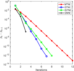
(a) Monotonically decreasing of $\bar{\rho}_{k}$
(Example 1)

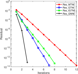
(b) Residuals (Example 1)

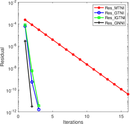
(c) Residuals (Example 2)

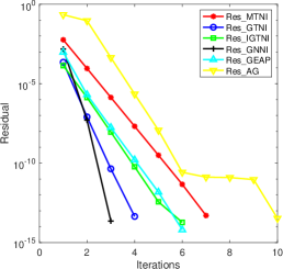
(d) Residuals (Example 3)

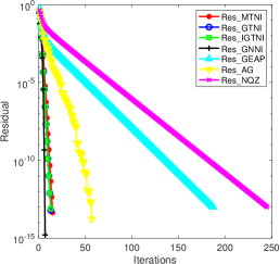
(e) Residuals (Example 4)

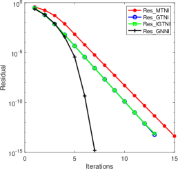
(f) Residuals (Example 4)

Figure 1: Results of Example 1,2,3,4

Table 1: Result of Example 1

method	$\lambda$	$\mathbf{x}$	Outer Iter	Inner Iter	Residual	Time(s)
MTNI	0.8774	[0.6028, 0.5234, 0.6023]	12	17086	1.9082e-14	0.7588
GTNI	0.8774	[0.6028, 0.5234, 0.6023]	7	1096	1.9347e-14	0.0757
IGTNI	0.8774	[0.6028, 0.5234, 0.6023]	8	1184	5.0898e-14	0.0684
GNNI	0.8774	[0.6028, 0.5234, 0.6023]	3	/	8.3544e-14	0.0115

Table 2: Result of Example 2

method	$\lambda$	Outer Iter	Inner Iter	Residual	Time(s)
MTNI	0.9859	16	41600	4.0477e-11	161.4059
GTNI	0.9859	3	6860	1.6140e-12	25.5504
IGTNI	0.9859	3	6137	3.5401e-12	22.3650
GNNI	0.9859	2	/	3.1140e-12	6.5572

Table 3: Result of Example 3

method	$\lambda$	Outer Iter	Inner Iter	Residual	Time(s)
MTNI	0.6712	7	19475	5.0431e-14	0.9461
GTNI	0.6712	4	379	4.4267e-14	0.0443
IGTNI	0.6712	6	400	1.8631e-14	0.0366
GNNI	0.6712	3	/	2.2748e-14	0.0083
GEAP	0.6712	6	/	6.4047e-15	0.0074
AG	0.6712	10	/	3.3375e-14	0.0042

Table 4: Result of Example 4

method	$\lambda$	Outer Iter	Inner Iter	Residual	Time(s)
MTNI	51.7310	15	6189	4.2891e-14	24.6596
GTNI	51.7310	13	5650	6.0176e-14	21.8478
IGTNI	51.7310	13	4432	7.7549e-14	17.0098
GNNI	51.7310	7	/	1.5861e-15	0.4592
GEAP	51.7310	187	/	9.8886e-14	1.4453
AG	51.7310	57	/	1.6767e-14	1.1369
NQZ	51.7310	245	/	9.8212e-14	0.9080

5.4 Computing the positive eigenpair for nonlinear eigenvalue problem with eigenvector nonlinearity (NEPv)

In this part, We consider to apply our methods on the nonlinear eigenvalue problem with eigenvector nonlinearity (NEPv) and compare the numerical results with other methods. The NEPv is originated from the Bose-Einstein condensates (BECs), which can be regarded as a special case of tensor generalized eigenvalue problem.

In condensed matter physics, a Bose–Einstein condensate (BEC) is a state of matter that is typically formed when a gas of bosons at very low densities is cooled to temperatures very close to absolute zero. Under such conditions, a large fraction of bosons occupy the same quantum ground state. Suppose that this ground state can be represented by a wave function $\psi(\mathbf{x},t)$. Then $\psi$ is the solution of the following energy functional minimization problem under normalization constraints [2, page 10]:

$$\left\{\begin{aligned} &\min~{}E\big{(}\psi(\cdot,t)\big{)}=\int_{\mathbb{R}^{d}}\big{[}\frac{1}{2}|\nabla\psi(\mathbf{x},t)|^{2}+V(\mathbf{x}|\psi(\mathbf{x},t)|^{2})+\frac{\beta}{2}|\psi(\mathbf{x},t)|^{4}\big{]}d\mathbf{x},\\ &~{}\mathrm{s.t.}\int_{\mathbb{R}^{d}}|\psi(\mathbf{x},t)|^{2}d\mathbf{x}=1,~{}E\big{(}\psi(\mathbf{x},t)\big{)}<\infty,\\ \end{aligned}\right.$$ (5.1)

where $\mathbf{x}\in\mathbb{R}^{d}$ is the spatial coordinate vector ($d=1,2,3$), $V(\mathbf{x})$ is an external trapping potential, and the given real constant $\beta$ is the dimensionless interaction coefficient, see [2, page 12].

The equation governing the motion of the condensate can be derived by [2, 31]

$$\left\{\begin{aligned} &\text{\i}\partial_{t}\psi(\mathbf{x},t)=-\frac{1}{2}\Delta\psi(\mathbf{x},t)+V(\mathbf{x})\psi(\mathbf{x},t)+\beta|\psi(\mathbf{x},t)|^{2}\psi(\mathbf{x},t),\\ &\int_{\mathbb{R}^{d}}|\psi(\mathbf{x},t)|^{2}d\mathbf{x}=1,\\ \end{aligned}\right.$$ (5.2)

which is a nonlinear Schrödinger equation (NLSE) with cubic nonlinearity, known as the Gross-Pitaevskii equation (GPE). Here “ı” denotes the imaginary unit.

Using the finite difference discretization [3], one-dimensional case of the BEC problem (5.1) can be transformed into a nonconvex quartic optimization problem over a spherical constraint:

$$\left\{\begin{aligned} &\min\limits_{\mathbf{u}\in\mathbb{R}^{N-2}}\frac{\alpha}{2}\sum\limits_{i=1}^{N-2}u_{i}^{4}+\mathbf{u}^{\top}B\mathbf{u},\\ &\mathrm{s.t.}~{}\|\mathbf{u}\|_{2}^{2}=1,\\ \end{aligned}\right.$$ (5.3)

where $\alpha=\beta/h$, $h=(b-a)/(N-1)$, $[a,b]$ is the computational domain, and $N$ is the total number of partition points on $[a,b]$. The vector $\mathbf{u}=\sqrt{h}\Psi$, where $\Psi=(\psi_{2},\ldots,\psi_{N-1})^{\top}$ and $\psi_{j}$ is the numerical approximation of $\psi$ on the partition point $x_{j}\in[a,b]$ for $j=1,\ldots,N$. The elements of $B=(b_{jk})\in\mathbb{R}^{(N-2)\times(N-2)}$ are given by

$$b_{jk}=\left\{\begin{aligned} &\frac{1}{h^{2}}+V(x_{j}),&j=k,\\ &-\frac{1}{2h^{2}},&|j-k|=1,\\ &0,&\text{otherwise}.\\ \end{aligned}\right.$$

Wu et al. [52] and Tian et al. [51] used Newton methods to compute the ground states of BECs. Huang et al. [32, section 3] mentioned that the optimization problem (5.3) is equivalent to the nonlinear eigenvalue problem

$$\left\{\begin{aligned} &\alpha\operatorname{\mathcal{A}}\mathbf{u}^{3}+B\mathbf{u}=\lambda\mathbf{u},\\ \ &\|\mathbf{u}\|^{2}=1,\\ \end{aligned}\right.$$ (5.4)

where $\operatorname{\mathcal{A}}$ equals to the unit tensor $\mathcal{I}$. According to [32, Lemma 1], there exists a unique eigenpair $(\lambda,\mathbf{u})$ with $\mathbf{u}>0$, and $\lambda>0$ is the smallest eigenvalue of NEPv (5.4).

Recall that the definition of the identity tensor $\mathcal{E}$ is $\mathcal{E}\mathbf{x}^{m-1}=\|\mathbf{x}\|^{m-2}\mathbf{x}$ for all $\mathbf{x}\in\mathbb{R}^{n}$. Using this definition, we can rewrite (5.4) as

$$\left\{\begin{aligned} &\mathcal{E}\mathbf{u}^{3}=\frac{1}{\lambda}(\alpha\operatorname{\mathcal{A}}+\mathcal{E}\times_{1}B)\mathbf{u}^{3},\\ &\|\mathbf{u}\|_{2}^{2}=1,\\ \end{aligned}\right.$$ (5.5)

which is a generalized eigenvalue problem for the tensor pair $(\mathcal{E},\alpha\operatorname{\mathcal{A}}+\mathcal{E}\times_{1}B)$. Multiplying both sides by a constant $c=\max\limits_{j}b_{jj}$, (5.5) becomes

$$\left\{\begin{aligned} &c\mathcal{E}\mathbf{u}^{3}=\frac{c}{\lambda}(\alpha\operatorname{\mathcal{A}}+\mathcal{E}\times_{1}B)\mathbf{u}^{3},\\ &||\mathbf{u}||_{2}^{2}=1.\\ \end{aligned}\right.$$ (5.6)

Obviously, the tensor $c\mathcal{E}$ is nonnegative and weakly irreducible. When $\beta$ is large enough, there exists a vector $\mathbf{v}\in\mathbb{R}^{N-2}$ satisfying $\mathbf{v}>0$ such that $(\alpha\operatorname{\mathcal{A}}+\mathcal{E}\times_{1}B)\mathbf{v}^{3}>c\mathcal{E}\mathbf{v}^{3}$. For any $(i_{2},i_{3},i_{4})\neq(i,i,i)$, we can easily see that

$$(\alpha\operatorname{\mathcal{A}}+\mathcal{E}\times_{1}B)_{i,i_{2},i_{3},i_{4}} =\sum\limits_{j}e_{ji_{2}i_{3}i_{4}}b_{ij}=b_{ii}e_{ii_{2}i_{3}i_{4}}+\sum\limits_{j\neq i}e_{ji_{2}i_{3}i_{4}}b_{ij}$$

$$\leq b_{ii}e_{ii_{2}i_{3}i_{4}}\leq ce_{ii_{2}i_{3}i_{4}}=(c\mathcal{E})_{ii_{2}i_{3}i_{4}}.$$

Therefore the tensor pair $(c\mathcal{E},\alpha\operatorname{\mathcal{A}}+\mathcal{E}\times_{1}B)$ is a generalized $\mathcal{M}$-tensor pair and hence the unique eigenpair $(\frac{c}{\lambda},\mathbf{u})$ can be computed by our algorithms.

Example 5 [31, Example 1] Consider the finite difference approximation with a grid size $h=2L/(N+1)$ of (5.2) with Dirichlet boundary conditions on $[-L,L]\times[-L,L]$, where $L>0$ is large enough, i.e.,

$$\frac{\beta}{h^{2}}\operatorname{diag}(\mathbf{u}^{[2]})\mathbf{u}+B\mathbf{u}=\lambda\mathbf{u},~{}\mathbf{u}^{\top}\mathbf{u}=1,$$

where $\mathbf{u}\in\mathbb{R}^{n}$, $n=N^{2}$. The matrix $B=A+V$ where $A=I\otimes L_{h}+L_{h}\otimes I$ is a negative 2D Laplacian matrix with

$$L_{h}=\frac{1}{h^{2}}\begin{bmatrix}2&-1&&&\\ -1&2&-1&&\\ &\ddots&\ddots&\ddots&\\ &&-1&2&-1\\ &&&-1&2\\ \end{bmatrix}\in\mathbb{R}^{N\times N}$$

and $V=h^{2}\operatorname{diag}(1^{2}+1^{2},1^{2}+2^{2},\ldots,N^{2}+N^{2})$ is the discretization of the harmonic potential $V(x,y)=x^{2}+y^{2}$. We compare our method GNNI with the Newton-Root-Finding Iteration (NRI) [31] and the Newton-Noda Iteration (NNI) for NEPv [31, 22] in this example. For NNI, the linear system in each iteration can be ill-conditioned and is hard to solve without an appropriate preconditioner. Therefore, we use MATLAB function ‘bicgstab’ to solve the linear system with tolerance as $10^{-9}$ and maximum iteration number as 200. For GNNI, the linear systems can be solved directly by MATLAB function ‘mldivide’ (‘$\backslash$’) but we found that using ‘bicgstab’ is faster when $n$ is relatively large. So we use ‘bicgstab’ only on large examples for this method. For NRI, the linear system in the inner iterations has a tridiagonal (or block tridiagonal) structure, so we can solve it efficiently by the block tridiagonal LU factorization. In addition, the NRI method needs an initial interval $[a,b]$ for $\lambda$, we regard the initial $\lambda$ as known constants for this method in our experiments.

The identity tensor $\mathcal{E}\in T_{4,n}$ can be generated by [34, Property 2.4]

$$e_{i_{1}i_{2}i_{3}i_{4}}=\frac{1}{4!}\sum\limits_{p\in\Pi_{4}}\delta_{i_{p(1)}i_{p(2)}}\delta_{i_{p(3)}i_{p(4)}}$$ (5.7)

for $i_{1},i_{2},i_{3},i_{4}\in\{1,\ldots,n\}$, where $\delta$ is the standard Kronecker delta, i.e., $\delta_{ij}=1$ if $i=j$ and $\delta_{ij}=0$ if $i\neq j$. The results are shown in Table 5.

Table 5: Result of Example 5

$n=15^{2}$, $\beta=100000$, $L=8$
method	$\lambda$	Outer Iter	Inner Iter	Residual	Time(s)
GNNI	610.0432	5	/	3.5411e-13	0.0090
NRI	610.0432	3	[12,13,13]	2.2609e-13	0.0465
NNI	610.0432	5	/	2.4747e-12	0.0301
$n=63^{2}$, $\beta=200000$, $L=8$
method	$\lambda$	Outer Iter	Inner Iter	Residual	Time(s)
GNNI	976.5971	4	/	1.9504e-12	1.9694
NRI	976.5971	3	[16,16,16]	4.1177e-13	4.8632
NNI	976.5971	4	/	6.8873e-13	2.3075
$n=99^{2}$, $\beta=200000$, $L=8$
method	$\lambda$	Outer Iter	Inner Iter	Residual	Time(s)
GNNI	968.5025	4	/	2.7739e-12	18.0728
NRI	968.5025	3	[18,18,18]	6.0493e-13	34.7647
NNI	968.5025	4	/	1.0452e-12	19.4114

Example 6 [22, Example 3] Consider the modified Gross-Pitaevskii equation (MGPE)

$$A\mathbf{u}+V\mathbf{u}+\frac{\beta}{h^{2}}\mathbf{u}^{[3]}+2\frac{\alpha}{h^{2}}A\mathbf{u}^{[3]}=\lambda\mathbf{u},~{}\mathbf{u}^{\top}\mathbf{u}=1$$ (5.8)

with an optical potential $V(x,y)=\frac{1}{2}(x^{2}+y^{2})+40\big{(}\sin^{2}(\frac{\pi x}{2})+\sin^{2}(\frac{\pi y}{2})\big{)}$ on the domain $[-2,2]^{2}$, where $A=\frac{1}{2}(I\otimes L_{h}+L_{h}\otimes I)$. This equation can also be rewritten into a tensor generalized eigenvalue problem

$$\left\{\begin{aligned} &c\mathcal{E}\mathbf{u}^{3}=\frac{c}{\lambda}\big{(}2\frac{\alpha}{h^{2}}\mathcal{I}\times_{1}A+\frac{\beta}{h^{2}}\mathcal{I}+\mathcal{E}\times_{1}(A+V)\big{)}\mathbf{u}^{3},\\ &\|\mathbf{u}\|_{2}^{2}=1,\\ \end{aligned}\right.$$

where $c$ is a positive constant. Denote $\mathcal{A}=c\mathcal{E}$, $\mathcal{B}=2\frac{\alpha}{h^{2}}\mathcal{I}\times_{1}A+\frac{\beta}{h^{2}}\mathcal{I}+\mathcal{E}\times_{1}(A+V)$ and let $c=\max\big{(}\operatorname{diag}(A+V)\big{)}$, then we can easily see that $b_{ii_{2}i_{3}i_{4}}\leq a_{ii_{2}i_{3}i_{4}}$ for any $i=1,\ldots,n$ and $(i_{2},i_{3},i_{4})\neq(i,i,i)$. Besides, there exsits a vector $\mathbf{v}>0$ such that $(\operatorname{\mathcal{B}}-\operatorname{\mathcal{A}})\mathbf{v}^{3}>0$ when $\beta$ is large enough. Therefore, the MGPE also satisfies our assumptions and the unique positive eigenpair of (5.8) can be found by our methods. We compare the GNNI method with the NNI method [22] in this example, the results are shown in Table 6.

Table 6: Result of Example 6

$n=63^{2}$, $\beta=100000$, $\alpha=100$, $L=2$
method	$\lambda$	Outer Iter	Inner Iter	Residual	Time(s)
GNNI	7.9343e+03	6	/	1.7693e-11	3.5730
NNI	7.9343e+03	4	/	7.6481e-11	3.6068

6 Conclusions

In this paper, the Noda iteration(NI) method has been developed for computing the Perron pair for the generalized $\mathcal{M}$-tensor pair. We prove that MTNI, GTNI, IGTNI, and GNNI are convergent based on the techniques in [13, 21, 39, 55]. We test our methods on randomly generated tensor pairs, hypergraph eigenproblem as well as NEPv and the convergence on accuracy was illustrated. Acceleration of the methods may be a topic of future study. Specifically, we need to develop a faster method for solving the $\mathcal{M}$-tensor equation $(\rho_{k-1}\operatorname{\mathcal{B}}-\operatorname{\mathcal{A}})\mathbf{y}_{k}^{m-1}=(\operatorname{\mathcal{B}}-\operatorname{\mathcal{A}})\mathbf{x}_{k-1}^{m-1}$ and the choice of parameter $\varepsilon$ needs to be dicussed. For Algorithm 4, other ways for choosing the step size and some variations of Newton method need to be considered. In view of Algorithm 1 and Algorithm 2, another work that needs to be done is to consider a more general iteration formula as $(\rho_{k-1}\operatorname{\mathcal{B}}-\operatorname{\mathcal{A}})\mathbf{y}_{k}^{m-1}=(\alpha_{k-1}\operatorname{\mathcal{A}}+\beta_{k-1}\operatorname{\mathcal{B}})\mathbf{x}_{k-1}^{m-1}$. As we can see from the numerical experiments, Algorithm 2 performs faster than Algorithm 1. How to choose $\alpha_{k-1}$, $\beta_{k-1}$ in each iteration to make the method more efficient needs further discussion.

Appendix (MATLAB codes)

In order to run the following codes correctly, the Tensor Toolbox [1] needs to be added to the path.

ExampleGenerator.m

%% Example 1 (random 3x3x3)

m = 3;

n = 3;

I = tenzeros(n$*$ones(1,m));

for i = 1:n

I(i$*$ones(1,m)) = 1;

end

R = tenrand(n$*$ones(1,m));

epsilon = 0.01;

c = (1 + epsilon) $*$ max(ttsv(R,ones(n,1),-1));

C = c $*$ I - R;

A = tenrand(n$*$ones(1,m));

B = A + C;

save(’A(example 1 random 3x3x3).mat’,’A’);

save(’B(example 1 random 3x3x3).mat’,’B’);

%% Example 2 (random 50x50x50x50)

m = 4;

n = 50;

I = tenzeros(n$*$ones(1,m));

for i = 1:n

I(i$*$ones(1,m)) = 1;

end

R = tenrand(n$*$ones(1,m));

epsilon = 0.01;

c = (1 + epsilon) $*$ max(ttsv(R,ones(n,1),-1));

C = c $*$ I - R;

A = tenrand(n$*$ones(1,m));

B = A + C;

save(’A(example 2 random 50x50x50x50).mat’,’A’);

save(’B(example 2 random 50x50x50x50).mat’,’B’);

%% Example 3 (random 4x4x4x4x4x4 symmetric)

m = 6;

n = 4;

R = rand(n$*$ones(1,m));

R = tensor(symtensor(tensor(round(R,4))));

I = tenzeros(size(R));

for i = 1:n

I(i$*$ones(1,m)) = 1;

end

A = rand(n$*$ones(1,m));

A = tensor(symtensor(tensor(round(A,4))));

gamma = max([1.01 $*$ max(ttsv(R,ones(n,1),-1)),max( R(:)-A(:))$*$n^(m-1)]);

B = gamma $*$ I - R + A;

save(’A(example 3 random 4x4x4x4x4x4 symmetric).mat’,’A’);

save(’B(example 3 random 4x4x4x4x4x4 symmetric).mat’,’B’);

%% Example 4 (hypergraph 50x50x50x50)

m = 4;

n = 50;

omega = 1;

D = tenzeros(n$*$ones(1,m));

for i = 1:5

D(i$*$ones(1,m)) = n - 2 -i;

end

D(6$*$ones(1,m)) = 12;

D(7$*$ones(1,m)) = 14;

for i = 8:n-2

D(i$*$ones(1,m)) = 15;

end

D((n-1)$*$ones(1,m)) = 10;

D(n$*$ones(1,m)) = 5;

C = tenzeros(n$*$ones(1,m));

for i1 = 1:5

for i2 = i1+1:n-2

C(i1,i2,i2+1,i2+2) = factorial(m) / factorial(m-1);

end

end

C = tensor(symtensor(C));

A = omega $*$ D + C;

I = zeros(n$*$ones(1,m));

for i = 1:n

I(i,i,i,i) = 1;

end

B = tensor(100 $*$ I);

save(’A(example 4 hypergraph 50x50x50x50).mat’,’A’);

save(’B(example 4 hypergraph 50x50x50x50).mat’,’B’);

%% Example 5 (Nonlinear eigenvalue–2D case)

m = 4;

N = 15;

n = N^2;

L = 8;

h = 2$*$L / (N+1);

beta = 100000;

beta = beta / h^2;

L = 1/h^2 $*$ (2$*$eye(N)-diag(ones(N-1,1),1)-diag(ones(N-1,1),-1));

V = zeros(n,n);

for i = 1:N

for j = 1:N

V((i-1)$*$N+j,(i-1)$*$N+j) = h^2 $*$ (i^2+j^2);

end

end

A = kron(eye(N),L)+kron(L,eye(N));

B = A + V;

kappa = sqrt(norm(A,1)*norm(A,inf)) + beta;

save(’data(example 5 NEPv).mat’,’A’,’B’,’beta’,’m’,’n’,’kappa’);

%% Example 6 (Nonlinear eigenvalue–MGPE)

m = 4;

N = 63;

n = N^2;

L = 2;

h = 2$*$L / (N+1);

beta = 100000;

beta = beta / h^2;

alpha = 100;

alpha = alpha / h^2;

L = 1/h^2 $*$ (2$*$eye(N)-diag(ones(N-1,1),1)-diag(ones(N-1,1),-1));

V = zeros(n,n);

for i = 1:N

for j = 1:N

V((i-1)$*$N+j,(i-1)$*$N+j) = 1/2 $*$ (i^2+j^2) + 40 $*$ (sin(pi$*$i/2)^2+sin(pi$*$j/2)^2);

end

end

A = 1/2 $*$ (kron(eye(N),L)+kron(L,eye(N)));

B = A + V;

kappa = sqrt(norm(A,1)$*$norm(A,inf)) + beta;

save(’data(example 6 MGPE).mat’,’A’,’B’,’beta’,’m’,’n’,’kappa’);

MTNI.m

clearvas;

clc;

%% Generate Examples

%% Example 1

load(”A(example 1 random 3x3x3).mat”);

load(”B(example 1 random 3x3x3).mat”);

%% Example 2

% load(”A(example 2 random 50x50x50x50).mat”);

% load(”B(example 2 random 50x50x50x50).mat”);

%% Example 3 (random 4x4x4x4x4x4 symmetric)

% load(”A(example 3 random 4x4x4x4x4x4 symmetric).mat”);

% load(”B(example 3 random 4x4x4x4x4x4 symmetric).mat”);

%% Example 4 (hypergraph 50x50x50x50)

% load(”A(example 4 hypergraph 50x50x50x50).mat”);

% load(”B(example 4 hypergraph 50x50x50x50).mat”);

%% Initialization

tic;

m = length(size(A));

N = size(A);

n = N(1);

tol = 1e-13;

C = double(B - A);

D = zeros(n$*$ones(1,m));

d = zeros(n,1);

for i = 1 : n

d(i) = C(i,i,i); % for m=3

%    d(i) = C(i,i,i,i); % for m=4

D(i,i,i) = d(i); % for m=3

%    D(i,i,i,i) = d(i); % for m=4

end

b = ones(n,1);

x = ones(n,1);

x_old = x;

Temp = tensor(D - C);

C = tensor(C);

b_temp = double(ttsv(Temp,x,-1)) + b;

x_new = (b_temp ./ d) .^ (1/(m-1));

while norm(x_new - x_old,2) $>$ tol

x_old = x_new;

b_temp = double(ttsv(Temp,x_old,-1)) + b;

x_new = (b_temp ./ d) .^ (1/(m-1));

end

x = x_new / norm(x_new,2);

temp1 = ttsv(A,x,-1);

temp2 = ttsv(B,x,-1);

temp3 = temp2 - temp1;

rho_max = max(temp1 ./ temp2);

rho = rho_max;

y = ones(n,1);

%%

epsilon = 0.01; % for example 1,4

% epsilon = 0.005; % for example 2,3

delta = 1e-13; % for example 1,3

% delta = 1e-15; % for example 2,4

d = zeros(n,1);

MaxIter = 50;

Differ_rho = zeros(1,MaxIter);

Res_rho = zeros(1,MaxIter);

Res = zeros(1,MaxIter);

count = zeros(1,MaxIter);

for k = 1 : MaxIter

M = double(rho $*$ B - A);

D = zeros(n$*$ones(1,m));

for i = 1 : n

d(i) = M(i,i,i); % for m=3

%        d(i) = M(i,i,i,i); % for m=4

D(i,i,i) = d(i); % for m=3

%        D(i,i,i,i) = d(i); % for m=4

end

y_old = y;

r = temp3;

Temp = tensor(D - M);

b_temp = ttsv(Temp,y_old,-1) + r;

y_new = (b_temp ./ d) .^ (1/(m-1));

count(k) = 0;

while norm(y_new - y_old,2) $>$ delta

y_old = y_new;

b_temp = ttsv(Temp,y_old,-1) + r;

y_new = (b_temp ./ d) .^ (1/(m-1));

count(k) = count(k) + 1;

if count(k) $>=$ 3000 && k == 1

break;

end

end

y = y_new;

rho_old = rho_max;

tau = min(temp3 ./ ttsv(C,y,-1));

rho = rho - (1 - rho) $*$ tau / (1 - tau);

rho = (1 + epsilon) $*$ rho;

x = y / norm(y,2);

temp1 = ttsv(A,x,-1);

temp2 = ttsv(B,x,-1);

temp3 = temp2 - temp1;

s_max = max(temp1 ./ temp3);

rho_max = s_max / (1 + s_max);

s_min = min(temp1 ./ temp3);

rho_min = s_min / (1 + s_min);

Differ_rho(k) = rho_old - rho_max;

Res_rho(k) = abs(rho_max-rho_min)/rho_max;

Res(k) = norm(temp1-rho_max$*$temp2,2);

%    if Res(k) $<$ tol % for symmetric case

%        break;

%    end

if Res_rho(k) $<$ tol

break;

end

end

time=toc;

GTNI.m

clearvas;

clc;

%% Generate Examples

%% Example 1

load(”A(example 1 random 3x3x3).mat”);

load(”B(example 1 random 3x3x3).mat”);

%% Example 2

% load(”A(example 2 random 50x50x50x50).mat”);

% load(”B(example 2 random 50x50x50x50).mat”);

%% Example 3 (random 4x4x4x4x4x4 symmetric)

% load(”A(example 3 random 4x4x4x4x4x4 symmetric).mat”);

% load(”B(example 3 random 4x4x4x4x4x4 symmetric).mat”);

%% Example 4 (hypergraph 50x50x50x50)

% load(”A(example 4 hypergraph 50x50x50x50).mat”);

% load(”B(example 4 hypergraph 50x50x50x50).mat”);

%% Initialization

tic;

m = length(size(A));

N = size(A);

n = N(1);

tol = 1e-13;

x = ones(n,1);

x = x / norm(x,2);

temp1 = ttsv(A,x,-1);

temp2 = ttsv(B,x,-1);

rho_max = max(temp1 ./ temp2);

rho_min = min(temp1 ./ temp2);

rho = 1;

y = ones(n,1);

%%

delta = 1e-13; % for example 1,2

%delta = 1e-15; % for example 3,4

d = zeros(n,1);

MaxIter = 50;

Differ_rho = zeros(1,MaxIter);

Res_rho = zeros(1,MaxIter);

Res = zeros(1,MaxIter);

count = zeros(1,MaxIter);

Epsilon = zeros(1,MaxIter);

for k = 1 : MaxIter

M = double(rho $*$ B - A);

D = zeros(n$*$ones(1,m));

for i = 1 : n

d(i) = M(i,i,i); % for m=3

%        d(i) = M(i,i,i,i); % for m=4

D(i,i,i) = d(i); % for m=3

%        D(i,i,i,i) = d(i); % for m=4

end

y_old = y;

r = temp1;

Temp = tensor(D - M);

b_temp = ttsv(Temp,y_old,-1) + r;

y_new = (b_temp ./ d) .^ (1/(m-1));

count(k) = 0;

while norm(y_new - y_old,2)$>$delta

y_old = y_new;

b_temp = ttsv(Temp,y_old,-1) + r;

y_new = (b_temp ./ d) .^ (1/(m-1));

count(k) = count(k) + 1;

end

y = y_new;

Epsilon(k) = 1;

%    Epsilon(k) = 0.01; % for example 4

temp = 1-min(temp1./(ttsv(A,y,-1)+temp1));

while 1

if (1+Epsilon(k)) $*$ temp $<=$ 1

break;

else

Epsilon(k) = Epsilon(k)/2;

end

end

epsilon = Epsilon(k);

rho = (1+epsilon) $*$ rho $*$ temp;

x = y / norm(y,2);

temp1 = ttsv(A,x,-1);

temp2 = ttsv(B,x,-1);

rho_old = rho_max;

rho_max = max(temp1 ./ temp2);

rho_min = min(temp1 ./ temp2);

Differ_rho(k) = rho_old - rho_max;

Res_rho(k) = abs(rho_max-rho_min)/rho_max;

Res(k) = norm(temp1-rho_max$*$temp2,2);

%    if Res(k) $<$ tol % for symmetric case

%        break;

%    end

if Res_rho(k) $<$ tol

break;

end

end

time=toc;

IGTNI.m

clearvas;

clc;

%% Generate Examples

%% Example 1

load(”A(example 1 random 3x3x3).mat”);

load(”B(example 1 random 3x3x3).mat”);

%% Example 2

% load(”A(example 2 random 50x50x50x50).mat”);

% load(”B(example 2 random 50x50x50x50).mat”);

%% Example 3 (random 4x4x4x4x4x4 symmetric)

% load(”A(example 3 random 4x4x4x4x4x4 symmetric).mat”);

% load(”B(example 3 random 4x4x4x4x4x4 symmetric).mat”);

%% Example 4 (hypergraph 50x50x50x50)

% load(”A(example 4 hypergraph 50x50x50x50).mat”);

% load(”B(example 4 hypergraph 50x50x50x50).mat”);

%% Initialization

tic;

m = length(size(A));

N = size(A);

n = N(1);

tol = 1e-13;

x = ones(n,1);

x = x / norm(x,2);

temp1 = ttsv(A,x,-1);

temp2 = ttsv(B,x,-1);

rho_max = max(temp1 ./ temp2);

rho_min = min(temp1 ./ temp2);

rho = 1;

y = ones(n,1);

%%

d = zeros(n,1);

MaxIter = 50;

Differ_rho = zeros(1,MaxIter);

Res_rho = zeros(1,MaxIter);

Res = zeros(1,MaxIter);

count = zeros(1,MaxIter);

gama = zeros(1,MaxIter);

f = zeros(1,MaxIter);

Epsilon= zeros(1,MaxIter);

for k = 1 : MaxIter

M = double(rho $*$ B - A);

D = zeros(n$*$ones(1,m));

for i = 1 : n

d(i) = M(i,i,i); % for m=3

%        d(i) = M(i,i,i,i); % for m=4

D(i,i,i) = d(i); % for m=3

%        D(i,i,i,i) = d(i); % for m=4

end

y_old = y;

r = temp1;

gama(k) = min((rho_max-rho_min)/rho_max,1e-3);

f(k) = max(gama(k)$*$min(r),1e-12);

Temp = tensor(D - M);

b_temp = ttsv(Temp,y_old,-1) + r + f(k);

y_new = (b_temp ./ d) .^ (1/(m-1));

count(k) = 0;

while norm(y_new-y_old,2) $>$ 1e-13 % for example 1,4

%    while norm(y_new-y_old,2) $>$ 1e-12 % for example 2

%    while norm(y_new-y_old,2) $>$ 1e-14 % for example 3

y_old = y_new;

b_temp = ttsv(Temp,y_old,-1) + r + f(k);

y_new = (b_temp ./ d) .^ (1/(m-1));

count(k) = count(k) + 1;

end

y = y_new;

Epsilon(k) = 1;

%    Epsilon(k) = 0.01; % for example 4

temp = 1-min((temp1+f(k))./(ttsv(A,y,-1)+temp1+f(k)));

while 1

if (1+Epsilon(k)) $*$ temp $<=$ 1

break;

else

Epsilon(k) = Epsilon(k)/2;

end

end

epsilon = Epsilon(k);

rho = (1+epsilon) $*$ rho $*$ temp;

x = y / norm(y,2);

temp1 = ttsv(A,x,-1);

temp2 = ttsv(B,x,-1);

rho_old = rho_max;

rho_max = max(temp1 ./ temp2);

rho_min = min(temp1 ./ temp2);

Differ_rho(k) = rho_old - rho_max;

Res_rho(k) = abs(rho_max-rho_min)/rho_max;

Res(k) = norm(temp1-rho_max$*$temp2,2);

%    if Res(k) $<$ tol % for symmetric case

%        break;

%    end

if Res_rho(k) $<$ tol

break;

end

end

time = toc;

GNNI.m

clearvas;

clc;

%% Load Examples

%% Example 1

load(”A(example 1 random 3x3x3).mat”);

load(”B(example 1 random 3x3x3).mat”);

m = length(size(A));

N = size(A);

n = N(1);

for i = 1:n

A(i,:,:) = tensor(symtensor(A(i,:,:)));

B(i,:,:) = tensor(symtensor(B(i,:,:)));

end

%% Example 2

% load(”A(example 2 random 50x50x50x50).mat”);

% load(”B(example 2 random 50x50x50x50).mat”);

% m = length(size(A));

% N = size(A);

% n = N(1);

% for i = 1:n

%    A(i,:,:,:) = tensor(symtensor(A(i,:,:,:)));

%    B(i,:,:,:) = tensor(symtensor(B(i,:,:,:)));

% end

%% Example 3 (random 4x4x4x4x4x4 symmetric)

% load(”A(example 3 random 4x4x4x4x4x4 symmetric).mat”);

% load(”B(example 3 random 4x4x4x4x4x4 symmetric).mat”);

% m = length(size(A));

% N = size(A);

% n = N(1);

%% Example 4 (hypergraph 50x50x50x50)

% load(”A(example 4 hypergraph 50x50x50x50).mat”);

% load(”B(example 4 hypergraph 50x50x50x50).mat”);

% m = length(size(A));

% N = size(A);

% n = N(1);

%% Initialization

tic;

tol = 1e-13;

C = double(B - A);

D = zeros(n$*$ones(1,m));

d = zeros(n,1);

for i = 1 : n

d(i) = C(i,i,i); % for m=3

%    d(i) = C(i,i,i,i); % for m=4

D(i,i,i) = d(i); % for m=3

%    D(i,i,i,i) = d(i); % for m=4

end

b = ones(n,1);

x = ones(n,1);

x_old = x;

Temp = tensor(D - C);

C = tensor(C);

b_temp = double(ttsv(Temp,x,-1)) + b;

x_new = (b_temp ./ d) .^ (1/(m-1));

while norm(x_new - x_old,2) $>$ tol

x_old = x_new;

b_temp = double(ttsv(Temp,x_old,-1)) + b;

x_new = (b_temp ./ d) .^ (1/(m-1));

end

x = x_new / norm(x_new,2);

T = double(ttsv(A,x,-2));

T_B = double(ttsv(B,x,-2));

temp1 = T $*$ x;

temp2 = T_B $*$ x;

rho = max(temp1 ./ temp2);

%%

MaxIter = 50;

Differ_rho = zeros(1,MaxIter);

Res_rho = zeros(1,MaxIter);

Res = zeros(1,MaxIter);

R = zeros(MaxIter,n);

theta = zeros(1,MaxIter);

for k = 1: MaxIter

M = rho $*$ B - A;

b = temp2;

J_x = (m - 1) $*$ (rho $*$ T_B - T);

w = J_x $\backslash$ b;

y = w / norm(w,2);

theta(k) = 1;

while 1

x_new = (m-2) $*$ x + theta(k) $*$ y;

r = abs(ttsv(M,x_new,-1));

R(k,1:n) = r - theta(k) $*$ b / (2$*$norm(w)); % m=3

%        R(k,1:n) = r - theta(k) $*$ b / (norm(w)); % m$>=$4

if R(k,1:n)$>=$0 & ttsv(C,x_new,-1)$>$0

break;

else

theta(k) = theta(k)/2;

end

end

x = x_new / norm(x_new,2);

rho_old = rho;

T = double(ttsv(A,x,-2));

T_B = double(ttsv(B,x,-2));

temp1 = T $*$ x;

temp2 = T_B $*$ x;

rho_max = max(temp1 ./ temp2);

rho_min = min(temp1 ./ temp2);

rho = rho_max;

Differ_rho(k) = rho_old - rho;

Res_rho(k) = abs(rho_max-rho_min)/rho_max;

Res(k) = norm(temp1-rho_max$*$temp2,2);

if Res_rho(k) $<$ tol

break;

end

%    if Res(k) $<$ tol % for symmetric cases

%        break;

%    end

end

time = toc;

GNNI_NEPv.m (for Example 5)

clearvas;

clc;

%% Load Example

%% Example 5 (Nonlinear eigenvalue–2D case)

load(”data(example 5 NEPv).mat”);

bb = diag(B);

I = eye(n);

tt = max(bb);

%% Initialization

tic;

tol = 1e-13;

d = (beta - tt) $*$ ones(n,1) + diag(B);

b = ones(n,1);

x = ones(n,1);

x_old = x;

temp = x_old.^(m-1);

b_temp = bb .$*$ temp - tt $*$ temp - norm(x_old)^(m-2) $*$ (B $*$ x_old - tt $*$ x_old) + b;

x_new = (b_temp ./ d) .^ (1/(m-1));

while norm(x_new - x_old,2) $>$ 1e-1

x_old = x_new;

temp = x_old.^(m-1);

b_temp = bb .$*$ temp - tt $*$ temp - norm(x_old)^(m-2) $*$ (B $*$ x_old - tt $*$ x_old) + b;

x_new = (b_temp ./ d) .^ (1/(m-1));

end

x = x_new / norm(x_new,2);

temp1 = tt $*$ x;

temp2 = beta $*$ x.^(m-1) + B $*$ x;

rho = max(temp1 ./ temp2);

%%

MaxIter = 50;

Res_rho = zeros(MaxIter,1);

Res = zeros(MaxIter,1);

R = zeros(MaxIter,n);

theta = zeros(MaxIter,1);

for k = 1: MaxIter

b = temp2;

T = 1/3 $*$ I + 2/3 $*$ (x $*$ x’);

T_B = beta $*$ diag(x.^2) + 1/3$*$B + 2/3$*$(B$*$x)$*$x’;

T = tt $*$ T;

J_x = (m - 1) $*$ (rho $*$ T_B - T);

w = bicgstab(J_x,b,1e-9,200);

y = w / norm(w,2);

theta(k) = 1;

x_new = (m-2) $*$ x + theta(k) $*$ y;

x = x_new / norm(x_new,2);

rho_old = rho;

temp1 = tt $*$ x;

temp2 = beta $*$ x.^(m-1) + B $*$ x;

rho_max = max(temp1 ./ temp2);

rho_min = min(temp1 ./ temp2);

rho = rho_max;

Res_rho(k) = abs(rho_max-rho_min)/rho_max;

Res(k) = norm(temp1-rho_max$*$temp2,2);

if Res_rho(k) $<$ tol

break;

end

%    if Res(k) $<$ tol % for symmetric cases

%        break;

%    end

end

time = toc;

GNNI_MGPE.m (for Example 6)

clearvas;

clc;

%% Load Example

%% Example 6 (Nonlinear eigenvalue–MGPE)

load(”data(example 6 MGPE).mat”);

bb = diag(B);

tt = max(bb);

aa = diag(A);

I = eye(n);

Beta = beta $*$ I + 2 $*$ alpha $*$ A;

%% Initialization

tic;

tol = 1e-12;

d = (beta - tt) $*$ ones(n,1) + bb + 2 $*$ alpha $*$ aa;

x = ones(n,1);

x = x / norm(x);

temp1 = tt $*$ x;

temp2 = beta $*$ x.^(m-1) + 2$*$alpha$*$A$*$x.^(m-1) + B $*$ x;

rho = max(temp1 ./ temp2);

%%

MaxIter = 50;

Res_rho = zeros(1,MaxIter);

Res = zeros(1,MaxIter);

R = zeros(MaxIter,n);

theta = zeros(1,MaxIter);

for k = 1: MaxIter

b = temp2;

T_B = diag(beta$*$xx) + A.$*$repmat(2$*$alpha$*$xx’,n,1) + 1/3 $*$ B;

T_B = T_B + 2/3 $*$ (B$*$x) $*$ x’;

T = 1/3 $*$ tt $*$ I + 2/3 $*$ tt $*$ (x $*$ x’);

J_x = (m - 1) $*$ (rho $*$ T_B - T);

w = bicgstab(J_x,b,1e-9,200);

y = w / norm(w,2);

theta(k) = 1;

x_new = (m-2) $*$ x + theta(k) $*$ y;

x = x_new / norm(x_new,2);

rho_old = rho;

temp1 = tt $*$ x;

temp2 = beta $*$ x.^(m-1) + 2$*$alpha$*$A$*$x.^(m-1) + B$*$x;

rho_max = max(temp1 ./ temp2);

rho_min = min(temp1 ./ temp2);

rho = rho_max;

Res_rho(k) = abs(rho_max-rho_min)/rho_max;

Res(k) = norm(temp1-rho_max$*$temp2,2);

if Res_rho(k) $<$ tol

break;

end

%    if Res(k) $<$ tol % for symmetric cases

%        break;

%    end

end

time = toc;

Algorithms for comparison

GEAP.m

clearvas;

clc;

%% Load Examples

%% Example 3 (random 4x4x4x4x4x4 symmetric)

load(”A(example 3 random 4x4x4x4x4x4 symmetric).mat”);

load(”B(example 3 random 4x4x4x4x4x4 symmetric).mat”);

%% Example 4 (hypergraph 50x50x50x50)

% load(”A(example 4 hypergraph 50x50x50x50).mat”);

% load(”B(example 4 hypergraph 50x50x50x50).mat”);

%%

tic;

m = length(size(A));

N = size(A);

n = N(1);

x = ones(n,1);

x = x / norm(x,2);

temp1 = double(ttsv(A,x,-2));

temp2 = double(ttsv(B,x,-2));

temp3 = temp1 $*$ x;

temp4 = temp2 $*$ x;

temp5 = x’ $*$ temp3;

temp6 = x’ $*$ temp4;

beta = 1;

tau = 1e-6;

tol = 1e-13;

MaxIter = 50; % for example 3

% MaxIter = 200; % for example 4

Lambda = zeros(MaxIter,1);

H = zeros(n);

Alpha = zeros(MaxIter,1);

Res = zeros(MaxIter,1);

for k = 1 : MaxIter

Lambda(k) = temp5 / temp6;

H = m^2$*$temp5/(temp6)^3$*$2$*$(temp4$*$temp4’)+m/ temp6$*$((m-1)$*$temp1+temp5$*$(eye(n)

+(m-2)$*$(x$*$x’))+m$*$(temp3$*$x’+x$*$temp3’))-m/(temp6)^2$*$((m-1)$*$temp5$*$temp2

+m$*$(temp3$*$temp4’+temp4$*$temp3’)+m$*$temp5$*$(x$*$temp4’+temp4$*$x’));

e = eig(beta$*$H);

Alpha(k) = beta $*$ max(0,(tau-min(e))/m);

x = beta $*$ (temp3-Lambda(k)$*$temp4+(Alpha(k)+Lambda( k))$*$temp6$*$x);

x = x / norm(x,2);

temp1 = double(ttsv(A,x,-2));

temp2 = double(ttsv(B,x,-2));

temp3 = temp1 $*$ x;

temp4 = temp2 $*$ x;

temp5 = x’ $*$ temp3;

temp6 = x’ $*$ temp4;

Res(k) = norm(temp3-Lambda(k)$*$temp4,2);

if Res(k) $<$ tol

break;

end

end

lambda = Lambda(k);

time = toc;

AG.m

clearvas;

clc;

%% Load Examples

%% Example 3 (random 4x4x4x4x4x4 symmetric)

load(”A(example 3 random 4x4x4x4x4x4 symmetric).mat”);

load(”B(example 3 random 4x4x4x4x4x4 symmetric).mat”);

%% Example 4 (hypergraph 50x50x50x50)

% load(”A(example 4 hypergraph 50x50x50x50).mat”);

% load(”B(example 4 hypergraph 50x50x50x50).mat”);

%%

tic;

m = length(size(A));

N = size(A);

n = N(1);

x = ones(n,1);

x = x/norm(x,2);

Temp1 = ttsv(A,x,-1);

temp1 = x’ $*$ Temp1;

Temp2 = ttsv(B,x,-1);

temp2 = x’ $*$ Temp2;

rho = 0.001; % for example 3

% rho = 0.5; % for example 4

tol = 1e-13;

MaxIter = 50; % for example 3

% MaxIter = 100; % for example 4

Res = zeros(1,MaxIter);

for k = 1:MaxIter

lambda = temp1 / temp2;

g = m/temp2 $*$ (Temp1 - lambda$*$Temp2);

if k == 1

alpha = 1/norm(g);

else

alpha = min(1/norm(g),norm(x-x_old)/norm(g-g_old));

end

x_new = sqrt(1-alpha^2$*$norm(g)^2)$*$x+alpha$*$g;

count = 0;

while ttsv(A,x_new,0)/ttsv(B,x_new,0) $<$ lambda+rho$*$alpha$*$norm(g)^2

alpha = alpha / 2;

x_new = sqrt(1-alpha^2$*$norm(g)^2)$*$x+alpha$*$g;

count = count + 1;

%        if count $>=$ 2 % for example 4

%            break;

%        end

end

Res(k) = norm(Temp1 - lambda $*$ Temp2,2);

g_old = g;

x_old = x;

x = x_new;

Temp1 = ttsv(A,x,-1);

temp1 = x’ $*$ Temp1;

Temp2 = ttsv(B,x,-1);

temp2 = x’ $*$ Temp2;

lambda_old = lambda;

lambda = temp1 / temp2;

if Res(k) $<$ tol

break;

end

end

time = toc;

NQZ.m

clearvars;

clc;

%% Load Example

%% Example 4 (hypergraph 50x50x50x50)

load(”A(example 4 hypergraph 50x50x50x50).mat”);

m = length(size(A));

N = size(A);

n = N(1);

%%

tic;

x = ones(n,1);

x = x / norm(x,2);

y = double(ttsv(A,x,-1));

tol = 1e-13;

MaxIter = 300;

Res_rho = zeros(1,MaxIter);

Res = zeros(1,MaxIter);

for k = 1 : MaxIter

x = y.^(1/(m-1));

x = x / norm(x,2);

y = double(ttsv(A,x,-1));

lambda_ub = max(y ./ x.^(m-1));

lambda_lb = min(y ./ x.^(m-1));

lambda = lambda_ub;

Res_rho(k) = abs(lambda_ub - lambda_lb)/lambda_ub;

Res(k) = norm(y - lambda $*$ x.^(m-1));

if Res(k) $<$ tol

break;

end

end

time = toc;

NNI_NEPv.m (for Example 5)

clearvars;

clc;

%% Load Example

%% Example 5 (Nonlinear eigenvalue–2D case)

load(”data(example 5 NEPv).mat”);

I = eye(n);

%% Initialization

tic;

u = ones(n,1);

u = u / norm(u);

AAu = (beta $*$ diag(u.^2) + B) $*$ u;

lambda = min(AAu./u);

MaxIter = 30;

theta = zeros(MaxIter,1);

Res_NNI = zeros(MaxIter,1);

%%

for k = 1:MaxIter

Temp = [B-lambda$*$I+3$*$beta$*$diag(u.^2),-u;-u’,0];

temp = [AAu-lambda$*$u;1/2$*$(1-u’$*$u)];

delta = bicgstab(Temp,-temp,1e-9,200);

theta(k) = 1;

while 1

w = u + theta(k) $*$ delta(1:n);

w = w / norm(w);

WW = diag(w.^2);

h = (beta$*$WW + B - lambda$*$I) $*$ w;

if h $>$ 0

break;

else

theta(k) = theta(k) / 2;

end

end

u = w;

AAu = beta $*$ diag(u.^2) $*$ u + B $*$ u;

lambda = min(AAu./u);

Res_NNI(k) = norm(AAu-lambda$*$u) / ((kappa+abs(lambda))$*$norm(u));

if Res_NNI(k) $<$ 1e-11

break;

end

end

time = toc;

NNI_MGPE.m (for Example 6)

clearvars;

clc;

%% Load Example

%% Example 6 (Nonlinear eigenvalue–MGPE)

load(”data(example 6 MGPE).mat”);

I = eye(n);

%% Initialization

tic;

u = ones(n,1);

u = u / norm(u);

uuu = u.^3;

AAu = beta $*$ uuu + 2 $*$ alpha $*$ A $*$ uuu + B $*$ u;

lambda = min(AAu./u);

MaxIter = 30;

theta = zeros(MaxIter,1);

Res_NNI = zeros(MaxIter,1);

%%

for k = 1:MaxIter

uu = u.^2;

Temp = [B-lambda$*$I+diag(3$*$beta$*$uu)+A.$*$repmat(6$*$alpha$*$uu’,n,1),-u;-u’,0];

temp = [AAu-lambda$*$u;1/2$*$(1-u’$*$u)];

delta = bicgstab(Temp,-temp,1e-9,200);

theta(k) = 1;

while 1

w = u + theta(k) $*$ delta(1:n);

w = w / norm(w);

www = w.^3;

h = beta$*$www + 2$*$alpha$*$A$*$www + (B - lambda$*$I)$*$w;

if h $>$ 0

break;

else

theta(k) = theta(k) / 2;

end

end

u = w;

uuu = u.^3;

AAu = beta $*$ uuu + 2 $*$ alpha $*$ A $*$ uuu + B $*$ u;

lambda = min(AAu./u);

Res_NNI(k) = norm(AAu-lambda$*$u) / ((kappa+abs(lambda))$*$norm(u));

if Res_NNI(k) $<$ 1e-10

break;

end

end

time = toc;

NRI_NEPv.m (for Example 5)

clearvars;

clc;

%% Load Example

%% Example 5 (Nonlinear eigenvalue–2D case)

load(”data(example 5 NEPv).mat”);

I = eye(n);

%% Initialization

tic;

u = ones(n,1);

lambda = 1000;

MaxIter = 30;

Res_NRI = zeros(MaxIter,1);

count = zeros(MaxIter,1);

%%

for k = 1:MaxIter

u = ones(n,1);

for l = 1:100

u_old = u;

Temp = 3 $*$ beta $*$ diag(u.^2) + B - lambda $*$ I;

temp = 2 $*$ beta $*$ u.^3;

u = triblocksolve(Temp,temp,N);

count(k) = count(k) + 1;

if (norm(u-u_old)+norm(beta$*$u.^3+B$*$u-lambda$*$u))/norm(u) $<$ 1e-10

break;

end     end

Temp = 3 $*$ beta $*$ diag(u.^2) + B - lambda $*$ I;

temp = triblocksolve(Temp,u,N);

lambda = lambda - abs(u’$*$u-1) / (2$*$u’$*$temp);

Res_NRI(k) = norm(beta$*$u.^3+B$*$u-lambda$*$u);

if Res_NRI(k) $<$ 1e-11

break;

end

end

time = toc;

References

• [1] B. Bader, T. Kolda, et al. $\rm{MATLAB}$ Tensor Toolbox, 2021. Version 3.2.1.
• [2] W. Bao and Y. Cai. Mathematical theory and numerical methods for Bose-Einstein condensation. Kinetic and Related Models, 6(1):1–135, 2013.
• [3] W. Bao and Y. Cai. Optimal error estimates of finite difference methods for the Gross-Pitaevskii equation with angular momentum rotation. Mathematics of Computation, 82(281):99–128, 2013.
• [4] R. B. Bapat, D. D. Olesky, and P. Van Den Driessche. Perron-Frobenius theory for a generalized eigenproblem. Linear and Multilinear Algebra, 40(2):141–152, 1995.
• [5] D. Cai, X. He, and J. Han. Spectral regression: A unified subspace learning framework for content-based image retrieval. In Proceedings of the 15th ACM international conference on Multimedia, pages 403–412, 2007.
• [6] H. Cai, V. W. Zheng, and K. C.-C. Chang. A comprehensive survey of graph embedding: Problems, techniques, and applications. IEEE Transactions on Knowledge and Data Engineering, 30(9):1616–1637, 2018.
• [7] K. C. Chang, K. Pearson, and T. Zhang. Perron-Frobenius theorem for nonnegative tensors. Commun. Math. Sci., 6(2):507–520, 2008.
• [8] K. C. Chang, K. Pearson, and T. Zhang. On eigenvalue problems of real symmetric tensors. J. Math. Anal. Appl., 350(1):416–422, 2009.
• [9] M. Che, A. Cichocki, and Y. Wei. Neural networks for computing best rank-one approximations of tensors and its applications. Neurocomputing, 267:114–133, 2017.
• [10] M. Che and Y. Wei. Theory and Computation of Complex Tensors and Its Applications. Springer, Singapore, 2020.
• [11] L. Chen, L. Han, and L. Zhou. Computing tensor eigenvalues via homotopy methods. SIAM J. Matrix Anal. Appl., 37(1):290–319, 2016.
• [12] L. Chen, L. Han, and L. Zhou. Linear homotopy method for computing generalized tensor eigenpairs. Front. Math. China, 12(6):1303–1317, 2017.
• [13] X. S. Chen, S.-W. Vong, W. Li, and H. Xu. Noda iterations for generalized eigenproblems following Perron-Frobenius theory. Numer. Algorithms, 80(3):937–955, 2019.
• [14] Y. Chen, L. Qi, and X. Zhang. The Fiedler vector of a Laplacian tensor for hypergraph partitioning. SIAM J. Sci. Comput., 39(6):A2508–A2537, 2017.
• [15] W.-K. Ching, X. Huang, M. K. Ng, and T.-K. Siu. Markov Chains: Models, Algorithms and Applications, volume 189 of Int. Ser. Oper. Res. Manag. Sci. New York, NY: Springer, 2nd edition, 2013.
• [16] J. Cooper and A. Dutle. Spectra of uniform hypergraphs. Linear Algebra Appl., 436(9):3268–3292, 2012.
• [17] C.-F. Cui, Y.-H. Dai, and J. Nie. All real eigenvalues of symmetric tensors. SIAM J. Matrix Anal. Appl., 35(4):1582–1601, 2014.
• [18] W. Ding, L. Qi, and Y. Wei. $\mathcal{M}$-tensors and nonsingular $\mathcal{M}$-tensors. Linear Algebra Appl., 439(10):3264–3278, 2013.
• [19] W. Ding and Y. Wei. Generalized tensor eigenvalue problems. SIAM J. Matrix Anal. Appl., 36(3):1073–1099, 2015.
• [20] W. Ding and Y. Wei. Solving multi-linear systems with $\mathcal{M}$-tensors. J. Sci. Comput., 68(2):689–715, 2016.
• [21] W. Ding and Y. Wei. Theory and Computation of Tensors: Multi-dimensional Arrays. Amsterdam: Elsevier/Academic Press, 2016.
• [22] C.-E. Du and C.-S. Liu. Newton-Noda iteration for computing the ground states of nonlinear Schrödinger equations. SIAM J. Sci. Comput., 44(4):A2370–A2385, 2022.
• [23] S. Friedland, S. Gaubert, and L. Han. Perron-Frobenius theorem for nonnegative multilinear forms and extensions. Linear Algebra Appl., 438(2):738–749, 2013.
• [24] T. Fujimoto. A generalization of the Frobenius theorem. Toyama University Economic Review, 23(2):269–274, 1979.
• [25] S. Gaubert and J. Gunawardena. The Perron-Frobenius theorem for homogeneous, monotone functions. Trans. Amer. Math. Soc., 356(12):4931–4950, 2004.
• [26] X. Ge, X. S. Chen, and S.-W. Vong. Inexact generalized Noda iterations for generalized eigenproblems. J. Comput. Appl. Math., 366:112418, 12, 2020.
• [27] C.-H. Guo, W.-W. Lin, and C.-S. Liu. A modified Newton iteration for finding nonnegative $Z$-eigenpairs of a nonnegative tensor. Numer. Algorithms, 80(2):595–616, 2019.
• [28] S. Hu, Z.-H. Huang, C. Ling, and L. Qi. On determinants and eigenvalue theory of tensors. J. Symbolic Comput., 50:508–531, 2013.
• [29] S. Hu and L. Qi. The Laplacian of a uniform hypergraph. J. Comb. Optim., 29(2):331–366, 2015.
• [30] S. Hu, L. Qi, and J. Xie. The largest Laplacian and signless Laplacian H-eigenvalues of a uniform hypergraph. Linear Algebra Appl., 469:1–27, 2015.
• [31] P. Huang and Q. Yang. Newton-based methods for finding the positive ground state of Gross-Pitaevskii equations. Journal of Scientific Computing, 90(1):Paper No. 49, 23, 2022.
• [32] P. Huang, Q. Yang, and Y. Yang. Finding the global optimum of a class of quartic minimization problem. Computational Optimization and Applications, 81(3):923–954, 2022.
• [33] C. T. Kelley. Iterative Methods for Linear and Nonlinear Equations, volume 16 of Frontiers in Applied Mathematics. Society for Industrial and Applied Mathematics (SIAM), Philadelphia, PA, 1995. With separately available software.
• [34] T. G. Kolda and J. R. Mayo. Shifted power method for computing tensor eigenpairs. SIAM Journal on Matrix Analysis and Applications, 32(4):1095–1124, 2011.
• [35] T. G. Kolda and J. R. Mayo. An adaptive shifted power method for computing generalized tensor eigenpairs. SIAM J. Matrix Anal. Appl., 35(4):1563–1581, 2014.
• [36] L. Lim. Singular values and eigenvalues of tensors: a variational approach. In 1st IEEE International Workshop on Computational Advances in Multi-Sensor Adaptive Processing, 2005., pages 129–132. IEEE, 2005.
• [37] C.-S. Liu. Exact and inexact iterative methods for finding the largest eigenpair of a weakly irreducible nonnegative tensor. J. Sci. Comput., 91(3):Paper No. 78, 24, 2022.
• [38] C.-S. Liu, C.-H. Guo, and W.-W. Lin. A positivity preserving inverse iteration for finding the Perron pair of an irreducible nonnegative third order tensor. SIAM J. Matrix Anal. Appl., 37(3):911–932, 2016.
• [39] C.-S. Liu, C.-H. Guo, and W.-W. Lin. Newton-Noda iteration for finding the Perron pair of a weakly irreducible nonnegative tensor. Numer. Math., 137(1):63–90, 2017.
• [40] C. Mo, X. Wang, and Y. Wei. Time-varying generalized tensor eigenanalysis via Zhang neural networks. Neurocomputing, 407:465–479, 2020.
• [41] M. Morishima and T. Fujimoto. The Frobenius theorem, its Solow-Samuelson extension and the Kuhn-Tucker theorem. J. Math. Econom., 1(2):199–205, 1974.
• [42] M. Ng, L. Qi, and G. Zhou. Finding the largest eigenvalue of a nonnegative tensor. SIAM J. Matrix Anal. Appl., 31(3):1090–1099, 2009.
• [43] G. Ni, L. Qi, and M. Bai. Geometric measure of entanglement and U-eigenvalues of tensors. SIAM J. Matrix Anal. Appl., 35(1):73–87, 2014.
• [44] T. Noda. Note on the computation of the maximal eigenvalue of a non-negative irreducible matrix. Numer. Math., 17:382–386, 1971.
• [45] R. D. Nussbaum. Hilbert’s projective metric and iterated nonlinear maps. Mem. Amer. Math. Soc., 75(391):iv+137, 1988.
• [46] L. Qi. Eigenvalues of a real supersymmetric tensor. J. Symbolic Comput., 40(6):1302–1324, 2005.
• [47] L. Qi, H. Chen, and Y. Chen. Tensor Eigenvalues and Their Applications, volume 39 of Advances in Mechanics and Mathematics. Springer, Singapore, 2018.
• [48] L. Qi and Z. Luo. Tensor Analysis: Spectral Theory and Special Tensors, volume 151 of Other Titles Appl. Math. Philadelphia, PA: Society for Industrial and Applied Mathematics (SIAM), 2017.
• [49] M. D. Schatz, T. M. Low, R. A. van de Geijn, and T. G. Kolda. Exploiting symmetry in tensors for high performance: multiplication with symmetric tensors. SIAM J. Sci. Comput., 36(5):C453–C479, 2014.
• [50] L. Sun, S. Ji, and J. Ye. Hypergraph spectral learning for multi-label classification. In Proceedings of the 14th ACM SIGKDD international conference on Knowledge discovery and data mining, pages 668–676, 2008.
• [51] T. Tian, Y. Cai, X. Wu, and Z. Wen. Ground states of spin-$F$ Bose-Einstein condensates. SIAM Journal on Scientific Computing, 42(4):B983–B1013, 2020.
• [52] X. Wu, Z. Wen, and W. Bao. A regularized Newton method for computing ground states of Bose-Einstein condensates. Journal of Scientific Computing, 73(1):303–329, 2017.
• [53] L. You, X. Huang, and X. Yuan. Sharp bounds for spectral radius of nonnegative weakly irreducible tensors. Front. Math. China, 14(5):989–1015, 2019.
• [54] G. Yu, Z. Yu, Y. Xu, Y. Song, and Y. Zhou. An adaptive gradient method for computing generalized tensor eigenpairs. Comput. Optim. Appl., 65(3):781–797, 2016.
• [55] L. Zhang, L. Qi, and G. Zhou. $\mathcal{M}$-tensors and some applications. SIAM J. Matrix Anal. Appl., 35(2):437–452, 2014.
• [56] N. Zhao, Q. Yang, and Y. Liu. Computing the generalized eigenvalues of weakly symmetric tensors. Comput. Optim. Appl., 66(2):285–307, 2017.