A CONTINUOUS-TIME STOCHASTIC PROCESS FOR

HIGH-RESOLUTION NETWORK DATA IN SPORTS

Nicholas Grieshop¹, Yong Feng², Guanyu Hu³ and Michael Schweinberger⁴

1 Department of Statistics, University of Missouri-Columbia

2 Department of Economics, University of Missouri-Columbia

3 Department of Biostatistics and Data Science, The University of Texas Health Science Center at Houston

4 Department of Statistics, The Pennsylvania State University

Abstract: Technological advances have paved the way for collecting high-resolution network data in basketball, football, and other team-based sports. Such data consist of interactions among players of competing teams indexed by space and time. High-resolution network data are vital to understanding and predicting the performance of teams, because the performance of a team is more than the sum of the strengths of its individual players: Whether a collection of players forms a strong team depends on the strength of the individual players as well as the interactions among the players. We introduce a continuous-time stochastic process as a model of interactions among players of competing teams indexed by space and time, discuss basic properties of the continuous-time stochastic process, and learn the stochastic process from high-resolution network data by pursuing a Bayesian approach. We present simulation results along with an application to Juventus Turin, Inter Milan, and other football clubs in the premier Italian soccer league.

Key words and phrases: Continuous-time stochastic processes; Relational event data; Soccer games; Spatio-temporal data; Sport analytics.

1 Introduction

Sport analytics has witnessed a surge of interest in the statistics community (see, e.g., Albert et al., 2017), driven by technological advances that have paved the way for collecting high-resolution tracking data in basketball, football, and other team-based sports.

Traditional sport analytics has focused on predicting match outcomes based on summary statistics (Dixon and Coles, 1997; Karlis and Ntzoufras, 2003; Baio and Blangiardo, 2010; Cattelan et al., 2013). In more recent times, the advent of high-resolution tracking data has expanded the role of statistics in sport analytics (Albert et al., 2017) and has enabled granular evaluations of players and teams (Cervone et al., 2014; Franks et al., 2015; Cervone et al., 2016; Wu and Bornn, 2018; yurko2019nflwar; Hu et al., 2023) along with in-game strategy evaluations (Fernandez and Bornn, 2018; Sandholtz et al., 2020; nguyen2023here). High-resolution tracking data fall into two categories: optical ball- and player-tracking data obtained from video footage collected by multiple cameras in sport arenas, and data collected by wearable devices. Some recent papers have used high-resolution tracking data to evaluate the defensive strength of teams (Franks et al., 2015); constructing a dictionary of play types (Miller and Bornn, 2017); assessing the expected value of ball possession in basketball (Cervone et al., 2016; Santos-Fernandez et al., 2022); and constructing deep generative models of spatio-temporal trajectory data (Santos-Fernandez et al., 2022).

As a case in point, we focus on soccer—that is, European football. Soccer is a fast-paced sport that generates high-resolution network data in the form of ball-tracking data indexed by space and time. The statistical analysis of high-resolution network data generated by soccer poses many challenges, including—but not limited to—the following:

• Scoring a goal in a soccer match is a rare event, and useful predictors are hard to come by: e.g., a soccer team may score 0, 1, or 2 goals during a typical match, and scoring a goal requires a sequence of complex interactions among players of two competing teams.

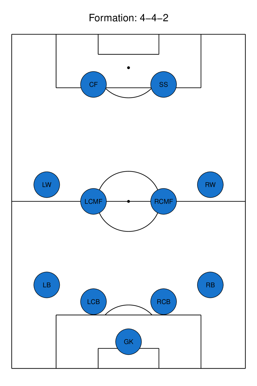
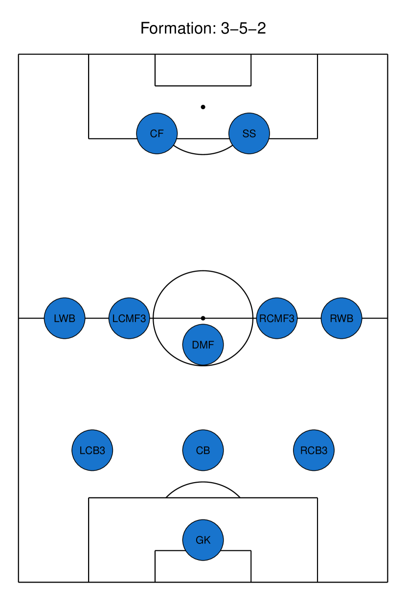
Figure 1: Two popular formations of soccer teams, known as 4-4-2 and 3-5-2. The abbreviations of player positions are detailed in Supplement B.

• Soccer teams consist of more players and the interactions among the players are more complex than, e.g., in basketball and other team-based sports. The fact that soccer teams are larger than teams in many other team-based sports implies that the actions of players on the field need to be coordinated. To facilitate coordination, each soccer team adopts a formation, which assigns each player in the team to a specific position (e.g., goalkeeper, striker). Two popular formations of soccer teams, known as 4-4-2 and 3-5-2, are shown in Figure 1 in Supplement A. The chosen formation can affect the defensive and offensive strategies of a soccer team and can hence affect the outcome of a match. In addition, players may have different roles in different formations, and the formations of teams may change during matches.

• Soccer matches are zero-sum games: One team’s gain is another team’s loss. For example, if the ball changes hands, one team loses control of the ball while the other team gains control of the ball.

We address the lack of a comprehensive statistical analysis of the network of interactions among soccer players by introducing a continuous-time stochastic process, which helps shed light on

• which player controls the ball and how long, and how ball control depends on the player’s attributes (including the player’s position in the team’s formation and the player’s spatial position on the field, provided that the spatial positions of players on the field are known);

• whether a change in ball control is a failure (i.e., the ball is lost to the opposing team) or a success (i.e., the ball remains within the team in control of the ball), and how the probability of a failure or a success depends on attributes of players;

• whether a team on track to winning a match decreases its pace and plays more defensively, while its opponent increases its pace and plays more offensively to change the outcome of the match in its favor;

• unobserved attributes of players that may affect ball control and interactions among players.

1.1 Comparison with non-network models of sport data

In contrast to the literature on basketball and other team-based sports, we do not focus on individual summaries, such as the expected ball possession of individual players (e.g., Cervone et al., 2016; Santos-Fernandez et al., 2022). Instead, we focus on the network of interactions among players, because the performance of a team is more than the sum of the strengths of its players. In other words, a collection of strong players may or may not form a strong soccer team: Whether a collection of players forms a strong soccer team depends on the one hand on the strength of the individual players and on the other hand on how the players interact.

Some recent publications (e.g., chacoma2020modeling; hirotsu2023soccer; narizuka2023validation) have studied soccer matches by using probabilistic models, but the mentioned publications focus on time-dependent motion processes and ignore the network of interactions among players. By contrast, the proposed stochastic modeling framework focuses on the network of interactions among players and helps incorporate the formations of soccer teams in addition to the spatial distances between players, provided that the spatial positions of players are known.

Compared with the continuous-time within-play valuation models of American football in yurko2020going, the proposed stochastic modeling framework focuses on the pace of soccer matches, who is in control of the ball, whether a change in ball control is a failure or a success, and who secures control of the ball, rather than focusing on action evaluations. As a result, the proposed stochastic modeling framework can provide a more comprehensive understanding of team work in soccer and other team-based sports than the existing literature.

1.2 Comparison with discrete-time models of sport data

State-space models and other discrete-time stochastic processes have been used as predictive models for National Football League (NFL) game scores and other team-based sports (e.g., glickman2005state; shaw2019dynamic). By contrast, we focus on continuous-time Markov processes, for at least two reasons.

First, continuous-time Markov processes are natural models of real-world processes where events can occur at any time $t\in[0,+\infty)$, including fast-paced soccer matches.

Second, continuous-time Markov processes can be viewed as discrete-time Markov chains with the time gaps between transitions of the Markov chains filled with Exponential holding times (see, e.g., Chapter 3 of Norris, 1997). In other words, continuous-time Markov processes model when changes take place, and which changes take place. Therefore, continuous-time Markov processes help build richer models than discrete-time Markov processes. For example, in applications to soccer matches, continuous-time Markov processes help shed light on:

• Clock: When a change in ball control occurs, and how a change depends on the attributes of the player in control of the ball.

• Transitions: Who passes the ball to whom, and how a change in ball control depends on the attributes of the players involved.

1.3 Comparison with relational event models

The closest relatives of the proposed stochastic modeling framework may be relational event models (e.g., Butts, 2008; Perry and Wolfe, 2013). That said, there are important differences between relational event models and the proposed stochastic modeling framework:

• Soccer matches revolve around the ball. A reasonable stochastic model of soccer matches needs to reflect the fact that soccer matches revolve around the ball: e.g., at any given time $t$, a single player is in control of the ball and can initiate a relational event (e.g., a pass), and a stochastic model of soccer matches should reflect that. By contrast, relational event models assume that any actor can initiate a relational event at any time: e.g., at any given time $t$, any employee of a company can send an email to one or more other employees.

• Soccer matches are zero-sum games: One team’s gain is another team’s loss. As a result, a reasonable stochastic model of soccer matches should distinguish between successful and unsuccessful relational events (e.g., passes), which can affect the outcomes of a match. By contrast, relational event models are not concerned with zero-sum games and do not distinguish between successful and unsuccessful relational events: e.g., email communications between the employees of a company are not zero-sum games, and the event that employee A sends an email to employee B does not necessarily result in a gain or a loss for employee A or employee B.

• The formations of soccer teams and the locations of players on the field can affect the outcome of a match. By contrast, if an employee of a company considers sending an email, the location of the employee is unimportant: As long as the employee is connected to the World Wide Web, the employee can send an email from any location on planet Earth.

1.4 Structure of paper

We first introduce the data that motivated the proposed stochastic modeling framework (Section 2) and then introduce the stochastic modeling framework (Section 3). A Bayesian approach to learning the stochastic modeling framework from data is described in Section 4, and Bayesian computing is discussed in Section 5. An application to the motivating data is presented in Section 6. Simulation results can be found in Section 7.

2 High-resolution network data

We consider data provided by Hudl & Wyscout (https://footballdata.wyscout.com/). The data consists of 380 matches during the 2020/21 season of Serie A, the premier league of the Italian football league system. The data include ball-tracking data, but not player-tracking data. In other words, we know which player is in control of the ball, but we do not know where the players are located on the field.

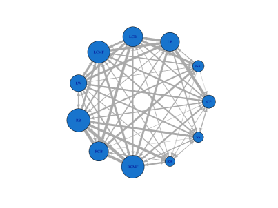
(a) Juventus Turin (4-4-2)

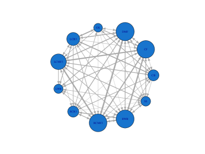
(b) Inter Milan (3-5-2)

Figure 2: The numbers of passes between the positions of (a) Juventus Turin (with 4-4-2 formation) and (b) Inter Milan (with 3-5-2 formation). These data are based on the home games of (a) Juventus Turin versus AC Milan and (b) Inter Milan versus AC Milan in 2020/21. The 4-4-2 and 3-5-2 formations are shown in Figure 1 in Supplement A. The sizes of the positions are proportional to the number of passes, while the widths of the edges are proportional to the number of passes between the positions.

Figure 2 in Supplement A shows a subset of the data: passes between the players of Juventus Turin (with 4-4-2 formation) and Inter Milan (with 3-5-2 formation). These data are based on the home games of Juventus Turin versus AC Milan and Inter Milan versus AC Milan in 2020/21. The figure reveals that passes depend on the formations of teams. Figure 2(a) in Supplement A shows that the midfield players and defenders of Juventus Turin (with 4-4-2 formation) dominate ball control. By contrast, strikers do not control the ball all too often, but are key to scoring goals and hence winning matches. Figure 2(b) in Supplement A reveals that the midfield players of Inter Milan (with 3-5-2 formation) likewise dominate ball control. In addition, the right wing of Inter Milan plays an important role in Inter Milan’s 3-5-2 formation, by passing the ball to the strikers and in so doing helping the team launch counterattacks straight out of the backfield. Other descriptive summaries, including detailed information on the formations and players of Juventus Turin, Inter Milan, and other soccer clubs in Serie A are presented in Supplement C.

3 Stochastic modeling framework

We introduce a continuous-time stochastic process as a model of soccer matches starting at time $t_{0}\coloneqq 0$ and stopping at time $T\in[90,+\infty)$.

Soccer matches involve two competing teams. Each team consists of $11$ players and can substitute up to $5$ players during a match, effective 2022/23. Let $\mathscr{T}_{1,t}$ be the set of players of one of the two teams and $\mathscr{T}_{t,2}$ be the set of players of the opposing team at time $t\in[0,\,T)$. The two sets $\mathscr{T}_{1,t}$ and $\mathscr{T}_{2,t}$ are disjoint, in the sense that $\mathscr{T}_{1,t}\,\cap\,\mathscr{T}_{2,t}=\{\}$ for all $t\in[0,\,T)$. The compositions of the two teams $\mathscr{T}_{1,t}$ and $\mathscr{T}_{2,t}$ can change during a match, because players may be injured; players may be substituted; and the referee may remove players from the field due to violations of rules. We consider changes in the compositions of $\mathscr{T}_{1,t}$ and $\mathscr{T}_{2,t}$ to be exogenous.

3.1 Generic continuous-time stochastic process

We introduce a generic continuous-time stochastic process that captures salient features of soccer matches.

Scoring goals: rare events. We focus on who is control of the ball, whether a change in ball control is a failure or a success, and who secures control of the ball, but we do not model the process of scoring goals. While scoring goals is important for winning matches, the event of scoring a goal is a rare event and useful predictors are hard to come by, because scoring a goal requires a sequence of complex interactions among players of two competing teams. We leave the construction of models for scoring goals to future research and focus here on ball control and interactions among players, which are important for scoring goals and winning matches.

Ball control and interactions among players. We first describe a generic continuous-time stochastic process. We then introduce a specification of the continuous-time stochastic process in Section 3.2 and discuss basic properties of the continuous-time stochastic process in Section 3.3.

A generic continuous-time stochastic process of a soccer match starting at time $t_{0}\coloneqq 0$ and stopping at time $T\in[90,+\infty)$ takes the following form:

1. At time $t_{0}\coloneqq 0$, the referee starts the match. The player who secures control of the ball at time $t_{0}$ is chosen at random from the set $\mathscr{T}_{1,t_{0}}\,\cup\;\mathscr{T}_{2,t_{0}}$ and is denoted by $i_{1}$.

2. At time $t_{m}\coloneqq t_{m-1}+h_{m}$ ($m=1,2,\dots$), the ball passes from player $i_{m}\in\mathscr{T}_{1,t_{m}}\,\cup\;\mathscr{T}_{2,t_{m}}$ to player $j_{m}\in\mathscr{T}_{1,t_{m}}\,\cup\;\mathscr{T}_{2,t_{m}}\setminus\,\{i_{m}\}$, where $h_{m}\sim\mbox{Exponential}(\lambda_{i_{m}})$ and $i_{m}=j_{m-1}$ ($m=2,3,\dots$). The process of passing the ball from player $i_{m}$ to player $j_{m}$ is decomposed as follows:

   1. The change in ball control is either a failure (indicated by $S_{i_{m}}=0$) in that player $i_{m}$ loses the ball to a player of the opposing team, or is a success (indicated by $S_{i_{m}}=1$) in that $i_{m}$ succeeds in passing the ball to a player of $i_{m}$’s own team.

   2. Conditional on $S_{i_{m}}\in\{0,1\}$, player $i_{m}$ cedes control of the ball to player $j_{m}\in\mathscr{T}_{1,t_{m}}\cup\mathscr{T}_{2,t_{m}}\setminus\,\{i_{m}\}$, indicated by $i_{m}\to j_{m}$.

3. The referee stops the match at time $T\in[90,+\infty)$.

We consider the decision of the referee to stop the match to be exogenous, so that the stopping time $T\in[90,+\infty)$ of the match is non-random. In practice, soccer matches last 90 minutes, but disruptions of matches due to injuries and substitutions of players may result in overtime.

3.2 Specification of continuous-time stochastic process

We introduce a specification of the generic continuous-time stochastic process introduced in Section 3.1, by specifying the distributions of the holding times $h_{m}$, the success probabilities $\mathbb{P}(S_{i_{m}}=s_{i_{m}})$, and the pass probabilities $\mathbb{P}(i_{m}\to j_{m}\mid S_{i_{m}}=s_{i_{m}})$. Basic properties of the resulting continuous-time stochastic process are discussed in Section 3.3. Throughout, we denote by $\mathcal{I}_{m}$ the team of player $i_{m}$ in control of the ball at time $t_{m}$.

Holding time distributions

A natural specification of the holding time distributions is

$$\begin{array}[]{lllllllllllll}h_{m}\mid\lambda_{i_{m}}&\mathop{\rm\sim}\limits^{\mbox{\tiny ind}}&\mbox{Exponential}(\lambda_{i_{m}}).\end{array}$$

To allow the rate $\lambda_{i_{m}}\in(0,+\infty)$ of player $i_{m}$’s holding time $h_{m}$ to depend on observed attributes of $i_{m}$ (e.g., the position of $i_{m}$ in the formation of $i_{m}$’s team and the location of $i_{m}$ on the field), we assume that

$$\begin{array}[]{lllllllllllll}\lambda_{i_{m}}(\bm{\omega})&\coloneqq&\exp(\bm{\omega}^{\top}\bm{c}_{i_{m}}),\end{array}$$

where $\bm{\omega}\in\mathbb{R}^{p}$ is a vector of $p$ parameters and $\bm{c}_{i_{m}}\in\mathbb{R}^{p}$ is a vector of $p$ observed attributes of player $i_{m}$.

Success probabilities

The probability of a successful pass $\{S_{i_{m}}=1\}$ by player $i_{m}$ can be specified by a logit model:

$$\begin{array}[]{lllllllllllll}\mbox{logit}(\mathbb{P}_{\bm{\alpha},\bm{\eta}}(S_{i_{m}}=1))&\coloneqq&\bm{\alpha}^{\top}\bm{x}_{1,i_{m}}+\eta_{1,i_{m}},\end{array}$$

where $\bm{\alpha}\in\mathbb{R}^{d_{1}}$ is a vector of $d_{1}$ parameters and $\bm{x}_{1,i_{m}}\in\mathbb{R}^{d_{1}}$ is a vector of $d_{1}$ observed attributes of player $i_{m}$. The random effect $\eta_{1,i_{m}}\in\mathbb{R}$ captures the effect of unobserved attributes of player $i_{m}$ on the success probability.

Pass probabilities

The conditional probability of event $\{i_{m}\to j_{m}\}$ given $\{S_{i_{m}}=0\}$ can be specified by a multinomial logit model:

$$\begin{array}[]{lllllllllllll}\mathbb{P}_{\bm{\beta},\bm{\eta}}(i_{m}\to j_{m}\mid S_{i_{m}}=0)\vspace{0.25cm}\\ \coloneqq\;\left\{\begin{array}[]{lll}\dfrac{\exp(\bm{\beta}^{\top}\bm{x}_{2,i_{m},j_{m}}+\eta_{2,j_{m}})}{\sum_{j\,\not\in\,\mathcal{I}_{m}}\exp(\bm{\beta}^{\top}\bm{x}_{2,i_{m},j}+\eta_{2,j})}&\mbox{if }j_{m}\not\in\mathcal{I}_{m}\\ 0&\mbox{if }j_{m}\in\mathcal{I}_{m},\end{array}\right\}\end{array}$$

where $\bm{\beta}\in\mathbb{R}^{d_{2}}$ is a vector of $d_{2}$ parameters and $\bm{x}_{2,i_{m},j}\in\mathbb{R}^{d_{2}}$ is a vector of $d_{2}$ observed attributes of players $i_{m}$ and $j$. The random effect $\eta_{2,j}\in\mathbb{R}$ captures the effect of unobserved attributes of player $j$ on the conditional probability of securing control of the ball.

Along the same lines, the conditional probability of event $\{i_{m}\to j_{m}\}$ given $\{S_{i_{m}}=1\}$ can be specified by a multinomial logit model:

$$\begin{array}[]{lllllllllllll}\mathbb{P}_{\bm{\gamma},\bm{\eta}}(i_{m}\to j_{m}\mid S_{i_{m}}=1)\vspace{0.25cm}\\ \coloneqq\;\left\{\begin{array}[]{lll}0&\mbox{if }i_{m}=j_{m}\mbox{ or }j_{m}\not\in\mathcal{I}_{m}\\ \dfrac{\exp(\bm{\gamma}^{\top}\bm{x}_{3,i_{m},j_{m}}+\eta_{3,j_{m}})}{\sum_{j\,\in\,\mathcal{I}_{m}\setminus\{i_{m}\}}\exp(\bm{\gamma}^{\top}\bm{x}_{3,i_{m},j}+\eta_{3,j})}&\mbox{if }i_{m}\neq j_{m}\mbox{ and }j_{m}\in\mathcal{I}_{m},\end{array}\right.\end{array}$$

where $\bm{\gamma}\in\mathbb{R}^{d_{3}}$ is a vector of $d_{3}$ parameters and $\bm{x}_{3,i_{m},j}\in\mathbb{R}^{d_{3}}$ is a vector of $d_{3}$ observed attributes of players $i_{m}$ and $j$, e.g., whether player $i_{m}$ passed the ball to player $j$ in the past, whether player $i_{m}$ received the ball from player $j$ in the past, or the spatial distance between players $i_{m}$ and $j$ at the time of the pass (provided that the spatial positions of players are known). The random effect $\eta_{3,j}\in\mathbb{R}$ captures the effect of unobserved attributes of player $j$ on the conditional probability of securing control of the ball.

Random effects

Let $\bm{\eta}_{i}\coloneqq(\eta_{1,i},\,\eta_{2,i},\,\eta_{3,i})\in\mathbb{R}^{3}$ and assume that

$$\begin{array}[]{lllllllllllll}\bm{\eta}_{i}\mid\mbox{\boldmath$\Sigma$}&\mathop{\rm\sim}\limits^{\mbox{\tiny iid}}&\mbox{MVN}_{3}(\bm{0}_{3},\,\mbox{\boldmath$\Sigma$}),\end{array}$$

where $\bm{0}_{3}\in\mathbb{R}^{3}$ is the three-dimensional null vector and $\mbox{\boldmath$\Sigma$}\in\mathbb{R}^{3\times 3}$ is a positive-definite variance-covariance matrix.

Alternative models   It is worth noting that there are other possible approaches to constructing stochastic models of soccer matches. For example, each the two following approaches to constructing models can help shed light on salient aspects of soccer matches:

• Assuming player $i_{m}$ is in control of the ball at time $t_{m}$, first determine whether $i_{m}$ succeeds in passing the ball to a teamplayer. Then determine which teamplayer $j_{m}$ receives the ball provided that the pass is a success, otherwise determine which player $j_{m}$ of the opposing team secures control of the ball provided that the pass is a failure (the approach pursued here).

• Assuming player $i_{m}$ is in control of the ball at time $t_{m}$, suppose that $i_{m}$ first selects a teamplayer $k_{m}$ and intends to pass the ball to $k_{m}$. Then determine whether the intended pass $i_{m}\to k_{m}$ succeeds. If the intended pass $i_{m}\to k_{m}$ succeeds, set $k_{m}=j_{m}$, otherwise select the player $j_{m}$ who secures control of the ball from the opposing team (an approach suggested by an anonymous referee).

While both approaches can be useful, there are two good reasons for choosing approach (a), that is, the approach pursued here.

First, soccer matches revolve around the ball, so soccer teams wish to retain control of the ball. Thus, the player in control of the ball is first and foremost responsible for passing the ball to a teamplayer—unless the player has the rare opportunity to score a goal. By construction, approach (a) respects the importance of retaining control of the ball.

Second, approach (a) has one advantage over approach (b): If a pass is a failure, we do not observe the intended receiver $k_{m}$. Worse, even when a pass is a success, we may not observe the intended receiver $k_{m}$: e.g., $i_{m}$ may intend to pass the ball to teamplayer $k_{m}$, but the ball ends up in possession of some other teamplayer $j_{m}\neq k_{m}$ by accident. In fact, instead of observing the intended receiver $k_{m}$, we observe the actual receiver $j_{m}$, who may or may not be identical to the intended receiver $k_{m}$. In other words, the data fall short, in that we do not observe the intended passes $i_{m}\to k_{m}$, but we observe the actual passes $i_{m}\to j_{m}$, regardless of whether the passes are failures or successes. As a result, approach (b) would require augmenting the observed passes $i_{m}\to j_{m}$ by the unobserved, intended passes $i_{m}\to k_{m}$. While it is possible to augment the observed passes $i_{m}\to j_{m}$ by the unobserved, intended passes $i_{m}\to k_{m}$ using data-augmentation methods, such methods come at additional computational costs compared with approach (a). In addition, there may be statistical costs: It is not clear how much information the data contain about the unobserved, intended passes $i_{m}\to k_{m}$.

3.3 Properties of continuous-time stochastic process

We discuss basic properties of the continuous-time stochastic process specified in Sections 3.1 and 3.2. Throughout Section 3.3, we suppress the notational dependence of all quantities on the parameters $\bm{\alpha},\,\bm{\beta},\,\bm{\gamma},\,\bm{\omega},\,\bm{\Sigma}$ and the random effects $\bm{\eta}_{1},\bm{\eta}_{2},\dots$We assume that the continuous-time stochastic process satisfies two assumptions:

• In a short time interval $[t_{1},\,t_{2}]$, the compositions of teams $\mathscr{T}_{1,t}$ and $\mathscr{T}_{2,t}$ are constant, in the sense that $\mathscr{T}_{1,t}\equiv\mathscr{T}_{1}$ and $\mathscr{T}_{2,t}\equiv\mathscr{T}_{2}$ for all $t\in[t_{1},\,t_{2})$, and the 22 players of the two teams are labeled $1,\dots,22$.

• In a short time interval $[t_{1},\,t_{2}]$, the attributes of players and teams, the rates $\lambda_{i}$, the success probabilities $\mathbb{P}(S_{i}=s_{i})$, and the pass probabilities $\mathbb{P}(i\to j\mid S_{i}=s_{i})$ are time-invariant.

Assumption A.1 states that the compositions of the teams do not change in a short time interval, that is, the two teams do not substitute players. Assumption A.2 ensures that the continuous-time stochastic process is time-homogeneous in a short time interval. The assumption that the continuous-time stochastic process is time-homogeneous in a short time interval is not unreasonable, because soccer teams consist of humans, and humans are incapable of instantaneous changes. We hasten to point out that the stochastic modeling framework is not restricted to time-homogeneous stochastic processes: It does allow the attributes of players and teams, the rates $\lambda_{i}$, the success probabilities $\mathbb{P}(S_{i}=s_{i})$, and the pass probabilities $\mathbb{P}(i\to j\mid S_{i}=s_{i})$ to change over time. The purpose of the following proposition is to shed light on the behavior of the continuous-time stochastic process in a short time interval, during which the stochastic process can be approximated by a time-homogeneous stochastic process.

Proposition 1. Consider the continuous-time stochastic process described in Sections 3.1 and 3.2 satisfying Assumptions A.1 and A.2. Then the stochastic process is a right-continuous and time-homogeneous Markov process $\{Y(t),\,t\in[t_{1},\,t_{2})\}$ with finite state space $\mathscr{Y}\coloneqq\{1,\dots,22\}$ during a short time interval $[t_{1},t_{2})$, where the state $Y(t)\in\mathscr{Y}$ of the Markov process at time $t$ indicates which player is in control of the ball at time $t$. The elements $q_{i,j}$ of the generator matrix $\bm{Q}\in\mathbb{R}^{|\mathscr{Y}|\times|\mathscr{Y}|}$ of the Markov process are

$$\begin{array}[]{lllllllllllll}q_{i,j}&\coloneqq&\left\{\begin{array}[]{lll}\lambda_{i}\;\,\mathbb{P}(S_{i}=0)\;\,\mathbb{P}(i\to j\mid S_{i}=0)&\mbox{if }i\neq j\mbox{ and }j\not\in\mathcal{I}_{i}\\ \lambda_{i}\;\,\mathbb{P}(S_{i}=1)\;\,\mathbb{P}(i\to j\mid S_{i}=1)&\mbox{if }i\neq j\mbox{ and }j\in\mathcal{I}_{i}\\ -\lambda_{i}&\mbox{if }i=j,\end{array}\right\}\end{array}$$

where $\mathcal{I}_{i}$ denotes the team of player $i\in\mathscr{Y}$. Consider any $t\in[t_{1},\,t_{2})$ and any $h\in(0,\,t_{2}-t)$. Then, for all $(i,j)\in\mathscr{Y}^{2}$, conditional on $\{Y(t)=i\}$, the event $\{Y(t+h)=j\}$ is independent of $\{Y(s),\,s\leq t\}$ and, as $h\downarrow 0$, the conditional probability of event $\{Y(t+h)=j\}$ given $\{Y(t)=i\}$ is

$$\begin{array}[]{lllllllllllll}\mathbb{P}(Y(t+h)=j\mid Y(t)=i)&=&\delta_{i,j}+q_{i,j}\,h+o(h),\end{array}$$

where $\delta_{i,j}\coloneqq 1$ if $i=j$ and $\delta_{i,j}\coloneqq 0$ otherwise.

The proposition is a straightforward consequence of the construction of the continuous-time stochastic process and Theorem 2.8.2 of  Norris (1997, p. 94). The proposition shows that the continuous-time stochastic process focuses on ball control and who passes the ball to whom, by specifying the rates $q_{i,j}$ of passing the ball between pairs of players $(i,j)\in\mathcal{Y}^{2}$. It implies that the conditional probability of the event that player $j$ is in possession of the ball at time $t+h$, given that player $i\neq j$ is in possession of the ball at time $t$, is approximately $q_{i,j}\,h$ in a short time interval of length $h$.

4 Bayesian learning

We pursue a Bayesian approach to learning the stochastic modeling framework introduced in Section 3 from high-resolution network data.

A Bayesian approach is well-suited to online learning, that is, updating the knowledge about the parameters $\bm{\alpha},\,\bm{\beta},\,\bm{\gamma},\,\bm{\omega},\,\bm{\Sigma}$ and the random effects $\bm{\eta}_{1},\bm{\eta}_{2},\dots$ as soon as additional data points roll in. To demonstrate, consider two teams and let $\bm{x}_{1}\coloneqq(h_{1,m},\,i_{1,m},\,j_{1,m})_{m=1}^{M_{1}}$ be the outcome of the first match of the two teams (with $M_{1}\geq 1$ passes) and $\bm{x}_{2}\coloneqq(h_{2,m},\,i_{2,m},\,j_{2,m})_{m=1}^{M_{2}}$ be the outcome of the second match of the two teams (with $M_{2}\geq 1$ passes). To ease the presentation, assume that the compositions of the two teams do not change during the first and second match, the 22 players of the two teams are labeled $1,\dots,22$, and the random effects are denoted by $\bm{\eta}\coloneqq(\bm{\eta}_{1},\dots,\bm{\eta}_{22})$. In addition, assume that the outcomes of the first and second match $\bm{x}_{1}$ and $\bm{x}_{2}$ satisfy

$$\begin{array}[]{lllllllllllll}\pi(\bm{x}_{1},\,\bm{x}_{2}\mid\bm{\alpha},\,\bm{\beta},\,\bm{\gamma},\,\bm{\omega},\,\bm{\eta})&=&\pi(\bm{x}_{1}\mid\bm{\alpha},\,\bm{\beta},\,\bm{\gamma},\,\bm{\omega},\,\bm{\eta})\\ &\times&\pi(\bm{x}_{2}\mid\bm{\alpha},\,\bm{\beta},\,\bm{\gamma},\,\bm{\omega},\,\bm{\eta},\,\bm{x}_{1}),\end{array}$$

where $\pi$ denotes a generic probability density function. The conditional probability density function $\pi(\bm{x}_{1}\mid\bm{\alpha},\,\bm{\beta},\,\bm{\gamma},\,\bm{\omega},\,\bm{\eta})$ is of the form

$$\begin{array}[]{lllllllllllll}\pi(\bm{x}_{1}\mid\bm{\alpha},\,\bm{\beta},\,\bm{\gamma},\,\bm{\omega},\,\bm{\eta})\;=\;\displaystyle\prod\limits_{m=1}^{M_{1}}\,\Big{[}\lambda_{i_{1,m}}(\bm{\omega})\,\exp(-\lambda_{i_{1,m}}(\bm{\omega})\,h_{1,m})\vspace{0.25cm}\\ \hskip 135.15059pt\times\;\;\mathbb{P}_{\bm{\alpha},\bm{\eta}}(S_{i_{1,m}}=s_{i_{1,m}})\vspace{0.25cm}\\ \hskip 135.15059pt\times\;\;\mathbb{P}_{\bm{\beta},\bm{\eta}}(i_{1,m}\to j_{1,m}\mid S_{i_{1,m}}=0)^{\mathbbm{1}(S_{i_{1,m}}=\;0)}\vspace{0.25cm}\\ \hskip 135.15059pt\times\;\;\mathbb{P}_{\bm{\gamma},\bm{\eta}}(i_{1,m}\to j_{1,m}\mid S_{i_{1,m}}=1)^{\mathbbm{1}(S_{i_{1,m}}=\;1)}\Big{]}\vspace{0.25cm}\vspace{0.25cm}\\ \hskip 135.15059pt\times\;\;\exp\left(-\lambda_{i_{1,M_{1}+1}}(\bm{\omega})\,\left(T_{1}-\displaystyle\sum\limits_{k=1}^{M_{1}}h_{1,k}\right)\right),\end{array}$$

assuming that the start time $t_{0}\coloneqq 0$ and the stopping time $T_{1}\in[90,+\infty)$ of the match are determined by the referee and are both non-random. The function $\mathbbm{1}(.)$ is an indicator function, which is $1$ if its argument is true and is $0$ otherwise. The conditional probability density function $\pi(\bm{x}_{2}\mid\bm{\alpha},\,\bm{\beta},\,\bm{\gamma},\,\bm{\omega},\,\bm{\eta},\,\bm{x}_{1})$ is of the same form as $\pi(\bm{x}_{1}\mid\bm{\alpha},\,\bm{\beta},\,\bm{\gamma},\,\bm{\omega},\,\bm{\eta})$, but is based on $M_{2}$ passes rather than $M_{1}$ passes and can depend on the outcome of the first match $\bm{x}_{1}$.

The posterior of $\bm{\alpha},\,\bm{\beta},\,\bm{\gamma},\,\bm{\omega},\,\bm{\Sigma},\,\bm{\eta}$ based on the outcome of the first match $\bm{x}_{1}$ is proportional to

$$\begin{array}[]{llllllllll}\pi(\bm{\alpha},\,\bm{\beta},\,\bm{\gamma},\,\bm{\omega},\,\bm{\Sigma},\,\bm{\eta}\mid\bm{x}_{1})&\propto&\pi(\bm{x}_{1}\mid\bm{\alpha},\,\bm{\beta},\,\bm{\gamma},\,\bm{\omega},\,\bm{\eta})\\ &\times&\pi(\bm{\eta}\mid\bm{\Sigma})\;\pi(\bm{\alpha},\,\bm{\beta},\,\bm{\gamma},\,\bm{\omega},\,\bm{\Sigma}),\end{array}$$

where $\pi(\bm{\alpha},\,\bm{\beta},\,\bm{\gamma},\,\bm{\omega},\,\bm{\Sigma})$ is the prior of $\bm{\alpha},\,\bm{\beta},\,\bm{\gamma},\,\bm{\omega},\,\bm{\Sigma}$. The prior of $\bm{\alpha},\,\bm{\beta},\,\bm{\gamma},\,\bm{\omega},\,\bm{\Sigma}$ is described in Section 5.

As soon as the outcome of the second match $\bm{x}_{2}$ is observed, the knowledge about $\bm{\alpha},\,\bm{\beta},\,\bm{\gamma},\,\bm{\omega},\,\bm{\Sigma},\,\bm{\eta}$ in light of $\bm{x}_{2}$ can be updated as follows:

$$\begin{array}[]{lllllllllllll}\begin{array}[]{llllllllll}&&\pi(\bm{\alpha},\,\bm{\beta},\,\bm{\gamma},\,\bm{\omega},\,\bm{\Sigma},\,\bm{\eta}\mid\bm{x}_{1},\,\bm{x}_{2})\\ &\propto&\pi(\bm{x}_{1},\,\bm{x}_{2}\mid\bm{\alpha},\,\bm{\beta},\,\bm{\gamma},\,\bm{\omega},\,\bm{\eta})\;\pi(\bm{\eta}\mid\bm{\Sigma})\;\pi(\bm{\alpha},\,\bm{\beta},\,\bm{\gamma},\,\bm{\omega},\,\bm{\Sigma})\\ &\propto&\pi(\bm{x}_{2}\mid\bm{\alpha},\,\bm{\beta},\,\bm{\gamma},\,\bm{\omega},\,\bm{\eta},\,\bm{x}_{1})\;{\pi(\bm{\alpha},\,\bm{\beta},\,\bm{\gamma},\,\bm{\omega},\,\bm{\Sigma},\,\bm{\eta}\mid\bm{x}_{1})}.\end{array}\end{array}$$

In other words, as soon as the outcome of the second match $\bm{x}_{2}$ is observed, we can update the knowledge about $\bm{\alpha},\,\bm{\beta},\,\bm{\gamma},\,\bm{\omega},\,\bm{\Sigma},\,\bm{\eta}$ in light of $\bm{x}_{2}$ via $\pi(\bm{x}_{2}\mid\bm{\alpha},\,\bm{\beta},\,\bm{\gamma},\,\bm{\omega},\,\bm{\eta},\,\bm{x}_{1})$, with the knowledge about $\bm{\alpha},\,\bm{\beta},\,\bm{\gamma},\,\bm{\omega},\,\bm{\Sigma},\,\bm{\eta}$ prior to the second match $\bm{x}_{2}$ being quantified by $\pi(\bm{\alpha},\,\bm{\beta},\,\bm{\gamma},\,\bm{\omega},\,\bm{\Sigma},\,\bm{\eta}\mid\bm{x}_{1})$, the posterior based on the outcome of the first match $\bm{x}_{1}$. As a result, a Bayesian approach is a natural approach to updating knowledge about the stochastic modeling framework as additional data points roll in. More than two teams with can be handled, and multiple matches in parallel.

5 Bayesian computing

The posterior $\pi(\bm{\alpha},\,\bm{\beta},\,\bm{\gamma},\,\bm{\omega},\,\bm{\Sigma},\,\bm{\eta}\mid\bm{x})$ of the parameters $\bm{\alpha},\,\bm{\beta},\,\bm{\gamma},\,\bm{\omega},\,\bm{\Sigma}$ and the random effects $\bm{\eta}$ based on the outcome of a match $\bm{x}$ is not available in closed form. We approximate the posterior by using Markov chain Monte Carlo methods, by sampling from the full conditional distributions of the parameters and the random effects:

$$\begin{array}[]{lllllllllllll}\pi(\bm{\alpha}\mid\bm{x})&\propto&\mathscr{L}(\bm{\alpha},\bm{\eta};\,\bm{x})\,\pi(\bm{\alpha})\vspace{0.25cm}\\ \pi(\bm{\beta}\mid\bm{x})&\propto&\mathscr{L}(\bm{\beta},\bm{\eta};\,\bm{x})\,\pi(\bm{\beta})\vspace{0.25cm}\\ \pi(\bm{\gamma}\mid\bm{x})&\propto&\mathscr{L}(\bm{\gamma},\bm{\eta};\,\bm{x})\,\pi(\bm{\gamma})\vspace{0.25cm}\\ \pi(\bm{\omega}\mid\bm{x})&\propto&\mathscr{L}(\bm{\omega};\,\bm{x})\,\pi(\bm{\omega})\vspace{0.25cm}\\ \pi(\bm{\eta}\mid\bm{x})&\propto&\mathscr{L}(\bm{\alpha},\bm{\eta};\,\bm{x})\,\mathscr{L}(\bm{\beta},\bm{\eta};\,\bm{x})\,\mathscr{L}(\bm{\gamma},\bm{\eta};\,\bm{x})\,\mathscr{L}(\mbox{\boldmath$\Sigma$};\,\bm{\eta})\vspace{0.25cm}\\ \pi(\bm{\Sigma}\mid\bm{\eta})&\propto&\mathscr{L}(\mbox{\boldmath$\Sigma$};\,\bm{\eta})\,\pi(\bm{\Sigma}),\end{array}$$

where

$$\begin{array}[]{lllllllllllll}\mathscr{L}(\bm{\alpha},\bm{\eta};\,\bm{x})&\propto&\displaystyle\prod\limits_{m=1}^{M}\,\mathbb{P}_{\bm{\alpha},\bm{\eta}}(S_{i_{m}}=s_{i_{m}})\vspace{0.25cm}\\ \mathscr{L}(\bm{\beta},\bm{\eta};\,\bm{x})&\propto&\displaystyle\prod\limits_{m=1}^{M}\,\mathbb{P}_{\bm{\beta},\bm{\eta}}(i_{m}\to j_{m}\mid S_{i_{m}}=0)^{\mathbbm{1}(S_{i_{m}}=\;0)}\vspace{0.25cm}\\ \mathscr{L}(\bm{\gamma},\bm{\eta};\,\bm{x})&\propto&\displaystyle\prod\limits_{m=1}^{M}\,\mathbb{P}_{\bm{\gamma},\bm{\eta}}(i_{m}\to j_{m}\mid S_{i_{m}}=1)^{\mathbbm{1}(S_{i_{m}}=\;1)}\vspace{0.25cm}\\ \mathscr{L}(\bm{\omega};\,\bm{x})&\propto&\displaystyle\prod\limits_{m=1}^{M}\,\left[\lambda_{i_{m}}(\bm{\omega})\,\exp(-\lambda_{i_{m}}(\bm{\omega})\,h_{m})\right]\,\exp\left(-\lambda_{i_{M+1}}(\bm{\omega})\,\left(T-\displaystyle\sum\limits_{k=1}^{M}h_{k}\right)\right)\vspace{0.25cm}\\ \mathscr{L}(\mbox{\boldmath$\Sigma$};\,\bm{\eta})&\propto&\displaystyle\prod\limits_{i=1}^{n}\,\mbox{det}({\bm{\Sigma}^{-1}})^{1/2}\,\exp\left(-\dfrac{1}{2}\,\bm{\eta}_{i}^{\top}\,\bm{\Sigma}^{-1}\,\bm{\eta}_{i}\right),\end{array}$$

assuming that $\bm{x}$ is the outcome of a single soccer match with $M\geq 1$ passes starting at time $t_{0}=0$ and stopping at time $T\in[90,+\infty)$; note that both the start time $t_{0}$ and the stopping time $T$ are non-random. We assume that the prior factorizes according to

$$\begin{array}[]{lllllllllllll}\pi(\bm{\alpha},\,\bm{\beta},\,\bm{\gamma},\,\bm{\omega},\,\bm{\Sigma})&=&\pi(\bm{\alpha})\,\pi(\bm{\beta})\,\pi(\bm{\gamma})\,\pi(\bm{\omega})\,\pi(\bm{\Sigma}),\end{array}$$

with marginal priors of the form

$$\begin{array}[]{lllllllllllll}\alpha_{k}&\mathop{\rm\sim}\limits^{\mbox{\tiny iid}}&N(0,10^{2}),&k=1,\dots,d_{1},&&\beta_{k}&\mathop{\rm\sim}\limits^{\mbox{\tiny iid}}&N(0,10^{2}),&k=1,\dots,d_{2}\\ \gamma_{k}&\mathop{\rm\sim}\limits^{\mbox{\tiny iid}}&N(0,10^{2}),&k=1,\dots,d_{3},&&\omega_{k}&\mathop{\rm\sim}\limits^{\mbox{\tiny iid}}&N(0,10^{2}),&k=1,\dots,p,\end{array}$$

where $N(0,10^{2})$ is a Gaussian with mean $0$ and variance $10^{2}=100$. To specify the prior of the variance-covariance matrix $\bm{\Sigma}$ of the random effects, we decompose $\bm{\Sigma}$ according to

$$\begin{array}[]{lllllllllllll}\mbox{\boldmath$\Sigma$}&\coloneqq&\left(\begin{array}[]{llll}\sigma_{\eta_{1}}&0&0\\ 0&\sigma_{\eta_{2}}&0\\ 0&0&\sigma_{\eta_{3}}\end{array}\right)\,\bm{\Lambda}\left(\begin{array}[]{llll}\sigma_{\eta_{1}}&0&0\\ 0&\sigma_{\eta_{2}}&0\\ 0&0&\sigma_{\eta_{3}}\end{array}\right),\end{array}$$

where $\bm{\Lambda}\in[-1,+1]^{3\times 3}$ is a correlation matrix. We then assume that $\bm{\Lambda}\sim\mbox{LKJcorr}(2)$ has a Lewandowski-Kurowicka-Joe (LKJ) distribution with parameter $2$ and $\sigma_{\eta_{k}}\mathop{\rm\sim}\limits^{\mbox{\tiny iid}}\mbox{Exponential}(1)$ ($k=1,2,3$).

To sample from the full conditionals, we use Markov chain Monte Carlo methods implemented in R package rstan (Stan Development Team, 2023). Since the stochastic modeling framework leverages exponential-family distributions as building blocks (e.g., Bernoulli, Multinomial, Exponential, and multivariate Gaussians), we do not have more numerical issues than other exponential-family models, such as generalized linear models, Gaussian and non-Gaussian graphical models (efron22).

6 Application

We use the stochastic modeling framework introduced in Section 3 to analyze the data described in Section 2. We focus on the matches of four soccer teams during the 2020/21 season of Serie A, the premier league of the Italian football league system:

• Juventus Turin (Juventus F.C.; 15,832 observations);

• Inter Milan (Internazionale Milano; 13,564 observations);

• Crotone (Crotone S.r.l.; 8,125 observations);

• Fiorentina (ACF Fiorentina; 8,107 observations).

Juventus Turin and Inter Milan belong to the most storied Italian soccer clubs, while Crotone and Fiorentina were mid- and low-level teams during the 2020/21 season, respectively. The numbers of observations mentioned above refer to the total numbers of passes during the 2020/21 season, aggregated over all matches played by the selected teams with the dominant formation. The selected teams have in common that all of them were proficient users of the 4-4-2 formation (Juventus Turin) or the 3-5-2 formation (Inter Milan, Crotone, Fiorentina).

We use the following specification of the stochastic modeling framework:

• Module 1 (M1): The Exponential model of the holding times $h_{m}$ uses the following covariates: position-specific indicators of who is in control of the ball and indicators of whether the player’s team is on track to winning or losing the match (i.e., the player’s team has scored at least one more goal or one less goal than its opponent, respectively).

• Module 2 (M2): The logit model of the probability of a successful pass $\{S_{i_{m}}=1\}$ uses the following covariates, in addition to an intercept: the length of the pass in terms of two-dimensional Euclidean distance; an indicator of whether player $i_{m}$ initiates the pass in the opposing team’s half of the field; an indicator of whether the ball ends up in the opposing team’s third of the field; an indicator of whether the pass is a forward pass; an indicator of whether the pass is an air pass; indicators of whether the player’s team is on track to winning or losing the match (i.e., whether the player’s team has scored at least one more goal or one less goal than its opponent, respectively); and a position-specific random effect.

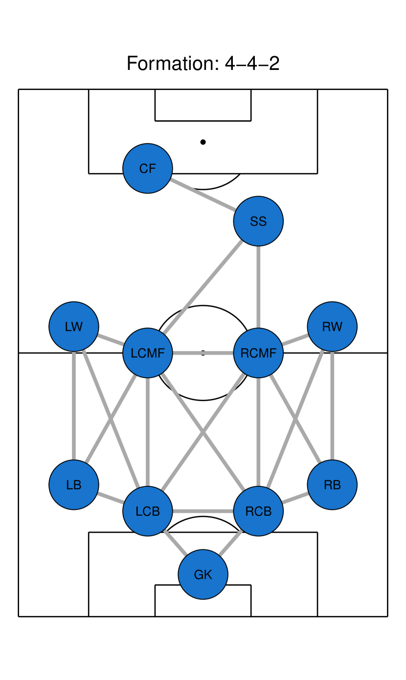
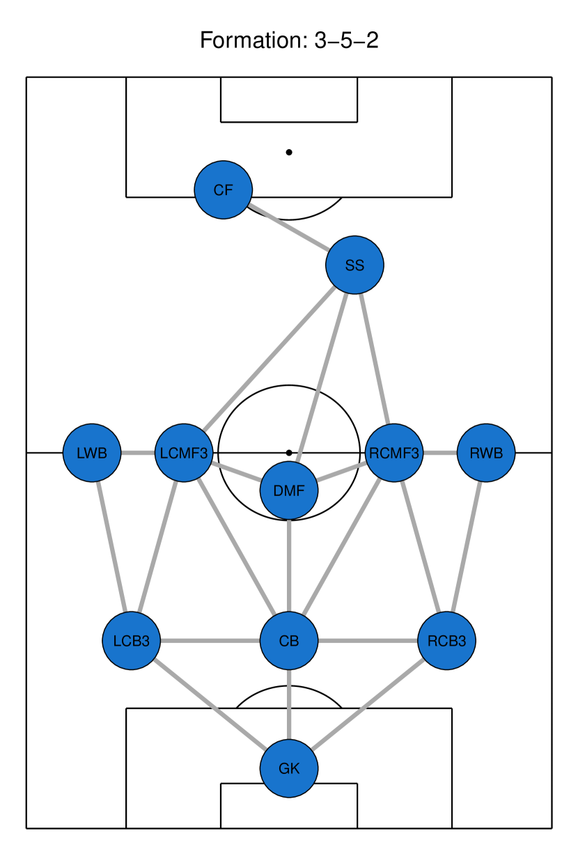
Figure 3: The nearest-neighbor graph, which connects pairs of positions that are considered to be nearest neighbors on the field. The graph distance between a pair of positions is the length of the shortest path between them. The abbreviations of player positions are detailed in Supplement B.

• Module 3 (M3): The multinomial logit model of the conditional probability of event $\{i_{m}\to j_{m}\}$ given $\{S_{i_{m}}=1\}$ uses the following predictors: the graph distance between players $i_{m}$ and $j_{m}$—defined as the length of the shortest path between $i_{m}$ and $j_{m}$—based on the nearest-neighbor graph in Figure 3 in Supplement A; the number of times $j_{m}$ received the ball prior to the $m$-th pass; and a position-specific random effect.

It would be interesting to include more features into the multinomial logit model of the conditional probability of event $\{i_{m}\to j_{m}\}$ given $\{S_{i_{m}}=1\}$, e.g., the spatial positions of players and additional network features. That said, we do not have data on the spatial distances between players and additional network features. Note that these limitations are limitations of the data, not the model: The model can incorporate spatial distances between players as well as additional network features. In addition, note that we focus here on all matches involving the four mentioned teams with the dominant formation, but we do not use the data of the opposing teams. As a consequence, we do not specify the conditional probabilities of events $\{i_{m}\to j_{m}\}$ given $\{S_{i_{m}}=0\}$. Last, but not least, note that we use position-specific rather than player-specific random effects, because the data do not include complete information about which position is filled by which player.

Posterior sensitivity checks and posterior predictive checks can be found in Sections 6.1 and 6.2, respectively: The posterior sensitivity checks suggest that the posterior is not too sensitive to the choice of prior, while the posterior predictive checks indicate that model-based predictions match the observed data. Tables 9 and 10 in Supplement D present posterior summaries of the model parameters, based on the 2020/21 matches of Fiorentina, Crotone, and Inter Milan (with 3-5-2 formation) and Juventus Turin (with 4-4-2 formation). Among other things, these results suggest that all teams reduce the pace of passing the ball when being on track to winning a match. By contrast, when on track to losing a match, Juventus Turin and Inter Milan reduce the pace, whereas Fiorentina and Crotone do not. These results are surprising. As a case in point, consider Inter Milan: When Inter Milan is on track to losing a match, one would expect that Inter Milan either maintains or increases its pace to change the outcome of the match in its favor. But the results suggest otherwise: In the face of defeat, Inter Milan appears to reduce its pace—regardless of whether the opposing team is weak or strong. Juventus Turin appears to do the same. By contrast, Fiorentina and Crotone maintain their pace when on track to losing a match. The difference suggests that the strategies of Juventus Turin and Inter Milan for dealing with adverse situations differ from the strategies of Fiorentina and Crotone. There is an additional observation suggesting that the strategies of Juventus Turin and Inter Milan differ from the strategies of Fiorentina and Crotone: Starting a pass in the opponent’s half of the field does not increase the probability of a successful pass among Fiorentina and Crotone players, but it does increase the probability of a successful pass among Juventus Turin and Inter Milan players. The increase in the probability of a successful pass in the opponent’s half of the field may be due to the offensive strength of Juventus Turin and Inter Milan. Taken together, these results suggest that the strategies of strong teams in the face of defeat differ from those of less strong teams: Strong teams may have the luxury to decrease their pace and leverage their offensive strength, while less strong teams may not be able to do so.

Among the position-specific effects, it is worth noting that the length of time the goal keeper controls the ball tends to be lower than the length of time other positions control the ball. This observation makes sense, because the goal keeper has an incentive to remove the ball from the penalty area as soon as possible, so that the opposing team cannot gain control of the ball in the penalty area and score an easy goal.

6.1 Posterior sensitivity checks

To assess the sensitivity of the posterior to the choice of prior, we consider the following three priors:

• Prior 1:

  $$\begin{array}[]{lllllllllllll}\alpha_{k}&\mathop{\rm\sim}\limits^{\mbox{\tiny iid}}&N(0,5^{2}),&k=1,\dots,d_{1},&&\beta_{k}&\mathop{\rm\sim}\limits^{\mbox{\tiny iid}}&N(0,5^{2}),&k=1,\dots,d_{2}\\ \gamma_{k}&\mathop{\rm\sim}\limits^{\mbox{\tiny iid}}&N(0,5^{2}),&k=1,\dots,d_{3},&&\omega_{k}&\mathop{\rm\sim}\limits^{\mbox{\tiny iid}}&N(0,5^{2}),&k=1,\dots,p;\end{array}$$

• Prior 2, used in Section 6:

  $$\begin{array}[]{lllllllllllll}\alpha_{k}&\mathop{\rm\sim}\limits^{\mbox{\tiny iid}}&N(0,10^{2}),&k=1,\dots,d_{1},&&\beta_{k}&\mathop{\rm\sim}\limits^{\mbox{\tiny iid}}&N(0,10^{2}),&k=1,\dots,d_{2}\\ \gamma_{k}&\mathop{\rm\sim}\limits^{\mbox{\tiny iid}}&N(0,10^{2}),&k=1,\dots,d_{3},&&\omega_{k}&\mathop{\rm\sim}\limits^{\mbox{\tiny iid}}&N(0,10^{2}),&k=1,\dots,p;\end{array}$$

• Prior 3:

  $$\begin{array}[]{lllllllllllll}\alpha_{k}&\mathop{\rm\sim}\limits^{\mbox{\tiny iid}}&N(0,15^{2}),&k=1,\dots,d_{1},&&\beta_{k}&\mathop{\rm\sim}\limits^{\mbox{\tiny iid}}&N(0,15^{2}),&k=1,\dots,d_{2}\\ \gamma_{k}&\mathop{\rm\sim}\limits^{\mbox{\tiny iid}}&N(0,15^{2}),&k=1,\dots,d_{3},&&\omega_{k}&\mathop{\rm\sim}\limits^{\mbox{\tiny iid}}&N(0,15^{2}),&k=1,\dots,p;\end{array}$$

where $N(0,5^{2})$, $N(0,10^{2})$, and $N(0,15^{2})$ are Gaussians with mean $0$ and variances $5^{2}=25$, $10^{2}=100$, and $15^{2}=225$, respectively. The random effects prior is described in Section 5 and is the same under all three priors. The posteriors under these three priors are similar, as can be seen by comparing the tables in Supplements D and E.

6.2 Posterior predictive checks

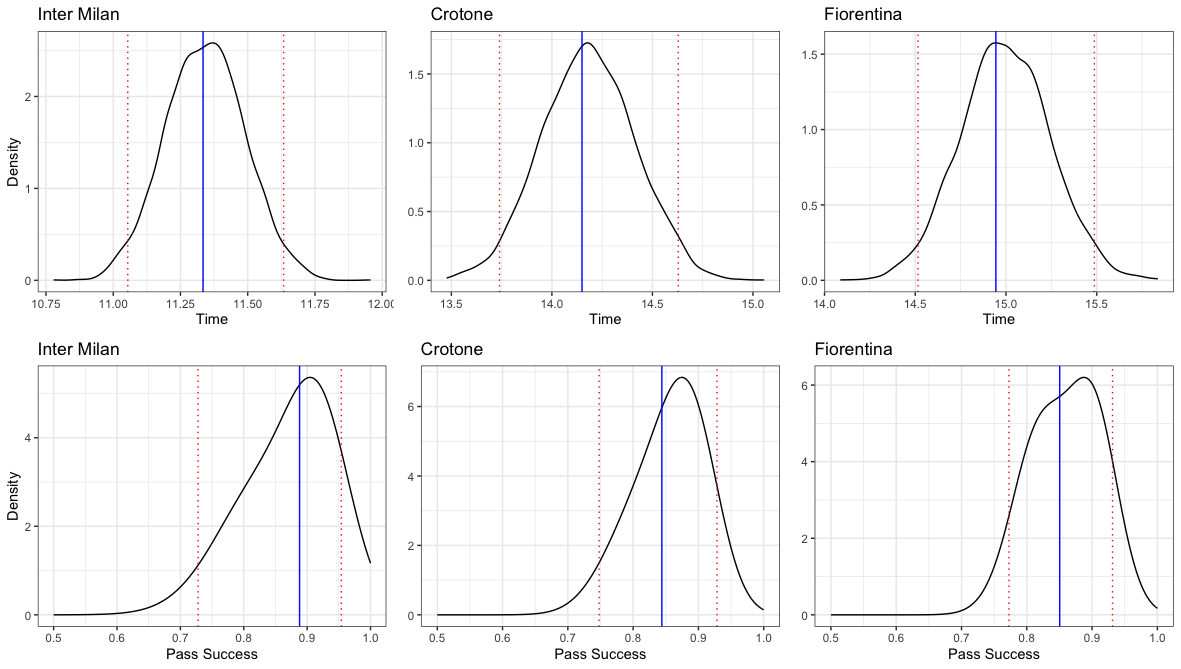
Figure 4: Posterior predictions of the waiting times between passes and the proportions of successful passes by Inter Milan, Crotone, and Fiorentina during the 2020/21 season. The blue-colored solid vertical lines represent the mean of the observed waiting times and the observed proportions of successful passes, while the red-colored dotted vertical lines represent the 2.5% and 97.5% percentiles of the posterior predictions.

Using the posterior draws generated in Section 6, we compare model-based predictions of the waiting times between passes and the proportions of successful passes to the observed waiting times and the observed proportions of successful passes by Inter Milan, Crotone, and Fiorentina during the 2020/21 season. The model-based predictions (i.e., posterior predictions) are shown in Figure 4 in Supplement F and match the observed data.

7 Simulation results

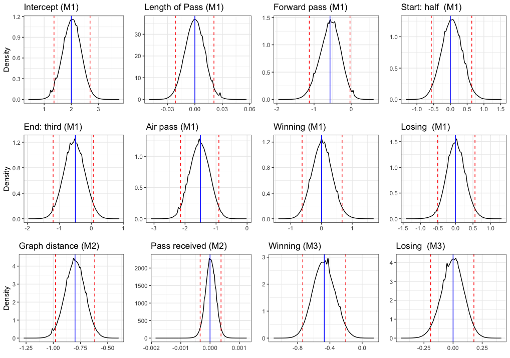
Figure 5: Simulation results: marginal posteriors of selected parameters based on 100 simulated soccer seasons, each with 1,000 passes. The blue-colored solid lines represent the data-generating parameters, while the red-colored dashed lines represent the 2.5% and 97.5% percentiles. M1, M2, and M3 refer to Module M1, M2, and M3 of the stochastic modeling framework specified in Section 6, respectively.

We simulate data from the stochastic modeling framework specified in Section 6. We choose the data-generating parameters of the model so that the simulated data mimic the Inter Milan data in Section 6. We simulate 100 short soccer seasons, each with 1,000 passes. To estimate the model from the 100 simulated soccer seasons, we leverage the Bayesian approach described in Section 5, using the prior described in Section 5. We present in Figure 5 in Supplement G aggregated simulations results based on all 100 simulated soccer seasons. In addition, we present the data-generating parameters along with posterior summaries of the parameters based on one of the 100 simulated soccer seasons in Table 15 in Supplement G. The figure and table demonstrate that the posterior means of the parameters cluster around the data-generating parameters.

8 Discussion

We view the proposed stochastic modeling framework as a first step to modeling soccer matches and other team-based sports as space- and time-indexed network processes and hope that it will stimulate future research. To stimulate future research, we conclude with a short discussion of open questions and directions for future research.

8.1 Model specification

The deluge of high-resolution network data generated by soccer and other team-based sports implies that there are many possible features that may be relevant for predicting ball control, goals, and match outcomes. The specific features used in Section 6 make sense as a starting point, but sound model selection procedures and more data are needed to shed light on which features are useful for predicting ball control, goals, and match outcomes.

In addition, the proposed stochastic modeling framework includes player-specific random effects $\bm{\eta}_{i}\in\mathbb{R}^{3}$, which are correlated within players $i$ but are shared across soccer matches. Since the proposed stochastic modeling framework is already fairly complex, we stick to the player-specific random effects. More advanced latent process models—e.g., multilevel models with position- and team-specific random effects and other more complex latent process models—constitute an interesting direction for future research.

8.2 Data-related challenges

While there is a deluge of high-resolution network data, countless data-related challenges remain. For example, while the stochastic modeling framework can incorporate the spatial distances between soccer players, the existing data is limited to ball-tracking data and does not include player-tracking data. As a result, we know which player is in control of the ball, but we do not know where the players are located on the field. In the application, we therefore used the graph distance based on the formations of soccer teams as an approximation of the spatial distances between players. Note that these limitations are limitations of the data, not the model: The model can leverage both ball-tracking and player-tracking data. Despite these limitations of existing data, we believe that it is important to develop a stochastic modeling framework that can handle data that could and should be collected in the future.

Department of Statistics, University of Missouri-Columbia E-mail: grieshopn@missouri.edu

Department of Economics, University of Missouri-Columbia E-mail: yong.feng@mail.missouri.edu

Department of Biostatistics and Data Science, The University of Texas Health Science Center at Houston E-mail: guanyu.hu@uth.tmc.edu

Department of Statistics, The Pennsylvania State University E-mail: michael.schweinberger@psu.edu

SUPPLEMENT

A CONTINUOUS-TIME STOCHASTIC PROCESS FOR

HIGH-RESOLUTION NETWORK DATA IN SPORTS

Nicholas Grieshop¹, Yong Feng², Guanyu Hu³ and Michael Schweinberger⁴

1 Department of Statistics, University of Missouri-Columbia

2 Department of Economics, University of Missouri-Columbia

3 Department of Biostatistics and Data Science, The University of Texas Health Science Center at Houston

4 Department of Statistics, The Pennsylvania State University

Supplement A: FiguresA
Supplement B: AbbreviationsB
Supplement C: Descriptive statisticsC
Supplement D: Posterior summariesD
Supplement E: Posterior sensitivity checksE
Supplement F: Posterior predictive checksF
Supplement G: Simulation resultsG

Appendix A Figures

Appendix B Abbreviations

Table 1: Abbreviations of player positions.

Player position	Abbreviation
Center Back	CB
Right Center Back	RCB
Left Center Back	LCB
Left Defensive Midfielder	LDMF
Right Defensive Midfielder	RDMF
Right Center Back (3 at the back)	RCB3
Goalkeeper	GK
Defensive Midfielder	DMF
Left Center Midfielder	LCMF
Left Center Back (3 at the back)	LCB3
Right Center Midfielder	RCMF
Left Center Midfielder (3 at the back)	LCMF3
Right Back	RB
Left Back	LB
Attacking Midfielder	AMF
Right Center Midfielder (3 at the back)	RCMF3
Left Attacking Midfielder	LAMF
Left Wing Forward	LWF
Right Wing Forward	RWF
Left Wing	LW
Right Attacking Midfielder	RAMF
Right Wing Back	RWB
Second Striker	SS
Right Wing	RW
Left Wing Back	LWB
Striker	CF
Left Back (5 at the back)	LB5
Right Back (5 at the back)	RB5

Appendix C Descriptive statistics

Table 2: Successful proportion of passes by teams during the 2020/21 season of the Italian premier football league.

	Successful proportion of passes
Team	Total	First half	Second half
Sassuolo	$89.47\%$	$89.97\%$	$88.92\%$
Juventus Turin	$88.95\%$	$89.56\%$	$88.27\%$
Inter Milan	$88.55\%$	$88.69\%$	$88.40\%$
Napoli	$88.10\%$	$88.67\%$	$87.46\%$
Roma	$86.44\%$	$87.17\%$	$85.65\%$
Atalanta	$86.33\%$	$86.33\%$	$86.32\%$
Milan	$86.22\%$	$86.59\%$	$85.82\%$
Lazio	$85.91\%$	$86.36\%$	$85.43\%$
Parma	$85.07\%$	$85.86\%$	$84.27\%$
Udinese	$84.79\%$	$85.57\%$	$84.01\%$
Torino	$84.68\%$	$85.75\%$	$83.53\%$
Fiorentina	$84.50\%$	$85.37\%$	$83.64\%$
Bologna	$84.45\%$	$84.71\%$	$84.17\%$
Spezia	$84.39\%$	$84.84\%$	$83.91\%$
Crotone	$84.28\%$	$84.53\%$	$84.01\%$
Cagliari	$83.50\%$	$84.41\%$	$82.55\%$
Genoa	$83.20\%$	$84.13\%$	$82.27\%$
Benevento	$81.70\%$	$81.52\%$	$81.87\%$
Hellas Verona	$81.39\%$	$82.14\%$	$80.58\%$
Sampdoria	$81.35\%$	$81.97\%$	$80.70\%$

Table 3: Number of passes and successful passes of Juventus Turin during the 2020/21 season, by formation.

Formation	Number of passes	Proportion of successful passes
4-4-2	15832	89.30%
4-4-1-1	1529	88.69%
4-4-1	744	88.04%
3-4-2-1	737	91.18%
4-2-3-1	591	87.14%
3-5-2	455	81.98%
3-4-1-2	261	88.89%
3-5-1-1	147	87.76%
3-4-3	114	81.58%
4-3-1-2	95	84.21%
4-3-2	54	87.04%
4-5-1	39	84.62%
5-3-1	3	66.67%
5-4-1	1	0.00%

Table 4: Number of passes and successful passes of Juventus Turin during the 2020/21 season based on the 4-4-2 formation, by position and player. Danilo refers to the player Danilo Luiz da Silva.

Position	Player	Number of passes	Proportion of successful passes
CF	C. Ronaldo	741	81.38%
	A. Morata	197	76.65%
	P. Dybala	5	80.00%
GK	W. Szczesny	559	95.53%
	G. Buffon	173	91.33%
	C. Pinsoglio	8	87.50%
LB	A. Sandro	769	88.43%
	Danilo	535	91.78%
	G. Frabotta	239	87.45%
	F. Bernardeschi	152	88.16%
	J. Cuadrado	26	92.31%
LCB	G. Chiellini	786	92.75%
	M. de Ligt	518	94.59%
	L. Bonucci	399	90.23%
	Danilo	91	95.60%
	M. Demiral	77	98.70%
	A. Sandro	72	90.28%
LCMF	A. Rabiot	765	92.16%
	R. Bentancur	478	91.84%
	A. Melo	368	95.65%
	W. McKennie	100	87.00%
	N. Fagioli	17	100.00%
	A. Ramsey	9	100.00%
LW	A. Ramsey	400	89.75%
	F. Chiesa	345	79.13%
	F. Bernardeschi	153	81.70%
	W. McKennie	140	85.00%
	D. Kulusevski	51	80.39%
	G. Frabotta	23	78.26%
	F. Correia	8	87.50%
	A. Rabiot	4	100.00%
RB	J. Cuadrado	1010	85.15%
	Danilo	883	88.34%
	M. Demiral	5	80.00%
RCB	M. de Ligt	798	95.49%
	L. Bonucci	627	92.50%
	M. Demiral	328	96.95%
	Danilo	35	97.14%
	R. Drăgușin	2	50.00%
RCMF	R. Bentancur	835	90.30%
	A. Melo	501	94.81%
	A. Rabiot	267	92.51%
	Danilo	145	92.41%
	W. McKennie	129	93.02%
	M. Portanova	5	100.00%
	A. Ramsey	3	100.00%
RW	D. Kulusevski	386	80.05%
	F. Chiesa	243	80.25%
	W. McKennie	164	85.37%
	J. Cuadrado	159	87.42%
	A. Ramsey	82	85.37%
	F. Bernardeschi	19	78.95%
	P. Dybala	4	100.00%
	D. Costa	3	33.33%
	G. Vrioni	2	100.00%
SS	P. Dybala	495	87.88%
	Á. Morata	305	80.33%
	D. Kulusevski	113	80.53%
	C. Ronaldo	73	76.71%
	F. Chiesa	1	0.00%

Table 5: Number of passes and successful passes of Juventus Turin based on the 4-4-2 formation during the 2020/21 season, by player and position.

Player	Position	Number of passes	Proportion of successful passes
C. Ronaldo	CF	908	81.28%
	SS	80	76.25%
	AMF	18	88.89%
D. Kulusevski	RW	386	80.05%
	SS	136	80.88%
	LW	87	79.31%
	AMF	67	83.58%
	RAMF	26	80.77%
	RWF	12	75.00%
	CF	9	66.67%
	RCMF	4	75.00%
	LCMF3	3	33.33%
F. Chiesa	LW	367	79.56%
	RW	294	80.95%
	RWB	44	61.36%
	LAMF	22	72.73%
	LWB	4	50.00%
	RCMF3	4	50.00%
	RAMF	2	50.00%
	SS	1	0.00%
M. de Ligt	RCB	964	95.64%
	LCB	528	94.51%
	RCB3	64	92.19%
	CB	39	92.31%
P. Dybala	SS	512	87.70%
	AMF	81	91.36%
	CF	10	90.00%
	LW	7	85.71%
	RW	4	100.00%
R. Bentancur	RCMF	1042	90.60%
	LCMF	548	91.97%
	DMF	64	85.94%
	RCMF3	20	90.00%
	LCMF3	9	77.78%

Table 6: Number of passes and successful passes of Inter Milan during the 2020/21 season, by formation.

Formation	Number of passes	Proportion of successful passes
3-5-2	13564	88.85%
3-4-1-2	3329	88.80%
5-3-2	1098	85.70%
3-4-3	485	86.19%
4-3-1-2	262	93.51%
5-4-1	172	78.49%
3-4-2-1	110	87.27%
3-4-2	60	90.00%
3-5-1-1	57	89.47%
4-4-1-1	28	85.71%
4-3-2	14	85.71%

Table 7: Number of passes and successful passes of Inter Milan during the 2020/21 season based on the 3-5-2 formation, by position and player.

Position	Player	Number of passes	Proportion of successful passes
CB	S. de Vrij	1371	96.21%
	A. Ranocchia	296	95.95%
CF	R. Lukaku	305	76.72%
	A. Sánchez	174	81.61%
	L. Martínez	136	80.88%
	I. Perišić	5	60.00%
	A. Pinamonti	1	100.00%
DMF	M. Brozović	1518	91.77%
	C. Eriksen	204	88.73%
	N. Barella	60	88.33%
	A. Vidal	28	89.29%
	R. Gagliardini	23	91.30%
GK	S. Handanovič	557	90.84%
	I. Radu	28	100.00%
	D. Padelli	9	100.00%
LCB3	A. Bastoni	1578	92.27%
	M. Škriniar	86	94.19%
	A. Kolarov	43	86.05%
	M. Darmian	25	100.00%
LCMF3	C. Eriksen	419	88.78%
	R. Gagliardini	347	90.78%
	A. Vidal	245	89.39%
	S. Sensi	204	88.73%
	N. Barella	102	90.20%
LWB	I. Perišić	390	77.18%
	A. Young	354	82.20%
	M. Darmian	97	81.44%
	D. D’Ambrosio	5	80.00%
RCB3	M. Škriniar	1526	94.82%
	D. D’Ambrosio	250	93.60%
	S. de Vrij	21	95.24%
RCMF3	N. Barella	1114	84.11%
	A. Vidal	157	84.71%
	M. Vecino	97	86.60%
	S. Sensi	30	86.67%
	C. Eriksen	25	92.00%
	R. Gagliardini	12	83.33%
	R. Nainggolan	2	100.00%
RWB	A. Hakimi	950	82.32%
	M. Darmian	166	83.13%
	A. Young	12	100.00%
	D. D’Ambrosio	5	100.00%
SS	L. Martínez	228	71.49%
	A. Sánchez	165	80.00%
	R. Lukaku	164	71.95%
	A. Pinamonti	26	76.92%

Table 8: Number of passes and successful passes of Inter Milan during the 2020/21 season by famous players in different positions.

Player	Position	Number of passes	Proportion of successful passes
C. Eriksen	LCMF3	507	88.76%
	DMF	212	89.15%
	AMF	141	82.98%
	RCMF3	25	92.00%
	LCMF	8	75.00%
	RCMF	4	100.00%
	SS	4	50.00%
L. Martínez	SS	313	69.33%
	CF	195	78.97%
	LWF	19	73.68%
	LW	2	100.00%
M. Brozović	DMF	1661	91.75%
	RCMF	272	87.50%
	LCMF	108	89.81%
M. Škriniar	RCB3	1950	94.82%
	LCB3	87	93.10%
	RCB	18	94.44%
N. Barella	RCMF3	1245	84.58%
	RCMF	176	91.48%
	LCMF	140	88.57%
	LCMF3	114	90.35%
	DMF	80	88.75%
	AMF	70	88.57%
	RW	8	75.00%
	LWF	4	100.00%
R. Lukaku	CF	462	76.41%
	SS	244	75.00%

Appendix D Posterior summaries

Table 9: Posterior summaries for Fiorentina, Crotone, and Inter Milan (with 3-5-2 formation): M refers to posterior medians and CI refers to 95% posterior credible intervals.

	Fiorentina		Crotone		Inter Milan
	M	CI	M	CI	M	CI
Successful passes $\{S_{i_{m}}=1\}$:
Intercept	2.93	(2.47, 3.39)	3.27	(2.85, 3.68)	3.34	(2.82, 3.86)
Length of pass	0.00	(-0.01, 0.00)	0.00	(-0.01, 0.00)	0.00	(0.00, 0.01)
Forward pass	-0.57	(-0.74, -0.40)	-0.88	(-1.07, -0.70)	-0.84	(-0.99, -0.70)
Start: half	0.17	(-0.02, 0.36)	-0.03	(-0.23, 0.17)	0.29	(0.12, 0.46)
End: third	-0.67	(-0.85, -0.49)	-0.64	(-0.84, -0.45)	-0.79	(-0.96, -0.62)
Air pass	-1.76	(-1.93, -1.59)	-1.90	(-2.07, -1.73)	-1.84	(-1.98, -1.70)
Winning	-0.13	(-0.30, 0.04)	-0.25	(-0.46, -0.04)	-0.13	(-0.26, 0.00)
Losing	-0.01	(-0.17, 0.15)	-0.11	(-0.26, 0.04)	0.02	(-0.16, 0.21)
Passes $\{i_{m}\to j_{m}\}$ given $\{S_{i_{m}}=1\}$:
Graph distance	-0.69	(-0.73, -0.65)	-0.70	(-0.74, -0.65)	-0.98	(-1.02, -0.95)
Pass received	0.00	(-2.3e-3, 2.0e-3)	0.00	(-1.7e-3, 3.2e-4)	0.00	(-1.6e-3, 8.6e-5)
Holding times $h_{m}$:
GK	-3.23	(-3.34, -3.13)	-2.86	(-2.95, -2.77)	-2.98	(-3.06, -2.90)
LCB	-2.62	(-2.68, -2.56)	-2.77	(-2.83, -2.71)	-2.32	(-2.37, -2.27)
CB	-2.62	(-2.70, -2.55)	-2.70	(-2.76, -2.64)	-2.39	(-2.44, -2.34)
RCB	-2.86	(-2.92, -2.79)	-2.44	(-2.51, -2.37)	-2.34	(-2.39, -2.30)
LWB	-2.33	(-2.40, -2.26)	-2.61	(-2.69, -2.53)	-2.27	(-2.34, -2.20)
LCMF	-2.51	(-2.59, -2.43)	-2.50	(-2.57, -2.42)	-2.07	(-2.13, -2.01)
DMF	-2.62	(-2.68, -2.55)	-2.42	(-2.49, -2.36)	-2.13	(-2.18, -2.08)
RCMF	-2.34	(-2.41, -2.26)	-2.62	(-2.70, -2.54)	-2.21	(-2.26, -2.16)
RWB	-2.48	(-2.56, -2.40)	-2.29	(-2.37, -2.20)	-2.01	(-2.07, -1.95)
SS	-2.63	(-2.72, -2.54)	-2.37	(-2.46, -2.28)	-2.11	(-2.19, -2.03)
CF	-2.62	(-2.71, -2.54)	-2.98	(-3.08, -2.88)	-2.30	(-2.38, -2.22)
Winning	-0.42	(-0.47, -0.36)	-0.37	(-0.44, -0.30)	-0.36	(-0.40, -0.33)
Losing	0.05	(0.00, 0.10)	-0.01	(-0.05, 0.04)	-0.08	(-0.13, -0.03)
Random effects:
Correlation	-0.36	(-0.83, 0.12)	-0.25	(-0.75, 0.25)	-0.03	(-0.53, 0.47)
SD: success	0.58	(0.31, 0.86)	0.62	(0.34, 0.89)	0.80	(0.44, 1.17)
SD: pass	0.51	(0.28, 0.74)	0.24	(0.13, 0.36)	0.47	(0.25, 0.69)

Table 10: Posterior summaries for Juventus Turin (with 4-4-2 formation): M refers to posterior medians and CI refers to 95% posterior credible intervals.

Juventus Turin M CI Successful passes $\{S_{i_{m}}=1\}$: Intercept 3.36 (2.90, 3.81) Length of pass 0.00 (-0.01, 0.00) Forward pass -0.61 (-0.75, -0.47) Start: half 0.26 (0.10, 0.42) End: third -0.92 (-1.07, -0.76) Air pass -2.04 (-2.18, -1.89) Winning -0.04 (-0.17, 0.09) Losing 0.04 (-0.13, 0.20) Passes $\{i_{m}\to j_{m}\}$ given $\{S_{i_{m}}=1\}$: Graph distance -0.70 (-0.73, -0.67) Pass received 0.00 (-1.6e-3,  8.6e-05) Holding times $h_{m}$: GK -2.80 (-2.88, -2.72) LB -2.08 (-2.13, -2.03) LCB -2.38 (-2.42, -2.33) RCB -2.37 (-2.41, -2.32) RB -2.09 (-2.14, -2.05) LW -2.06 (-2.12, -2.00) LCMF -2.19 (-2.24, -2.14) RCMF -2.26 (-2.30, -2.21) RW -2.17 (-2.23, -2.11) SS -1.81 (-1.87, -1.74) CF -1.94 (-2.01, -1.87) Winning -0.20 (-0.23, -0.16) Losing -0.15 (-0.19, -0.10) Random effects: Correlation -0.33 (-0.82, 0.15) SD: success 0.69 (0.38, 0.99) SD: pass 0.44 (0.24, 0.64)

Appendix E Posterior sensitivity checks

Table 11: Posterior summaries for Fiorentina, Crotone, and Inter Milan (with 3-5-2 formation) under Prior 1 described in Section 6.1: M refers to posterior medians and CI refers to 95% posterior credible intervals.

	Fiorentina		Crotone		Inter Milan
	M	CI	M	CI	M	CI
Successful passes $\{S_{i_{m}}=1\}$:
Intercept	2.94	(2.56, 3.31)	3.23	(2.82, 3.64)	3.24	(2.74, 3.75)
Length of pass	0.00	(-0.01, 0.00)	0.00	(-0.01, 0.00)	0.00	(-0.01, 0.00)
Forward pass	-0.56	(-0.73, -0.4)	-0.88	(-1.06, -0.71)	-0.84	(-0.99, -0.68)
Start: half	0.15	(-0.04, 0.35)	-0.02	(-0.22, 0.17)	0.29	(0.11, 0.47)
End: third	-0.68	(-0.87, -0.49)	-0.62	(-0.82, -0.43)	-0.79	(-0.97, -0.62)
Air pass	-1.76	(-1.93, -1.59)	-1.90	(-2.07, -1.73)	-1.84	(-1.99, -1.7)
Winning	-0.15	(-0.32, 0.03)	-0.23	(-0.45, -0.02)	-0.12	(-0.25, 0.02)
Losing	-0.01	(-0.19, 0.16)	-0.12	(-0.27, 0.02)	0.01	(-0.17, 0.19)
Passes $\{i_{m}\to j_{m}\}$ given $\{S_{i_{m}}=1\}$:
Graph distance	-0.69	(-0.73, -0.65)	-0.70	(-0.74, -0.65)	-0.99	(-1.02, -0.95)
Pass received	0.00	(-2.09e-3, 1.92e-3)	0.00	(-1.68e-3, 3.13e-4)	0.00	(-1.52e-3, 4.37e-05)
Holding times $h_{m}$:
GK	-3.23	(-3.33, -3.13)	-2.86	(-2.94, -2.77)	-2.98	(-3.06, -2.90)
LCB	-2.62	(-2.68, -2.56)	-2.77	(-2.83, -2.7)	-2.32	(-2.37, -2.27)
CB	-2.62	(-2.69, -2.55)	-2.69	(-2.76, -2.63)	-2.39	(-2.44, -2.34)
RCB	-2.86	(-2.93, -2.79)	-2.44	(-2.5, -2.37)	-2.34	(-2.39, -2.30)
LWB	-2.33	(-2.4, -2.26)	-2.61	(-2.69, -2.53)	-2.27	(-2.34, -2.20)
LCMF	-2.51	(-2.59, -2.43)	-2.50	(-2.57, -2.42)	-2.07	(-2.13, -2.01)
DMF	-2.62	(-2.68, -2.55)	-2.42	(-2.49, -2.36)	-2.13	(-2.18, -2.09)
RCMF	-2.34	(-2.41, -2.26)	-2.62	(-2.7, -2.54)	-2.20	(-2.26, -2.15)
RWB	-2.48	(-2.56, -2.4)	-2.29	(-2.38, -2.19)	-2.01	(-2.07, -1.95)
SS	-2.62	(-2.71, -2.54)	-2.38	(-2.46, -2.29)	-2.12	(-2.21, -2.04)
CF	-2.62	(-2.71, -2.53)	-2.99	(-3.09, -2.89)	-2.30	(-2.38, -2.22)
Winning	-0.41	(-0.47, -0.35)	-0.38	(-0.45, -0.31)	-0.36	(-0.4, -0.33)
Losing	0.06	(0, 0.11)	-0.01	(-0.05, 0.04)	-0.07	(-0.12, -0.02)
Random effects:
Correlation	-0.36	(-0.82, 0.09)	-0.26	(-0.75, 0.23)	-0.05	(-0.56, 0.46)
SD: success	0.58	(0.3, 0.85)	0.62	(0.33, 0.91)	0.82	(0.45, 1.19)
SD: pass	0.50	(0.27, 0.73)	0.24	(0.12, 0.36)	0.46	(0.25, 0.67)

Table 12: Posterior summaries for Juventus Turin (with 4-4-2 formation) under Prior 1 described in Section 6.1: M refers to posterior medians and CI refers to 95% posterior credible intervals.

Juventus Turin M CI Successful passes $\{S_{i_{m}}=1\}$: Intercept 3.38 (2.96, 3.80) Length of pass 0.00 (-0.01, 0.00) Forward pass -0.62 (-0.76, -0.48) Start: half 0.25 (0.09, 0.41) End: third -0.92 (-1.07, -0.76) Air pass -2.04 (-2.18, -1.90) Winning -0.05 (-0.17, 0.08) Losing 0.04 (-0.13, 0.20) Passes $\{i_{m}\to j_{m}\}$ given $\{S_{i_{m}}=1\}$: Graph distance -0.70 (-0.73, -0.67) Pass received 0.00 (-8.12e-4, 6.42e-4) Holding times $h_{m}$: GK -2.80 (-2.88, -2.73) LB -2.08 (-2.13, -2.03) LCB -2.38 (-2.42, -2.33) RCB -2.36 (-2.41, -2.31) RB -2.09 (-2.14, -2.05) LW -2.05 (-2.11, -1.99) LCMF -2.20 (-2.25, -2.15) RCMF -2.26 (-2.3, -2.21) RW -2.16 (-2.23, -2.1) SS -1.80 (-1.86, -1.74) CF -1.93 (-2, -1.86) Winning -0.20 (-0.23, -0.16) Losing -0.15 (-0.19, -0.10) Random effects: Correlation -0.30 (-0.77, 0.17) SD: success 0.68 (0.39, 0.97) SD: pass 0.43 (0.24, 0.62)

Table 13: Posterior summaries for Fiorentina, Crotone, and Inter Milan (with 3-5-2 formation) under Prior 3 described in Section 6.1: M refers to posterior medians and CI refers to 95% posterior credible intervals.

	Fiorentina		Crotone		Inter Milan
	M	CI	M	CI	M	CI
Successful passes $\{S_{i_{m}}=1\}$:
Intercept	2.94	(2.54, 3.34)	3.23	(2.82, 3.65)	3.26	(2.75, 3.76)
Length of pass	0.00	(-0.01, 0)	0.00	(-0.01, 0)	0.00	(0, 0.01)
Forward pass	-0.56	(-0.73, -0.39)	-0.88	(-1.05, -0.7)	-0.84	(-0.99, -0.69)
Start: half	0.17	(-0.02, 0.37)	-0.01	(-0.21, 0.18)	0.30	(0.12, 0.47)
End: third	-0.69	(-0.87, -0.5)	-0.63	(-0.82, -0.44)	-0.79	(-0.97, -0.62)
Air pass	-1.77	(-1.93, -1.6)	-1.90	(-2.06, -1.73)	-1.84	(-1.99, -1.69)
Winning	-0.13	(-0.3, 0.04)	-0.25	(-0.45, -0.05)	-0.12	(-0.25, 0.02)
Losing	-0.02	(-0.18, 0.14)	-0.12	(-0.27, 0.02)	0.02	(-0.16, 0.21)
Passes $\{i_{m}\to j_{m}\}$ given $\{S_{i_{m}}=1\}$:
Graph distance	-0.69	(-0.73, -0.65)	-0.70	(-0.74, -0.66)	-0.99	(-1.02, -0.95)
Pass received	0.00	(-2.0e-3, 2.2e-3)	0.00	(-1.6e-3, 3.8e-4)	0.00	(-1.5e-3, 6.2e-05)
Holding times $h_{m}$:
GK	-3.23	(-3.34, -3.13)	-2.86	(-2.95, -2.77)	-2.98	(-3.06, -2.9)
LCB	-2.62	(-2.69, -2.56)	-2.77	(-2.83, -2.7)	-2.32	(-2.37, -2.27)
CB	-2.62	(-2.69, -2.55)	-2.70	(-2.76, -2.64)	-2.39	(-2.44, -2.34)
RCB	-2.86	(-2.93, -2.79)	-2.44	(-2.5, -2.37)	-2.34	(-2.39, -2.3)
LWB	-2.33	(-2.4, -2.26)	-2.61	(-2.69, -2.53)	-2.28	(-2.34, -2.21)
LCMF	-2.50	(-2.58, -2.42)	-2.50	(-2.57, -2.42)	-2.08	(-2.13, -2.02)
DMF	-2.62	(-2.68, -2.55)	-2.42	(-2.49, -2.36)	-2.13	(-2.18, -2.09)
RCMF	-2.34	(-2.41, -2.26)	-2.62	(-2.7, -2.55)	-2.20	(-2.26, -2.15)
RWB	-2.47	(-2.55, -2.39)	-2.28	(-2.37, -2.19)	-2.01	(-2.07, -1.95)
SS	-2.63	(-2.72, -2.54)	-2.38	(-2.46, -2.29)	-2.12	(-2.2, -2.03)
CF	-2.62	(-2.72, -2.53)	-2.99	(-3.09, -2.89)	-2.30	(-2.38, -2.22)
Winning	-0.42	(-0.47, -0.36)	-0.38	(-0.45, -0.3)	-0.36	(-0.4, -0.33)
Losing	0.05	(0, 0.1)	-0.01	(-0.05, 0.04)	-0.08	(-0.13, -0.02)
Random effects:
Correlation	-0.40	(-0.87, 0.07)	-0.32	(-0.83, 0.18)	-0.08	(-0.61, 0.45)
SD: success	0.58	(0.32, 0.84)	0.60	(0.34, 0.86)	0.78	(0.45, 1.11)
SD: pass	0.50	(0.28, 0.71)	0.23	(0.12, 0.35)	0.44	(0.24, 0.64)

Table 14: Posterior summaries for Juventus Turin (with 4-4-2 formation) using Prior 3 described in Section 6.1: M refers to posterior medians and CI refers to 95% posterior credible intervals.

Juventus Turin M CI Successful passes $\{S_{i_{m}}=1\}$: Intercept 3.35 (2.93, 3.77) Length of pass 0.00 (-0.01, 0) Forward pass -0.62 (-0.75, -0.48) Start: half 0.25 (0.09, 0.41) End: third -0.92 (-1.07, -0.76) Air pass -2.05 (-2.19, -1.91) Winning -0.05 (-0.18, 0.08) Losing 0.04 (-0.13, 0.2) Passes $\{i_{m}\to j_{m}\}$ given $\{S_{i_{m}}=1\}$: Graph distance -0.70 (-0.73, -0.67) Pass received 0.00 (-7.7e-4, 7.1e-4) Holding times $h_{m}$: GK -2.80 (-2.88, -2.73) LB -2.08 (-2.13, -2.03) LCB -2.38 (-2.42, -2.33) RCB -2.36 (-2.41, -2.31) RB -2.09 (-2.14, -2.05) LW -2.06 (-2.12, -2) LCMF -2.20 (-2.25, -2.15) RCMF -2.26 (-2.31, -2.21) RW -2.17 (-2.23, -2.11) SS -1.81 (-1.88, -1.74) CF -1.94 (-2.00, -1.87) Winning -0.20 (-0.23, -0.16) Losing -0.15 (-0.19, -0.1) Random effects: Correlation -0.30 (-0.77, 0.18) SD: success 0.66 (0.37, 0.94) SD: pass 0.42 (0.23, 0.61)

Appendix F Posterior predictive checks

Appendix G Simulation results

Table 15: Simulation results: data-generating parameters and posterior summaries of parameters based on one of the 100 simulated soccer seasons with 1,000 passes. M is the median of the posterior means. CI shows the interval consisting of the 2.5% and 97.5% quantiles of the posterior means.

Simulation Truth M CI Successful passes $\{S_{i_{m}}=1\}$: Intercept 2.00 2.26 (1.78, 2.74) Length of pass 0.00 0.00 (-0.02, 0.01) Forward pass -0.57 -0.72 (-1.1, -0.33) Start: half 0.00 0.00 (-0.43, 0.43) End: third -0.50 -0.43 (-0.88, 0.02) Air pass -1.50 -1.28 (-1.72, -0.85) Winning 0.00 -0.11 (-0.57, 0.34) Losing 0.00 -0.14 (-0.49, 0.22) Passes $\{i_{m}\to j_{m}\}$ given $\{S_{i_{m}}=1\}$: Graph distance -0.80 -0.83 (-0.96, -0.69) Pass received 0.00 0.00 (-3.2e-4, 2.1e-4) Holding times $h_{m}$: GK -2.70 -2.66 (-2.94, -2.37) LCB -2.70 -2.84 (-3.01, -2.66) CB -2.70 -2.66 (-2.85, -2.48) RCB -2.70 -2.60 (-2.8, -2.41) LWB -2.70 -2.71 (-2.98, -2.44) LCMF -2.70 -2.74 (-2.94, -2.55) DMF -2.70 -2.78 (-2.96, -2.59) RCMF -2.70 -2.52 (-2.72, -2.32) RWB -2.70 -2.70 (-2.92, -2.48) SS -2.70 -2.55 (-2.83, -2.28) CF -2.70 -2.70 (-2.97, -2.43) Winning -0.47 -0.58 (-0.77, -0.39) Losing 0.00 0.03 (-0.12, 0.17) Random effects: Correlation 0.00 -0.09 (-0.88, 0.71) SD: success 0.00 0.20 (0.01, 0.38) SD: pass 0.00 0.09 (0, 0.17)

References

- Albert et al. (2017) Albert, J., M. E. Glickman, T. B. Swartz, and R. H. Koning (2017). Handbook of Statistical Methods and Analyses in Sports. Boca Raton, FL: Chapman & Hall/CRC.
- Baio and Blangiardo (2010) Baio, G. and M. Blangiardo (2010). Bayesian hierarchical model for the prediction of football results. Journal of Applied Statistics 37(2), 253–264.
- Beal (2003) Beal, M. J. (2003). Variational Algorithms for Approximate Bayesian Inference. Ph. D. thesis, Gatsby Computational Neuroscience Unit, University College London.
- Blei et al. (2017) Blei, D. M., A. Kucukelbir, and J. D. McAuliffe (2017). Variational inference: A review for statisticians. Journal of the American Statistical Association (Review) 112(518), 859–877.
- Brechot and Flepp (2020) Brechot, M. and R. Flepp (2020). Dealing with randomness in match outcomes: How to rethink performance evaluation in European club football using expected goals. Journal of Sports Economics 21(4), 335–362.
- Butts (2008) Butts, C. T. (2008). A relational event framework for social action. Sociological Methodolgy 38, 155–200.
- Cattelan et al. (2013) Cattelan, M., C. Varin, and D. Firth (2013). Dynamic Bradley–Terry modelling of sports tournaments. Journal of the Royal Statistical Society: Series C (Applied Statistics) 62(1), 135–150.
- Cervone et al. (2014) Cervone, D., A. D’Amour, L. Bornn, and K. Goldsberry (2014). POINTWISE: predicting points and valuing decisions in real time with NBA optical tracking data. In Proceedings of the 8th MIT Sloan Sports Analytics Conference, Boston, MA, USA, Volume 28, pp. 1–9.
- Cervone et al. (2016) Cervone, D., A. D’Amour, L. Bornn, and K. Goldsberry (2016). A multiresolution stochastic process model for predicting basketball possession outcomes. Journal of the American Statistical Association (Applications and Case Studies) 111(514), 585–599.
- Congdon (2019) Congdon, P. D. (2019). Bayesian Hierarchical Models: With Applications Using R. Boca Raton, FL: Chapman & Hall/CRC.
- Dixon and Coles (1997) Dixon, M. J. and S. G. Coles (1997). Modelling association football scores and inefficiencies in the football betting market. Journal of the Royal Statistical Society: Series C (Applied Statistics) 46(2), 265–280.
- Fernandez and Bornn (2018) Fernandez, J. and L. Bornn (2018). Wide open spaces: A statistical technique for measuring space creation in professional soccer. In Sloan Sports Analytics Conference, Volume 2018.
- Franks et al. (2015) Franks, A., A. Miller, L. Bornn, and K. Goldsberry (2015). Characterizing the spatial structure of defensive skill in professional basketball. The Annals of Applied Statistics 9(1), 94–121.
- Hu et al. (2023) Hu, G., H.-C. Yang, Y. Xue, and D. K. Dey (2023). Zero-inflated Poisson model with clustered regression coefficients: Application to heterogeneity learning of field goal attempts of professional basketball players. Canadian Journal of Statistics. To appear.
- Karlis and Ntzoufras (2003) Karlis, D. and I. Ntzoufras (2003). Analysis of sports data by using bivariate Poisson models. Journal of the Royal Statistical Society: Series D (The Statistician) 52(3), 381–393.
- Miller and Bornn (2017) Miller, A. C. and L. Bornn (2017). Possession sketches: Mapping NBA strategies. In Proceedings of the 2017 MIT Sloan Sports Analytics Conference, pp. 1–12.
- Norris (1997) Norris, J. R. (1997). Markov Chains. Cambridge: Cambridge University Press.
- Perry and Wolfe (2013) Perry, P. O. and P. J. Wolfe (2013). Point process modelling for directed interaction networks. Journal of the Royal Statistical Society, Series B (Statistical Methodology) 75, 821–849.
- Sandholtz et al. (2020) Sandholtz, N., J. Mortensen, and L. Bornn (2020). Measuring spatial allocative efficiency in basketball. Journal of Quantitative Analysis in Sports 16(4), 271–289.
- Santos-Fernandez et al. (2022) Santos-Fernandez, E., F. Denti, K. Mengersen, and A. Mira (2022). The role of intrinsic dimension in high-resolution player tracking data—insights in basketball. The Annals of Applied Statistics 16(1), 326–348.
- Sisson et al. (2007) Sisson, S. A., Y. Fan, and M. M. Tanaka (2007). Sequential Monte Carlo without likelihoods. Proceedings of the National Academy of Sciences 104, 1760–1765.
- Stan Development Team (2023) Stan Development Team (2023). RStan: the R interface to Stan. R package version 2.21.8.
- Stroock (2014) Stroock, D. W. (2014). An Introduction to Markov Processes (2 ed.). Heidelberg: Springer.
- Toni et al. (2009) Toni, T., D. Welch, N. Strelkowa, A. Ipsen, and M. P. H. Stumpf (2009). Approximate Bayesian computation scheme for parameter inference and model selection in dynamical systems. Journal of the Royal Society Interface 6, 187–202.
- Wu and Bornn (2018) Wu, S. and L. Bornn (2018). Modeling offensive player movement in professional basketball. The American Statistician 72(1), 72–79.